Embed Size (px)
Citation preview

Deep Neural Networks
Romain HERAULT
Normandie Universite - INSA de Rouen - LITIS
April 29 2015
R. HERAULT (INSA LITIS) Deep Neural Networks April 29 2015 1 / 56
Introduction to supervised learning
Outline
1 Introduction to supervised learning
2 Introduction to Neural Networks
3 Multi-Layer Perceptron - Feed-forward network
4 Deep Neural Networks
5 Extension to structured output
R. HERAULT (INSA LITIS) Deep Neural Networks April 29 2015 2 / 56
Introduction to supervised learning
Supervised learning: Concept
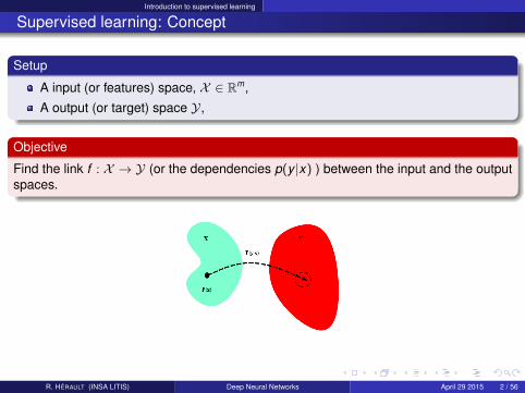
Setup
A input (or features) space, X ∈ Rm,
A output (or target) space Y,
Objective
Find the link f : X → Y (or the dependencies p(y |x) ) between the input and the outputspaces.
R. HERAULT (INSA LITIS) Deep Neural Networks April 29 2015 2 / 56
Introduction to supervised learning
Supervised learning: general framework
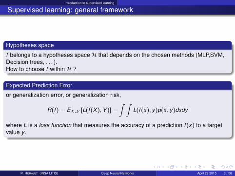
Hypotheses space
f belongs to a hypotheses space H that depends on the chosen methods (MLP,SVM,Decision trees, . . . ).How to choose f within H ?
Expected Prediction Error
or generalization error, or generalization risk,
R(f ) = EX ,Y [L(f (X ),Y )] =
∫ ∫L(f (x), y)p(x , y)dxdy
where L is a loss function that measures the accuracy of a prediction f (x) to a targetvalue y .
R. HERAULT (INSA LITIS) Deep Neural Networks April 29 2015 3 / 56
Introduction to supervised learning
Supervised learning: different tasks, different losses
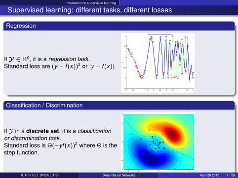
Regression
If Y ∈ Ro, it is a regression task.Standard loss are (y − f (x))2 or |y − f (x)|.
0 0.5 1 1.5 2 2.5 3 3.5 4 4.5 5−1.5
−1
−0.5
0
0.5
1Support Vector Machine Regression
x
y
Classification / Discrimination
If Y in a discrete set, it is a classificationor discrimination task.Standard loss is Θ(−yf (x))2 where Θ is thestep function.
−3 −2 −1 0 1 2 3−3
−2
−1
0
1
2
3
−1
−1
−1
−1
−1
−1
0
0
0
0
0
1
1
1
1
1
R. HERAULT (INSA LITIS) Deep Neural Networks April 29 2015 4 / 56

Introduction to supervised learning
Supervised learning: Experimental setup
Available data
Data consists in a set of n examples (x, y) where x ∈ X and y ∈ Y It is split into:
A training set that will be used to choose f ,i.e. to learn the parameters w of the model
A test set to evaluate the chosen f
(A validation set to choose the hyper-parameters of f )
Because of the human cost of labelling data, one can found a separate unlabelled set,i.e. examples with only the feature x (see semi-supervised learning)
Evaluation: Empirical risk
RS(f ) =1
card(S)
n∑(x,y)∈S
L(f (x), y)
where S is the train set during learning, the test set during final evaluation.
R. HERAULT (INSA LITIS) Deep Neural Networks April 29 2015 5 / 56
Introduction to supervised learning
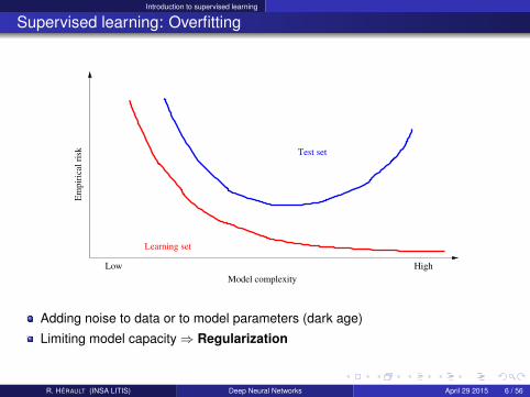
Supervised learning: Overfitting
Em
piri
cal r
isk Test set
Learning set
Low HighModel complexity
Adding noise to data or to model parameters (dark age)
Limiting model capacity⇒ Regularization
R. HERAULT (INSA LITIS) Deep Neural Networks April 29 2015 6 / 56
Introduction to supervised learning
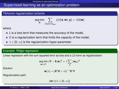
Supervised learning as an optimization problem
Tikhonov regularization scheme
arg minw
∑(x,y)∈Strain
L(f (x; w), y) + λΩ(w)
where
L is a loss term that measures the accuracy of the model,
Ω is a regularization term that limits the capacity of the model,
λ ∈ [0,∞[ is the regularization hyper-parameter.
Example: Ridge regression
Linear regression with the sum squared error as loss and a L2-norm as regularization:
arg minw∈Rd
||Y− X.w||2 + λ∑
d
||wd ||2
Solutionw(λ) = (XᵀX + λI)−1XᵀY
Regularization path:
w(λ)|λ ∈ [0,∞[
R. HERAULT (INSA LITIS) Deep Neural Networks April 29 2015 7 / 56
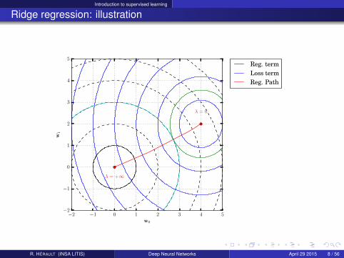
Introduction to supervised learning
Ridge regression: illustration
−2 −1 0 1 2 3 4 5w0
−2
−1
0
1
2
3
4
5w
1
λ = 0
λ = +∞
Reg. termLoss termReg. Path
R. HERAULT (INSA LITIS) Deep Neural Networks April 29 2015 8 / 56
Introduction to supervised learning
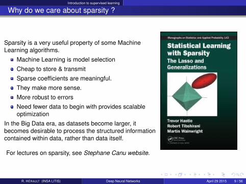
Why do we care about sparsity ?
Sparsity is a very useful property of some MachineLearning algorithms.
Machine Learning is model selection
Cheap to store & transmit
Sparse coefficients are meaningful.
They make more sense.
More robust to errors
Need fewer data to begin with provides scalableoptimization
In the Big Data era, as datasets become larger, itbecomes desirable to process the structured informationcontained within data, rather than data itself.
For lectures on sparsity, see Stephane Canu website.
R. HERAULT (INSA LITIS) Deep Neural Networks April 29 2015 9 / 56
Introduction to supervised learning
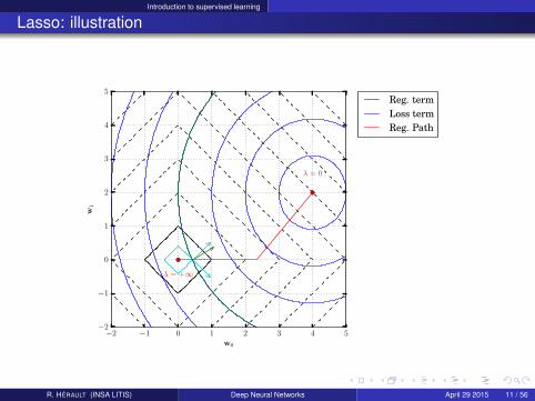
Introducing sparsity
Lasso
Linear regression with the sum squared error as loss and a L1-norm as regularization:
arg minw∈Rd
||Y− X.w||2 + λ∑
d
|wd |
which is equivalent to
arg minw+∈Rd ,w−∈Rd
||Y− X.(w+ −w−)||2 + λ∑
d (w+ + w−)
s.t .
w+i ≥ 0 ∀i ∈ [1..d ]
w−i ≥ 0 ∀i ∈ [1..d ]
Why is it sparse ?
R. HERAULT (INSA LITIS) Deep Neural Networks April 29 2015 10 / 56
Introduction to supervised learning
Lasso: illustration
−2 −1 0 1 2 3 4 5w0
−2
−1
0
1
2
3
4
5w
1
λ = 0
λ = +∞
Reg. termLoss termReg. Path
R. HERAULT (INSA LITIS) Deep Neural Networks April 29 2015 11 / 56
Introduction to Neural Networks
Outline
1 Introduction to supervised learning
2 Introduction to Neural Networks
3 Multi-Layer Perceptron - Feed-forward network
4 Deep Neural Networks
5 Extension to structured output
R. HERAULT (INSA LITIS) Deep Neural Networks April 29 2015 12 / 56

Introduction to Neural Networks
History . . .
1940 : Turing machine
1943 : Formal neuron (Mc Culloch & Pitts)
1948 : Automate networks (Von Neuman)
1949 : First learning rules (Hebb)
1957 : Perceptron (Rosenblatt)
1960 : Adaline (Widrow & Hoff)1969 : Perceptrons (Minsky & Papert)
Limitation of the perceptronNeed for more complex architectures, but then how to learn?
1974 : Gradient back-propagation (Werbos)no success !?!?
R. HERAULT (INSA LITIS) Deep Neural Networks April 29 2015 12 / 56
Introduction to Neural Networks
History . . .
1986 : Gradient back-propagation bis (Rumelhart & McClelland, Lecun)New neural networks architecturesNew Applications :
Character recognitionSpeech recognition and synthesisVision (image processing)
1990-2010 : Information societyNew fields
Web crawlersInformation extractionMultimedia (indexation,. . . ).Data-mining
Needs to combine many models and build adequate features1992-1995 : Kernel methods
Support Vector Machine (Boser, Guyon and Vapnik)2005 : Deep networks
Deep Belief Machine, DBM (Hinton and Salakhutdinov, 2006)Deep Neural Network, DNN
R. HERAULT (INSA LITIS) Deep Neural Networks April 29 2015 13 / 56
Introduction to Neural Networks
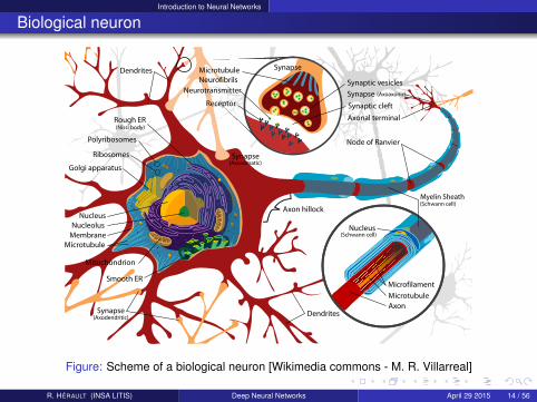
Biological neuron
Figure: Scheme of a biological neuron [Wikimedia commons - M. R. Villarreal]
R. HERAULT (INSA LITIS) Deep Neural Networks April 29 2015 14 / 56
Introduction to Neural Networks
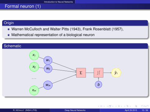
Formal neuron (1)
Origin
Warren McCulloch and Walter Pitts (1943), Frank Rosenblatt (1957),
Mathematical representation of a biological neuron
Schematic
x1
x2
xm
. . .
Σ cd
b
y1
w1
w2
wm
R. HERAULT (INSA LITIS) Deep Neural Networks April 29 2015 15 / 56

Introduction to Neural Networks
Formal neuron (2)
Formulation
y = f (〈w, x〉+ b) (1)
where
x, input vector,
y , output estimation,
w, weights linked to each input (model parameter),
b, bias (model parameter),
f , activation function.
EvaluationTypical losses are
Classification
L(y , y) = − (y .log(y) + (1− y).log(1− y))
Regression
L(y , y) = ||y − y ||2
R. HERAULT (INSA LITIS) Deep Neural Networks April 29 2015 16 / 56

Introduction to Neural Networks
Formal neuron (3)
Activation functions are typically step function, sigmoid function ([0 1]) or hyperbolictangent ([−1 1]).
x
f (x)f (x) = sigm(x)
1
1
Figure: Sigmoid
x
f (x)f (x) = tanh(x)
1
1
Figure: Hyperbolic tangent
If loss and activation function are differentiable, parameters w and b can be learned bygradient descent.
R. HERAULT (INSA LITIS) Deep Neural Networks April 29 2015 17 / 56
Introduction to Neural Networks
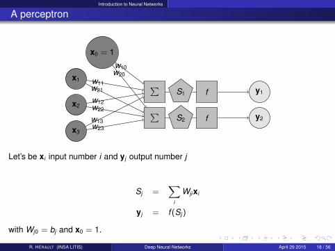
A perceptron
x3
x2
x1
x0 = 1
∑∑
S2
S1
f
f
y2
y1
w23w13
w22w12
w21w11
w20w10
Let’s be xi input number i and yj output number j
Sj =∑
i
Wjixi
yj = f (Sj )
with Wj0 = bj and x0 = 1.
R. HERAULT (INSA LITIS) Deep Neural Networks April 29 2015 18 / 56
Introduction to Neural Networks
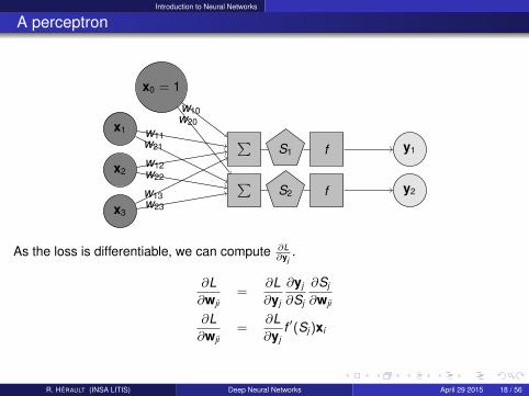
A perceptron
x3
x2
x1
x0 = 1
∑∑
S2
S1
f
f
y2
y1
w23w13
w22w12
w21w11
w20w10
As the loss is differentiable, we can compute ∂L∂yj
.
∂L∂wji
=∂L∂yj
∂yj
∂Sj
∂Sj
∂wji
∂L∂wji
=∂L∂yj
f ′(Sj )xi
R. HERAULT (INSA LITIS) Deep Neural Networks April 29 2015 18 / 56
Introduction to Neural Networks
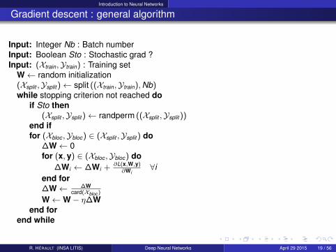
Gradient descent : general algorithm
Input: Integer Nb : Batch numberInput: Boolean Sto : Stochastic grad ?Input: (Xtrain,Ytrain) : Training set
W← random initialization(Xsplit ,Ysplit )← split ((Xtrain,Ytrain),Nb)while stopping criterion not reached do
if Sto then(Xsplit ,Ysplit )← randperm ((Xsplit ,Ysplit ))
end iffor (Xbloc ,Ybloc) ∈ (Xsplit ,Ysplit ) do
∆W← 0for (x, y) ∈ (Xbloc ,Ybloc) do
∆Wi ← ∆Wi + ∂L(x,W,y)∂Wi
∀iend for∆W← ∆W
card(Xbloc )
W← W− η∆Wend for
end while
R. HERAULT (INSA LITIS) Deep Neural Networks April 29 2015 19 / 56
Introduction to Neural Networks
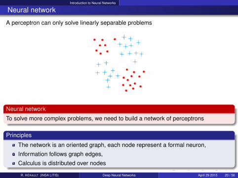
Neural network
A perceptron can only solve linearly separable problems
Neural network
To solve more complex problems, we need to build a network of perceptrons
Principles
The network is an oriented graph, each node represent a formal neuron,
Information follows graph edges,
Calculus is distributed over nodes
R. HERAULT (INSA LITIS) Deep Neural Networks April 29 2015 20 / 56
Introduction to Neural Networks
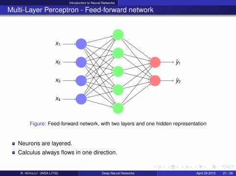
Multi-Layer Perceptron - Feed-forward network
x1
x2
x3
x4
y1
y2
Figure: Feed-forward network, with two layers and one hidden representation
Neurons are layered.
Calculus always flows in one direction.
R. HERAULT (INSA LITIS) Deep Neural Networks April 29 2015 21 / 56
Introduction to Neural Networks
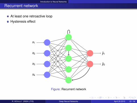
Recurrent network
At least one retroactive loop
Hysteresis effect
x1
x2
x3
x4
y1
y2
Figure: Recurrent network
R. HERAULT (INSA LITIS) Deep Neural Networks April 29 2015 22 / 56
Introduction to Neural Networks
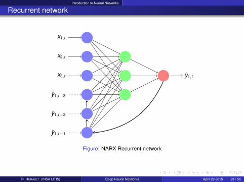
Recurrent network
x1,t
x2,t
x3,t
y1,t−3
y1,t−2
y1,t−1
y1,t
Figure: NARX Recurrent network
R. HERAULT (INSA LITIS) Deep Neural Networks April 29 2015 23 / 56

Multi-Layer Perceptron - Feed-forward network
Outline
1 Introduction to supervised learning
2 Introduction to Neural Networks
3 Multi-Layer Perceptron - Feed-forward network
4 Deep Neural Networks
5 Extension to structured output
R. HERAULT (INSA LITIS) Deep Neural Networks April 29 2015 24 / 56
Multi-Layer Perceptron - Feed-forward network
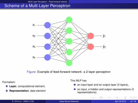
Scheme of a Multi Layer Perceptron
x1
x2
x3
x4
y1
y2
Figure: Example of feed-forward network: a 2-layer perceptron
Formalism:
Layer, computational element,
Representation, data element
This MLP has
an input layer and an output layer (2 layers),
an input, a hidden and output representations (3representations).
R. HERAULT (INSA LITIS) Deep Neural Networks April 29 2015 24 / 56

Multi-Layer Perceptron - Feed-forward network
Estimation of y: Forward path
I(l)3
I(l)2
I(l)1
I(l)0 = 1
∑∑
S(l)2
S(l)1
f (l)
f (l)
O(l)2
O(l)1
w23w13
w22w12
w21w11
w20w10
If we look at layer (l), let’s be I(l)i input number i and O(l)
j output number j ,
S(l)j =
∑i
W (l)ji I(l)
i
O(l)j = f (l)(S(l)
j ) = I(l+1)
Starts with I(0) = x and finishes with O(last) = y
R. HERAULT (INSA LITIS) Deep Neural Networks April 29 2015 25 / 56
Multi-Layer Perceptron - Feed-forward network
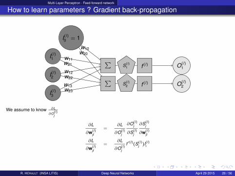
How to learn parameters ? Gradient back-propagation
I(l)3
I(l)2
I(l)1
I(l)0 = 1
∑∑
S(l)2
S(l)1
f (l)
f (l)
O(l)2
O(l)1
w23w13
w22w12
w21w11
w20w10
We assume to know ∂L
∂O(l)j
∂L
∂w(l)ji
=∂L
∂O(l)j
∂O(l)j
∂S(l)j
∂S(l)j
∂w(l)ji
∂L
∂w(l)ji
=∂L
∂O(l)j
f ′(l)(S(l)j )I(l)
i
R. HERAULT (INSA LITIS) Deep Neural Networks April 29 2015 26 / 56
Multi-Layer Perceptron - Feed-forward network
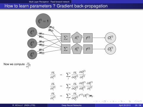
How to learn parameters ? Gradient back-propagation
I(l)3
I(l)2
I(l)1
I(l)0 = 1
∑∑
S(l)2
S(l)1
f (l)
f (l)
O(l)2
O(l)1
w23w13
w22w12
w21w11
w20w10
Now we compute ∂L
∂I(l)i
∂L
∂I(l)i
=∑
j
∂L
∂O(l)j
∂O(l)j
∂I(l)i
∂L
∂I(l)i
=∑
j
∂L
∂O(l)j
∂O(l)j
∂S(l)j
∂S(l)j
∂I(l)i
∂L
∂I(l)i
=∑
j
∂L
∂O(l)j
f ′(l)(S(l)j )wji
R. HERAULT (INSA LITIS) Deep Neural Networks April 29 2015 26 / 56

Multi-Layer Perceptron - Feed-forward network
How to learn parameters ? Gradient back-propagation
I(l)3
I(l)2
I(l)1
I(l)0 = 1
∑∑
S(l)2
S(l)1
f (l)
f (l)
O(l)2
O(l)1
w23w13
w22w12
w21w11
w20w10
Start ∂L
∂O(last)j
= ∂L∂yj
Backward recurrence∂L
∂w(l)ji
=∂L
∂O(l)j
f ′(l)(S(l)j )I(l)
i
∂L
∂I(l)i
=∑
j
∂L
∂O(l)j
f ′(l)(S(l)j )wji
∂L
∂O(l−1)j
=∂L
∂I(l)i
R. HERAULT (INSA LITIS) Deep Neural Networks April 29 2015 26 / 56
Deep Neural Networks
Outline
1 Introduction to supervised learning
2 Introduction to Neural Networks
3 Multi-Layer Perceptron - Feed-forward network
4 Deep Neural Networks
5 Extension to structured output
R. HERAULT (INSA LITIS) Deep Neural Networks April 29 2015 27 / 56

Deep Neural Networks
Deep architecture
x1
x2
x3
x4
x5
y1
Why ?
Some problems needs exponential number of neurons on the hiddenrepresentation,
Build / extract features inside the NN in order not to rely on handmade extraction(human prior).
R. HERAULT (INSA LITIS) Deep Neural Networks April 29 2015 27 / 56
Deep Neural Networks
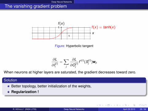
The vanishing gradient problem
x
f (x)f (x) = tanh(x)
1
1
Figure: Hyperbolic tangent
∂L
∂I(l)i
=∑
j
∂L
∂O(l)j
f ′(l)(S(l)j )wji
When neurons at higher layers are saturated, the gradient decreases toward zero.
Solution
Better topology, better initialization of the weights,
Regularization !
R. HERAULT (INSA LITIS) Deep Neural Networks April 29 2015 28 / 56
Deep Neural Networks
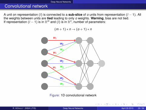
Convolutional network
A unit on representation (l) is connected to a sub-slice of o units from representation (l − 1). Allthe weights between units are tied leading to only o weights. Warning, bias are not tied.If representation (l − 1) is in Rm and (l) is in Rn, number of parameters:
(m + 1) ∗ n→ (o + 1) ∗ n
w1
w2
w3w1
w2
w3w1
w2
w3
Figure: 1D convolutional network
R. HERAULT (INSA LITIS) Deep Neural Networks April 29 2015 29 / 56
Deep Neural Networks
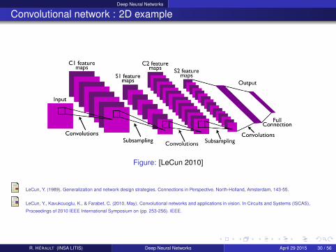
Convolutional network : 2D example
Figure: [LeCun 2010]
LeCun, Y. (1989). Generalization and network design strategies. Connections in Perspective. North-Holland, Amsterdam, 143-55.
LeCun, Y., Kavukcuoglu, K., & Farabet, C. (2010, May). Convolutional networks and applications in vision. In Circuits and Systems (ISCAS),
Proceedings of 2010 IEEE International Symposium on (pp. 253-256). IEEE.
R. HERAULT (INSA LITIS) Deep Neural Networks April 29 2015 30 / 56
Deep Neural Networks
Better initialization through unsupervised learning
The learning is split into two steps:
Pre-training
A unsupervised pre-training of the input layers with auto-encoders. Intuition: learningthe manifold where the input data resides.Can take into account an unlabelled dataset.
Finetuning
A finetuning of the whole network with supervised back-propagation.
Hinton, G. E., Osindero, S. and Teh, Y. (2006) A fast learning algorithm for deep belief nets. Neural Computation, 18, pp 1527-1554
Hinton, G. E. and Salakhutdinov, R. R. (2006) Reducing the dimensionality of data with neural networks. Science, Vol. 313. no. 5786, pp. 504 - 507,
28 July 2006.
R. HERAULT (INSA LITIS) Deep Neural Networks April 29 2015 31 / 56
Deep Neural Networks
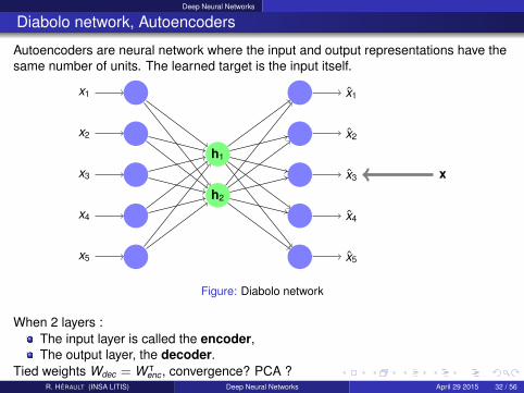
Diabolo network, Autoencoders
Autoencoders are neural network where the input and output representations have thesame number of units. The learned target is the input itself.
h1
h2
x1
x2
x3
x4
x5
x1
x2
x3
x4
x5
x
Figure: Diabolo network
When 2 layers :The input layer is called the encoder,The output layer, the decoder.
Tied weights Wdec = W ᵀenc , convergence? PCA ?
R. HERAULT (INSA LITIS) Deep Neural Networks April 29 2015 32 / 56

Deep Neural Networks
Diabolo network, Autoencoders
Autoencoders are neural network where the input and output representations have thesame number of units. The learned target is the input itself.
h1
h2
x1
x2
x3
x4
x5
x1
x2
x3
x4
x5
x
Figure: Diabolo network
Undercomplete, size(h) < size(x)
Overcomplete, size(x) < size(h).
R. HERAULT (INSA LITIS) Deep Neural Networks April 29 2015 32 / 56
Deep Neural Networks
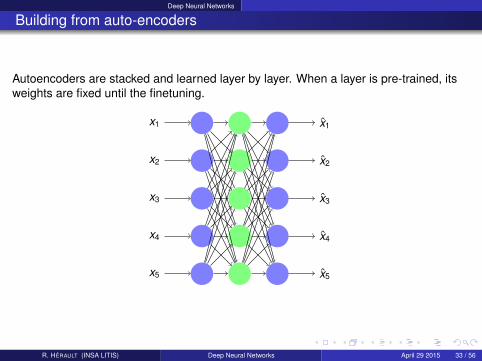
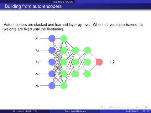
Building from auto-encoders
Autoencoders are stacked and learned layer by layer. When a layer is pre-trained, itsweights are fixed until the finetuning.
x1
x2
x3
x4
x5
x1
x2
x3
x4
x5
R. HERAULT (INSA LITIS) Deep Neural Networks April 29 2015 33 / 56
Deep Neural Networks
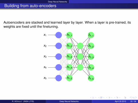
Building from auto-encoders
Autoencoders are stacked and learned layer by layer. When a layer is pre-trained, itsweights are fixed until the finetuning.
h1,1
h1,2
h1,3
h1,4
h1,5
h1,1
h1,2
h1,3
h1,4
h1,5
x1
x2
x3
x4
x5
R. HERAULT (INSA LITIS) Deep Neural Networks April 29 2015 33 / 56
Deep Neural Networks
Building from auto-encoders
Autoencoders are stacked and learned layer by layer. When a layer is pre-trained, itsweights are fixed until the finetuning.
h2,1
h2,2
h2,3
h2,1
h2,2
h2,3
x1
x2
x3
x4
x5
R. HERAULT (INSA LITIS) Deep Neural Networks April 29 2015 33 / 56
Deep Neural Networks
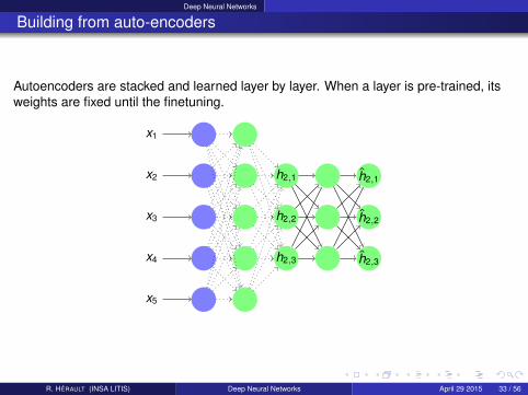
Building from auto-encoders
Autoencoders are stacked and learned layer by layer. When a layer is pre-trained, itsweights are fixed until the finetuning.
x1
x2
x3
x4
x5
y1
R. HERAULT (INSA LITIS) Deep Neural Networks April 29 2015 33 / 56
Deep Neural Networks
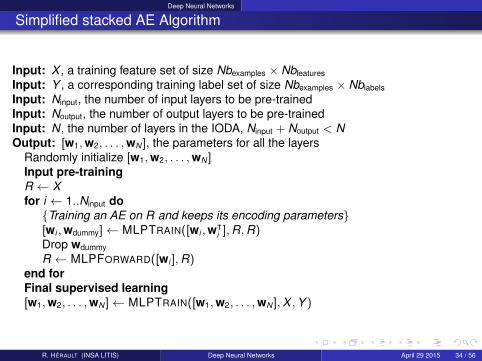
Simplified stacked AE Algorithm
Input: X , a training feature set of size Nbexamples × Nbfeatures
Input: Y , a corresponding training label set of size Nbexamples × Nblabels
Input: Ninput, the number of input layers to be pre-trainedInput: Noutput, the number of output layers to be pre-trainedInput: N, the number of layers in the IODA, Ninput + Noutput < NOutput: [w1,w2, . . . ,wN ], the parameters for all the layers
Randomly initialize [w1,w2, . . . ,wN ]Input pre-trainingR ← Xfor i ← 1..Ninput doTraining an AE on R and keeps its encoding parameters[wi ,wdummy]← MLPTRAIN([wi ,wᵀ
i ],R,R)Drop wdummy
R ← MLPFORWARD([wi ],R)end forFinal supervised learning[w1,w2, . . . ,wN ]← MLPTRAIN([w1,w2, . . . ,wN ],X ,Y )
R. HERAULT (INSA LITIS) Deep Neural Networks April 29 2015 34 / 56

Deep Neural Networks
Improve optimization by adding noise 1/3
Denoising (undercomplete) auto-encoders
The auto-encoder is learned from x, a disturbed x; the target is still x.
x1
x2
x3
x4
x5
h1
h2
x1
x2
x3
x4
x5
x1
x2
x3
x4
x5
Dis
turb
ance
x
R. HERAULT (INSA LITIS) Deep Neural Networks April 29 2015 35 / 56

Deep Neural Networks
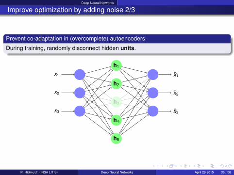
Improve optimization by adding noise 2/3
Prevent co-adaptation in (overcomplete) autoencoders
During training, randomly disconnect hidden units.
h1
h2
h4
h5
x1
x2
x3
x1
x2
x3
h3
R. HERAULT (INSA LITIS) Deep Neural Networks April 29 2015 36 / 56
Deep Neural Networks
Improve optimization by adding noise 2/3
Prevent co-adaptation in (overcomplete) autoencoders
During training, randomly disconnect hidden units.
h1
h2
h4
h5
x1
x2
x3
x1
x2
x3
h3
R. HERAULT (INSA LITIS) Deep Neural Networks April 29 2015 36 / 56
Deep Neural Networks
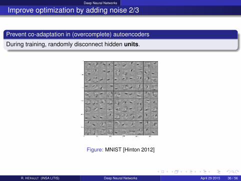
Improve optimization by adding noise 2/3
Prevent co-adaptation in (overcomplete) autoencoders
During training, randomly disconnect hidden units.
Figure: MNIST [Hinton 2012]
R. HERAULT (INSA LITIS) Deep Neural Networks April 29 2015 36 / 56
Deep Neural Networks
Improve optimization by adding noise 3/3
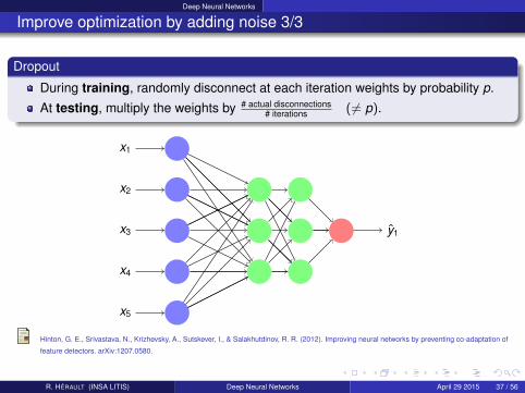
Dropout
During training, randomly disconnect at each iteration weights by probability p.
At testing, multiply the weights by # actual disconnections# iterations ( 6= p).
x1
x2
x3
x4
x5
y1
Hinton, G. E., Srivastava, N., Krizhevsky, A., Sutskever, I., & Salakhutdinov, R. R. (2012). Improving neural networks by preventing co-adaptation of
feature detectors. arXiv:1207.0580.
R. HERAULT (INSA LITIS) Deep Neural Networks April 29 2015 37 / 56
Deep Neural Networks
Improve optimization by adding noise 3/3
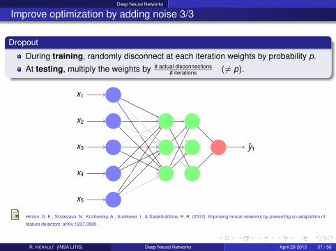
Dropout
During training, randomly disconnect at each iteration weights by probability p.
At testing, multiply the weights by # actual disconnections# iterations ( 6= p).
x1
x2
x3
x4
x5
y1
Hinton, G. E., Srivastava, N., Krizhevsky, A., Sutskever, I., & Salakhutdinov, R. R. (2012). Improving neural networks by preventing co-adaptation of
feature detectors. arXiv:1207.0580.
R. HERAULT (INSA LITIS) Deep Neural Networks April 29 2015 37 / 56
Deep Neural Networks
Improve optimization by adding noise 3/3
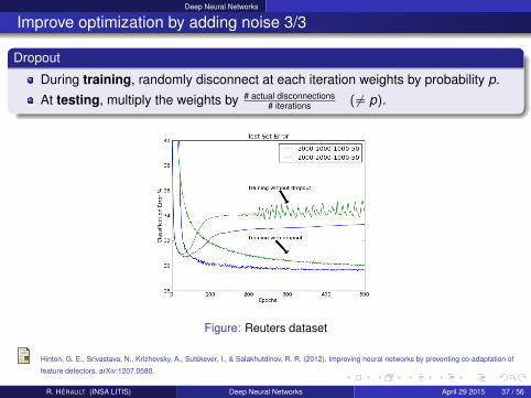
Dropout
During training, randomly disconnect at each iteration weights by probability p.
At testing, multiply the weights by # actual disconnections# iterations ( 6= p).
Figure: Reuters dataset
Hinton, G. E., Srivastava, N., Krizhevsky, A., Sutskever, I., & Salakhutdinov, R. R. (2012). Improving neural networks by preventing co-adaptation of
feature detectors. arXiv:1207.0580.
R. HERAULT (INSA LITIS) Deep Neural Networks April 29 2015 37 / 56
Deep Neural Networks
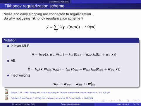
Tikhonov regularization scheme
Noise and early stopping are connected to regularization.So why not using Tikhonov regularization scheme ?
J =∑
i
L(yi , f (xi ; w)) + λ.Ω(w)
Notation
2-layer MLP
y = fMLP(x; win,wout ) = fout (bout + wout .fin(bin + win.x))
AE
x = fAE (x; wenc ,wdec) = fdec (bdec + wdec .fenc(benc + wenc .x))
Tied weights
win ↔ wenc , wdec ↔ wᵀenc
Bishop, C. M. (1995). Training with noise is equivalent to Tikhonov regularization. Neural computation, 7(1), 108-116
Collobert, R. and Bengio, S. (2004). Links between perceptrons, MLPs and SVMs. In ICML’2004
R. HERAULT (INSA LITIS) Deep Neural Networks April 29 2015 38 / 56
Deep Neural Networks
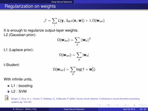
Regularization on weights
J =∑
i
L(yi , fMLP(xi ; w)) + λ.Ω(wout )
It is enough to regularize output-layer weights.L2 (Gaussian prior):
Ω(wout ) =∑
d
||wd ||2
L1 (Laplace prior):Ω(wout ) =
∑d
|wd |
t-Student:Ω(wout ) =
∑d
log(1 + w2d )
With infinite units,
L1 : boosting
L2 : SVM
Bengio, Y., Roux, N. L., Vincent, P., Delalleau, O., & Marcotte, P. (2005). Convex neural networks. In Advances in neural information processing
systems (pp. 123-130)
R. HERAULT (INSA LITIS) Deep Neural Networks April 29 2015 39 / 56
Deep Neural Networks
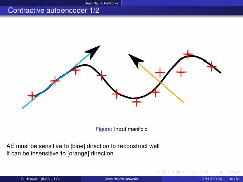
Contractive autoencoder 1/2
Figure: Input manifold
AE must be sensitive to [blue] direction to reconstruct wellIt can be insensitive to [orange] direction.
R. HERAULT (INSA LITIS) Deep Neural Networks April 29 2015 40 / 56
Deep Neural Networks
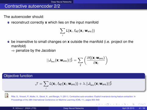
Contractive autoencoder 2/2
The autoencoder should:
reconstruct correctly x which lies on the input manifold∑i
L(xi , fAE (xi ; wenc))
be insensitive to small changes on x outside the manifold (i.e. project on themanifold)⇒ penalize by the Jacobian
||Jfenc (x; wenc)||2F =∑
ij
(∂fj (x; wenc)
∂xi
)
Objective function
J =∑
i
L(xi , fAE (xi ; wenc)) + λ.||Jfenc (x; wenc)||2F
Rifai, S., Vincent, P., Muller, X., Glorot, X., and Bengio, Y. (2011). Contractive auto-encoders: Explicit invariance during feature extraction. In
Proceedings of the 28th International Conference on Machine Learning (ICML-11), pages 833–840
R. HERAULT (INSA LITIS) Deep Neural Networks April 29 2015 41 / 56
Deep Neural Networks
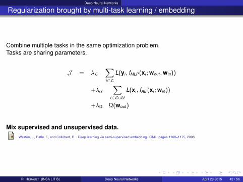
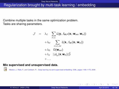
Regularization brought by multi-task learning / embedding
Combine multiple tasks in the same optimization problem.Tasks are sharing parameters.
J = λL∑i∈L
L(yi , fMLP(xi ; wout ,win))
+λU∑
i∈L∪U
L(xi , fAE (xi ; win))
+λΩ Ω(wout )
Mix supervised and unsupervised data.Weston, J., Ratle, F., and Collobert, R. . Deep learning via semi-supervised embedding. ICML, pages 1168–1175, 2008
R. HERAULT (INSA LITIS) Deep Neural Networks April 29 2015 42 / 56
Deep Neural Networks
Regularization brought by multi-task learning / embedding
Combine multiple tasks in the same optimization problem.Tasks are sharing parameters.
J = λL∑i∈L
L(yi , fMLP(xi ; wout ,win))
+λU∑
i∈L∪U
L(xi , fAE (xi ; win))
+λΩ Ω(wout )
+λJ ||Jfin (x; win)||2F+ . . .
Mix supervised and unsupervised data.Weston, J., Ratle, F., and Collobert, R. . Deep learning via semi-supervised embedding. ICML, pages 1168–1175, 2008
R. HERAULT (INSA LITIS) Deep Neural Networks April 29 2015 42 / 56
Extension to structured output
Outline
1 Introduction to supervised learning
2 Introduction to Neural Networks
3 Multi-Layer Perceptron - Feed-forward network
4 Deep Neural Networks
5 Extension to structured output
R. HERAULT (INSA LITIS) Deep Neural Networks April 29 2015 43 / 56
Extension to structured output
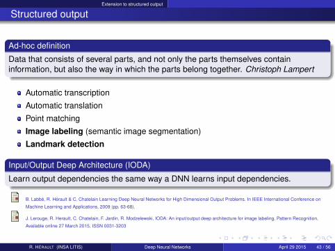
Structured output
Ad-hoc definition
Data that consists of several parts, and not only the parts themselves containinformation, but also the way in which the parts belong together. Christoph Lampert
Automatic transcription
Automatic translation
Point matching
Image labeling (semantic image segmentation)
Landmark detection
Input/Output Deep Architecture (IODA)
Learn output dependencies the same way a DNN learns input dependencies.
B. Labbe, R. Herault & C. Chatelain Learning Deep Neural Networks for High Dimensional Output Problems. In IEEE International Conference on
Machine Learning and Applications, 2009 (pp. 63-68).
J. Lerouge, R. Herault, C. Chatelain, F. Jardin, R. Modzelewski, IODA: An input/output deep architecture for image labeling, Pattern Recognition,
Available online 27 March 2015, ISSN 0031-3203
R. HERAULT (INSA LITIS) Deep Neural Networks April 29 2015 43 / 56
Extension to structured output
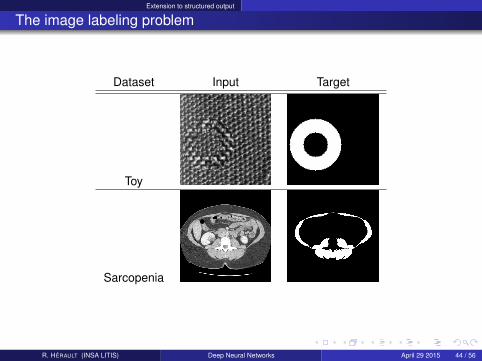
The image labeling problem
Dataset Input Target
Toy
Sarcopenia
R. HERAULT (INSA LITIS) Deep Neural Networks April 29 2015 44 / 56
Extension to structured output
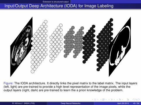
Input/Output Deep Architecture (IODA) for Image Labeling
Figure: The IODA architecture. It directly links the pixel matrix to the label matrix. The input layers(left, light) are pre-trained to provide a high level representation of the image pixels, while theoutput layers (right, dark) are pre-trained to learn the a priori knowledge of the problem.
R. HERAULT (INSA LITIS) Deep Neural Networks April 29 2015 45 / 56
Extension to structured output
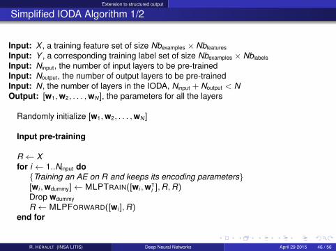
Simplified IODA Algorithm 1/2
Input: X , a training feature set of size Nbexamples × Nbfeatures
Input: Y , a corresponding training label set of size Nbexamples × Nblabels
Input: Ninput, the number of input layers to be pre-trainedInput: Noutput, the number of output layers to be pre-trainedInput: N, the number of layers in the IODA, Ninput + Noutput < NOutput: [w1,w2, . . . ,wN ], the parameters for all the layers
Randomly initialize [w1,w2, . . . ,wN ]
Input pre-training
R ← Xfor i ← 1..Ninput doTraining an AE on R and keeps its encoding parameters[wi ,wdummy]← MLPTRAIN([wi ,wᵀ
i ],R,R)Drop wdummy
R ← MLPFORWARD([wi ],R)end for
R. HERAULT (INSA LITIS) Deep Neural Networks April 29 2015 46 / 56
Extension to structured output
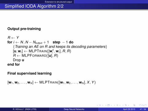
Simplified IODA Algorithm 2/2
Output pre-training
R ← Yfor i ← N..N − Noutput + 1 step − 1 doTraining an AE on R and keeps its decoding parameters[u,wi ]← MLPTRAIN([wᵀ
i ,wi ],R,R)R ← MLPFORWARD([u],R)Drop u
end for
Final supervised learning
[w1,w2, . . . ,wN ]← MLPTRAIN([w1,w2, . . . ,wN ],X ,Y )
R. HERAULT (INSA LITIS) Deep Neural Networks April 29 2015 47 / 56
Extension to structured output
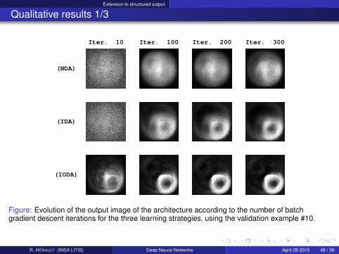
Qualitative results 1/3
(NDA)
(IDA)
(IODA)
Iter. 10 Iter. 100 Iter. 200 Iter. 300
Figure: Evolution of the output image of the architecture according to the number of batchgradient descent iterations for the three learning strategies, using the validation example #10.
R. HERAULT (INSA LITIS) Deep Neural Networks April 29 2015 48 / 56
Extension to structured output
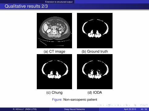
Qualitative results 2/3
(a) CT image (b) Ground truth
(c) Chung (d) IODA
Figure: Non-sarcopenic patient
R. HERAULT (INSA LITIS) Deep Neural Networks April 29 2015 49 / 56

Extension to structured output
Qualitative results 3/3
(a) CT image (b) Ground truth
(c) Chung (d) IODA
Figure: Sarcopenic patient
R. HERAULT (INSA LITIS) Deep Neural Networks April 29 2015 50 / 56
Extension to structured output
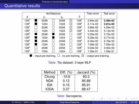
Quantitative results
Architecture Train error Test errorX r1 r2 Y
1282 2048 2048 1282 2.64e-02 3.48e-021282 1024 1024 1282 3.11e-02 3.91e-021282 2048 2048 1282 3.86e-02 4.59e-021282 1024 1024 1282 4.44e-02 5.13e-021282 2048 2048 1282 5.20e-02 5.75e-021282 1024 1024 1282 6.29e-02 6.77e-021282 2048 2048 1282 6.30e-02 6.79e-021282 1024 1024 1282 7.09e-02 7.55e-021282 2048 2048 1282 9.03e-02 9.40e-021282 1024 1024 1282 1.03e-01 1.06e-01
: input pre-training, : no pre-training, : output pre-training.
Table: Toy dataset: 3-layer MLP
Method Diff. (%) Jaccard (%)Chung -10.6 60.3NDA 0.12 85.88IDA 0.15 85.91
IODA 3.37 88.47
Table: Sarcopenia.
R. HERAULT (INSA LITIS) Deep Neural Networks April 29 2015 51 / 56
Extension to structured output
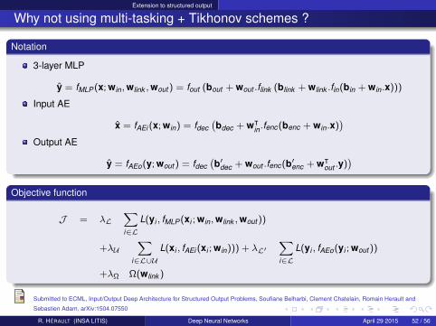
Why not using multi-tasking + Tikhonov schemes ?
Notation
3-layer MLP
y = fMLP(x; win,wlink ,wout ) = fout (bout + wout .flink (blink + wlink .fin(bin + win.x)))
Input AE
x = fAEi (x; win) = fdec(bdec + wᵀ
in.fenc(benc + win.x))
Output AE
y = fAEo(y; wout ) = fdec(b′dec + wout .fenc(b′enc + wᵀ
out .y))
Objective function
J = λL∑i∈L
L(yi , fMLP(xi ; win,wlink ,wout ))
+λU∑
i∈L∪UL(xi , fAEi (xi ; win))) + λL′
∑i∈L
L(yi , fAEo(yi ; wout ))
+λΩ Ω(wlink )
Submitted to ECML, Input/Output Deep Architecture for Structured Output Problems, Soufiane Belharbi, Clement Chatelain, Romain Herault and
Sebastien Adam, arXiv:1504.07550
R. HERAULT (INSA LITIS) Deep Neural Networks April 29 2015 52 / 56
Extension to structured output
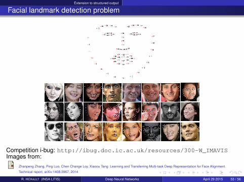
Facial landmark detection problem
Competition i-bug: http://ibug.doc.ic.ac.uk/resources/300-W_IMAVISImages from:
Zhanpeng Zhang, Ping Luo, Chen Change Loy, Xiaoou Tang. Learning and Transferring Multi-task Deep Representation for Face Alignment.
Technical report, arXiv:1408.3967, 2014
R. HERAULT (INSA LITIS) Deep Neural Networks April 29 2015 53 / 56
Extension to structured output
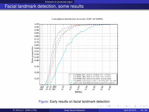
Facial landmark detection, some results
Figure: Early results on facial landmark detection
R. HERAULT (INSA LITIS) Deep Neural Networks April 29 2015 54 / 56

Extension to structured output
Questions ?
?R. HERAULT (INSA LITIS) Deep Neural Networks April 29 2015 55 / 56
Extension to structured output
References
Y. Bengio, A. Courville, P. Vincent, ”Representation Learning: A Review and New Perspectives,” IEEE Transactions on Pattern Analysis and Machine
Intelligence, vol. 35, no. 8, pp. 1798-1828, Aug., 2013 (arXiv:1206.5538)
Bengio, Y. (2012). Practical recommendations for gradient-based training of deep architectures. In Neural Networks: Tricks of the Trade (pp.
437-478). Springer Berlin Heidelberg.
Hinton, G. E., Srivastava, N., Krizhevsky, A., Sutskever, I., & Salakhutdinov, R. R. (2012). Improving neural networks by preventing co-adaptation of
feature detectors. (arXiv:1207.0580).
LeCun, Y., Kavukcuoglu, K., & Farabet, C. (2010, May). Convolutional networks and applications in vision. In Circuits and Systems (ISCAS),
Proceedings of 2010 IEEE International Symposium on (pp. 253-256). IEEE.
J. Lerouge, R. Herault, C. Chatelain, F. Jardin, R. Modzelewski, IODA: An input/output deep architecture for image labeling, Pattern Recognition,
Available online 27 March 2015, ISSN 0031-3203, http://dx.doi.org/10.1016/j.patcog.2015.03.017.
Hugo Larochelle lectures:http://info.usherbrooke.ca/hlarochelle/cours/ift725_A2013/contenu.html
R. HERAULT (INSA LITIS) Deep Neural Networks April 29 2015 56 / 56