Embed Size (px)
Citation preview
Deep Neural Network Approximation TheoryPhilipp Grohs, Dmytro Perekrestenko, Dennis Elbrachter, and Helmut Bolcskei
Abstract
Deep neural networks have become state-of-the-art technology for a wide range of practical machine learning
tasks such as image classification, handwritten digit recognition, speech recognition, or game intelligence. This
paper develops the fundamental limits of learning in deep neural networks by characterizing what is possible if no
constraints on the learning algorithm and the amount of training data are imposed. Concretely, we consider information-
theoretically optimal approximation through deep neural networks with the guiding theme being a relation between
the complexity of the function (class) to be approximated and the complexity of the approximating network in terms
of connectivity and memory requirements for storing the network topology and the associated quantized weights.
The theory we develop educes remarkable universality properties of deep networks. Specifically, deep networks are
optimal approximants for vastly different function classes such as affine systems and Gabor systems. Affine systems are
generated by the affine group (scalings and translations) whereas Gabor systems are generated by the Weyl-Heisenberg
group (time-shifts and modulations). This universality is afforded by a concurrent invariance property of deep networks
to time-shifts, scalings, and frequency-shifts. In addition, deep networks provide exponential approximation accuracy—
i.e., the approximation error decays exponentially in the number of non-zero weights in the network—of vastly different
functions such as the squaring operation, multiplication, polynomials, sinusoidal functions, general smooth functions,
and even one-dimensional oscillatory textures and fractal functions such as the Weierstrass function, both of which
do not have any known methods achieving exponential approximation accuracy. In summary, deep neural networks
provide information-theoretically optimal approximation of a very wide range of functions and function classes used in
mathematical signal processing. We also show that in the approximation of sufficiently smooth functions finite-width
deep networks require strictly smaller connectivity than finite-depth wide networks.
I. INTRODUCTION
Triggered by the availability of vast amounts of training data and drastic improvements in computing power,
deep neural networks have become state-of-the-art technology for a wide range of practical machine learning tasks
P. Grohs is with the Department of Mathematics and the Research Platform DataScience@UniVienna, University of Vienna, Austria (e-mail:
D. Elbrachter is with the Department of Mathematics, University of Vienna, Austria (e-mail: [email protected]).
D. Perekrestenko is with the Department of Information Technology and Electrical Engineering, ETH Zurich, Switzerland (e-mail:
H. Bolcskei is with the Department of Information Technology and Electrical Engineering and the Department of Mathematics, ETH Zurich,
Switzerland (e-mail: [email protected]).
D. Perekrestenko and H. Bolcskei were supported in part by a gift from Huawei’s Future Network Theory Lab. D. Elbrachter was supported
by the Austrian Science Fund via the project P 30148.
arX
iv:1
901.
0222
0v1
[cs
.LG
] 8
Jan
201
9
such as image classification [1], handwritten digit recognition [2], speech recognition [3], or game intelligence [4].
For an in-depth overview, we refer to the survey paper [5] and the recent book [6].
A neural network effectively implements a mapping approximating a function which is learned based on a given
set of input-output value pairs, typically through the backpropagation algorithm [7]. Characterizing the fundamental
limits of approximation through neural networks shows what is possible if no constraints on the learning algorithm
and on the amount of training data are imposed [8].
It is well known that single-hidden-layer neural networks can approximate continuous functions on bounded
domains arbitrarily well, provided that the activation function satisfies certain (mild) conditions and the number of
nodes is allowed to grow arbitrarily large [9], [10], [11]. In practice one is, however, often interested in approximating
functions from a given function class C determined by the application at hand. It is therefore natural to ask how the
complexity of a neural network approximating every function in C to within a prescribed accuracy depends on the
complexity of C (and on the desired approximation accuracy). The recently developed Kolmogorov rate-distortion-
theoretic approach [12] formalizes this question by relating the complexity of C—in terms of the number of bits
needed to describe any element in C to within prescribed accuracy—to network complexity in terms of connectivity
and memory requirements for storing the network topology and the associated quantized weights.
The purpose of this paper is to provide a comprehensive, principled, and self-contained introduction to Kol-
mogorov rate-distortion optimal approximation through deep neural networks. The idea is to equip the reader with
a working knowledge of the mathematical tools underlying the theory at a level that is sufficiently deep to enable
further own research in the field. Part of this paper is based on [12], but extends the theory therein to the rectified
linear unit (ReLU) activation function and to networks with depth scaling in the approximation error.
The theory we develop educes remarkable universality properties of finite-width deep networks. Specifically,
deep networks are optimal approximants for vastly different function classes such as affine systems [12] and
Gabor systems and local cosine bases [13], [14]. Affine systems are generated by the affine group (scalings and
translations) whereas Gabor systems and local cosine bases are generated by the Weyl-Heisenberg group (time-
shifts and modulations). This universality is afforded by a concurrent invariance property of deep networks to time-
shifts, scalings, and frequency-shifts. In addition, deep networks provide exponential approximation accuracy—i.e.,
the approximation error decays exponentially in the number of parameters employed in the approximant, namely
the number of non-zero weights in the network—of vastly different functions such as the squaring operation,
multiplication, polynomials, sinusoidal functions, general smooth functions, and even one-dimensional oscillatory
textures [15] and fractal functions such as the Weierstrass function, both of which do not have any known methods
achieving exponential approximation accuracy. In summary, deep neural networks provide optimal approximation
of a very wide range of functions and function classes used in mathematical signal processing.
While we consider networks based on the ReLU activation function throughout, the parts of our theory not
involving sinusoidal functions, i.e., everything apart from Sections IV and VIII, can be shown to also apply to
2
strongly sigmoidal activation functions of order k ≥ 2 as defined in [12]. The key to this extension is to note that
the result on the neural network approximation of the multiplication function according to Theorem III.2 holds for
strongly sigmoidal activation functions of order k ≥ 2 as well. The rest of the theory then follows mutatis mutandis.
We do not provide the details here for the sake of conciseness.
Notation. For the function f(x) : Rd → R, we define ‖f‖L∞(Ω) := infC ≥ 0 : |f(x)| ≤ C, for all x ∈ Ω.
Lp(Rd) and Lp(Rd,C) denote the space of real-valued, respectively complex-valued, Lp-functions. For a vector
b ∈ Rd, we let ‖b‖∞ := maxi=1,...,d |bi|, similarly we write ‖A‖∞ := maxi,j |Ai,j | for the matrix A ∈ Rm×n.
We denote the identity matrix of size n × n by In. Throughout, log stands for the logarithm to base 2. For a set
X ∈ Rd, we write |X| for its Lebesgue measure.
II. SETUP AND BASIC RELU CALCULUS
There is a plethora of neural network architectures and activation functions in the literature. Here, we restrict
ourselves to the ReLU activation function and consider the following general network architecture.
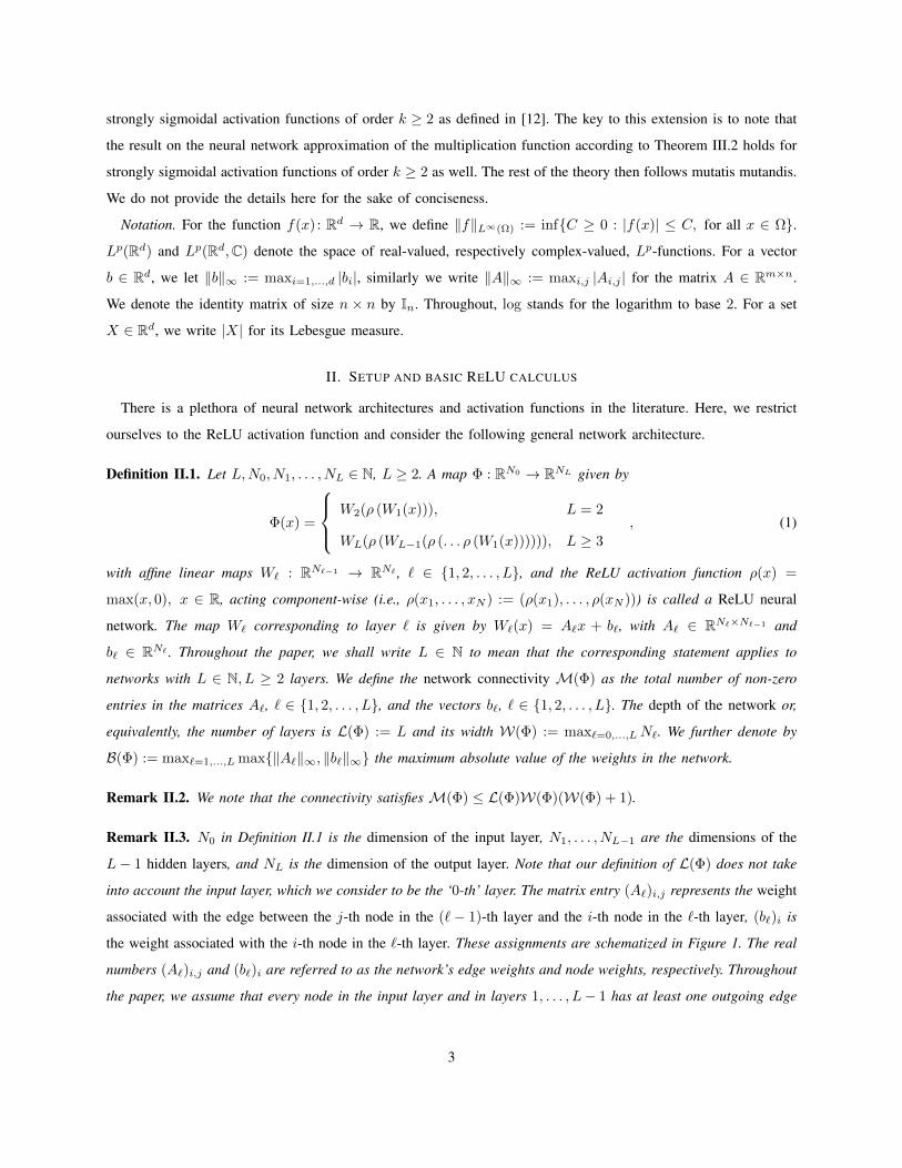
Definition II.1. Let L,N0, N1, . . . , NL ∈ N, L ≥ 2. A map Φ : RN0 → RNL given by
Φ(x) =
W2(ρ (W1(x))), L = 2
WL(ρ (WL−1(ρ (. . . ρ (W1(x)))))), L ≥ 3
, (1)
with affine linear maps W` : RN`−1 → RN` , ` ∈ 1, 2, . . . , L, and the ReLU activation function ρ(x) =
max(x, 0), x ∈ R, acting component-wise (i.e., ρ(x1, . . . , xN ) := (ρ(x1), . . . , ρ(xN ))) is called a ReLU neural
network. The map W` corresponding to layer ` is given by W`(x) = A`x + b`, with A` ∈ RN`×N`−1 and
b` ∈ RN` . Throughout the paper, we shall write L ∈ N to mean that the corresponding statement applies to
networks with L ∈ N, L ≥ 2 layers. We define the network connectivity M(Φ) as the total number of non-zero
entries in the matrices A`, ` ∈ 1, 2, . . . , L, and the vectors b`, ` ∈ 1, 2, . . . , L. The depth of the network or,
equivalently, the number of layers is L(Φ) := L and its width W(Φ) := max`=0,...,LN`. We further denote by
B(Φ) := max`=1,...,L max‖A`‖∞, ‖b`‖∞ the maximum absolute value of the weights in the network.
Remark II.2. We note that the connectivity satisfies M(Φ) ≤ L(Φ)W(Φ)(W(Φ) + 1).
Remark II.3. N0 in Definition II.1 is the dimension of the input layer, N1, . . . , NL−1 are the dimensions of the
L− 1 hidden layers, and NL is the dimension of the output layer. Note that our definition of L(Φ) does not take
into account the input layer, which we consider to be the ‘0-th’ layer. The matrix entry (A`)i,j represents the weight
associated with the edge between the j-th node in the (`− 1)-th layer and the i-th node in the `-th layer, (b`)i is
the weight associated with the i-th node in the `-th layer. These assignments are schematized in Figure 1. The real
numbers (A`)i,j and (b`)i are referred to as the network’s edge weights and node weights, respectively. Throughout
the paper, we assume that every node in the input layer and in layers 1, . . . , L− 1 has at least one outgoing edge
3
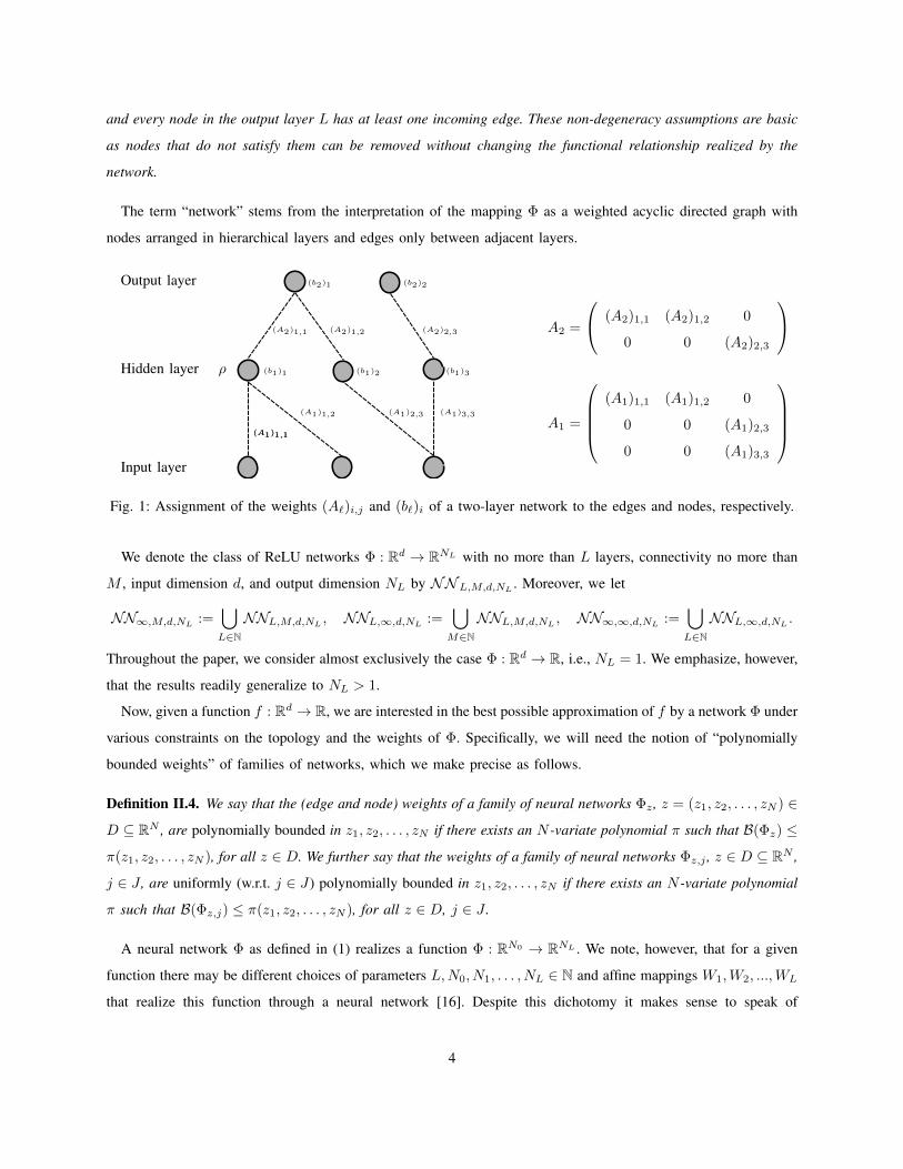
and every node in the output layer L has at least one incoming edge. These non-degeneracy assumptions are basic
as nodes that do not satisfy them can be removed without changing the functional relationship realized by the
network.
The term “network” stems from the interpretation of the mapping Φ as a weighted acyclic directed graph with
nodes arranged in hierarchical layers and edges only between adjacent layers.
(b2)1 (b2)2
(b1)1 (b1)2 (b1)3
(A2)1,1 (A2)1,2 (A2)2,3
(A1)1,1
(A1)3,3(A1)2,3(A1)1,2
(A1)1,1
A2 =
(A2)1,1 (A2)1,2 0
0 0 (A2)2,3
A1 =
(A1)1,1 (A1)1,2 0
0 0 (A1)2,3
0 0 (A1)3,3
Output layer
Hidden layer ρ
Input layer
Fig. 1: Assignment of the weights (A`)i,j and (b`)i of a two-layer network to the edges and nodes, respectively.
We denote the class of ReLU networks Φ : Rd → RNL with no more than L layers, connectivity no more than
M , input dimension d, and output dimension NL by NNL,M,d,NL . Moreover, we let
NN∞,M,d,NL :=⋃L∈NNNL,M,d,NL , NNL,∞,d,NL :=
⋃M∈N
NNL,M,d,NL , NN∞,∞,d,NL :=⋃L∈NNNL,∞,d,NL .
Throughout the paper, we consider almost exclusively the case Φ : Rd → R, i.e., NL = 1. We emphasize, however,
that the results readily generalize to NL > 1.
Now, given a function f : Rd → R, we are interested in the best possible approximation of f by a network Φ under
various constraints on the topology and the weights of Φ. Specifically, we will need the notion of “polynomially
bounded weights” of families of networks, which we make precise as follows.
Definition II.4. We say that the (edge and node) weights of a family of neural networks Φz , z = (z1, z2, . . . , zN ) ∈
D ⊆ RN , are polynomially bounded in z1, z2, . . . , zN if there exists an N -variate polynomial π such that B(Φz) ≤
π(z1, z2, . . . , zN ), for all z ∈ D. We further say that the weights of a family of neural networks Φz,j , z ∈ D ⊆ RN ,
j ∈ J , are uniformly (w.r.t. j ∈ J) polynomially bounded in z1, z2, . . . , zN if there exists an N -variate polynomial
π such that B(Φz,j) ≤ π(z1, z2, . . . , zN ), for all z ∈ D, j ∈ J .
A neural network Φ as defined in (1) realizes a function Φ : RN0 → RNL . We note, however, that for a given
function there may be different choices of parameters L,N0, N1, . . . , NL ∈ N and affine mappings W1,W2, ...,WL
that realize this function through a neural network [16]. Despite this dichotomy it makes sense to speak of
4
compositions and linear combinations of neural networks. To this end, we first record a technical lemma on the
composition of neural networks as defined in [17].
Lemma II.5. Let L1, L2,M1,M2, d1, d2, NL1 , NL2 ∈ N, Φ1 ∈ NNL1,M1,d1,NL1, and Φ2 ∈ NNL2,M2,d2,NL2
with NL1= d2. Then, there exists a network Ψ ∈ NNL1+L2,2M1+2M2,d1,NL2
with W(Ψ) ≤ max2NL1,W(Φ1),
W(Φ2) and B(Ψ) = maxB(Φ1),B(Φ2), satisfying Ψ(x) = Φ2(Φ1(x)), for all x ∈ Rd1 .
Proof. The proof is based on the identity x = ρ(x)− ρ(−x). First, note that by Definition II.1, we can write
Φ1(x) = W 1L1
( ρ ( . . . W 11 (x))) and Φ2(x) = W 2
L2( ρ ( . . . W 2
1 (x))).
Next, define the affine map given by W (x) = W 21
((INL1
−INL1
)x
), for x ∈ R2NL1 , and note that thanks to
W 21 (Φ1(x)) = W
ρ W 1
L1
−W 1L1
( ρ ( . . .W 11 (x)))
,
the map
Ψ(x) = W 2L2
ρ. . .W 2
2
ρW
ρ W 1
L1
−W 1L1
( ρ ( . . .W 11 (x)))
satisfies Ψ(x) = Φ2(Φ1(x)), for all x ∈ Rd1 , with L(Ψ) = L1 + L2, M(Ψ) ≤ 2M1 + 2M2, W(Ψ1) ≤
max2NL1 ,W(Φ1),W(Φ2), and B(Ψ) ≤ maxB(Φ1),B(Φ2).
Before we can formalize the concept of a linear combination of neural networks, we need a result that shows
how to augment network depth while retaining the network’s input-output relation.
Lemma II.6. Let L,M,K, d ∈ N, Φ1 ∈ NNL,M,d,1, and K > L. Then, there exists a corresponding network Φ2 ∈
NNK,M+W(Φ1)+2(K−L)+1,d,1 such that Φ2(x) = Φ1(x), for all x ∈ Rd. Moreover, W(Φ2) = max2,W(Φ1)
and the weights of Φ2 consist of the weights of Φ1 and ±1’s.
Proof. The proof is based on the identity x = ρ(x) − ρ(−x). First, note that by (1) we can write Φ1(x) =
WL( ρ ( . . .W1(x))). For K = L+ 1, Φ2 is given by
Φ2(x) =(
1 −1)ρ
WL
−WL
( ρ ( . . .W1(x)))
∈ NNL+1,M+W(Φ1)+3,d,1. (2)
For K > L+ 1, consider the network
Φ′1(x) =
ρ(Φ1(x))
ρ(−Φ1(x))
=
1 0
0 1
ρ
WL
−WL
( ρ ( . . .W1(x)))
∈ NNL+1,M+W(Φ1)+3,d,2, (3)
which satisfies W(Φ′1) = max2,W(Φ1). Next, we note that for every network of the form Ψ(x) = I2 ρ ( . . . ),
the network
Ψ′(x) := I2 ρ (Ψ(x)), (4)
5
satisfies Ψ′(x) = Ψ(x), for all x ∈ Rd, L(Ψ′) = L(Ψ) + 1, and M(Ψ′) =M(Ψ) + 2. Moreover, the weights of
Ψ′ consist of the weights of Ψ and 1. Noting that Φ′1 in (3) is of the form I2 ρ ( . . . ) and iteratively applying the
operation in (4) K−L− 2 times to Φ′1, we obtain a network Φ′′1 ∈ NNK−1,M+W(Φ1)+2(K−L)−1,d,2. The proof is
concluded by noting that Φ2 = (1 − 1)ρ (Φ′′1) ∈ NNK,M+W(Φ1)+2(K−L)+1,d,1 satisfies Φ2(x) = Φ1(x), for all
x ∈ Rd.
The next result formalizes the concept of a linear combination of neural networks.
Lemma II.7. Let N,Li,Mi, di ∈ N, ai ∈ R, Φi ∈ NNLi,Mi,di,1, i = 1, 2, . . . , N , d =∑Ni=1 di. Then,
there exist networks Φ1 ∈ NNL,M,d,N and Φ2 ∈ NNL,M+N,d,1 with L = maxi Li, W(Φ1) = W(Φ2) ≤∑Ni=1 max2,W(Φi), and M =
∑Ni=1(Mi +W(Φi) + 2(L− Li) + 1) satisfying
Φ1(x) = (a1Φ1(x1) a2Φ2(x2) . . . aNΦN (xN ))T and
Φ2(x) =
N∑i=1
aiΦi(xi),
for all x = (xT1 , xT2 , . . . , x
TN )T ∈ Rd with xi ∈ Rdi , i = 1, 2, . . . , N . Moreover, the weights of Φ1,Φ2 consist of
the weights of the Φi, i = 1, 2, . . . , N , a1, a2, ..., aN, and ±1’s.
Proof. Apply Lemma II.6 to the networks Φi to get corresponding networks Φi of depth L and set Φ1(x) :=(a1Φ1(x1), a2Φ2(x2), . . . , aN ΦN (xN )
)>, Φ2(x) := (1, 1, . . . , 1)Φ1(x).
III. APPROXIMATION OF MULTIPLICATION, POLYNOMIALS, AND SMOOTH FUNCTIONS
We start with the approximation of the multiplication operation by deep ReLU networks and then proceed to the
approximation of polynomials. Specifically, we shall be interested in networks that approximate to within error ε,
are of finite width, and have depth scaling poly-logarithmically in ε−1 (i.e., as a polynomial in log(ε−1)) and (edge
and node) weights that do not grow faster than polynomially in the size of the domain over which approximation
takes place. It will be shown in Section V that this combination of requirements leads to exponential approximation
accuracy for individual signals, i.e., the approximation error decays exponentially in the number of nodes in the
network, and to rate-distortion optimal approximation of signal classes.
The proof ideas for the results in this section are partly inspired by [18] and the “sawtooth” construction of [19].
In contrast to [18], we consider networks without “skip connections” and of finite and explicitly specified width.
Proposition III.1. There exists a constant C > 0 such that for all ε ∈ (0, 1/2), there is a network Φε ∈ NN∞,∞,1,1satisfying L(Φε) ≤ C log(ε−1), W(Φε) = 4, B(Φε) ≤ 4, Φε(0) = 0, and
‖Φε(x)− x2‖L∞([0,1]) ≤ ε. (5)
Proof. Consider the function g : [0, 1]→ [0, 1],
6
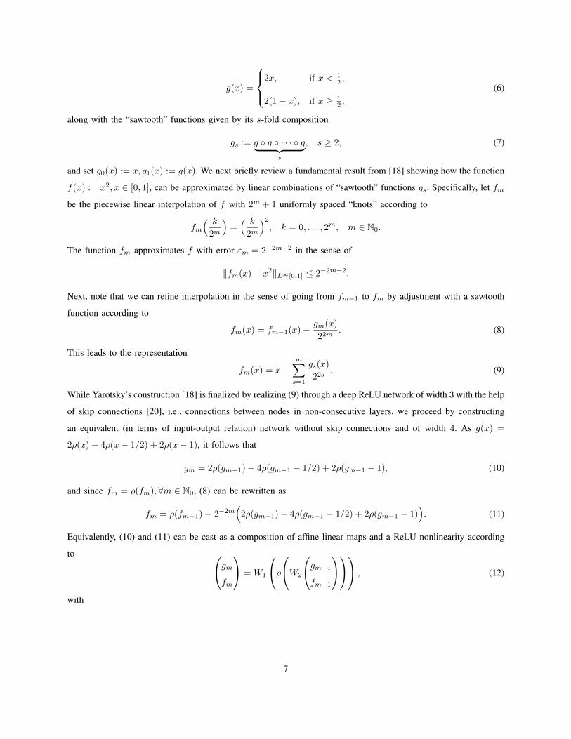
g(x) =
2x, if x < 1
2 ,
2(1− x), if x ≥ 12 ,
(6)
along with the “sawtooth” functions given by its s-fold composition
gs := g g · · · g︸ ︷︷ ︸s
, s ≥ 2, (7)
and set g0(x) := x, g1(x) := g(x). We next briefly review a fundamental result from [18] showing how the function
f(x) := x2, x ∈ [0, 1], can be approximated by linear combinations of “sawtooth” functions gs. Specifically, let fm
be the piecewise linear interpolation of f with 2m + 1 uniformly spaced “knots” according to
fm
( k
2m
)=( k
2m
)2
, k = 0, . . . , 2m, m ∈ N0.
The function fm approximates f with error εm = 2−2m−2 in the sense of
‖fm(x)− x2‖L∞[0,1] ≤ 2−2m−2.
Next, note that we can refine interpolation in the sense of going from fm−1 to fm by adjustment with a sawtooth
function according to
fm(x) = fm−1(x)− gm(x)
22m. (8)
This leads to the representation
fm(x) = x−m∑s=1
gs(x)
22s. (9)
While Yarotsky’s construction [18] is finalized by realizing (9) through a deep ReLU network of width 3 with the help
of skip connections [20], i.e., connections between nodes in non-consecutive layers, we proceed by constructing
an equivalent (in terms of input-output relation) network without skip connections and of width 4. As g(x) =
2ρ(x)− 4ρ(x− 1/2) + 2ρ(x− 1), it follows that
gm = 2ρ(gm−1)− 4ρ(gm−1 − 1/2) + 2ρ(gm−1 − 1), (10)
and since fm = ρ(fm),∀m ∈ N0, (8) can be rewritten as
fm = ρ(fm−1)− 2−2m(
2ρ(gm−1)− 4ρ(gm−1 − 1/2) + 2ρ(gm−1 − 1)). (11)
Equivalently, (10) and (11) can be cast as a composition of affine linear maps and a ReLU nonlinearity according
to gmfm
= W1
ρW2
gm−1
fm−1
, (12)
with
7
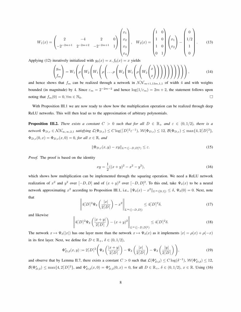
W1(x) =
2 −4 2 0
−2−2m+1 2−2m+2 −2−2m+1 1
x1
x2
x3
x4
, W2(x) =
1 0
1 0
1 0
0 1
x1
x2
−
0
1/2
1
0
. (13)
Applying (12) iteratively initialized with g0(x) = x, f0(x) = x yieldsgmfm
= W1
ρW2
W1
ρ. . . ρ
W2
W1
ρW2
xx
, (14)
and hence shows that fm can be realized through a network in NNm+1,13m,1,1 of width 4 and with weights
bounded (in magnitude) by 4. Since εm = 2−2m−2 and hence log(1/εm) = 2m + 2, the statement follows upon
noting that fm(0) = 0,∀m ∈ N0.
With Proposition III.1 we are now ready to show how the multiplication operation can be realized through deep
ReLU networks. This will then lead us to the approximation of arbitrary polynomials.
Proposition III.2. There exists a constant C > 0 such that for all D ∈ R+ and ε ∈ (0, 1/2), there is a
network ΦD,ε ∈ NN∞,∞,2,1 satisfying L(ΦD,ε) ≤ C log(dDe2ε−1), W(ΦD,ε) ≤ 12, B(ΦD,ε) ≤ max4, 2dDe2,
ΦD,ε(0, x) = ΦD,ε(x, 0) = 0, for all x ∈ R, and
‖ΦD,ε(x, y)− xy‖L∞([−D,D]2) ≤ ε. (15)
Proof. The proof is based on the identity
xy =1
2((x+ y)2 − x2 − y2), (16)
which shows how multiplication can be implemented through the squaring operation. We need a ReLU network
realization of x2 and y2 over [−D,D] and of (x + y)2 over [−D,D]2. To this end, take Ψδ(x) to be a neural
network approximating x2 according to Proposition III.1, i.e., ‖Ψδ(x) − x2‖L∞([0,1]) ≤ δ, Ψδ(0) = 0. Next, note
that ∥∥∥∥∥4dDe2Ψδ
(|x|
2dDe
)− x2
∥∥∥∥∥L∞([−D,D])
≤ 4dDe2δ, (17)
and likewise ∥∥∥∥∥4dDe2Ψδ
(|x+ y|2dDe
)− (x+ y)2
∥∥∥∥∥L∞([−D,D]2)
≤ 4dDe2δ. (18)
The network x 7→ Ψδ(|x|) has one layer more than the network x 7→ Ψδ(x) as it implements |x| = ρ(x) + ρ(−x)
in its first layer. Next, we define for D ∈ R+, δ ∈ (0, 1/2),
Φ∗D,δ(x, y) := 2dDe2(
Ψδ
(|x+ y|2dDe
)−Ψδ
(|x|
2dDe
)−Ψδ
(|y|
2dDe
)), (19)
and observe that by Lemma II.7, there exists a constant C > 0 such that L(Φ∗D,δ) ≤ C log(δ−1), W(Φ∗D,δ) ≤ 12,
B(Φ∗D,δ) ≤ max4, 2dDe2, and Φ∗D,δ(x, 0) = Φ∗D,δ(0, x) = 0, for all D ∈ R+, δ ∈ (0, 1/2), x ∈ R. Using (16)
8
in combination with (17) and (18), we get∥∥∥∥∥Φ∗D,δ(x, y)− 1
2
((x+ y)2 − x2 − y2
)∥∥∥∥∥L∞([−D,D]2)
≤ 6dDe2δ.
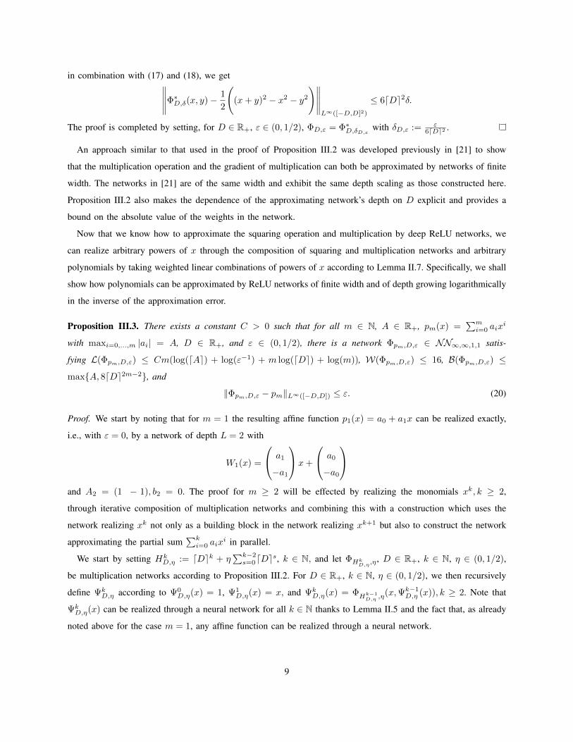
The proof is completed by setting, for D ∈ R+, ε ∈ (0, 1/2), ΦD,ε = Φ∗D,δD,ε with δD,ε := ε6dDe2 .
An approach similar to that used in the proof of Proposition III.2 was developed previously in [21] to show
that the multiplication operation and the gradient of multiplication can both be approximated by networks of finite
width. The networks in [21] are of the same width and exhibit the same depth scaling as those constructed here.
Proposition III.2 also makes the dependence of the approximating network’s depth on D explicit and provides a
bound on the absolute value of the weights in the network.
Now that we know how to approximate the squaring operation and multiplication by deep ReLU networks, we
can realize arbitrary powers of x through the composition of squaring and multiplication networks and arbitrary
polynomials by taking weighted linear combinations of powers of x according to Lemma II.7. Specifically, we shall
show how polynomials can be approximated by ReLU networks of finite width and of depth growing logarithmically
in the inverse of the approximation error.
Proposition III.3. There exists a constant C > 0 such that for all m ∈ N, A ∈ R+, pm(x) =∑mi=0 aix
i
with maxi=0,...,m |ai| = A, D ∈ R+, and ε ∈ (0, 1/2), there is a network Φpm,D,ε ∈ NN∞,∞,1,1 satis-
fying L(Φpm,D,ε) ≤ Cm(log(dAe) + log(ε−1) + m log(dDe) + log(m)), W(Φpm,D,ε) ≤ 16, B(Φpm,D,ε) ≤
maxA, 8dDe2m−2, and
‖Φpm,D,ε − pm‖L∞([−D,D]) ≤ ε. (20)
Proof. We start by noting that for m = 1 the resulting affine function p1(x) = a0 + a1x can be realized exactly,
i.e., with ε = 0, by a network of depth L = 2 with
W1(x) =
a1
−a1
x+
a0
−a0
and A2 = (1 − 1), b2 = 0. The proof for m ≥ 2 will be effected by realizing the monomials xk, k ≥ 2,
through iterative composition of multiplication networks and combining this with a construction which uses the
network realizing xk not only as a building block in the network realizing xk+1 but also to construct the network
approximating the partial sum∑ki=0 aix
i in parallel.
We start by setting HkD,η := dDek + η
∑k−2s=0dDes, k ∈ N, and let ΦHkD,η,η , D ∈ R+, k ∈ N, η ∈ (0, 1/2),
be multiplication networks according to Proposition III.2. For D ∈ R+, k ∈ N, η ∈ (0, 1/2), we then recursively
define ΨkD,η according to Ψ0
D,η(x) = 1, Ψ1D,η(x) = x, and Ψk
D,η(x) = ΦHk−1D,η ,η
(x,Ψk−1D,η (x)), k ≥ 2. Note that
ΨkD,η(x) can be realized through a neural network for all k ∈ N thanks to Lemma II.5 and the fact that, as already
noted above for the case m = 1, any affine function can be realized through a neural network.
9
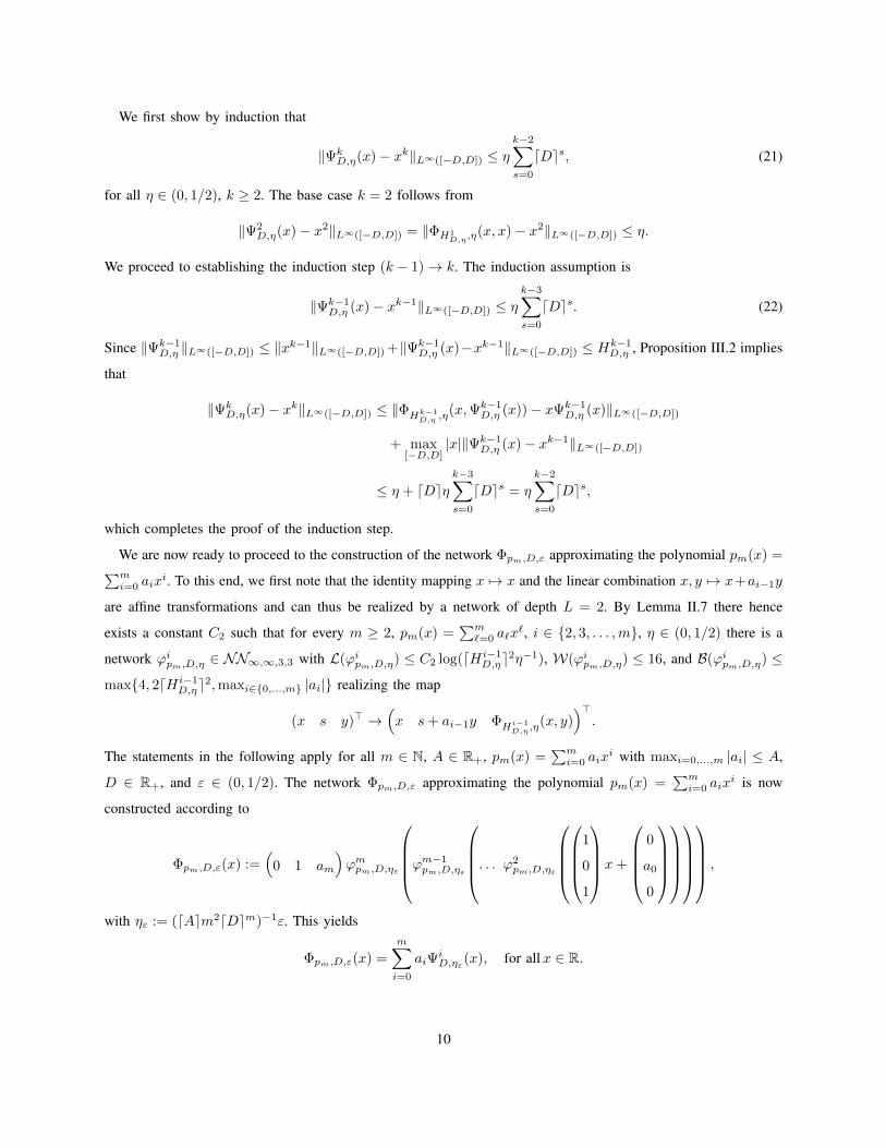
We first show by induction that
‖ΨkD,η(x)− xk‖L∞([−D,D]) ≤ η
k−2∑s=0
dDes, (21)
for all η ∈ (0, 1/2), k ≥ 2. The base case k = 2 follows from
‖Ψ2D,η(x)− x2‖L∞([−D,D]) = ‖ΦH1
D,η,η(x, x)− x2‖L∞([−D,D]) ≤ η.
We proceed to establishing the induction step (k − 1)→ k. The induction assumption is
‖Ψk−1D,η (x)− xk−1‖L∞([−D,D]) ≤ η
k−3∑s=0
dDes. (22)
Since ‖Ψk−1D,η ‖L∞([−D,D]) ≤ ‖xk−1‖L∞([−D,D]) +‖Ψk−1
D,η (x)−xk−1‖L∞([−D,D]) ≤ Hk−1D,η , Proposition III.2 implies
that
‖ΨkD,η(x)− xk‖L∞([−D,D]) ≤ ‖ΦHk−1
D,η ,η(x,Ψk−1
D,η (x))− xΨk−1D,η (x)‖L∞([−D,D])
+ max[−D,D]
|x|‖Ψk−1D,η (x)− xk−1‖L∞([−D,D])
≤ η + dDeηk−3∑s=0
dDes = η
k−2∑s=0
dDes,
which completes the proof of the induction step.
We are now ready to proceed to the construction of the network Φpm,D,ε approximating the polynomial pm(x) =∑mi=0 aix
i. To this end, we first note that the identity mapping x 7→ x and the linear combination x, y 7→ x+ai−1y
are affine transformations and can thus be realized by a network of depth L = 2. By Lemma II.7 there hence
exists a constant C2 such that for every m ≥ 2, pm(x) =∑m`=0 a`x
`, i ∈ 2, 3, . . . ,m, η ∈ (0, 1/2) there is a
network ϕipm,D,η ∈ NN∞,∞,3,3 with L(ϕipm,D,η) ≤ C2 log(dHi−1D,ηe2η−1), W(ϕipm,D,η) ≤ 16, and B(ϕipm,D,η) ≤
max4, 2dHi−1D,ηe2,maxi∈0,...,m |ai| realizing the map
(x s y)> →(x s+ ai−1y ΦHi−1
D,η ,η(x, y)
)>.
The statements in the following apply for all m ∈ N, A ∈ R+, pm(x) =∑mi=0 aix
i with maxi=0,...,m |ai| ≤ A,
D ∈ R+, and ε ∈ (0, 1/2). The network Φpm,D,ε approximating the polynomial pm(x) =∑mi=0 aix
i is now
constructed according to
Φpm,D,ε(x) :=(
0 1 am
)ϕmpm,D,ηε
ϕm−1pm,D,ηε
. . . ϕ2pm,D,ηε
1
0
1
x+
0
a0
0
,
with ηε := (dAem2dDem)−1ε. This yields
Φpm,D,ε(x) =
m∑i=0
aiΨiD,ηε(x), for allx ∈ R.
10
Hence (21) implies∥∥∥Φpm,D,ε(x)− pm∥∥∥L∞([−D,D])
≤m∑i=0
|ai|‖ΨiD,ηε(x)− xi‖L∞([−D,D]) ≤
m∑i=2
|ai|(ηε
i−2∑s=0
dDes)
≤ ηε maxi∈2,...,m
|ai|m∑i=2
(i− 1)dDei−2 ≤ Am2dDem−2ηε ≤ ε.
Thanks to its compositional structure, the width of Φpm,D,ε equals the maximum width of the individual networks
in the composition, i.e., W(Φpm,D,ε) ≤ 16. Since Hi−1D,ηε
≤ 2dDem−1, for i ≤ m, we further have
L(Φpm,D,ε) ≤m∑i=2
L(ϕipm,D,ηε) ≤m∑i=2
C2 log(dHi−1D,ηεe2η−1
ε )
≤ C2m (log(dAe) + log(ε−1) + (3m− 2) log(dDe) + 2 log(m) + 2)
≤ 4C2m (log(dAe) + log(ε−1) +m log(dDe) + log(m)).
Finally, we note that
B(Φpm,D,ε) = max1, |a0|, |am|, maxi∈2,3,...,m
B(ϕipm,D,ηε) ≤ maxA, 8dDe2m−2.
This finalizes the proof.
Next, we recall that the Weierstrass approximation theorem states that every continuous function on a closed
interval can be approximated to within arbitrary accuracy by a polynomial.
Theorem III.4 ([22]). Let [a, b] ⊆ R and f ∈ C([a, b]). Then, for every ε > 0, there exists a polynomial π such
that
‖f − π‖L∞([a,b]) ≤ ε.
Proposition III.3 hence allows to conclude that every continuous function on a closed interval can be approximated
to within arbitrary accuracy by a deep ReLU network of width no more than 16. This amounts to a variant
of the universal approximation theorem [9], [10] for finite-width deep ReLU networks. We note, however, that
the Weierstrass approximation theorem is non-quantitative. A quantitative statement can be obtained for smooth
functions defined as follows.
Definition III.5. For D ∈ R+, let the set SD ⊆ C∞([−D,D],R) be given by
SD =f ∈ C∞([−D,D],R) : ‖f (n)(x)‖L∞([−D,D]) ≤ n!, for all n ∈ N0
. (23)
Lemma III.6. There exist a constant C > 0 and a polynomial π such that for all D ∈ R+, f ∈ SD, and
ε ∈ (0, 1/2), there is a network Ψf,ε ∈ NN∞,∞,1,1 satisfying L(Ψf,ε) ≤ CdDe(log(ε−1))2, W(Ψf,ε) ≤ 23,
B(Ψf,ε) ≤ max1/D, dDeπ(ε−1), and
‖Ψf,ε − f‖L∞([−D,D]) ≤ ε. (24)
11
Proof. We first consider the case D = 1. A fundamental result on Chebyshev interpolation, see e.g. [23, Lemma
3], guarantees, for all f ∈ S1, n ∈ N, the existence of a polynomial Pf,n of degree n such that
‖f − Pf,n‖L∞([−1,1]) ≤ 12n(n+1)!‖f
(n+1)‖L∞([−1,1]) ≤ 12n . (25)
Writing the polynomials Pf,n as Pf,n =∑nj=0 af,n,jx
j , crude—but sufficient for our purposes—estimates show
that there exists a constant c > 0 such that for all f ∈ S1, n ∈ N it holds that
Af,n := maxj=0,...,n
|af,n,j | ≤ 2cn.
Application of Proposition III.3 to Pf,n establishes the existence of a constant C1 > 0 such that for all f ∈ S1,
n ∈ N, ε ∈ (0, 1/2), there is a network ΦPf,n,1,ε/2 ∈ NN∞,∞,1,1 satisfyingW(ΦPf,n,1,ε/2) ≤ 16, B(ΦPf,n,1,ε/2) ≤
maxAf,n, 8 ≤ max2cn, 8,
L(ΦPf,n,1,ε/2) ≤ C1n(cn+ log(2/ε) + log(n)), (26)
and
‖ΦPf,n,1,ε/2 − Pf,n‖L∞([−1,1]) ≤ ε2 . (27)
In the following, we set nε = dlog(2/ε)e and Ψf,ε = ΦPf,nε ,1,ε/2. Combining (25) and (27) establishes that for all
f ∈ S1, ε ∈ (0, 1/2),
‖Ψf,ε − f‖L∞([−1,1]) ≤ ‖Ψf,ε − Pf,nε‖L∞([−1,1]) + ‖Pf,nε − f‖L∞([−1,1])
≤ ε2 + 1
2nε ≤ε2 + ε
2 = ε.
Using dlog(2/ε)e ≤ 2 log(2/ε) and log(2/ε) ≤ 2 log(1/ε), for all ε ∈ (0, 1/2), in (26) implies the existence of a
constant C2 such that for all f ∈ S1, ε ∈ (0, 1/2),
L(Ψf,ε) = L(ΦPf,nε ,1,ε/2) ≤ C2(log(ε−1))2. (28)
By the same token there exists a polynomial π1 such that
B(Ψf,ε) = B(ΦPf,nε ,1,ε/2) ≤ max2cnε , 8 ≤ π1(ε−1).
This completes the proof for the case D = 1.
We next prove the statement for D ∈ (0, 1). To this end, we start by noting that for g ∈ SD, with D ∈ (0, 1),
the function fg : [−1, 1]→ R, x 7→ g(Dx) is in S1. Hence, there exists, for every g ∈ SD, ε ∈ (0, 1/2), a network
Ψfg,ε ∈ NN∞,∞,1,1 satisfying supx∈[−1,1] |Ψfg,ε(x) − fg(x)| ≤ ε, L(Ψfg,ε) ≤ C2(log(1/ε))2, W(Ψfg,ε) ≤ 16,
and B(Ψfg,ε) ≤ π1(ε−1). The claim is established by taking the network approximating g(x) to be Ψ′fg,ε(x) :=
Ψfg,ε(xD ) and noting that
12
supx∈[−D,D]
|Ψ′fg,ε(x)− g(x)| = supx∈[−D,D]
|Ψfg,ε(xD )− fg( xD )|
= supx∈[−1,1]
|Ψfg,ε(x)− fg(x)| ≤ ε,
L(Ψ′fg,ε) ≤ C2(log(1/ε))2, W(Ψ′fg,ε) ≤ 16, and B(Ψfg,ε) ≤ (1/D)π1(ε−1).
It remains to prove the statement for the case D > 1. This will be accomplished by approximating f on intervals
of length 2 (or less) and stitching the resulting approximations together using a localized partition of unity. To
this end consider a, b ∈ R such that 1 ≤ b − a ≤ 2, and let h ∈ C∞([a, b],R) with ‖h(n)‖L∞([a,b]) ≤ n!, for all
n ∈ N0. Next, note that the function x 7→ h(b−a
2 x+ b+a2
)is in S1. Hence, there exists, for every ε ∈ (0, 1/2),
a network Ψ′h,ε ∈ NN∞,∞,1,1 such that supx∈[−1,1] |Ψ′h,ε(x)− h(b−a
2 x+ b+a2
)| ≤ ε, L(Ψ′h,ε) ≤ C2(log(1/ε))2,
W(Ψ′h,ε) ≤ 16, and B(Ψ′h,ε) ≤ π1(ε−1). The networks Ψh,ε(x) := Ψ′h,ε
(2b−ax−
b+ab−a
)then satisfy
supx∈[a,b]
|Ψh,ε(x)− h(x)| = supy∈[−1,1]
|Ψ′h,ε(y)− h(b−a
2 y + b+a2
)| ≤ ε, (29)
L(Ψh,ε) ≤ C2(log(1/ε))2, W(Ψh,ε) ≤ 16, and B(Ψh,ε) ≤ max2, |b|+ |a|π1(ε−1). Now, for D > 1, let ND ∈ N
be such that 1 ≤ 2DND≤ 2 and consider the intervals
ID,k :=[
(k−1)DND
, (k+1)DND
], k ∈ −ND, . . . , ND.
By (29) it follows that, for all D > 1, f ∈ SD, k ∈ −ND, . . . , ND, and ε ∈ (0, 1/2), there exists a network
Ψf,k,ε ∈ NN∞,∞,1,1 satisfying
supx∈ID,k
|Ψf,k,ε(x)− f(x)| ≤ ε4 , (30)
L(Ψf,k,ε) ≤ C2(log(4/ε))2, W(Ψf,k,ε) ≤ 16, and B(Ψf,k,ε) ≤ max2, 2|k|π1(ε−1). We next build a partition of
unity through ReLU networks. Specifically, let χ(x) = ρ(x+ 1)− 2ρ(x) + ρ(x− 1), set χD,k(x) = χ(NDD x− k),
D > 1, k ∈ Z, and note that χD,k ∈ NN2,8,1,1. This yields a partition of unity according to∑k∈Z
χD,k(x) = 1, for allx ∈ R. (31)
For D > 1, f ∈ SD, ε ∈ (0, 1/2), let fε : R→ R be given by
fε(x) :=
ND∑k=−ND
Φ2,ε/4(χD,k(x),Ψf,k,ε(x)), (32)
where Φ2,ε/4 is the multiplication network from Proposition III.2. Note that |f(x)| ≤ 1, for all x ∈ [−D,D], and
|χD,k(x)| ≤ 1, for all x ∈ [−D,D], k ∈ −ND, . . . , ND. Observe further that, for each x ∈ [−D,D], there are
no more than 2 indices k such that χD,k(x) 6= 0. Proposition III.2 therefore implies that the sum in (32) has no
more than 2 non-zero terms for each x ∈ [−D,D]. Combining (30), (31), and Proposition III.2, and noting that
supp(χD,k) = ID,k, hence yields
‖fε − f‖L∞([−D,D]) ≤ ε,
13
for all D > 1, f ∈ SD, ε ∈ (0, 1/2). It remains to show that the functions fε can be realized by networks with
the desired properties. To this end, consider for every D > 1, f ∈ SD, k ∈ 1, . . . , 2ND + 1, ε ∈ (0, 1/2), the
network αf,k,ε ∈ NN∞,∞,1,1 given by
αf,k,ε(x) := Φ2,ε/4(χD,k−(ND+1)(x),Ψf,k−(ND+1),ε(x)),
and the network βf,k,ε ∈ NN∞,∞,3,3 according to
βf,k,ε(x1, x2, x3) :=
x1
αf,k,ε(x2)
x3
.
Further, set β0(x) := (x, 0, 0)T and let A ∈ R3×3 be such that A(y1, y2, y3)T = (y1, y1, y2 + y3)T , for all
y1, y2, y3 ∈ R. We can now define, for every D > 1, f ∈ SD, ε ∈ (0, 1/2), the network Ψf,ε ∈ NN∞,∞,1,1 given
by
Ψf,ε(x) := (0 1 1)βf,2ND+1,ε(Aβf,2ND,ε( . . . (Aβf,1,ε(Aβ0(x))))).
Direct calculation shows that fε(x) = Ψf,ε(x), for all D > 1, f ∈ SD, ε ∈ (0, 1/2), x ∈ R. Furthermore, thanks
to Proposition III.2, there exists a constant C3 > 0 such that, for all D > 1, f ∈ SD, ε ∈ (0, 1/2),
W(Ψf,ε) ≤ 4 + maxk∈1,...,2ND+1
W(αf,k,ε) ≤ 23,
L(Ψf,ε) = 2 +
2ND+1∑k=1
L(βf,k,ε) = 2 +
2ND+1∑k=1
(L(Φ2,ε/4) + maxL(χk−(ND+1)),L(Ψf,k−(ND+1),ε)
)≤ 2 + (2ND + 1)(C1 log(16ε−1) + max2, C2(log(4ε−1))2) ≤ C3D(log(ε−1))2,
and for all f ∈ SD, D ∈ R+, there exists a polynomial π2 so that
B(Ψf,ε) = maxk∈1,...,2ND+1
B(αf,k,ε) ≤ max8, 2D, 4Dπ1(ε−1) ≤ dDeπ2(ε−1). (33)
This concludes the proof.
Remark III.7. Lemma III.6 was formulated for symmetric intervals [−D,D] for the sake of simplicity. The extension
to functions f ∈ C∞([a, b],R) with ‖f (n)‖L∞([a,b]) ≤ n!, for all n ∈ N0, supported on arbitrary intervals [a, b] is
obtained by symmetrizing the support of f according to g(x) = f(x+ b+a2 ) and then applying Lemma III.6 to g(x)
with D = b−a2 . Note that this shift adds a weight of magnitude | b+a2 |, the bounds on L and W remain unaffected.
Remark III.8. The weights of the (finite-width) networks Ψf,ε in Lemma III.6 depending on ε may be undesirable
in practice. Proposition A.1 allows, however, to convert the Ψf,ε into (finite-width) networks with depth still scaling
poly-logarithmically in 1/ε, weights bounded (in absolute value) by 2, and realizing the exact same function. We
14
conclude by noting that the conversion result Proposition A.1 is interesting in its own right as often bounded weights
at the expense of network size are desirable [24].
Remark III.9. The results in this section all have approximating networks of finite width and depth scaling
polylogarithmically in 1/ε. Owing to
M(Φ) ≤ L(Φ)W(Φ)(W(Φ) + 1)
this implies that the connectivity scales no faster than polylogarithmic in 1/ε. It therefore follows that the approx-
imation error ε decays (at least) exponentially fast in the connectivity or equivalently in the number of parameters
the approximant (i.e., the neural network) employs. We say that the network provides exponential approximation
accuracy.
IV. APPROXIMATION OF SINUSOIDAL FUNCTIONS
We are now ready to proceed to the approximation of sinusoidal functions.
Theorem IV.1. There exists a constant C > 0 such that for every a,D ∈ R+, ε ∈ (0, 1/2), there is a network
Ψa,D,ε ∈ NN∞,∞,1,1 satisfying L(Ψa,D,ε) ≤ C((log(1/ε))2 + log(daDe)), W(Ψa,D,ε) ≤ 16, B(Ψa,D,ε) ≤ C,
and
‖Ψa,D,ε − cos(a · )‖L∞([−D,D]) ≤ ε.
Proof. We start by approximating x 7→ cos(2πx) on [0, 1]. To this end note the MacLaurin series representation
cos(x) =
∞∑n=0
(−1)n
(2n)!x2n, ∀x ∈ R.
Thanks to the Taylor theorem with remainder in Lagrange form, we have, for all x ∈ [0, 1],∣∣∣∣∣cos(2πx)−N∑n=0
(−1)n
(2n)!(2πx)2n
∣∣∣∣∣ ≤∣∣∣∣ (2πx)2N+1
(2N + 1)!
∣∣∣∣ supt∈[0,1]
| cos(2N+1)(2πt)| ≤ (2π)4N+2
(2N + 1)!. (34)
Next observe that n! ≥ (ne )ne, for all n ∈ N, which implies,
(2π)4N+2
(2N + 1)!≤ (4π2)2N+1
( 2N+1e )2N+1e
≤( 4π2e
2N + 1
)2N+1
, for allN ∈ N. (35)
With Nε := d2π2e log(2/ε)e, we get, for all ε ∈ (0, 1/2),( 4π2e
2Nε + 1
)2Nε+1
=( 4π2e
2d2π2e log(2/ε)e+ 1
)2d2π2e log(2/ε)e+1
≤ 2−d2π2e log(2/ε)e ≤ 2− log(2/ε) =
ε
2. (36)
Noting that C1 :=⌈maxn∈N0
((2π)2n
(2n)!
)⌉< ∞ and Nε ≤ C2 log(ε−1), for all ε ∈ (0, 1/2), with C2 := 4π2e + 1,
application of Proposition III.3 to
pm(x) = pNε(x) :=
Nε∑n=0
(−1)n
(2n)!(2πx)2n,
with D = 1, establishes the following: There is a constant C3 such that, for all ε ∈ (0, 1/2), there is a network
Φε/2 satisfying
15
∥∥∥Φε/2 − pNε∥∥∥L∞([−1,1])
≤ ε
2, (37)
with W(Φε/2) ≤ 16, B(Φε/2) ≤ C3, and
L(Φε/2) ≤ C3Nε(log(C1) + log(2/ε) +Nε log(1) + log(Nε)) ≤ C4(log(ε−1))2,
where C4 := C2C3(3 + log(C1) + log(C2)). Combining (34), (35), (36), and (37), it follows that the network Φε/2
approximates the function x 7→ cos(2πx) on [0, 1] to within accuracy ε, i.e., for all ε ∈ (0, 1/2), we have
‖Φε/2 − cos(2π · )‖L∞([0,1]) ≤ ε. (38)
We next extend this result to the approximation of x 7→ cos(ax) on the interval [−1, 1] for arbitrary a ∈ R+. This
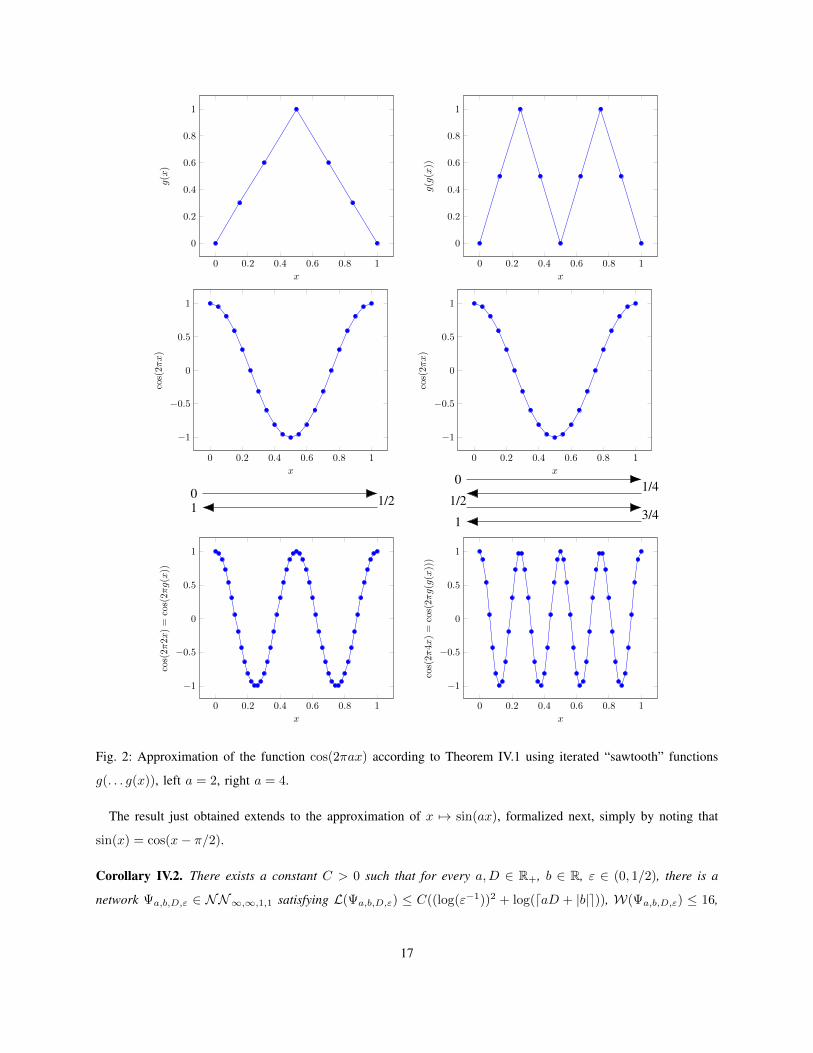
will be accomplished by exploiting that x 7→ cos(2πx) is 1-periodic and even. First recall the “sawtooth” functions
gs : [0, 1]→ [0, 1], s ∈ N, as defined in (7). It is straightforward, albeit somewhat tedious, to see that, for all s ∈ N0,
x ∈ [0, 1],
cos(2π2sx) = cos(2πgs(x)).
Fig. 2 illustrates this relation. Similarly, it follows that cos(2π2sx) = cos(2πgs(|x|)), for all s ∈ N0, x ∈ [−1, 1].
Next, note that for every a ∈ R+, there exists a Ca ∈ (1/2, 1] such that a/(2π) = Ca2dlog(a)−log(2π)e; we thus
have, for all a ∈ R+, x ∈ [−1, 1],
cos(ax) = cos(2π2dlog(a)−log(2π)eCax) = cos(2πgdlog(a)−log(2π)e(Ca|x|)
).
Since gdlog(a)−log(2π)e(Ca|x|) ∈ [0, 1], for all a ∈ R+, x ∈ [−1, 1], it follows from (38) that∥∥∥Φε/2
(gdlog(a)−log(2π)e(Ca|x|)
)− cos
(2πgdlog(a)−log(2π)e(Ca|x|)
)∥∥∥L∞([−1,1])
=∥∥∥Φε/2
(gdlog(a)−log(2π)e(Ca|x|)
)− cos(ax)
∥∥∥L∞([−1,1])
≤ ε.(39)
Now recall that x 7→ |x| = ρ(x) + ρ(−x) can be implemented by a 2-layer network and consider the realization of
x 7→ gdlog(a)−log(2π)e(Cax), a ∈ R+, as developed in the proof of Proposition III.1. Applying Lemma II.5 twice,
then establishes, thanks to (39), the existence of a constant C5 such that the network
Ψa,ε := Φε/2(gdlog(a)−log(2π)e(Ca|x|))
approximates x 7→ cos(ax) on [−1, 1] with accuracy ε, while satisfying L(Ψa,ε) ≤ C5((log(1/ε))2 + log(dae)),
W(Ψa,ε) ≤ 16, and B(Ψa,ε) ≤ C5.
Finally, we consider the approximation of x 7→ cos(ax) on intervals [−D,D], for arbitrary D ≥ 1. To this end,
we define, for all a ∈ R+, D ∈ [1,∞), ε ∈ (0, 1/2), the network Ψa,D,ε(x) := ΨaD,ε(xD ) and observe that
supx∈[−D,D]
|Ψa,D,ε(x)− cos(ax)| = supy∈[−1,1]
|Ψa,D,ε(Dy)− cos(aDy)| = supy∈[−1,1]
|ΨaD,ε(y)− cos(aDy)| ≤ ε.
This concludes the proof.
16
0 0.2 0.4 0.6 0.8 1
0
0.2
0.4
0.6
0.8
1
x
g(x
)
0 0.2 0.4 0.6 0.8 1
0
0.2
0.4
0.6
0.8
1
x
g(g
(x))
0 0.2 0.4 0.6 0.8 1
−1
−0.5
0
0.5
1
x
cos(
2πx
)
0 1/211
0 0.2 0.4 0.6 0.8 1
−1
−0.5
0
0.5
1
x
cos(
2πx
)
0 1/41/2
3/41
0 0.2 0.4 0.6 0.8 1
−1
−0.5
0
0.5
1
x
cos(
2π
2x
)=
cos(
2πg(x
))
0 0.2 0.4 0.6 0.8 1
−1
−0.5
0
0.5
1
x
cos(
2π
4x
)=
cos(
2πg(g
(x))
)
Fig. 2: Approximation of the function cos(2πax) according to Theorem IV.1 using iterated “sawtooth” functions
g(. . . g(x)), left a = 2, right a = 4.
The result just obtained extends to the approximation of x 7→ sin(ax), formalized next, simply by noting that
sin(x) = cos(x− π/2).
Corollary IV.2. There exists a constant C > 0 such that for every a,D ∈ R+, b ∈ R, ε ∈ (0, 1/2), there is a
network Ψa,b,D,ε ∈ NN∞,∞,1,1 satisfying L(Ψa,b,D,ε) ≤ C((log(ε−1))2 + log(daD + |b|e)), W(Ψa,b,D,ε) ≤ 16,
17
B(Ψa,b,D,ε) ≤ C, and
‖Ψa,b,D,ε − cos(a · − b)‖L∞([−D,D]) ≤ ε. (40)
Proof. For given a,D ∈ R+, b ∈ R, ε ∈ (0, 1/2), consider the network Ψa,b,D,ε(x) := Ψa,D+
|b|a ,ε
(x− b
a
)with
Ψa,D,ε as defined in the proof of Theorem IV.1, and observe that
supx∈[−D,D]
|Ψa,b,D,ε(x)− cos(ax− b)| ≤ supy∈[−(D+
|b|a ),D+
|b|a ]|Ψa,D+
|b|a ,ε
(y)− cos(ay)| ≤ ε.
We conclude by noting that both Theorem IV.1 and Corollary IV.2 provide approximation with exponential
accuracy.
V. QUANTIFYING APPROXIMATION QUALITY
We now proceed to developing a framework that allows to formally evaluate the approximation quality achievable
by deep neural networks. The best-known results on approximation by neural networks are the universal approx-
imation theorems of Hornik [10] and Cybenko [9], stating that continuous functions on bounded domains can be
approximated arbitrarily well by a single-hidden-layer (L = 2 in our terminology) neural network with sigmoidal
activation function. The literature on approximation-theoretic properties of networks with a single hidden layer
continuing this line of work is abundant. Without any claim to completeness, we mention work on approximation
error bounds in terms of the number of neurons for functions with bounded first moments [11], [25], the non-
existence of localized approximations [26], a fundamental lower bound on approximation rates [27], [28], and the
approximation of smooth or analytic functions [29], [30].
Approximation-theoretic results for networks with multiple hidden layers were obtained in [31], [32] for general
functions, in [33] for continuous functions, and for functions together with their derivatives in [34]. In [26] it was
shown that for certain approximation tasks deep networks can perform fundamentally better than single-hidden-
layer networks. We also highlight two recent papers, which investigate the benefit—from an approximation-theoretic
perspective—of multiple hidden layers. Specifically, in [35] it was shown that there exists a function which, although
expressible through a small three-layer network, can only be represented through a very large two-layer network;
here size is measured in terms of the total number of neurons in the network.
In the setting of deep convolutional neural networks first results of a nature similar to those in [35] were reported
in [36]. Linking the expressivity properties of neural networks to tensor decompositions, [37], [38] established the
existence of functions that can be realized by relatively small deep convolutional networks but require exponentially
larger shallow convolutional networks.
We conclude by mentioning recent results bearing witness to the approximation power of deep ReLU networks in
the context of PDEs. Specifically, it was shown in [21] that deep ReLU networks can approximate certain solution
18
families of parametric PDEs depending on a large (possibly infinite) number of parameters while overcoming the
curse of dimensionality. The series of papers [39], [40], [41], [42] constructs and analyzes a deep-learning-based
numerical solver for Black-Scholes PDEs that for the first time breaks the curse of dimensionality.
For survey articles on approximation-theoretic aspects of neural networks, we refer the interested reader to [43],
[44]. Most closely related to the framework we develop here is the recent paper by Shaham, Cloninger, and Coifman
[45], which shows that for functions that are sparse in specific wavelet frames, the best M -weight approximation
rate (see Definition V.6 below) of three-layer neural networks is at least as high as the best M -term approximation
rate in piecewise linear wavelet frames.
We begin the development of our framework with a review of a widely used theoretical foundation for deterministic
lossy data compression [46], [47]. Our presentation essentially follows [48], [49].
A. Min-Max (Kolmogorov) Rate Distortion Theory
Let d ∈ N, Ω ⊂ Rd, and consider the function class C ⊂ L2(Ω). Then, for each ` ∈ N, we denote by
E` :=E : C → 0, 1`
the set of binary encoders of C of length `, and we let
D` :=D : 0, 1` → L2(Ω)
be the set of binary decoders of length `. An encoder-decoder pair (E,D) ∈ E` ×D` is said to achieve uniform
error ε over the function class C, if
supf∈C‖D(E(f))− f‖L2(Ω) ≤ ε.
A quantity of central interest is the minimal length ` ∈ N for which there exists an encoder-decoder pair
(E,D) ∈ E` ×D` that achieves uniform error ε over the function class C, along with its asymptotic behavior as
made precise in the following definition.
Definition V.1. Let d ∈ N, Ω ⊂ Rd, and C ⊂ L2(Ω). Then, for ε > 0, the minimax code length L(ε, C) is
L(ε, C) := min
` ∈ N : ∃(E,D) ∈ E` ×D` : sup
f∈C‖D(E(f))− f‖L2(Ω) ≤ ε
.
Moreover, the optimal exponent γ∗(C) is defined as
γ∗(C) := supγ ∈ R : L(ε, C) ∈ O
(ε−1/γ
), ε→ 0
.
The optimal exponent γ∗(C) determines the minimum growth rate of L(ε, C) as the error ε tends to zero and
can hence be seen as quantifying the “description complexity” of the function class C. Larger γ∗(C) results in
smaller growth rate and hence smaller memory requirements for storing signals f ∈ C such that reconstruction with
19
uniformly bounded error is possible. The quantity γ∗(C) is closely related to the concept of Kolmogorov entropy
[50]. Remark 5.10 in [49] makes this connection explicit.
The optimal exponent is known for several function classes, such as subsets of Besov spaces Bsp,q(Rd) with
1 ≤ p, q < ∞, s > 0, and q > (s + 1/2)−1, namely all functions in Bsp,q(Rd) of bounded norm, see e.g. [51].
Specifically, for C a bounded subset of Bsp,q(Rd), γ∗(C) = s/d. Further results are available for β-cartoon-like
functions, which have γ∗(C) = β/2 (see [52], [53]), and for modulation spaces Mp with 1 ≤ p < 2, where
γ∗(C) = 1−1/2+1/p (see [13]).
B. Approximation with Representation Systems
Fix Ω ⊂ Rd. Let C be a compact set of functions in L2(Ω), henceforth referred to as function class, and consider
a corresponding system D := (ϕi)i∈I ⊂ L2(Ω) with I countable, termed representation system. We study the best
M -term approximation error of f ∈ C in D defined as follows.
Definition V.2. [46] Given d ∈ N, Ω ⊂ Rd, a function class C ⊂ L2(Ω), and a representation system D =
(ϕi)i∈I ⊂ L2(Ω), we define, for f ∈ C and M ∈ N,
ΓDM (f) := infIM⊆I,
#IM=M,(ci)i∈IM
∥∥∥∥∥f − ∑i∈IM
ciϕi
∥∥∥∥∥L2(Ω)
. (41)
We call ΓDM (f) the best M -term approximation error of f in D. Every fM =∑i∈IM ciϕi attaining the infimum in
(41) is referred to as a best M -term approximation of f in D. The supremal γ > 0 such that
supf∈C
ΓDM (f) ∈ O(M−γ), M →∞,
will be denoted by γ∗(C,D). We say that the best M -term approximation rate of C in the representation system D
is γ∗(C,D).
Function classes C widely studied in the approximation theory literature include unit balls in Lebesgue, Sobolev,
or Besov spaces [47], as well as α-cartoon-like functions [54]. A wealth of structured representation systems D is
provided by the area of applied harmonic analysis, starting with wavelets [55], followed by ridgelets [28], curvelets
[56], shearlets [57], parabolic molecules [58], and most generally α-molecules [54], which include all previously
named systems as special cases. Further examples are Gabor frames [14], local cosine bases [13], and wave atoms
[15].
The best M -term approximation rate γ∗(C,D) according to Definition V.2 quantifies how difficult it is to
approximate a given function class C in a fixed representation system D. It is sensible to ask whether for given
C, there is a fundamental limit on γ∗(C,D) when one is allowed to vary over D. As shown in [48], [49], every
dense (and countable) D ⊂ L2(Ω), Ω ⊂ Rd, results in γ∗(C,D) =∞ for all function classes C ⊂ L2(Ω). However,
identifying the elements in D participating in the best M -term approximation is practically infeasible as it entails
20
searching through the infinite set D and requires, in general, an infinite number of bits to describe the indices of the
participating elements. This insight leads to the concept of “best M -term approximation subject to polynomial-depth
search” as introduced by Donoho in [48]. Here, the basic idea is to restrict i) the search for the elements in D
participating in the best M -term approximation to the first π(M) elements of D, with π a polynomial, and ii) the
coefficients ci in the best M -term approximation fM =∑i∈IM ciϕi to be uniformly bounded. We formalize this
under the name of effective best M -term approximation as follows.
Definition V.3. Given d ∈ N, Ω ⊂ Rd, a function class C ⊂ L2(Ω), and a representation system D = (ϕi)i∈I ⊂
L2(Ω), the supremal γ > 0 so that there exist a polynomial π and a constant D > 0 such that
supf∈C
infIM⊂1,2,...,π(M),
#IM=M, (ci)i∈IM ,maxi∈IM |ci| ≤D
∥∥∥∥∥f − ∑i∈IM
ciϕi
∥∥∥∥∥L2(Ω)
∈ O(M−γ), M →∞, (42)
will be denoted by γ∗,eff(C,D) and referred to as effective best M -term approximation rate of C in the representation
system D.
We next recall a result from [48], [49] which states that supD⊂L2(Ω) γ∗,eff(C,D) is, indeed, finite under quite
general conditions on C; more specifically, it is upper-bounded by γ∗(C) and hence limited by the “description
complexity” of C. This endows γ∗(C) with operational meaning.
Theorem V.4. [48], [49] Let d ∈ N and Ω ⊂ Rd. The effective best M -term approximation rate of the function
class C ⊂ L2(Ω) in the representation system D ⊂ L2(Ω) satisfies
γ∗,eff(C,D) ≤ γ∗(C).
In light of this result the following definition is natural (see also [49]).
Definition V.5. Let d ∈ N and Ω ⊂ Rd. If the effective best M -term approximation rate of the function class
C ⊂ L2(Ω) in the representation system D ⊂ L2(Ω) satisfies
γ∗,eff(C,D) = γ∗(C),
we say that the function class C is optimally representable by D.
We next outline how the polynomial depth search constraint and the restriction to bounded coefficients ci lead
to rate-distortion-optimal encoder-decoder pairs. The reader is referred to [49] for a rigorous analysis. We start
by noting that, thanks to the polynomial depth search constraint, the indices of the elements of D participating in
the best M -term representation of f can be represented by a total of M log π(M) = CM log(M) bits for some
constant C. The corresponding coefficients ci are quantized by rounding to integer multiples of dM−αe for some
constant α. As the ci are bounded by a universal constant D, this leads to O(Mα) quantization levels and hence
to a total of C ′M log(M) bits, for some constant C ′, needed to store the quantized coefficients. In summary,
21

we have a representation of f by O(M log(M)) bits. An encoder-decoder pair allowing to reconstruct f from a
bitstring of length O(M log(M)) with approximation error ε ∝ M−γ∗,eff(C,D) (see Definition V.3) is described in
[49]. The basic idea is to encode f by concatenating the binary representations of the indices of the participating
elements of D and of the corresponding quantized coefficients such that the decoder can uniquely read them out
from the overall bitstring. The minimax code length corresponding to this encoder-decoder pair scales according to
ε−1/γ∗,eff(C,D) log(ε−1/γ∗,eff(C,D)) ∈ O(ε−1/(γ∗,eff(C,D)−δ)), ε→ 0, for every δ ∈ (0, γ∗,eff(C,D)). By Definition V.1
this leads to γ∗,eff(C,D) − δ ≤ γ∗(C), for every δ ∈ (0, γ∗,eff(C,D)), which is Theorem V.4 as δ can be chosen
arbitrarily small. In particular, the encoder-decoder pair is rate-distortion-optimal if C is optimally representable by
D, i.e., if γ∗,eff(C,D) = γ∗(C).
C. Approximation with Deep Neural Networks
Inspired by the theory of best M -term approximation with representation systems, we now systematically develop
the new concept of best M -weight approximation through neural networks. At the heart of our philosophy lies the
interpretation of the network weights as the counterpart of the coefficients ci in best M -term approximation. In
other words, parsimony in terms of the number of participating elements in a representation system is replaced by
parsimony in terms of network connectivity. Our development will parallel that for best M -term approximation in
the previous section. We start by introducing the concept of best M -weight approximation rate.
Definition V.6. Given d ∈ N, Ω ⊂ Rd, and a function class C ⊂ L2(Ω), we define, for f ∈ C and M ∈ N,
ΓNNM (f) := infΦ∈NN∞,M,d,1
‖f − Φ‖L2(Ω). (43)
We call ΓNNM (f) the best M -weight approximation error of f . The supremal γ > 0 such that
supf∈C
ΓNNM (f) ∈ O(M−γ), M →∞,
will be denoted by γ∗NN (C). We say that the best M -weight approximation rate of C by neural networks is γ∗NN (C).
We emphasize that the infimum in (43) is taken over all networks with fixed input dimension d, no more than
M nonzero (edge and node) weights, and arbitrary depth L. In particular, this means that the infimum is taken
over all possible network topologies and weight choices. The best M -weight approximation rate is fundamental as
it benchmarks all algorithms that map a function f and an ε > 0 to a neural network approximating f with error
no more than ε.
The two restrictions underlying the concept of effective best M -term approximation through representation sys-
tems, namely polynomial depth search and bounded coefficients, are next addressed in the context of approximation
through deep neural networks. We start by noting that the need for the former is obviated by the tree-like-structure
of neural networks. Specifically, a network Φ of connectivity M can not have its width W(Φ) grow faster than
proportional to M . Similarly, the network depth L(Φ) can not grow faster than proportional to M either. As the
22
total number of nonzero weights in the network can not exceed L(Φ)W(Φ)(W(Φ)+1), this yields at most O(M3)
possibilities for the “locations” (in terms of entries in the A` and the b`) of the M nonzero weights. In fact, there
are only O(M2) possibilities for the locations of the M nonzero weights. To see this, first note that N0, NL ≤M
and∑L−1k=1 Nk ≤M . The total number of weights in the network is hence upper-bounded according to
L∑k=1
(NkNk−1 +Nk) ≤L∑k=1
Nk
L∑k=1
Nk−1 +
L∑k=1
Nk ≤ 4M2 + 2M = O(M2). (44)
Encoding the locations of the M non-zero weights hence requires log((M2
M
)) = O(M log(M)) bits. This assumes,
however, that the topology of the network, i.e., the number of layers L and the Nk are known. Proposition V.12 below
shows that the topology can also be encoded with O(M log(M)) bits. In summary, we can therefore conclude that
the tree-like-structure of neural networks automatically guarantees what we had to enforce through the polynomial
depth search constraint in the case of best M -term approximation. Inspection of the approximation results in Section
III reveals that a sublinear growth restriction on L(Φ) as a function of M is natural. Specifically, the approximation
results in Section III all have L(Φ) proportional to a polynomial in log(ε−1). As we are interested in approximation
error decay according to M−γ , see Definition V.6, this suggests to restrict L(Φ) to growth that is polynomial in
log(M). Such a growth behavior, referred to as polylogarithmic in M , will also turn out crucial for allowing rate-
distortion-optimal quantization. More specifically, it will be required for the quantization result in Lemma V.13
to hold in a way that is compatible with the achievability result Proposition V.12. The second restriction made in
the definition of effective best M -term approximation, namely bounded coefficients, will be replaced by a more
generous growth condition on the network weights; specifically, we will allow the magnitude of the weights to
grow polynomially in M . This growth condition will turn out natural in the context of the approximation results we
are interested in and will be seen below to allow rate-distortion-optimal quantization of the network weights. We
remark, however, that Proposition A.1 allows to convert networks with weights growing polynomially in M into
networks with bounded weights at the expense of increased depth, albeit still with depth polylogarithmic in M .
In summary, we will develop the concept of “best M -weight approximation subject to polylogarithmic depth and
polynomial weight growth”.
We start by introducing notation for neural networks with bounded weights.
Definition V.7. Let L,M, d ∈ N and R ∈ R+. Then, we define
NNRL,M,d,1 := Φ ∈ NNL,M,d,1 : B(Φ) ≤ R .
We are now ready to formalize the notion of effective best M -weight approximation rate subject to polylogarithmic
depth and polynomial weight growth.
Definition V.8. Let d ∈ N, Ω ⊂ Rd, and C ⊂ L2(Ω) be a function class. The supremal γ > 0 so that there is a
polynomial π such that
23
supf∈C
infΦ∈NNπ(M)
π(log(M)),M,d,1
‖f − Φ‖L2(Ω) ∈ O(M−γ), M →∞, (45)
is referred to as effective best M -weight approximation rate of C by neural networks and will be denoted by
γ∗,effNN (C).
We next state the equivalent of Theorem V.4 for approximation by deep neural networks. Specifically, we establish
that the optimal exponent γ∗(C) constitutes a fundamental bound on the effective best M -weight approximation
rate of C as well.
Theorem V.9. Let d ∈ N, Ω ⊂ Rd be bounded, and C ⊂ L2(Ω). Then, we have
γ∗,effNN (C) ≤ γ∗(C).
The key ingredients of the proof of Theorem V.9 are developed throughout this section and the formal proof will
be given at the end of the section. Before getting started, we note that, in analogy to Definition V.5, what we just
found suggests the following.
Definition V.10. For d ∈ N and Ω ⊂ Rd bounded, we say that the function class C ⊂ L2(Ω) is optimally
representable by neural networks if
γ∗,effNN (C) = γ∗(C).
It is remarkable that the fundamental limits of effective best M -term approximation through representation systems
and effective best M -edge approximation in neural networks are determined by the same quantity, although the
approximants in the two cases are vastly different. We have linear combinations of elements of a representation
system with the participating functions identified subject to a polynomial-depth search constraint in the former,
and concatenations of affine functions followed by non-linearities under polynomial growth constraints on the
coefficients of the affine functions as well as polylogarithmic growth constraints on the number of concatenations
in the latter case.
We now commence the program developing the proof of Theorem V.9. As in the arguments in the proof sketch
of Theorem V.4 provided at the end of Section V-B, the main idea is to compare the code length corresponding
to the approximating network to the minimax code length of the function class C to be approximated. To this end,
we will need to represent the approximating network’s nonzero weights and its topology, i.e., L, the Nk and the
nonzero weights’ locations as a bitstring. As the weights are real numbers and hence require, in principle, an infinite
number of bits for their binary representations, we will have to suitably quantize them. In particular, the resolution
of the corresponding quantizer will have to increase with decreasing ε. To formalize this idea, we start by defining
the quantization employed.
24
Definition V.11. Let m ∈ N and ε ∈ (0,∞). The network Φ is said to have (m, ε)-quantized weights if all its
weights are elements of 2−mdlog(ε−1)eZ ∩ [−ε−m, ε−m].
A key ingredient of the proof of Theorem V.9 is the following result, which establishes a fundamental lower
bound on the connectivity of networks with quantized weights achieving uniform error ε over a given function class
C.
Proposition V.12. Let d, d′ ∈ N, Ω ⊂ Rd, C ⊂ L2(Ω), and let π be a polynomial. Further, let
Ψ :
(0,
1
2
)× C → NN∞,∞,d,d′
be a map such that for every f ∈ C, ε ∈ (0, 1/2), the network Ψ(ε, f) has (dπ(log(ε−1))e, ε)-quantized weights
and satisfies
supf∈C‖f −Ψ(ε, f)‖L2(Ω) ≤ ε. (46)
Then,
supf∈CM(Ψ(ε, f)) /∈ O
(ε−1/γ
), ε→ 0, for all γ > γ∗(C). (47)
Proof. The proof is by contradiction. Let γ > γ∗(C) and assume that supf∈CM(Ψ(ε, f)) ∈ O(ε−1/γ), ε→ 0. The
contradiction will be effected by constructing encoder-decoder pairs (Eε, Dε) ∈ E`(ε) ×D`(ε) achieving uniform
error ε over C with
`(ε) ≤ C0 · supf∈C
(M(Ψ(ε, f)) log(M(Ψ(ε, f))) + 1) (log(ε−1))q (48)
≤ C0
(ε−1/γ log(ε−1/γ) + 1
)(log(ε−1))q (49)
≤ C1
(ε−1/γ(log(ε−1))q+1 + (log(ε−1))q
)∈ O
(ε−1/ν
), for ε→ 0, (50)
where C0, C1, q > 0 are constants not depending on f, ε and γ > ν > γ∗(C).
We proceed to the construction of the encoder-decoder pairs (Eε, Dε) ∈ E`(ε)×D`(ε), which will be accomplished
by encoding the network topology and the quantized weights in bitstrings of length `(ε) satisfying (48) while
guaranteeing unique reconstruction (of the network). Fix f ∈ C and ε ∈ (0, 1/2). For the sake of notational
simplicity, we set Ψ := Ψ(ε, f), M :=M(Ψ), and L := L(Ψ). Without loss of generality, we assume throughout
that M is a power of 2 and larger than 1. The case M = 0 will be dealt with in Step 1 below. For all M that
are not powers of 2 and for M = 1, we make use of the fact that NNL,M,d,d′ ⊂ NNL,M ′,d,d′ , where M ′ is the
smallest power of 2 larger than M , and we encode the network like an M ′-edge network. Since M < M ′ ≤ 2M ,
this affects `(ε) by a multiplicative constant only.
Recall that the number of nodes in layers 1, . . . , L is denoted by N1, . . . , NL, where d′ = NL, and d = N0 is the
dimension of the input layer (see Definition II.1). We further denote the number of nodes in layer ` = 1, ..., L− 1
associated with edges of nonzero weight in the following layer by N`. It follows that
25
d+ d′ +
L−1∑`=1
N` ≤ M, (51)
where we set M := M + d+ d′. All other nodes do not contribute to the mapping Ψ(x) and can hence be ignored.
Moreover, we can assume that
L ≤ M (52)
as otherwise there would be at least one layer ` ≥ 1 such that A` = 0. As a consequence, the reduced network
x 7→WLρ(WL−1 . . .W`+1ρ(0 · x+ b`)),
realizes the same function as the original network Ψ but has less than L layers. This reduction can be repeated
inductively until the resulting reduced network satisfies (52).
The bitstring representing Ψ is constructed according to the following steps.
Step 1: If M = 0, we encode the network by a single 0. Upon defining 0 log(0) = 0, we then note that (48)
holds trivially and we terminate the encoding procedure. Else, we encode the network connectivity, M , by starting
the overall bitstring with M 1’s followed by a single 0. The length of this bitstring is therefore bounded by M .
Step 2: We continue by encoding the number of layers in the network. Thanks to (52) this requires no more than
dlog(M)e bits. We thus reserve the next dlog(M)e bits for the binary representation of L.
Step 3: Next, we store the dimensions d and d′ of the input and the output layer, respectively, and the numbers
of nodes N`, ` = 1, . . . , L − 1, associated with edges of nonzero weight. As d, d′ ≤ M and N` ≤ M , for
` = 1, . . . , L−1, we can encode (generously) d, d′, and each N` using dlog(M)e bits. For the sake of concreteness,
we first encode d followed by d′ and N1, . . . , NL−1. In total, Step 3 requires a bitstring of length
(L+ 1)dlog(M)e ≤ (M + 1)dlog(M)e.
In combination with Steps 1 and 2 this yields an overall bitstring of length at most
Mdlog(M)e+ 2dlog(M)e+ M. (53)
Step 4: We encode the topology of the graph associated with Ψ and consider only nodes that contribute to the
mapping Ψ(x). To this end, we enumerate the nodes in Ψ by assigning a unique index i—increasing from left to
right in every layer and ranging from 1 to N := d+ d′+∑L−1`=1 N`—to each of these nodes. By (51) each of these
indices can be encoded by a bitstring of length dlog(M)e. We denote the bitstring corresponding to index i by
b(i) ∈ 0, 1dlog(M)e and let n(i) be the number of children of the node with index i, i.e., the number of nodes in
the next layer connected to the node with index i via an edge (of nonzero weight). For each node i = 1, . . . , N , we
form a bitstring of length n(i) · dlog(M)e by concatenating the bitstrings b(j) for all j such that there is an edge
between i and j. We follow this string with an all-zeros bitstring of length dlog(M)e to signal the transition to the
node with index i+ 1. The enumeration is concluded with an all-zeros bitstring of length dlog(M)e signaling that
the last node has been reached. Overall, this yields a bitstring of length
26
N∑i=1
(n(i) + 1) · dlog(M)e < 2Mdlog(M)e, (54)
where we used∑Ni=1 n(i) < M and (51). Combining (53) and (54) it follows that we have encoded the overall
topology of the network Ψ using at most
M + 3Mdlog(M)e+ 2dlog(M)e (55)
bits.
Step 5: We encode the weights of Ψ. By assumption, Ψ has (dπ(log(ε−1))e, ε)-quantized weights, which means
that each weight of Ψ can be represented by no more than Bε := 2(π(log(ε−1)) + 2) log(ε−1) bits. For each
node i = 1, . . . , N , we reserve the first Bε bits to encode its associated node weight and, for each of its children
a bitstring of length Bε to encode the weight corresponding to the edge between that child and its parent node.
Concatenating the results in ascending order of child node indices, we get a bitstring of length (n(i) + 1)Bε for
node i, and an overall bitstring of length
N∑i=1
(n(i) + 1)Bε ≤ 2MBε (56)
representing the weights of the graph associated with the network Ψ. With (55) this shows that the overall number
of bits needed to encode the network topology and weights is no more than
M + 3Mdlog(M)e+ 2dlog(M)e+ 2MBε. (57)
The network can be recovered by sequentially reading out M,L, d, d′, the N`, the topology, and the quantized
weights from the overall bitstring. It is not difficult to verify that the individual steps in the encoding procedure
were crafted such that this yields unique recovery. As (57) can be upper-bounded by
C0M log(M)(log(ε−1))q (58)
for constants C0, q > 0 depending on d, d′, and π only, we have constructed an encoder-decoder pair (Eε, Dε) ∈
E`(ε) ×D`(ε) with `(ε) satisfying (48). This concludes the proof.
The result just established applies to networks that have each weight represented by a finite number of bits scaling
according to (log(ε−1))q , for some q ∈ N, while guaranteeing that the underlying encoder-decoder pair achieves
uniform error ε over C. We next show that such a compatibility is, indeed, possible. Specifically, this requires a
careful interplay between the network’s depth and connectivity scaling, and its weight growth, all as a function of
ε. This delicate balancing will be seen to be met by our assumptions.
Lemma V.13. Let B,L, d, d′, k ∈ N, Ω ⊆ [−B,B]d, ε ∈ (0, 1/2), and M ≤ ε−k. Further, let Φ ∈ NNL,M,d,d′
with B(Φ) ≤ ε−k and let m ∈ N be such that
m ≥ 3kL+ log(max1, B).
27
Then, there exists a network Φ ∈ NNL,M,d,d′ with (m, ε)-quantized weights satisfying
supx∈Ω‖Φ(x)− Φ(x)‖∞ ≤ ε.
Proof. By Definition II.1 there exist integers N0, N1, . . . , NL ∈ N and affine maps
W` : RN`−1 → RN` , x 7→W`(x) = A`x+ b`, ` = 1, 2, . . . , L
with A` ∈ RN`×N`−1 , b` ∈ RN` such that
Φ(x) =
W2(ρ (W1(x))), L = 2
WL(ρ (WL−1(ρ (. . . ρ (W1(x)))))), L ≥ 3.
We now consider the partial networks Φ` : Ω→ RN` , ` ∈ 1, 2, . . . , L− 1, given by
Φ`(x) =
ρ (W1(x)), ` = 1
ρ (W2(ρ (W1(x)))), ` = 2
ρ (W`(ρ (W`−1(. . . ρ (W1(x)))))), ` ≥ 3
and to simplify notation we write ΦL := Φ. Furthermore, for ` ∈ 1, 2, . . . , L, let Φ` be the (partial) network
obtained by replacing all the entries of the A`, b` by a corresponding closest element in 2−mdlog2(ε−1)e Z ∩
[−ε−m, ε−m]. The resulting networks Φ`, ` ∈ 1, 2, . . . , L, are hence defined by matrices A` ∈ RN`×N`−1
and vectors b` ∈ RN` satisfying, for all ` ∈ 1, 2, . . . , L,
maxi,j|A`,i,j − A`,i,j | ≤ 1
22−mdlog2(ε−1)e ≤ 12εm,
maxi,j|b`,i,j − b`,i,j | ≤ 1
22−mdlog2(ε−1)e ≤ 12εm.
(59)
The proof will be effected by upper-bounding the error building up across layers as a result of the quantization of
the edge and node weights. To this end, we define, for ` ∈ 1, 2, . . . , L, the error in the `th layer as
e` := supx∈Ω‖Φ`(x)− Φ`(x)‖∞.
We further set C0 := max1, B and C` := max1, supx∈Ω ‖Φ`(x)‖∞. As each entry of the vector Φ`(x) ∈ RN`
is a weighted sum of at most N`−1 components of the vector Φ`−1(x) ∈ RN`−1 and an affine component b`,i and
B(Φ) ≤ ε−k, by assumption, we have for all ` ∈ 1, 2, . . . , L,
C` ≤ N`−1ε−kC`−1 + ε−k ≤ (N`−1 + 1) ε−kC`−1,
which implies, for all ` ∈ 1, 2, . . . , L, that
C` ≤ C0 ε−k`
`−1∏i=0
(Ni + 1). (60)
28
Next, note that each component (Φ1(x))i, i ∈ 1, 2, . . . , N1, of the vector Φ1(x) ∈ RN1 can be written as
(Φ1(x))i = ρ
N0∑j=1
A1,i,jxj
+ b1,i
,
which, combined with (59) and the fact that ρ is 1-Lipschitz implies
e1 ≤ C0N0εm
2 + εm
2 ≤ C0(N0 + 1) εm
2 . (61)
Similarly, we have for ` ∈ 2, 3, . . . , L, i ∈ 1, 2, . . . , N`,
(Φ`(x))i = ρ
N`−1∑j=1
A`,i,j(Φ`−1(x))j
+ b`,i
,
which implies
e` = supx∈Ω‖Φ`(x)− Φ`(x)‖∞ = sup
x∈Ω,i∈1,...,Nl|(Φ`(x))i − (Φ`(x))i|
= supx∈Ω,i∈1,...,N`
∣∣∣∣∣∣N`−1∑
j=1
A`,i,j(Φ`−1(x))j
+ b`,i
−N`−1∑
j=1
A`,i,j(Φ`−1(x))j
+ b`,i
∣∣∣∣∣∣≤ supx∈Ω,i∈1,...,N`
N`−1∑j=1
∣∣∣A`,i,j(Φ`−1(x))j − A`,i,j(Φ`−1(x))j
∣∣∣+
∣∣∣b`,i − b`,i∣∣∣ .
(62)
Since |(Φ`−1(x))j − (Φ`−1(x))j | ≤ e`−1 and |(Φ`−1(x))j | ≤ C`−1, both for all x ∈ Ω and all j ∈ 1, . . . , N`,
by definition, and |A`,i,j | ≤ ε−k by assumption, upon invoking (59), we get
|A`,i,j(Φ`−1(x))j − A`,i,j(Φ`−1(x))j | ≤ e`−1ε−k + C`−1
εm
2 + e`−1εm
2 .
Since ε ∈ (0, 1/2) it therefore follows from (62), that for all ` ∈ 2, 3, . . . , L,
e` ≤ N`−1(e`−1ε−k + C`−1
εm
2 + e`−1εm
2 ) + εm
2 ≤ (N`−1 + 1)(2e`−1ε−k + C`−1
εm
2 ). (63)
We now claim that, for all ` ∈ 2, 3, . . . , L,
e` ≤ 12 (2` − 1)C0ε
m−(`−1)k`−1∏i=0
(Ni + 1), (64)
which we prove by induction. The base case ` = 1 was already established in (61). For the induction step we
assume that (64) holds for a given ` which, in combination with (60) and (63), implies
e`+1 ≤(N` + 1)(2e`ε
−k + C`εm
2
)≤ (N` + 1)
((2` − 1)C0ε
m−(`−1)kε−k`−1∏i=0
(Ni + 1) + C0ε−k` εm
2
`−1∏i=0
(Ni + 1)
)
=1
2(2`+1 − 1)C0ε
m−`k∏i=0
(Ni + 1).
29
This completes the induction argument and establishes (64). Using 2L−1 ≤ ε−(L−1),∏L−1i=0 (Ni+1) ≤ML ≤ ε−kL,
C0 ≤ ε− log(max1,B), and m ≥ 3kL+ log(max1, B) by assumption, we get
supx∈Ω‖Φ(x)− Φ(x)‖∞ = eL ≤ 1
2 (2L − 1)C0εm−(L−1)k
L−1∏i=0
(Ni + 1)
≤ εm−(L−1+kL−k+log(max1,B)+kL)
≤ εm−(3kL+log(max1,B)−1) ≤ ε.
This completes the proof.
Proposition V.12 not only says that the connectivity growth rate of networks with quantized weights achieving
uniform approximation error ε over a function class C must exceed O(ε−1/γ∗(C)) , ε→ 0, but its proof, by virtue
of constructing an encoder-decoder pair that achieves this growth rate also provides an achievability result. We next
establish a matching strong converse—for networks with polynomially bounded weights—in the sense of showing
that for γ > γ∗(C), the uniform approximation error remains bounded away from zero for infinitely many M ∈ N.
Proposition V.14. Let d ∈ N, Ω ⊂ Rd be bounded, π a polynomial, and C ⊂ L2(Ω). Then, for all C > 0 and
γ > γ∗(C), we have
supf∈C
infΦ∈NNπ(M)
π(log(M)),M,d,1
‖f − Φ‖L2(Ω) ≥ CM−γ , for infinitely many M ∈ N. (65)
Proof. Let γ > γ∗(C). Assume, towards a contradiction, that (65) holds only for finitely many M ∈ N. Then, there
exists a constant C ′ such that the inequality in (65) holds for no M ∈ N and hence there is a constant C so that
supf∈C
infΦ∈NNπ(M)
π(log(M)),M,d,1
‖f − Φ‖L2(Ω) ≤ CM−γ , for all M ∈ N.
Setting Mε := d(ε/(4C))−1/γe, it follows that, for every f ∈ C and every ε ∈ (0, 1/2), there exists a neural
network Φε,f ∈ NN π(Mε)π(log(Mε)),Mε,d,1
such that
‖f − Φε,f‖L2(Ω) ≤ 2 supf∈C
infΦ∈NNπ(Mε)
π(log(Mε)),Mε,d,1
‖f − Φ‖L2(Ω) ≤ 2CM−γε ≤ ε
2.
Next, by Lemma V.13 there exists a polynomial π∗ such that for every f ∈ C, ε ∈ (0, 1/2), there is a network Φε,f
with (dπ∗(log(ε−1))e, ε)-quantized weights satisfying∥∥∥Φε,f − Φε,f
∥∥∥L2(Ω)
≤ ε
2.
Defining
Ψ :
(0,
1
2
)× C → NN∞,∞,d,1, (ε, f) 7→ Φε,f ,
it follows that
supf∈C‖f −Ψ(ε, f)‖L2(Ω) ≤ ε with M(Ψ(ε, f)) ≤Mε ∈ O(ε−1/γ), ε→ 0.
30
The proof is concluded by noting that Ψ(ε, f) violates Proposition V.12.
We are now ready to proceed to the proof of Theorem V.9.
Proof of Theorem V.9. Suppose towards a contradiction that γ∗,effNN (C) > γ∗(C). Let γ ∈
(γ∗(C), γ∗,eff
NN (C))
. Then,
Definition V.8 implies the existence of a polynomial π and a constant C > 0 such that
supf∈C
infΦM∈NNπ(M)
π(log(M)),M,d,1
‖f − ΦM‖L2(Ω) ≤ CM−γ , for all M ∈ N.
This constitutes a contradiction to Proposition V.14.
We conclude this section with a discussion of the conceptual implications of the results established above.
Proposition V.12 combined with Lemma V.13 establishes that neural networks achieving uniform approximation
error ε while having weights that are polynomially bounded in ε−1 and depth growing polylogarithmically in ε−1
cannot exhibit connectivity growth rate smaller than O(ε−1/γ∗(C)), ε→ 0; in other words, a decay of the uniform
approximation error, as a function of M , faster than O(M−γ∗(C)),M →∞, is not possible.
VI. TRANSITIONING FROM REPRESENTATION SYSTEMS TO NEURAL NETWORKS
We next develop a general framework for transferring results on function approximation through representation
systems to results on approximation by neural networks. In particular, we prove that for a given function class C and
an associated representation system D satisfying certain conditions, there exists a neural network with connectivity
O(M) that achieves (up to a multiplicative constant) the same uniform error over C as a best M -term approximation
in D. This will lead to a characterization of function classes C that are optimally representable by neural networks
in the sense of Definition V.10.
We start by defining the effective representability of representation systems through neural networks.
Definition VI.1. Let d ∈ N, Ω ⊆ Rd, and D = (ϕi)i∈N ⊂ L2(Ω) be a representation system. Then, D is
said to be effectively representable by neural networks, if there exists a bivariate polynomial π such that for all
i ∈ N, ε ∈ (0, 1/2) there is a neural network Φi,ε ∈ NN∞,∞,d,1 satisfying M(Φi,ε) ≤ π(log(ε−1), log(i)),
B(Φi,ε) ≤ π(ε−1, i), and
‖ϕi − Φi,ε‖L2(Ω) ≤ ε.
The next result will allow us to conclude that optimality—in the sense of Definition V.5—of a representation
system D for a signal class C combined with effective representability of D by neural networks implies optimal
representability of C by neural networks.
Theorem VI.2. Let d ∈ N, Ω ⊂ Rd be bounded, and consider the function class C ⊂ L2(Ω). Suppose that
the representation system D = (ϕi)i∈N ⊂ L2(Ω) is effectively representable by neural networks. Then, for all
0 < γ < γ∗,eff(C,D), there exist a polynomial π and a map
31
Ψ :
(0,
1
2
)× C → NN∞,∞,d,1,
such that for every f ∈ C, ε ∈ (0, 1/2) the network Ψ(ε, f) has (dπ(log(ε−1))e, ε)-quantized weights while
satisfying ‖f −Ψ(ε, f)‖L2(Ω) ≤ ε, L(Ψ(ε, f)) ≤ π(log(ε−1)), B(Ψ(ε, f)) ≤ π(ε−1), and
M(Ψ(ε, f)) ∈ O(ε−1/γ), ε→ 0, (66)
where the implicit constant in (66) is independent of f . In particular, it holds that
γ∗,effNN (C) ≥ γ∗,eff(C,D).
Remark VI.3. Theorem VI.2 allows to draw the following conclusion. If D optimally represents the function class
C in the sense of Definition V.5, i.e., γ∗,eff(C,D) = γ∗(C), and if it is, in addition, effectively representable by
neural networks in the sense of Definition VI.1, then, thanks to Theorem V.9, which says that γ∗,effNN (C) ≤ γ∗(C), we
have γ∗,effNN (C) = γ∗(C) and hence C is optimally representable by neural networks in the sense of Definition V.10.
Proof of Theorem VI.2. Let γ′ ∈ (γ, γ∗,eff(C,D)). According to Definition V.3, there exist constants C,D ≥ 1 and
a polynomial π1 such that for every f ∈ C, M ∈ N there is a subset If,M ⊂ 1, . . . , π1(M) of cardinality M and
coefficients (cf,i)i∈If,M with maxi∈If,M |cf,i| ≤ D such that∥∥∥∥∥∥f −∑
i∈If,M
cf,iϕi
∥∥∥∥∥∥L2(Ω)
≤ CM−γ′
2. (67)
Let A := max1, |Ω|1/2 and note that we can assume w.l.o.g. that D ≥ C, which, in turn, implies C4DM
−(γ′+1) ≤
1/2. Effective representability of D according to Definition VI.1 therefore ensures the existence of a bivariate
polynomial π2 such that for all M ∈ N, i ∈ If,M , there is a neural network Φi,M ∈ NN∞,∞,d,1 satisfying
‖ϕi − Φi,M‖L2(Ω) ≤C
4DAM−(γ′+1) (68)
with
M(Φi,M ) ≤ π2
(log
((C
4DAM−(γ′+1)
)−1), log(i)
)= π2
((γ′ + 1) log(M) + log( 4DA
C ), log(i)), (69)
B(Φi,M ) ≤ π2
((C
4DAM−(γ′+1)
)−1
, i
)= π2
(4DAC Mγ′+1, i
). (70)
Consider now for f ∈ C, M ∈ N the networks given by
Ψf,M (x) :=∑
i∈If,M
cf,iΦi,M (x).
Thanks to max(If,M ) ≤ π1(M), (69) implies the existence of a polynomial π3 such that L(Ψf,M ) ≤ π3(log(M))
and M(Ψf,M ) ≤Mπ3(log(M)), for all f ∈ C, M ∈ N, and, owing to 68,∥∥∥∥∥∥Ψf,M −∑
i∈If,M
cf,iϕi
∥∥∥∥∥∥L2(Ω)
≤∑
i∈If,M
cf,iC
4DAM−(γ′+1) ≤ CM−γ
′
4A
|If,M |∑i=1
maxi∈If,M |cf,i|MD ≤ CM−γ
′
4A . (71)
32
As the weights of the networks Φi,M are polynomially bounded in i, M and max(If,M ) ≤ π1(M), we can conclude
that the weights of the networks Ψf,M are polynomially bounded in M . Lemma V.13 therefore ensures the existence
of a polynomial π4 such that for all f ∈ C, M ∈ N, there is a network Ψf,M ∈ NN∞,∞,d,1 with (dπ4(log(ε−1))e, ε)-
quantized weights satisfying L(Ψf,M ) = L(Ψf,M ), M(Ψf,M ) =M(Ψf,M ), B(Ψf,M ) ≤ B(Ψf,M ) + CM−γ′
4A , and∥∥∥Ψf,M − Ψf,M
∥∥∥L∞(Ω)
≤ CM−γ′
4A . (72)
As Ω is bounded by assumption, we have∥∥∥Ψf,M − Ψf,M
∥∥∥L2(Ω)
≤ |Ω|1/2∥∥∥Ψf,M − Ψf,M
∥∥∥L∞(Ω)
≤ CM−γ′
4 , (73)
for all f ∈ C, M ∈ N. Combining (73) with (67) and (71), we get, for all f ∈ C, M ∈ N,∥∥∥f − Ψf,M
∥∥∥L2(Ω)
≤
∥∥∥∥∥∥f −∑
i∈If,M
cf,iϕi
∥∥∥∥∥∥L2(Ω)
+
∥∥∥∥∥∥∑
i∈If,M
cf,iϕi −Ψf,M
∥∥∥∥∥∥L2(Ω)
+∥∥∥Ψf,M − Ψf,M
∥∥∥L2(Ω)
≤ CM−γ′.
(74)
For ε ∈ (0, 1/2) and f ∈ C, we now set Mε :=⌈(C/ε)1/γ′
⌉and
Ψ(ε, f) := Ψf,Mε .
Thus, (74) yields
‖f −Ψ(ε, f)‖L2(Ω) ≤ CM−γ′ε ≤ ε. (75)
For the next step, we first note that, for all polynomials π and 0 ≤ m < n,
O(ε−mπ(log(ε−1))) ⊆ O(ε−n), ε→ 0.
Since 1/γ′ < 1/γ this establishes
M(Ψ(ε, f)) ∈ O(Mεπ3(log(Mε))) ⊆ O(ε−1/γ), ε→ 0. (76)
Since Mε and π3 are independent of f , the implicit constant in (76) does not depend on f . By construction
there exist constants c′ and q so that the weights of the networks Ψ(ε, f) can be represented with no more than
dc′(log(ε−1))qe bits. Moreover, there exist a polynomial π5 such that L(Ψ(ε, f)) ≤ π5(log(ε−1)), for all f ∈ C,
ε ∈ (0, 1/2), and a polynomial π6 so that Ψ(ε, f) ∈ NN π6(M(Ψ(ε,f)))π6(log(M(Ψ(ε,f)))),M(Ψ(ε,f),d,1, for all f ∈ C, ε ∈ (0, 1/2).
Therefore, (76) implies
supf∈C
infΦ∈NNπ6(M)
π6(log(M)),M,d,1
‖f − Φ‖L2(Ω) ∈ O(M−γ), M →∞.
Owing to Definition V.8, it therefore holds that
γ∗,effNN (C) ≥ γ∗,eff(C,D),
33
which concludes the proof.
Remark VI.4. We note that Theorem VI.2 continues to hold for Ω = Rn if the elements of D = (ϕi)i∈N are
compactly supported with the size of their support sets growing no more than polynomially in i. The technical
elements required to show this can be found in the context of the approximation of Gabor systems in the proof of
Theorem VIII.3, but are omitted here for ease of exposition.
VII. AFFINE REPRESENTATION SYSTEMS ARE EFFECTIVELY REPRESENTABLE BY NEURAL NETWORKS
We now proceed to showing that a large class of representation systems, namely affine systems, including
wavelets, ridgelets, curvelets, shearlets, and α-molecules, are effectively representable by neural networks. Thanks to
Theorems VI.2 and V.9, this will then allow us to conclude that any function class that is optimally representable—
in the sense of Definition V.5—by an affine system with a suitable generator function is optimally representable
by neural networks in the sense of Definition V.10. By “suitable” we mean that the generator function can be
approximated well by ReLU networks in a sense to be made precise below. Wavelets, for example, provide optimal
representations (i.e., optimal non-linear approximation) of Besov spaces [59]. For concreteness, we consider the
example of spline wavelet systems at the end of this section.
A. Invariance to Affine Transformations
Affine systems consist of translations and dilations of a given generator function. It is therefore important to
understand the impact of these operations on the approximability—by neural networks—of a given function. As
neural networks realize concatenations of affine functions and non-linearities, it is clear that translations and dilations
can be absorbed into the first layer of the network and the transformed function should inherit its approximability
from the generator function. What we will mostly be concerned with is how the weights in the network and its
domain of approximation are affected.
Proposition VII.1. Let d ∈ N, p ∈ [1,∞], and f ∈ Lp(Rd). Assume that there exists a bivariate polynomial π1
such that for all D ∈ R+, ε ∈ (0, 1/2), there is a network ΦD,ε ∈ NN∞,∞,d,1 satisfying
‖f − ΦD,ε‖Lp([−D,D]d) ≤ ε (77)
with M(ΦD,ε) ≤ π1(log(ε−1), log(dDe)). Then, there exists a bivariate polynomial π2 such that for all full-rank
A ∈ Rd×d, e ∈ Rd, E ∈ R+, and η ∈ (0, 1/2), there is a network ΨA,e,E,η ∈ NN∞,∞,d,1 satisfying∥∥∥|det(A)|1p f(A · − e)−ΨA,e,E,η
∥∥∥Lp([−E,E]d)
≤ η
with M(ΨA,e,E,η) ≤ π2(log(η−1), log(dE‖A‖∞ + ‖e‖∞e)). Moreover, if the weights of the networks ΦD,ε
are polynomially bounded in (D, ε−1), then the weights of the networks ΨA,e,E,η are polynomially bounded in
(‖A‖∞, ‖e‖∞, E, η−1).
34
Proof. By a change of variables, we have for every Φ ∈ NN∞,∞,d,1,∥∥∥|det(A)|1p f(A · − e)− |det(A)|
1pΦ(A · − e)
∥∥∥Lp([−E,E]d)
= ‖f − Φ‖Lp(A·[−E,E]d− e). (78)
Furthermore, observe that
A · [−E,E]d − e ⊂ [−(dE‖A‖∞ + ‖e‖∞), (dE‖A‖∞ + ‖e‖∞)]d. (79)
We now set F = ddE‖A‖∞ + ‖e‖∞e and ΨA,e,E,η := |det(A)|1pΦF,η(A · − e) and note that∥∥∥|det(A)|
1p f(A · − e)−ΨA,e,E,η
∥∥∥Lp([−E,E]d)
= ‖f − ΦF,η‖Lp(A·[−E,E]d− e) ≤ ‖f − ΦF,η‖Lp([−F,F ]d) ≤ η,
where we applied the same reasoning as in (78) in the first equality and used (79) in the first inequality and (77)
in the second inequality. The existence of a polynomial π2 such thatM(ΨA,e,E,η) ≤ π2(log(η−1), log(dE‖A‖∞+
‖e‖∞e)) follows by combining the definition of ΨA,e,E,η with the assumptionM(ΦD,ε) ≤ π1(log(ε−1), log(dDe)).
Moreover, we see that if the weights of ΦF,η are polynomially bounded in (F, η−1), then the weights of ΨA,e,E,η
are polynomially bounded in (‖A‖∞, |det(A)|, ‖e‖∞, E, η−1). Since |det(A)| is polynomially bounded in ‖A‖∞, it
follows that the weights of ΨA,e,E,η are polynomially bounded in (‖A‖∞, ‖e‖∞, E, η−1). This yields the claim.
The second auxiliary result we shall need concerns linear combinations of translates of a given function.
Proposition VII.2. Let r, d ∈ N, p ∈ [1,∞], and f ∈ Lp(Rd). Assume that there exists a bivariate polynomial π1
such that for all D ∈ R+, ε ∈ (0, 1/2), there is a network ΦD,ε ∈ NN∞,∞,d,1 satisfying
‖f − ΦD,ε‖Lp([−D,D]d) ≤ ε (80)
with M(ΦD,ε) ≤ π1(log(ε−1), log(dDe)). Then, there exists a bivariate polynomial π2 such that for all c =
(ci)ri=1 ⊂ R, b = (bi)
ri=1 ⊂ Rd , E ∈ R+, and η ∈ (0, 1/2), there is a network Ψc,b,E,η ∈ NN∞,∞,d,1 satisfying∥∥∥∥∥
r∑i=1
cif(· − bi)−Ψc,b,E,η
∥∥∥∥∥Lp([−E,E]d)
≤ η (81)
withM(Ψc,b,E,η) ≤ π2(log(η−1c ), log(Eb)), where Eb = dE+maxi=1,...,r ‖bi‖∞e and ηc = η/max1,
∑ri=1 |ci|.
Moreover, if the weights of the networks ΦD,ε are polynomially bounded in (D, ε−1), then the weights of the networks
Ψc,b,E,η are polynomially bounded in (max1,∑ri=1 |ci|,max1,maxi=1,...,r ‖bi‖∞, E, η−1).
Proof. It follows from assumption (80) that, for all c = (ci)ri=1 ⊂ R, b = (bi)
ri=1 ⊂ Rd, E ∈ R+, and η ∈ (0, 1/2),∥∥∥∥∥
r∑i=1
cif(· − bi)−r∑i=1
ciΦEb,ηc(· − bi)
∥∥∥∥∥Lp([−E,E]d)
≤
(r∑i=1
|ci|
)· ‖f − ΦEb,ηc‖Lp([−(Eb),(Eb)]d) ≤ η.
The network Ψc,b,E,η :=∑ri=1 ciΦEb,ηc(·− bi) thus satisfies (81). The existence of a bivariate polynomial π2 such
that M(Ψc,b,E,η) ≤ π2(log(η−1c ), log(Eb)) follows by combining M(ΦD,ε) ≤ π1(log(ε−1), log(dDe)), which is
35
by assumption, with Lemma II.7. Finally, it follows from Ψc,b,E,η =∑ri=1 ciΦEb,ηc(·−bi) that ΦEb,ηc with weights
polynomially bounded in (Eb, η−1c ) implies Ψc,b,E,η with weights polynomially bounded in(
max
1,
r∑i=1
|ci|
,max
1, maxi=1,...,r
‖bi‖∞, E, η−1
).
B. Affine Representation Systems
We are now ready to introduce the class of representation systems announced above as affine systems. This class
includes all representation systems based on affine transformations of a given generator function. Important special
cases include wavelets, ridgelets, curvelets, shearlets, α-shearlets, and more generally α-molecules.
We proceed to the formal definition of affine systems.
Definition VII.3. Let d, r, S ∈ N, Ω ⊂ Rd be bounded, and f ∈ L∞(Rd) compactly supported. Let δ > 0,
(csk)rk=1 ⊂ R, for s = 0, . . . , S, and (bk)rk=1 ⊂ Rd. Further, let Aj ∈ Rd×d, j ∈ N, be full-rank, with the absolute
values of the eigenvalues of Aj bounded below by 1. Consider the compactly supported functions
gs :=
r∑k=1
cskf(· − bk), s = 0, . . . , S.
We define the affine system D ⊂ L2(Ω) corresponding to (gs)Ss=0 according to
D :=gj,es :=
(|det(Aj)|
12 gs(Aj · − δe)
) ∣∣Ω
: s ∈ 1, 2, . . . , S, e ∈ Zd, j ∈ N, and gj,es 6= 0
∪ ge0 := g0( · − δe)∣∣Ω
: e ∈ Zd and ge0 6= 0,
and refer to f as the generator (function) of D.
We define the sub-systems D0 := ge0 ∈ D : e ∈ Zd and Ds,j := gj,es ∈ D : e ∈ Zd, for s ∈ 1, 2, . . . , S,
j ∈ N. Since every gs, s ∈ 0, 1, . . . , S, has compact support, |D0| and |Ds,j |, for all s = 1, . . . , S and j ∈ N, are
finite. Indeed, we observe that there exists ce := ce(Ω, (gs)Ss=0, δ, d) > 0 such that for all s ∈ 1, . . . , S, j ∈ Z,
and e ∈ Zd,
gj,es ∈ Ds,j =⇒ ‖e‖∞ ≤ ce‖Aj‖∞, and
ge0 ∈ D0 =⇒ ‖e‖∞ ≤ ce.(82)
As all subsystems D0 and Ds,j are finite, we can organize the representation system D according to
D = (ϕi)i∈N = (D0,D1,1, . . . ,DS,1,D1,2, . . . ,DS,2, . . . ) , (83)
where the elements within each sub-system may be ordered arbitrarily. This ordering of D is assumed in the
remainder of the paper and will be referred to as canonical ordering.
36
Moreover, we note that if there exists so ∈ 1, . . . , S such that gso is nonzero, then there is a constant co :=
co(Ω, (gs)Ss=1, δ, d) > 0 such that
S∑s=1
|Ds,j | ≥ co|det(Aj)|, for all j ∈ N. (84)
The next result establishes that affine systems with generator function that can be approximated well by neural
networks are effectively representable by neural networks.
Theorem VII.4. Let d ∈ N, Ω ⊂ Rd be bounded, and D = (ϕi)i∈N ⊂ L2(Ω) an affine system with generator
function f . Assume that there exists a bivariate polynomial π such that for all D ∈ R+, ε ∈ (0, 1/2), there is a
network ΦD,ε ∈ NN∞,∞,d,1 satisfying
‖f − ΦD,ε‖L2([−D,D]) ≤ ε (85)
with M(ΦD,ε) ≤ π(log(ε−1), log(dDe)) and B(ΦD,ε) ≤ π(ε−1, D). Assume furthermore that there exist a, c > 0
such thatj−1∑k=1
|det(Ak)| ≥ c‖Aj‖a∞, for all j ∈ N, j ≥ 2. (86)
Then, D is effectively representable by neural networks.
Proof. Let (gs)Ss=0 be as in Definition VII.3. If gs = 0 for all s ∈ 0, . . . , S, then D = ∅ and the result is trivial.
We can hence assume that there exists at least one s ∈ 0, . . . , S such that gs 6= 0, which, in turn, implies that
(84) holds.
Pick D such that Ω ⊂ [−D,D]d. By Definition VI.1 we need to establish the existence of a bivariate polynomial
π such that for each i ∈ N, η ∈ (0, 1/2), there is a network Φi,η ∈ NN∞,∞,d,1 satisfying
‖ϕi − Φi,η‖L2(Ω) ≤ η (87)
with M(Φi,η) ≤ π(log(η−1), log(i)) and B(Φi,η) ≤ π(η−1, i). Note that the elements of D = (ϕi)i∈N ⊂ L2(Ω)
consist of dilations and translations of f according to
ϕi =(|det(Aji)|
12 gsi(Aji · − δei)
) ∣∣Ω
or ϕi = g0( · − δei)∣∣Ω, (88)
for si ∈ 1, . . . , S, ji ∈ N, and ei ∈ Zd, where
gs :=
r∑k=1
cskf( · − bk), s = 0, . . . , S,
for some r, S ∈ N. Thanks to (85), combining Propositions VII.2 and VII.1 establishes the claim provided that the
quantities
‖Aji‖∞, D, ‖ei‖∞, maxs∈0,...,S
r∑k=1
|csk|, maxk=1,...,r
‖bk‖∞ (89)
are polynomially bounded in i. To see that this is, indeed, the case, we start by noting that ‖ei‖∞ ∈ O(‖Aji‖∞)
thanks to (82). Moreover, since Ω is bounded and r is fixed, the quantities D, maxs∈0,...,S∑rk=1 |csk|, and
37
maxk=1,...,r ‖bk‖∞ do not depend on i. It therefore suffices to establish that ‖Aji‖∞ is polynomially bounded in
i. To this end simply note that thanks to (86) and (84), for all i ∈ N with ji ≥ 2,
c‖Aji‖a∞ ≤ji−1∑k=1
|det(Ak)| ≤ 1c0
ji−1∑k=1
S∑s=1
|Ds,k| ≤ 1c0i,
where the last inequality follows from the fact that ϕi ∈ Dsi,ji for some si. This ensures that
‖Aji‖∞ ≤ ‖A1‖∞ +
(1
c0ci
) 1a
, for all i ∈ N,
thereby completing the proof.
Remark VII.5. Theorem VII.4 is restricted to bounded Ω and compactly supported generator function f for ease
of exposition. It can be extended to Ω = R and generator functions f of unbounded support but sufficiently fast
decay. This extension requires additional technical steps and an alternative definition of canonical ordering. For
conciseness we do not provide the details here, but refer to the proofs of Theorems VIII.3 and VIII.5, which deal
with the corresponding technical aspects in the context of approximation of Gabor systems by neural networks. We
further remark that condition (86) is very weak; in fact, we are not aware of any affine systems in the literature
that would violate it.
We proceed to establishing a remarkable universality and optimality property of neural networks: Neural networks
provide optimal approximations for all function classes that are optimally approximated by affine systems generated
by functions f that can be approximated well by neural networks.
Theorem VII.6. Let d ∈ N, Ω ⊂ Rd be bounded, and D = (ϕi)i∈N ⊂ L2(Ω) an affine system with generator
function f . Assume that there exists a bivariate polynomial π such that for all D ∈ R+, ε ∈ (0, 1/2), there is a
network ΦD,ε ∈ NN∞,∞,d,1 satisfying ‖f − ΦD,ε‖L2([−D,D]) ≤ ε with M(ΦD,ε) ≤ π(log(ε−1), log(dDe)) and
B(ΦD,ε) ≤ π(ε−1, D), and there are constants a, c > 0 such that (86) holds. Then, we have
γ∗,effNN (C) ≥ γ∗,eff(C,D)
for all function classes C ⊆ L2(Ω). In particular, if C is optimally representable by D (in the sense of Definition
V.5), then C is optimally representable by neural networks (in the sense of Definition V.10).
Proof. The first statement follows from Theorems VI.2 and VII.4, the second is by Theorem V.9.
C. Spline wavelets
We next particularize the results developed in the previous two subsections to show that neural networks optimally
represent all function classes that are optimally representable by spline wavelet systems. As spline wavelet systems
have B-splines as generator functions, we start by defining B-splines. For simplicity of exposition, we shall restrict
ourselves to the univariate case throughout.
38
Definition VII.7. Let N1 := χ[0,1] and for m ∈ N, define
Nm+1 := N1 ∗Nm.
We refer to Nm as the univariate cardinal B-spline of order m.
Recognizing that B-splines are piecewise polynomial, we can apply Proposition III.3 to get the following statement
on the approximation of B-splines by deep neural networks.
Lemma VII.8. Let m ∈ N. Then, there exist a constant C > 0 and a polynomial π such that for all D ∈ R+,
ε ∈ (0, 1/2), there is a neural network ΦD,ε ∈ NN∞,∞,1,1 satisfying
‖ΦD,ε −Nm‖L∞([−D,D]) ≤ ε
with M(ΦD,ε) ≤ C(log(ε−1) + log(dDe)) and B(ΦD,ε) ≤ π(D).
Proof. The proof is based on the following representation [60, Eq. 19]
Nm(x) =1
m!
m+1∑k=0
(−1)k
m+ 1
k
ρ((x− k)m).
Note that the spline order m is fixed in the following and we are concerned with the approximating network’s
dependence on D and ε only. Proposition III.3 now ensures the existence of a constant C1 > 0 and a polynomial
π1 such that for all D ∈ R+, ε ∈ (0, 1/2), there is a network ΨD,ε ∈ NN∞,∞,1,1 satisfying
‖ΨD,ε(x)− xm‖L∞([−(D+m+1),D+m+1]) ≤ε
2(m+ 2)
with M(ΨD,ε) ≤ C1(log(ε−1) + log(dDe)) and B(ΨD,ε) ≤ π1(D). Next, define, for D ∈ R+, ε ∈ (0, 1/2), the
network
ΦD,ε :=1
m!
m+1∑k=0
(−1)k
m+ 1
k
ρ(ΨD,ε( · − k))
and note that since the component networks ρ(ΨD,ε( · − k)) simply have one layer more than ΨD,ε( · − k), there
exists a constant C2 such that M(ΦD,ε) ≤ C2(log(ε−1) + log(dDe)). Moreover, thanks to
1
m!
m+ 1
k
=m+ 1
k!(m− k + 1)!≤ 2 (90)
it follows from Lemmata II.5 and II.7 that there exists a polynomial π2 such that B(ΦD,ε) ≤ π2(D).
Finally, since ρ is 1-Lipschitz, we have for all D ∈ R+, ε ∈ (0, 1/2),
‖ΦD,ε −Nm‖L∞([−D,D]) ≤m+1∑k=0
1
m!
m+ 1
k
‖ρ(ΨD,ε( · − k))− ρ(( · − k)m)‖L∞([−D,D])
≤ 2
m+1∑k=0
‖ΨD,ε(x)− xm‖L∞([−(D+m+1),D+m+1]) ≤ ε,
39
where we used (90). This completes the proof.
We are now ready to introduce spline wavelet systems. For k, j ∈ Z, set
Vk := closL2
(span Nm(2kx− j) : j ∈ Z
), (91)
where closL2 denotes closure with respect to L2-norm. Spline spaces Vk, k ∈ Z, constitute a multiresolution analysis
of L2(R) according to
0 ⊂ . . . V−1 ⊂ V0 ⊂ V1 ⊂ · · · ⊂ L2(R).
Moreover, with the orthogonal complements (. . . ,W−1,W0,W1, . . . ) such that Vk+1 = Vk⊕Wk, where ⊕ denotes
the orthogonal sum, we have
L2(R) = V0 ⊕∞⊕k=0
Wk.
Theorem VII.9 ([61, Theorem 1]). Let m ∈ N. The m-th order spline
ψm(x) =1
2m−1
2m−2∑j=0
(−1)jN2m(j + 1)dm
dxmN2m(2x− j), (92)
with support [0, 2m − 1], is a basic wavelet that generates W0 and thereby all the wavelet spaces Wk, k ∈ Z.
Consequently, the set
Wm := ψk,n(x) = 2k/2ψm(2kx− n) : n ∈ Z, k ∈ N0 ∪ φn(x) = Nm(x− n) : n ∈ Z (93)
is a countable complete orthonormal wavelet basis in L2(R).
It remains to establish that the spline wavelet system (93) is an affine system in the sense of Definition VII.3.
To this end, we first devise an alternative representation of (92). Specifically, using the identity [61, Eq. 2.2]
dm
dxmN2m(x) =
m∑j=0
(−1)j
mj
Nm(x− j),
we get
ψm(x) =
3m−1∑n=1
qnNm(2x− n+ 1), (94)
with
qn =(−1)n+1
2m−1
m∑j=0
mj
N2m(n− j).
Combining (94) and the two-scale relation [61, Eq. 1.9]
Nm(x) =
m∑j=0
2−m+1
mj
Nm(2x− j), (95)
we next establish that the spline wavelet system (93) is an affine system in the sense of Definition VII.3 with
generator f(x) = Nm(2x). In particular, in the notation of Definition VII.3, let d = 1, S = 1, r = 4m, δ = 1,
40
c1k =
qk, 1 ≤ k ≤ 3m− 1
0, 3m ≤ k ≤ r,
c0k =
0, 1 ≤ k ≤ 3m− 1
2−m+1
m
k − 3m
, 3m ≤ k ≤ r,
bk =
k−1
2 , 1 ≤ k ≤ 3m− 1
k−3m2 , 3m ≤ k ≤ r
,
(96)
and Aj = 2j−1, for j ∈ N. Then, we have g1 = ψm, g0 = Nm, and the affine system D ⊂ L2(Ω) corresponding
to g1, g0 is
D :=gj,e1 (x) :=
(|Aj |
12 g1(Aj · − δe)
)∣∣∣Ω
: e ∈ Z, j ∈ N, and gj,e1 6= 0
∪ ge0 := g0( · − δe)∣∣Ω
: e ∈ Z and ge0 6= 0
=Wm.
(97)
We have therefore established the following.
Theorem VII.10. Let Ω ⊂ R be bounded and D = (ϕi)i∈N ⊂ L2(Ω) a spline wavelet system according to (97).
Then, all function classes C ⊆ L2(Ω) that are optimally representable by D (in the sense of Definition V.5), are
optimally representable by neural networks (in the sense of Definition V.10).
Proof. Note that (97) is an affine system with generator function f(x) := Nm(2x) in the sense of Definition VII.3
and condition (86) holds for a = 1, and c = 1/2, asj−1∑k=1
2k−1 =
j−2∑k=0
2k = 2j−1 − 1 ≥ 122j−1,
for all j ≥ 2. Now let ΦD,ε be the networks from Lemma VII.8 and consider the networks ΨD,ε(x) := Φ2D,η(2x)
with η := (2D)−12 ε. Then we have for all D ∈ R+, ε ∈ (0, 1/2) that
‖ΨD,ε − f‖L2([−D,D]) ≤ (2D)12 ‖ΨD,ε − f‖L∞([−D,D])
= (2D)12 ‖Φ2D,η(2 · )−Nm(2 · )‖L∞([−D,D])
= (2D)12 ‖Φ2D,η −Nm‖L∞([−2D,2D]) ≤ (2D)
12 η = ε.
Lemma VII.8 further ensures the existence of a constant C ∈ R+ and a polynomial π such that for all D ∈ R+, ε ∈
(0, 1/2) it holds that M(ΨD,ε) ≤ C(log((2D)−12 ε−1) + log(d2De)) and B(ΨD,ε) ≤ π(2D). Thus Theorem VII.6
establishes the claim.
41
VIII. GABOR SYSTEMS
Affine representation systems discussed in the previous section have the affine group underlying as their generating
structure. In this section, we consider Gabor systems [14], which are generated by the Weyl-Heisenberg group [62],
and consist of time-frequency translates of a given generator function. Gabor systems play a fundamental role
in time-frequency analysis [14] and in the study of partial differential equations [63]. We start with the formal
definition of Gabor systems.
Definition VIII.1 (Gabor systems). Let d ∈ N, f ∈ L2(Rd), and x, ξ ∈ Rd. Define the translation operator
Tx : L2(Rd)→ L2(Rd) according to
Txf(t) := f(t− x)
and the modulation operator Mξ : L2(Rd)→ L2(Rd,C) as
Mξf(t) := e2πi〈ξ,t〉f(t).
Let Ω ⊆ Rd, α, β > 0, and g ∈ L2(Rd). The Gabor system G(g, α, β,Ω) ⊆ L2(Ω) is defined as
G(g, α, β,Ω) :=MξTxg
∣∣Ω
: (x, ξ) ∈ αZd × βZd. (98)
In order to be able to talk about representability in the sense of Definition VI.1, we need to order the elements
in G(g, α, β,Ω). To this end, let G0(g, α, β,Ω) := g∣∣Ω and define Gn(g, α, β,Ω), n ∈ N, recursively according
to
Gn(g, α, β,Ω) := MξTxg∣∣Ω
: (x, ξ) ∈ αZd × βZd, ‖x‖∞ ≤ nα, ‖ξ‖∞ ≤ nβ\n−1⋃k=0
Gk(g, α, β,Ω).
We then organize G(g, α, β,Ω) according to
G(g, α, β,Ω) = (G0(g, α, β,Ω), G1(g, α, β,Ω), . . . ), (99)
where the ordering within the sets Gn(g, α, β,Ω) is arbitrary. Note that the specifics of the overall ordering in (99)
are irrelevant as long as G(g, α, β,Ω) = (ϕi)i∈N with ϕi =Mξ(i)Tx(i)g∣∣Ω
is such that ‖x(i)‖∞ and ‖ξ(i)‖∞ do
not grow faster than polynomial in i; this will become apparent in the proof of Theorem VIII.3.
As Gabor systems are built from time-shifted and modulated versions of a generator function, we first establish that
the approximation-theoretic properties of a given function, here the generator function, are inherited by its modulated
versions. Time shifts are dealt with straightforwardly as they can be incorporated into the affine transform in the
first layer of the network.
Lemma VIII.2. Let d ∈ N, f ∈ L2(Rd) ∩ L∞(Rd), and for every D ∈ R+, ε ∈ (0, 1/2), let ΦD,ε ∈ NN∞,∞,d,1be a network satisfying
‖f − ΦD,ε‖L∞([−D,D]d) ≤ ε. (100)
42
Then, there exists a constant C > 0, not depending on d and f , such that for all D ∈ R+, ε ∈ (0, 1/2), ξ ∈ Rd,
there are networks ΦReD,ξ,ε,Φ
ImD,ξ,ε ∈ NN∞,∞,d,1 satisfying
‖Re(Mξf)− ΦReD,ξ,ε‖L∞([−D,D]d) + ‖Im(Mξf)− ΦIm
D,ξ,ε‖L∞([−D,D]d) ≤ 3ε
with
L(ΦReD,ξ,ε),L(ΦIm
D,ξ,ε) ≤ C((log(1/ε))2 + log(ddD‖ξ‖∞e) + (log(dSfe))2) + L(ΦD,ε),
M(ΦReD,ξ,ε),M(ΦIm
D,ξ,ε) ≤ C((log(1/ε))2 + log(ddD‖ξ‖∞e) + (log(dSfe))2 + d) + 4M(ΦD,ε) + 4L(ΦD,ε),
where Sf := max1, ‖f‖L∞(Rd). Moreover, if the weights of the networks ΦD,ε are polynomially bounded in
(D, ε−1), then the weights of the networks ΦReD,ξ,ε,Φ
ImD,ξ,ε are polynomially bounded in (D, ε−1, ‖ξ‖∞).
Proof. All statements in the proof involving ε pertain to ε ∈ (0, 1/2) without explicitly stating this every time. We
start by observing that
Re(Mξf)(t) = cos(2π〈ξ, t〉)f(t)
Im(Mξf)(t) = sin(2π〈ξ, t〉)f(t)
thanks to f ∈ R. Note that for given ξ ∈ Rd, the map t 7→ 〈ξ, t〉 = ξT t = t1ξ1 + · · · + tdξd is simply a linear
transformation. Theorem IV.1 hence guarantees the existence of a constant C1 such that for all D ∈ R+, ξ ∈ Rd,
ε ∈ (0, 1/2), there is a network ΨD,ξ,ε ∈ NN∞,∞,d,1 satisfying
supt∈[−D,D]d
| cos(2π〈ξ, t〉)−ΨD,ξ,ε(t)| ≤ ε6Sf
(101)
with
L(ΨD,ξ,ε) ≤ C1((log(1/ε))2 + (log(Sf ))2 + log(ddD‖ξ‖∞e)), (102)
M(ΨD,ξ,ε) ≤ C1((log(1/ε))2 + (log(Sf ))2 + log(ddD‖ξ‖∞e) + d), (103)
and B(ΨD,ξ,ε) ≤ C1‖ξ‖∞. Moreover, Proposition III.2 guarantees the existence of a constant C2 > 0 such that for
all ε ∈ (0, 1/2), there is a network µε ∈ NN∞,∞,2,1 satisfying
supx,y∈[−Sf−1/2,Sf+1/2]
|µε(x, y)− xy| ≤ ε6 (104)
with
L(µε),M(µε) ≤ C2(log(1/ε) + log(dSfe)) (105)
and B(µε) ≤ max4, 2dSf + 1/2e2. By Lemma II.7, the network Φ(t) := (ΨD,ξ,ε(t),ΦD,ε(t)) ∈ NN∞,∞,d,2satisfies
M(Φ) ≤ 2M(ΨD,ξ,ε) + 2M(ΦD,ε) + 2L(ΨD,ξ,ε) + 2L(ΦD,ε), (106)
43
L(Φ) ≤ maxL(ΨD,ξ,ε),L(ΦD,ε), (107)
and B(Φ) ≤ maxB(ΨD,ξ,ε),B(ΦD,ε). Finally, applying Lemma II.5 to concatenate the networks Φ and µε, we
obtain the network
ΦReD,ξ,ε(t) := µε(Φ(t)) = µε(ΨD,ξ,ε(t),ΦD,ε(t)) ∈ NN∞,∞,d,1
satisfying
M(ΦReD,ξ,ε) ≤ 4M(ΨD,ξ,ε) + 4M(ΦD,ε) + 4L(ΨD,ξ,ε) + 4L(ΦD,ε) + 2M(µε), (108)
and
L(ΦReD,ξ,ε) ≤ maxL(ΨD,ξ,ε),L(ΦD,ε)+ L(µε). (109)
Next, observe that (101) and (104) imply
‖ΦReD,ξ,ε − Re(Mξf)‖L∞([−D,D]d) = ‖µε(ΨD,ξ,ε( · ),ΦD,ε( · ))− cos(2π〈ξ, · 〉)f( · )‖L∞([−D,D]d)
≤ ‖µε(ΨD,ξ,ε( · ),ΦD,ε( · ))−ΨD,ξ,ε( · )ΦD,ε( · )‖L∞([−D,D]d)
+ ‖ΨD,ξ,ε( · )ΦD,ε( · )− cos(2π〈ξ, · 〉)f( · )‖L∞([−D,D]d)
≤ ‖µε(ΨD,ξ,ε( · ),ΦD,ε( · ))−ΨD,ξ,ε( · )ΦD,ε( · )‖L∞([−D,D]d)
+ ‖ΨD,ξ,ε( · )(ΦD,ε( · )− f( · ))‖L∞([−D,D]d)
+ ‖ΨD,ξ,ε( · )f( · )− cos(2π〈ξ, · 〉)f( · )‖L∞([−D,D]d)
≤ ε6 + (1 + ε
6Sf)ε+ ε
6 ≤32ε.
Combining (108), (109), (102), and (105), we can further see that there exists a constant C > 0 such that
L(ΦReD,ξ,ε) ≤ C((log(1/ε))2 + log(ddD‖ξ‖∞e) + (log(dSfe))2) + L(ΦD,ε),
M(ΦReD,ξ,ε) ≤ C((log(1/ε))2 + log(ddD‖ξ‖∞e) + (log(dSfe))2 + d) + 4M(ΦD,ε) + 4L(ΦD,ε).
It finally follows from Lemmata II.5 and II.7, Proposition III.2, and B(ΨD,ξ,ε) ≤ C1‖ξ‖∞ that the weights of ΦReD,ξ,ε
are polynomially bounded in (D, ε−1, ‖ξ‖∞) if the weights of ΦD,ε are polynomially bounded in (D, ε−1). The
results for ΦImD,ξ,ε follow analogously simply by noting that sin(x) = cos(x− π/2). This completes the proof.
Note that Gabor systems necessarily contain complex-valued functions. The theory developed so far applies,
however, to neural networks with real-valued outputs. As evident from the proof of Lemma VIII.2, this is not an
issue when the generator function g is real-valued. For complex-valued generator functions one needs a version
of Proposition III.2 that applies to the multiplication of complex numbers. Thanks to (a + ib)(a′ + ib′) = (aa′ −
bb′) + i(ab′ + a′b) such a network can be constructed by realizing the real and imaginary parts of the product
as a sum of real-valued multiplication networks and then proceeding as in the proof above. We omit the details
as they are straightforward and would not lead to new conceptual insights. Furthermore, an extension—to the
44
complex-valued case—of the concept of (effective) representability according to Definition VI.1 is needed. This is
effected by considering the set of neural networks with 1-dimensional complex-valued output as neural networks
with 2-dimensional real-valued output, i.e., by setting
NNC∞,∞,d,1 := NN∞,∞,d,2,
with the convention that the first component represents the real part and the second the imaginary part.
We proceed to establishing conditions for effective representability of Gabor systems by neural networks.
Theorem VIII.3. Let d ∈ N, Ω ⊆ Rd, α, β > 0, g ∈ L2(Rd)∩L∞(Rd), and let G(g, α, β,Ω) be the corresponding
Gabor system with ordering as defined in (99). Assume that either Ω is bounded or g is compactly supported.
Further, suppose that there exists a polynomial π such that for every D ∈ R+, ε ∈ (0, 1/2), there is a network
ΦD,ε ∈ NN∞,∞,d,1 satisfying
‖g − ΦD,ε‖L∞([−D,D]d) ≤ ε (110)
withM(ΦD,ε) ≤ π(log(ε−1), log(dDe)) and B(ΦD,ε) ≤ π(ε−1, D). Then, G(g, α, β,Ω) is effectively representable
by neural networks.
Proof. First note that owing to (99), we have G(g, α, β,Ω) = (ϕi)i∈N with ϕi =Mξ(i)Tx(i)g ∈ Gn(i)(g, α, β,Ω),
where
‖ξ(i)‖∞ ≤ n(i)β ≤ iβ and ‖x(i)‖∞ ≤ n(i)α ≤ iα. (111)
We start by considering the case where Ω is bounded, i.e., there exists a constant D > 0 such that Ω ⊆ [−D,D]d.
Combining Proposition VII.2 and Lemma VIII.2, with ‖g‖L∞(Rd) considered constant, we can infer the existence of a
multivariate polynomial π1 such that for all i ∈ N, ε ∈ (0, 1/2), there is a network Φi,ε = (ΦRei,ε,Φ
Imi,ε) ∈ NN
C∞,∞,d,1
satisfying
‖Re(Mξ(i)Tx(i)g)− ΦRei,ε‖L∞(Ω) + ‖Im(Mξ(i)Tx(i)g)− ΦIm
i,ε‖L∞(Ω) ≤ (2D)−d2 ε. (112)
with
M(ΦRei,ε),M(ΦIm
i,ε) ≤ π1(log(ε−1), log(‖ξ(i)‖∞), log(‖x(i)‖∞)),
B(ΦRei,ε),B(ΦIm
i,ε) ≤ π1(ε−1, ‖ξ(i)‖∞, ‖x(i)‖∞).
As |z| ≤ |Re(z)|+ |Im(z)|, it follows from (112) that for all i ∈ N, ε ∈ (0, 1/2),
‖ϕi − Φi,ε‖L2(Ω,C) ≤ (2D)d2 ‖ϕi − Φi,ε‖L∞(Ω,C)
≤ (2D)d2
(‖Re(ϕi)− ΦRe
i,ε‖L∞(Ω) + ‖Im(ϕi)− ΦImi,ε‖L∞(Ω)
)≤ ε.
Moreover, (111) implies the existence of a polynomial π2 such that M(ΦRei,ε),M(ΦIm
i,ε) ≤ π2(log(ε−1), log(i)) and
B(ΦRei,ε),B(ΦIm
i,ε) ≤ π2(ε−1, i), for all i ∈ N, ε ∈ (0, 1/2).We can therefore conclude that G(g, α, β,Ω) is effectively
45
representable by neural networks.
We proceed to proving the statement for the case where g is compactly supported. To be concrete, we let
supp(g) ⊆ [−E,E]d with E > 0. This implies
supp(MξTxg) = supp(Txg) ⊆ x+ [−E,E]d ⊆ [−(‖x‖∞ + E), ‖x‖∞ + E]d. (113)
Again, combining Proposition VII.2 and Lemma VIII.2 ensures the existence of a polynomial π3 such that for all
x, ξ ∈ Rd, ε ∈ (0, 1/2), there are networks ΨRex,ξ,ε,Ψ
Imx,ξ,ε ∈ NN∞,∞,d,1 satisfying
‖Re(MξTxg)−ΨRex,ξ,ε‖L∞(Sx) + ‖Im(MξTxg)−ΨIm
x,ξ,ε‖L∞(Sx) ≤ ε2sx
, (114)
with
M(ΨRex,ξ,ε),M(ΨIm
x,ξ,ε) ≤ π3(log(ε−1), log(‖x‖∞), log(‖ξ‖∞)),
B(ΨRex,ξ,ε),B(ΨIm
x,ξ,ε) ≤ π3(ε−1, ‖x‖∞, ‖ξ‖∞),
and where we set Sx := [−(‖x‖∞ + E + 1), ‖x‖∞ + E + 1]d and sx := |Sx|1/2 to simplify notation. As we
want to establish effective representability for general, possibly unbounded, domains Ω, the estimate in (114) is
insufficient. In particular, we have no control over the behavior of the networks ΨRex,ξ,ε,Ψ
Imx,ξ,ε outside the set Sx.
We can, however, construct networks which exhibit the same scaling behavior in terms of M and B, are strictly
supported in Sx, and realize the same output for all inputs in [−(‖x‖∞ + E), ‖x‖∞ + E]d. To this end let, for
y ∈ R+, the network αy ∈ NN2,8,1,1 be given by
αy(t) := ρ(t− (−y − 1))− ρ(t− (−y))− ρ(t− y) + ρ(t− (y + 1)), t ∈ R.
Note that αy(t) = 1 for t ∈ [−y, y], αy(t) = 0 for t /∈ [−y − 1, y + 1], and αy(t) ∈ (0, 1) else. Next, consider, for
x ∈ Rd, the network given by
χx(t) := ρ
([d∑i=1
α‖x‖∞+E(ti)
]− (d− 1)
), t = (t1, t2, . . . , td) ∈ Rd,
and note that
χx(t) = 1, ∀t ∈ [−(‖x‖∞ + E), ‖x‖∞ + E]d
χx(t) = 0, ∀t /∈ [−(‖x‖∞ + E + 1), ‖x‖∞ + E + 1]d
0 ≤ χx(t) ≤ 1, ∀t ∈ Rd.
As the dimension d and E are considered fixed here, there exists a constant C1 such that, for all x ∈ Rd, we have
M(χx) ≤ C1 and B(χx) ≤ C1 max1, ‖x‖∞. Now, let B := max1, ‖g‖L∞(R). Next, by Proposition III.2 there
exists a constant C2 such that, for all x ∈ Rd, ε ∈ (0, 1/2), there is a network µx,ε ∈ NN∞,∞,1,1 satisfying
supy,z∈[−2B,2B]
|µx,ε(y, z)− yz| ≤ ε4sx
, (115)
46
and, for all y ∈ R,
µx,ε(0, y) = µx,ε(y, 0) = 0, (116)
with M(µx,ε) ≤ C2(log(ε−1) + log(sx)) and B(µx,ε) ≤ C2. Again, with E fixed, there exists a constant C3 such
that M(µx,ε) ≤ C3(log(ε−1) + log(‖x‖∞ + 1)), for all x ∈ Rd, ε ∈ (0, 1/2). Let now
ΓRex,ξ,ε := µx,ε(Ψ
Rex,ξ,ε, χx) and ΓIm
x,ξ,ε := µx,ε(ΨImx,ξ,ε, χx). (117)
Using Lemma II.5 along with (114), (115), and (116) establishes the existence of a polynomial π4 such that for all
x, ξ ∈ Rd, ε ∈ (0, 1/2),
‖Re(MξTxg)− ΓRex,ξ,ε‖L∞(Sx) + ‖Im(MξTxg)− ΓIm
x,ξ,ε‖L∞(Sx) ≤ εsx
(118)
and
M(ΓRex,ξ,ε),M(ΓIm
x,ξ,ε) ≤ π4(log(ε−1), log(‖x‖∞), log(‖ξ‖∞)),
B(ΓRex,ξ,ε),B(ΓIm
x,ξ,ε) ≤ π4(ε−1, ‖x‖∞, ‖ξ‖∞).(119)
As MξTxg, ΓRex,ξ,ε, and ΓIm
x,ξ,ε are supported in Sx for all x, ξ ∈ Rd, ε ∈ (0, 1/2), using (116), we get
‖Re(MξTxg)− ΓRex,ξ,ε‖L2(Rd) + ‖Im(MξTxg)− ΓIm
x,ξ,ε‖L2(Rd)
= ‖Re(MξTxg)− ΓRex,ξ,ε‖L2(Sx) + ‖Im(MξTxg)− ΓIm
x,ξ,ε‖L2(Sx)
≤ sx‖Re(MξTxg)− ΓRex,ξ,ε‖L∞(Sx) + sx‖Im(MξTxg)− ΓIm
x,ξ,ε‖L∞(Sx) ≤ ε.
(120)
Consider now, for i ∈ N, ε ∈ (0, 1/2), the complex-valued network Γi,ε ∈ NNC∞,∞,d,1 given by
Γi,ε := (ΓRex(i),ξ(i),ε,Γ
Imx(i),ξ(i),ε)
and note that, for f ∈ L2(Ω,C),
‖f‖L2(Ω,C) =
(∫Ω
|f(t)|2dt) 1
2
=
(∫Ω
|Re(f(t))|2 + |Im(f(t))|2dt) 1
2
=(‖Re(f)‖2L2(Ω) + ‖Im(f)‖2L2(Ω)
) 12
≤ ‖Re(f)‖L2(Ω) + ‖Im(f)‖L2(Ω).
Hence, (120) implies that, for all i ∈ N, ε ∈ (0, 1/2),
‖ϕi − Γi,ε‖L2(Rd,C) = ‖Mξ(i)Tx(i)g − (ΓRex(i),ξ(i),ε,Γ
Imx(i),ξ(i),ε)‖L2(Rd,C) ≤ ε.
Finally, using (111) in (119), it follows that there exists a polynomial π5 such that for all i ∈ N, ε ∈ (0, 1/2), we
have M(ΓRex(i),ξ(i),ε),M(ΓIm
x(i),ξ(i),ε) ≤ π5(log(ε−1), log(i)) and B(ΓRex(i),ξ(i),ε),B(ΓIm
x(i),ξ(i),ε) ≤ π5(ε−1, i), which
establishes effective representability of G(g, α, β,Ω) by neural networks.
We proceed to establishing the central result of this section. To this end, we first recall that according to Theorem
VII.6 neural networks provide optimal approximations for all function classes that are optimally approximated by
47
affine systems (generated by functions f that can be approximated well by neural networks). While this universality
property is significant as it applies to all affine systems, it is perhaps not completely surprising as affine systems
are generated by affine transformations and neural networks consist of concatenations of affine transformations and
non-linearities. Gabor systems, on the other hand, are generated by the Weyl-Heisenberg group, as opposed to the
affine group, and hence exhibit a fundamentally different mathematical structure. The next result shows that neural
networks also provide optimal approximations for all function classes that are optimally approximated by Gabor
systems (generated by functions g that can be approximated well by neural networks).
Theorem VIII.4. Let d ∈ N, Ω ⊆ Rd, α, β > 0, g ∈ L2(Rd)∩L∞(Rd), and let G(g, α, β,Ω) be the corresponding
Gabor system with ordering as defined in (99). Assume that either Ω is bounded or g is compactly supported.
Further, suppose that there exists a polynomial π such that for all D ∈ R+, ε ∈ (0, 1/2), there is a network
ΦD,ε ∈ NN∞,∞,d,1 satisfying
‖g − ΦD,ε‖L∞([−D,D]d) ≤ ε (121)
with M(ΦD,ε) ≤ π(log(ε−1), log(dDe)) and B(ΦD,ε) ≤ π(ε−1, D). Then, for all function classes C ⊆ L2(Ω),
γ∗,effNN (C) ≥ γ∗,eff(C,G(g, α, β,Ω)).
In particular, if C is optimally representable by G(g, α, β,Ω) (in the sense of Definition V.5), then C is optimally
representable by neural networks (in the sense of Definition V.10).
Proof. The first statement follows from Theorems VI.2 and VIII.3, the second is by Theorem V.9.
We complete the program in this section by showing that the Gaussian function satisfies the conditions on the
generator g in Theorem VIII.3. Gaussian functions are widely used generator functions for Gabor systems owing
to their excellent time-frequency localization and their frame-theoretic optimality properties [14]. We hasten to add
that the result below can be extended to sufficiently smooth generator functions g.
Lemma VIII.5. Let d ∈ N and let g ∈ L2(Rd) be given by
g(x) := e−‖x‖22 .
Then, there exist a constant C > 0 and a polynomial π such that for every ε ∈ (0, 1/2), there is a network
Φε ∈ NN∞,∞,d,1 satisfying
‖Φε − g‖L∞(Rd) ≤ ε
with M(Φε) ≤ π(log(ε−1)) and B(Φε) ≤ π(ε−1).
Proof. Observe that g can be written as the composition of the functions g1 : Rd → R+ and g2 : R+ → R given
by
48
g1(x) := ‖x‖22 =
d∑i=1
x2i ,
g2(y) := e−y.
By Proposition III.2 and Lemma II.7 there exist a constant C1 > 0 and a polynomial π1 (note that we consider d
fixed) such that for every D ∈ R+, ε ∈ (0, 1/2), there is a network Ψ1D,ε ∈ NN∞,∞,d,1 satisfying
supx∈[−D,D]d
|Ψ1D,ε − ‖x‖22| ≤ ε
2 (122)
with
M(Ψ1D,ε) ≤ C1(log(ε−1) + log(dDe)),
B(Ψ1D,ε) ≤ π1(dDe).
(123)
Moreover, as | dn
dyn e−y| = |e−y| ≤ 1 for all n ∈ N, y ≥ 0, Lemma III.6 and Remark III.7 imply the existence
of a constant C2 > 0 and a polynomial π2 such that for every D ∈ R+, ε ∈ (0, 1/2), there is a network
Ψ2D,ε ∈ NN∞,∞,1,1 satisfying
supy∈[0,dD2]
|Ψ2D,ε − e−y| ≤ ε
2 (124)
with
M(Ψ2D,ε) ≤ C2dD2e(log(ε−1))2,
B(Ψ2D,ε) ≤ max
dD2
2 ,max 4dD2 , ddD
2
2 eπ2(ε−1).
(125)
By Lemma II.5 there exists for every D ∈ R+, ε ∈ (0, 1/2), a network ΦD,ε ∈ NN∞,∞,d,1 satisfying ΦD,ε(x) =
Ψ2D,ε(Ψ
1D,ε(x)), for x ∈ Rd, with
M(ΦD,ε) ≤ 2(M(Ψ1D,ε) +M(Ψ2
D,ε)),
B(ΦD,ε) = maxB(Ψ1D,ε),B(Ψ2
D,ε).(126)
Setting Dε := log(ε−1), it follows from (123), (125), and (126) that there exists a polynomial π3 such that for all
ε ∈ (0, 1/2), M(ΦDε,ε) ≤ π3(log(ε−1)) and B(ΦDε,ε) ≤ π3(ε−1). As |e−y| ≤ 1 for all y ≥ 0, combining (122)
and (124) yields for all ε ∈ (0, 1/2), x ∈ [−Dε, Dε]d,
|g(x)− ΦDε,ε(x)| = |e−‖x‖22 −Ψ2
Dε,ε(Ψ1Dε,ε(x))|
≤ |e−‖x‖22 − e−Ψ1
Dε,ε(x)|+ |e−Ψ1
Dε,ε(x) −Ψ2
Dε,ε(Ψ1Dε,ε(x))|
≤ ε2 + ε
2 = ε.
(127)
Based on (127), we can now use the same approach as in the proof of Theorem VIII.3 to construct networks Φε
which are supported on [−Dε, Dε]d, where they approximate g to within error ε, and obey M(Φε) ≤ π(log(ε−1))
and B(Φε) ≤ π(ε−1). Together with |g(x)| ≤ ε, for all |x| ∈ Rd\[−Dε, Dε]d, this completes the proof.
49
Remark VIII.6. Note that Lemma VIII.5 establishes an approximation result that is even stronger than what is
required in Theorem VIII.3. Specifically, we construct a neural network which achieves ε-approximation of the
Gaussian function on all of Rd while exhibiting growth rates on M and B that are independent of the domain of
approximation and satisfy the required dependency on the approximation error ε. This construction can be used
to strengthen Theorem VIII.3 to apply to domain Ω = Rd and generator functions of unbounded support, but
sufficiently rapid decay.
Remark VIII.7. The real-valued counterpart of Gabor systems is known as local cosine bases [13], [14] and
consists of cosine-modulated versions of a given generator function. The techniques developed in this section can
be used to show that neural networks also provide optimal approximations for all function classes that are optimally
approximated by local cosine bases (generated by functions that can be approximated well by neural networks).
Gabor systems and local cosine bases provide optimal non-linear approximation of modulation spaces [64], [13].
The mathematical structure underlying modulation spaces is that of the Weyl-Heisenberg group [65] generated by
the time-shift and the frequency-shift operator.
IX. OSCILLATORY TEXTURES AND THE WEIERSTRASS FUNCTION
As mentioned in the introduction, there are functions that are known to be hard to approximate. Specifically, for
the class of oscillatory textures as considered below and for the Weierstrass function, there are no known methods
that achieve exponential accuracy, i.e., an approximation error that decays exponentially in the number of parameters
employed in the approximant. We establish below that deep ReLU networks fill this gap.
Let us start by defining one-dimensional “oscillatory textures” according to [15].
Definition IX.1. Let the sets FD,a, D, a ∈ R+, be given by
FD,a = cos(ag)h : g, h ∈ SD . (128)
The efficient approximation of functions in FD,a with a large represents a notoriously difficult problem due to
the combination of the rapidly oscillating cosine term and the warping g. The best approximation results available
in the literature [15] are based on wave-atom dictionaries∗ and yield low-order polynomial approximation rates. In
what follows we show that finite-width deep networks drastically improve these results to exponential approximation
rates.
Proposition IX.2. There exist a constant C > 0 and a polynomial π such that for all D, a ∈ R+, f ∈ FD,a, and
ε ∈ (0, 1/2), there is a network Γf,ε ∈ NN∞,∞,1,1 satisfying
∗To be precise, the results of [15] are concerned with the two-dimensional case, whereas we focus on the one-dimensional case. Note,
however, that all our results can be readily extended to the multi-dimensional case.
50
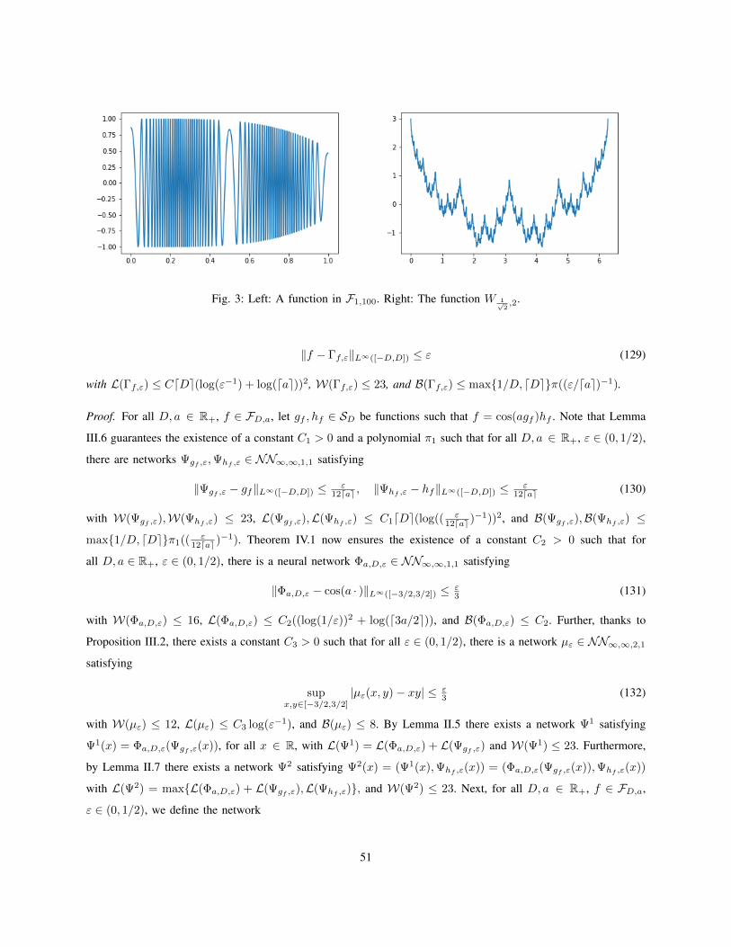
Fig. 3: Left: A function in F1,100. Right: The function W 1√2,2.
‖f − Γf,ε‖L∞([−D,D]) ≤ ε (129)
with L(Γf,ε) ≤ CdDe(log(ε−1) + log(dae))2, W(Γf,ε) ≤ 23, and B(Γf,ε) ≤ max1/D, dDeπ((ε/dae)−1).
Proof. For all D, a ∈ R+, f ∈ FD,a, let gf , hf ∈ SD be functions such that f = cos(agf )hf . Note that Lemma
III.6 guarantees the existence of a constant C1 > 0 and a polynomial π1 such that for all D, a ∈ R+, ε ∈ (0, 1/2),
there are networks Ψgf ,ε,Ψhf ,ε ∈ NN∞,∞,1,1 satisfying
‖Ψgf ,ε − gf‖L∞([−D,D]) ≤ ε12dae , ‖Ψhf ,ε − hf‖L∞([−D,D]) ≤ ε
12dae (130)
with W(Ψgf ,ε),W(Ψhf ,ε) ≤ 23, L(Ψgf ,ε),L(Ψhf ,ε) ≤ C1dDe(log(( ε12dae )
−1))2, and B(Ψgf ,ε),B(Ψhf ,ε) ≤
max1/D, dDeπ1(( ε12dae )
−1). Theorem IV.1 now ensures the existence of a constant C2 > 0 such that for
all D, a ∈ R+, ε ∈ (0, 1/2), there is a neural network Φa,D,ε ∈ NN∞,∞,1,1 satisfying
‖Φa,D,ε − cos(a · )‖L∞([−3/2,3/2]) ≤ ε3 (131)
with W(Φa,D,ε) ≤ 16, L(Φa,D,ε) ≤ C2((log(1/ε))2 + log(d3a/2e)), and B(Φa,D,ε) ≤ C2. Further, thanks to
Proposition III.2, there exists a constant C3 > 0 such that for all ε ∈ (0, 1/2), there is a network µε ∈ NN∞,∞,2,1satisfying
supx,y∈[−3/2,3/2]
|µε(x, y)− xy| ≤ ε3 (132)
with W(µε) ≤ 12, L(µε) ≤ C3 log(ε−1), and B(µε) ≤ 8. By Lemma II.5 there exists a network Ψ1 satisfying
Ψ1(x) = Φa,D,ε(Ψgf ,ε(x)), for all x ∈ R, with L(Ψ1) = L(Φa,D,ε) + L(Ψgf ,ε) and W(Ψ1) ≤ 23. Furthermore,
by Lemma II.7 there exists a network Ψ2 satisfying Ψ2(x) = (Ψ1(x),Ψhf ,ε(x)) = (Φa,D,ε(Ψgf ,ε(x)),Ψhf ,ε(x))
with L(Ψ2) = maxL(Φa,D,ε) + L(Ψgf ,ε),L(Ψhf ,ε), and W(Ψ2) ≤ 23. Next, for all D, a ∈ R+, f ∈ FD,a,
ε ∈ (0, 1/2), we define the network
51
Γf,ε := µε(Ψ2) = µε(Φa,D,ε(Ψgf ,ε),Ψhf ,ε). (133)
Next, by (130), (131), and supx∈R | ddx cos(ax)| = a, we have, for all x ∈ [−D,D],
|Φa,D,ε(Ψgf ,ε(x))− cos(agf (x))| ≤ |Φa,D,ε(Ψgf ,ε(x))− cos(aΨgf ,ε(x))|
+ | cos(aΨgf ,ε(x))− cos(agf (x))|
≤ ε3 + a ε
12dae ≤5ε12 .
Combining this with (130), (132), and ‖ cos ‖L∞([−D,D]), ‖f‖L∞([−D,D]) ≤ 1 yields for all x ∈ [−D,D],
|Γf,ε(x)− f(x)| = |µε(Φa,D,ε(Ψgf ,ε(x)),Ψhf ,ε(x))− cos(agf (x))hf (x)|
≤ |µε(Φa,D,ε(Ψgf ,ε(x)),Ψhf ,ε(x))− Φa,D,ε(Ψgf ,ε(x))Ψhf ,ε(x)|
+ |Φa,D,ε(Ψgf ,ε(x))Ψhf ,ε(x)− cos(agf (x))Ψhf ,ε(x)|
+ | cos(agf (x))Ψhf ,ε(x)− cos(agf (x))hf (x)|
≤ ε3 + 5ε
12
(1 + ε
12dae
)+ ε
12dae ≤ ε.
By Lemma II.5 there exist a constant C4 and a polynomial π2 such that for all D, a ∈ R+, f ∈ FD,a, ε ∈ (0, 1/2),
it holds that W(Γf,ε) ≤ 23,
L(Γf,ε) ≤ L(µε) + maxL(Φa,D,ε) + L(Ψgf ,ε),L(Ψhf ,ε) ≤ C4dDe((log(ε−1) + log(dae))2,
and
B(Γf,ε) ≤ maxB(µε),B(Φa,D,ε),B(Ψgf ,ε),B(Ψhf ,ε) ≤ max1/D, dDeπ2((ε/dae)−1).
This completes the proof.
Finally, we show how the Weierstrass function—a fractal function, which is continuous everywhere but dif-
ferentiable nowhere—can be approximated with exponential accuracy by deep ReLU networks. Specifically, we
consider
Wp,a(x) =
∞∑k=0
pk cos(akπx), for p ∈ (0, 1/2), a ∈ R+, with ap ≥ 1. (134)
Let α = − log(p)log(a) . It is well known [66] that Wp,a possesses Holder smoothness α which may be made arbitrarily
small by suitable choice of a, see Figure 3 right. While classical approximation methods therefore achieve polynomial
approximation rates only, it turns out that finite-width deep networks yield exponential approximation rates. This
is formalized as follows.
Proposition IX.3. There exists a constant C > 0 such that, for all ε, p ∈ (0, 1/2), D, a ∈ R+, there is a network
Ψp,a,D,ε ∈ NN∞,∞,1,1 satisfying
‖Ψp,a,D,ε −Wp,a‖L∞([−D,D]) ≤ ε (135)
52
with
L(Ψp,a,D,ε) ≤ C((log(1/ε))3 + (log(1/ε))2 log(dae) + log(1/ε) log(dDe)),
W(Ψp,a,D,ε) ≤ 20, and B(Ψp,a,D,ε) ≤ C.
Proof. For every N ∈ N, p ∈ (0, 1/2), a ∈ R+, x ∈ R, let SN,p,a(x) =∑Nk=0 p
k cos(akπx) and note that
|SN,p,a(x)−Wp,a(x)| ≤∞∑
k=N+1
|pk cos(akπx)| ≤∞∑
k=N+1
pk = 11−p −
1−pN+1
1−p ≤ 2−N . (136)
Let Nε := dlog(2/ε)e, ε ∈ (0, 1/2). Next note that Theorem IV.1 ensures the existence of a constant C1 > 0 such
that for all D, a ∈ R+, k ∈ N0, ε ∈ (0, 1/2), there is a network φak,D,ε ∈ NN∞,∞,1,1 satisfying
‖φak,D,ε − cos(akπ · )‖L∞([−D,D]) ≤ ε4 (137)
with W(φak,D,ε) ≤ 16, L(φak,D,ε) ≤ C1((log(ε−1))2 + log(dakπDe)), and B(φak,D,ε) ≤ C1. Thanks to x =
ρ(x) − ρ(−x), there exists a neural network τ ∈ NN2,4,1,1 satisfying τ(x) = x, for all x ∈ R. Applying Lemma
II.5 to τ and φak,D,ε, k ≥ 0, we obtain that for all p ∈ (0, 1/2), D, a ∈ R+, k ∈ N0, ε ∈ (0, 1/2), there exist
networks
ψp,a,0D,ε (x) =
x
p0φa0,D,ε(x)
0
and ψp,a,kD,ε (x1, x2, x3) =
x1
pkφak,D,ε(x2)
x3
, k > 0. (138)
Now let A ∈ R3×3 be such that A(y1, y2, y3)T = (y1, y1, y2 +y3)T , for all y ∈ R3. Applying now, for p ∈ (0, 1/2),
D, a ∈ R+, ε ∈ (0, 1/2), Lemma II.5, we obtain that there exist a network Ψp,a,D,ε given by
Ψp,a,D,ε(x) :=(
0 1 1)ψp,a,NεD,ε (Aψp,a,Nε−1
D,ε (. . . (Aψp,a,0D,ε (x)))). (139)
With (137) we get, for all p ∈ (0, 1/2), D, a ∈ R+, ε ∈ (0, 1/2), x ∈ [−D,D],
|Ψp,a,D,ε(x)− SNε,p,a(x)| =
∣∣∣∣∣Nε∑k=0
pkφak,D,ε(x)−Nε∑k=0
pk cos(akπx)
∣∣∣∣∣≤
Nε∑k=0
pk|φak,D,ε(x)− cos(akπx)| ≤ ε4
Nε∑k=0
2−k ≤ ε2 .
Combining this with (136) establishes that for all p ∈ (0, 1/2), D, a ∈ R+, ε ∈ (0, 1/2), x ∈ [−D,D],
|Ψp,a,D,ε(x)−Wp,a(x)| ≤ 2−dlog( 2ε )e + ε
2 ≤ε2 + ε
2 = ε.
The proof is now completed by noting that there exists a constant C2 such that for all p ∈ (0, 1/2), D, a ∈ R+,
ε ∈ (0, 1/2), we have W(Ψp,a,D,ε) ≤ 20,
L(Ψp,a,D,ε) ≤Nε∑k=0
L(φak,D,ε) ≤ (Nε + 1)C1((log(ε−1))2 + log(daNεπDe))
≤ C2((log(ε−1))3 + (log(ε−1))2 log(dae) + log(ε−1) log(dDe)),
53
and
B(Ψp,a,D,ε) = maxk∈0,...,Nε
B(φak,D,ε) ≤ C1.
We finally note that the restriction p ∈ (0, 1/2) was made for simplicity of exposition and can be relaxed to
p ∈ (0, r) with r ∈ (0, 1). For p → 1 the convergence of the sum defining Wp,a can become arbitrarily slow,
leading to issues that are not specific to the approximation of Wp,a by neural networks.
X. IMPOSSIBILITY RESULTS FOR FINITE-DEPTH NETWORKS
This section makes a formal case for deep networks by establishing that, for non-constant periodic functions,
finite-width deep networks require asymptotically—in the function’s “highest frequency”—smaller connectivity than
finite-depth wide networks. This statement is then extended to sufficiently smooth non-periodic functions, thereby
formalizing the benefit of deep networks over shallow networks for the approximation of a broad class of functions.
We start with preparatory material taken from [19].
Definition X.1 ([19]). Let k ∈ N. A function f : R→ R is called k-sawtooth if it is piecewise linear with no more
than k pieces, i.e., its domain R can be partitioned into k intervals such that f is linear on each interval.
Lemma X.2 ([19]). Every Φ ∈ NN∞,∞,1,1 is (2W(Φ))L(Φ)-sawtooth.
Definition X.3. For a u-periodic function f ∈ C(R), we define
ξ(f) := supδ∈[0,u)
infc,d∈R
‖f(x)− (cx+ d)‖L∞([δ,δ+u]).
The quantity ξ(f) measures the error incurred by the best linear approximation of f on any segment of length
equal to the period of f ; ξ(f) can hence be interpreted as quantifying the non-linearity of f . The next result
states that finite-depth networks with width scaling poly-logarithmically in the “highest frequency” of the periodic
function to be approximated can not achieve arbitrarily small approximation error.
Proposition X.4. Let f ∈ C(R) be a non-constant u-periodic function, L ∈ N, and π a polynomial. Then, there
exists an a ∈ N such that for every network Φ ∈ NNL,∞,1,1 with W(Φ) ≤ π(log(a)),
‖f(a · )− Φ‖L∞([0,u]) ≥ ξ(f) > 0.
Proof. First note that there exists an even a ∈ N such that a/2 > (2π(log(a)))L. Lemma X.2 now implies that
every network Φ ∈ NNL,∞,1,1 with W(Φ) ≤ π(log(a)) is (2π(log(a)))L-sawtooth and therefore consists of at
most a/2 different linear pieces. Hence, there exists an interval [u1, u2] ⊆ [0, u] with u2 − u1 ≥ (2u/a) on which
Φ is linear. Since u2− u1 ≥ (2u/a) the interval supports two full periods of f(a · ) and we can therefore conclude
that
54
‖f(a · )− Φ‖L∞([0,u]) ≥ ‖f(a · )− Φ‖L∞([u1,u2]) ≥ infc,d∈R
‖f(x)− (cx+ d)‖L∞([0,2u])
≥ supδ∈[0,u)
infc,d∈R
‖f(x)− (cx+ d)‖L∞([δ,u+δ]) = ξ(f).
Finally note that ξ(f) > 0 as ξ(f) = 0 for u-periodic f ∈ C(R) would entail that f is constant thereby contradicting
the assumption.
Application of Proposition X.4 to f(x) = cos(x) shows that finite-depth networks, owing to ξ(cos) > 0, require
faster than poly-logarithmic growth of connectivity in a to approximate x 7→ cos(ax) with arbitrarily small error,
whereas finite-width networks, thanks to Theorem IV.1, can accomplish this with poly-logarithmic growth. The next
result, taken from [67], allows us to extend this conclusion to non-periodic functions that are sufficiently smooth.
Theorem X.5 ([67]). Let f ∈ C3([a, b]) and consider a piecewise linear approximation of f on [a, b] that is
accurate to within ε in the L∞([a, b])-norm. The minimal number of linear pieces required to accomplish this
scales according to
s(ε) ∼ c√ε, ε→ 0, where c =
1
4
∫ b
a
√|f ′′(x)|dx.
Combining this with Lemma X.2 yields the following result on depth-width tradeoff for three-times continuously
differentiable functions.
Theorem X.6. Let f ∈ C3([a, b]) with∫ ba
√|f ′′(x)|dx > 0, L ∈ N, and π a polynomial. Then, there exists ε > 0
such that for every network Φ ∈ NNL,∞,1,1 with W(Φ) ≤ π(log(ε−1)),
‖f − Φ‖L∞([a,b]) > ε.
Proof. The proof will be effected by contradiction. Assume that for every ε > 0 there exists a network Φε ∈
NNL,∞,1,1 with W(Φε) ≤ π(log(ε−1)) and ‖f − Φε‖L∞([a,b]) ≤ ε. By Lemma X.2 and Definition X.1 every
ReLU network realizes a piecewise linear function. Application of Theorem X.5 hence allows us to conclude that
there exists a constant C such that, for all ε > 0, the network Φε must have at least Cε−12 different linear pieces. This,
however, leads to a contradiction as, by Lemma X.2, Φε is (2π(log(ε−1)))L-sawtooth and π(log(ε−1)) ∈ o(ε−1/2),
ε→ 0, for every polynomial π.
This shows that any function that is at least three times continuously differentiable cannot be approximated by
finite-depth networks with connectivity scaling poly-logarithmically in the inverse of the approximation error. Our
results in Sections III and IV establish that, in contrast, this is possible for various interesting types of smooth
functions such as polynomials and sinusoidal functions. Further results on the limitations of finite-depth networks
akin to the statement in Theorem X.6 can be found in [17].
55
APPENDIX
The following result shows how to trade off the size of the weights in deep ReLU networks for depth. Here ‖.‖0denotes the number of non-zero elements in a vector/matrix.
Proposition A.1. Let L,M, d,NL ∈ N, Φ ∈ NNL,M,d,NL with weights bounded (in absolute value) by B. Then,
there exists a network Ψ satisfying
1) Ψ(x) = Φ(x), for all x ∈ Rd,
2) W(Ψ) = 2W(Φ)(W(Φ) + 1),
3) M(Ψ) ≤ 2M(blog(B)c+ 2) + 1,
4) L(Ψ) ≤ (blog(B)c+ 3)L, and
5) the weights of Ψ are bounded (in absolute value) by 2.
Proof. We start with the observation that for all a ∈ R, there exists a network νa ∈ NNblog(|a|)c+2,2(blog(|a|)c+2),1,1
with W(νa) = 2, weights bounded (in absolute value) by 2 and satisfying νa(x) = ax, for all x ∈ R. For |a| ≤ 2
this network is given by
νa(x) =(a −a
)ρ
1
−1
x
.
and for |a| > 2, we have
νa(x) = a2blog(|a|)c
(1 −1
)ρ
2 0
0 2
ρ
. . . ρ2 0
0 2
ρ
1
−1
x
.
This implies that for every matrix A = (ai,j) ∈ RN×N ′ with ‖A‖0 = H and maxi,j |ai,j | ≤ |a|, there exists a
network αA ∈ NNblog(|a|)c+2,2H(blog(|a|)c+2),N ′,NN ′ with W(αA) = 2NN ′, weights bounded (in absolute value)
by 2 and satisfying, for all x ∈ RN ′ ,
αA(x) = (νa1,1(x1), νa1,2(x2), . . . , νa1,N′ (xN ′), . . . , νaN,1(x1), νaN,2(x2), . . . , νaN,N′ (xN ′))T
= (a1,1x1, a1,2x2, . . . , a1,N ′xN ′ , . . . , aN,1x1, aN,2x2, . . . , aN,N ′xN ′)T .
Similarly, observe that for all b = (bi) ∈ RN with ‖b‖0 = H and maxi |bi| ≤ |a|, there exists a network βb ∈
NNblog(|a|)c+2,2H(blog(|a|)c+2),N ′,N with W(βb) = 2N , weights bounded (in absolute value) by 2 and satisfying
βb(x) = b, for all x ∈ RN ′ . Noting that (Ax)i =∑N ′
j=1 ai,jxj , we can therefore conclude that for every A = (ai,j) ∈
RN×N ′ and b = (bi) ∈ RN with ‖A‖0 + ‖b‖0 = H and maxi,j |ai,j |,maxi |bi| ≤ |a|, there exist networks βA,b ∈
NNblog(|a|)c+3,2H(blog(|a|)c+2)+1,N ′,N and β′A,b ∈ NNblog(|a|)c+2,2H(blog(|a|)c+2),N ′,N with W(βA,b),W(β′A,b) =
2N(N ′ + 1), weights bounded (in absolute value) by 2 and satisfying, for all x ∈ RN ′ ,
βA,b(x) = ρ(Ax+ b), β′A,b(x) = Ax+ b.
56
We now apply this idea to construct a network equivalent to Φ in terms of the function realized but with weights
bounded (in absolute value) by 2. First, recall that
Φ(x) = WL (ρ (WL−1 (. . . (W1(x))))),
where W`(x) = A`x + b` with A` ∈ RN`×N`−1 , b` ∈ RN` , ` = 1, 2, . . . , L. Let now, for ` ∈ 1, 2, . . . , L, the
network γ` be given by
γ` =
ρ(W`) : ` < L, maxi,j |a(`)i,j |,maxi |b(`)i | ≤ 2
βA`,b` : ` < L, maxi,j |a(`)i,j |,maxi |b(`)i | > 2
WL : ` = L, maxi,j |a(`)i,j |,maxi |b(`)i | ≤ 2
β′AL,bL : ` = L, maxi,j |a(`)i,j |,maxi |b(`)i | > 2,
(140)
and set
Ψ(x) = γL(γL−1(. . . γ2(γ1(x)))).
By construction Ψ(x) = Φ(x), for all x ∈ Rd, M(Ψ) ≤ 2M(blog(B)c + 2) + 1, W(Ψ) = 2W(Φ)(W(Φ) + 1),
and the weights of Ψ are bounded (in absolute value) by 2. Further, note that the depth of each of the subnetworks
βA`,b` , ` ∈ 1, 2, . . . , L, is bounded by blog(B)c+ 3, which implies L(Ψ) ≤ (blog(B)c+ 3)L.
REFERENCES
[1] A. Krizhevsky, I. Sutskever, and G. E. Hinton, “Imagenet classification with deep convolutional neural networks,” in
Advances in Neural Information Processing Systems 25. Curran Associates, Inc., 2012, pp. 1097–1105. [Online]. Available:
http://papers.nips.cc/paper/4824-imagenet-classification-with-deep-convolutional-neural-networks.pdf
[2] Y. LeCun, L. D. Jackel, L. Bottou, A. Brunot, C. Cortes, J. S. Denker, H. Drucker, I. Guyon, U. A. Muller, E. Sackinger, P. Simard, and
V. Vapnik, “Comparison of learning algorithms for handwritten digit recognition,” International Conference on Artificial Neural Networks,
pp. 53–60, 1995.
[3] G. Hinton, L. Deng, D. Yu, G. E. Dahl, A. R. Mohamed, N. Jaitly, A. Senior, V. Vanhoucke, P. Nguyen, T. N. Sainath, and B. Kingsbury,
“Deep neural networks for acoustic modeling in speech recognition: The shared views of four research groups,” IEEE Signal Process.
Mag., vol. 29, no. 6, pp. 82–97, 2012.
[4] D. Silver, A. Huang, C. J. Maddison, A. Guez, L. Sifre, G. van den Driessche, J. Schrittwieser, I. Antonoglou, V. Panneershelvam, M.
Lanctot, S. Dieleman, D. Grewe, J. Nham, N. Kalchbrenner, I. Sutskever, T. Lillicrap, M. Leach, K. Kavukcuoglu, T. Graepel, and D.
Hassabis, “Mastering the game of Go with deep neural networks and tree search,” Nature, vol. 529, no. 7587, pp. 484–489, 2016.
[Online]. Available: http://www.nature.com/nature/journal/v529/n7587/abs/nature16961.html#supplementary-information
[5] Y. LeCun, Y. Bengio, and G. Hinton, “Deep learning,” Nature, vol. 521, no. 7553, pp. 436–444, 2015. [Online]. Available:
http://dx.doi.org/10.1038/nature14539
[6] I. Goodfellow, Y. Bengio, and A. Courville, Deep Learning. MIT Press, 2016, http://www.deeplearningbook.org.
[7] D. E. Rumelhart, G. E. Hinton, and R. J. Williams, “Learning representations by back-propagating errors,” Nature, vol. 323, no. 6088,
pp. 533–536, Oct. 1986. [Online]. Available: http://dx.doi.org/10.1038/323533a0
[8] M. Anthony and P. L. Bartlett, Neural Network Learning: Theoretical Foundations. Cambridge University Press, 1999.
57
[9] G. Cybenko, “Approximation by superpositions of a sigmoidal function,” Mathematics of Control, Signals and Systems, vol. 2, no. 4, pp.
303–314, 1989. [Online]. Available: http://dx.doi.org/10.1007/BF02551274
[10] K. Hornik, “Approximation capabilities of multilayer feedforward networks,” Neural Networks, vol. 4, no. 2, pp. 251 – 257, 1991.
[Online]. Available: http://www.sciencedirect.com/science/article/pii/089360809190009T
[11] A. R. Barron, “Universal approximation bounds for superpositions of a sigmoidal function,” IEEE Transactions on Information Theory,
vol. 39, no. 3, pp. 930–945, 1993.
[12] H. Bolcskei, P. Grohs, G. Kutyniok, and P. Petersen, “Optimal approximation with sparsely connected deep neural networks,” SIAM Journal
on Mathematics of Data Science, 2019, to appear.
[13] K. Grochenig and S. Samarah, “Nonlinear approximation with local Fourier bases,” Constructive Approximation, vol. 16, no. 3, pp. 317–331,
Jul 2000.
[14] K. Grochenig, Foundations of time-frequency analysis. Springer Science & Business Media, 2013.
[15] L. Demanet and L. Ying, “Wave atoms and sparsity of oscillatory patterns,” Appl. Comput. Harmon. Anal., vol. 23, no. 3, pp. 368–387,
2007.
[16] C. Fefferman, “Reconstructing a neural net from its output,” Revista Matematica Iberoamericana, vol. 10, no. 3, pp. 507–555, 1994.
[17] P. Petersen and F. Voigtlaender, “Optimal approximation of piecewise smooth functions using deep ReLU neural networks,” Neural
Networks, vol. 108, pp. 296–330, Sep. 2018.
[18] D. Yarotsky, “Error bounds for approximations with deep ReLU networks,” Neural Networks, vol. 94, pp. 103–114, 2017.
[19] M. Telgarsky, “Representation benefits of deep feedforward networks,” arXiv:1509.08101, 2015.
[20] K. He, X. Zhang, S. Ren, and J. Sun, “Deep residual learning for image recognition,” 2016 IEEE Conference on Computer Vision and
Pattern Recognition (CVPR), pp. 770–778, 2016.
[21] C. Schwab and J. Zech, “Deep learning in high dimension: Neural network expression rates for generalized polynomial chaos expansions
in UQ,” Analysis and Applications (Singapore), 2018.
[22] M. H. Stone, “The generalized Weierstrass approximation theorem,” Mathematics Magazine, vol. 21, pp. 167–184, 1948.
[23] S. Liang and R. Srikant, “Why deep neural networks for function approximation?” International Conference on Learning Representations,
2017.
[24] P. L. Bartlett, “The sample complexity of pattern classification with neural networks: The size of the weights is more important than the
size of the network,” IEEE Transactions on Information Theory, vol. 44, no. 2, pp. 525–536, 1998.
[25] A. R. Barron, “Approximation and estimation bounds for artificial neural networks,” Mach. Learn., vol. 14, no. 1, pp. 115–133, 1994.
[Online]. Available: http://dx.doi.org/10.1007/BF00993164
[26] C. K. Chui, X. Li, and H. N. Mhaskar, “Neural networks for localized approximation,” Math. Comp., vol. 63, no. 208, pp. 607–623,
1994. [Online]. Available: http://dx.doi.org/10.2307/2153285
[27] R. DeVore, K. Oskolkov, and P. Petrushev, “Approximation by feed-forward neural networks,” Ann. Numer. Math., vol. 4, pp. 261–287,
1996.
[28] E. J. Candes, “Ridgelets: Theory and Applications,” 1998, Ph.D. thesis, Stanford University.
[29] H. N. Mhaskar, “Neural networks for optimal approximation of smooth and analytic functions,” Neural Comput., vol. 8, no. 1, pp. 164–177,
1996.
[30] H. Mhaskar and C. Micchelli, “Degree of approximation by neural and translation networks with a single hidden layer,” Adv. Appl. Math.,
vol. 16, no. 2, pp. 151–183, 1995.
[31] K. Hornik, M. Stinchcombe, and H. White, “Multilayer feedforward networks are universal approximators,” Neural Networks, vol. 2, no. 5,
pp. 359–366, 1989.
[32] H. N. Mhaskar, “Approximation properties of a multilayered feedforward artificial neural network,” Advances in Computational
Mathematics, vol. 1, no. 1, pp. 61–80, Feb 1993. [Online]. Available: https://doi.org/10.1007/BF02070821
[33] K.-I. Funahashi, “On the approximate realization of continuous mappings by neural networks,” Neural Networks, vol. 2, no. 3, pp.
183–192, 1989. [Online]. Available: //www.sciencedirect.com/science/article/pii/0893608089900038
58
[34] T. Nguyen-Thien and T. Tran-Cong, “Approximation of functions and their derivatives: A neural network implementation with
applications,” Appl. Math. Model., vol. 23, no. 9, pp. 687–704, 1999. [Online]. Available: //www.sciencedirect.com/science/article/pii/
S0307904X99000062
[35] R. Eldan and O. Shamir, “The power of depth for feedforward neural networks,” in Proceedings of the 29th Conference on Learning
Theory, COLT 2016, New York, USA, June 23-26, 2016, 2016, pp. 907–940.
[36] H. N. Mhaskar and T. Poggio, “Deep vs. shallow networks: An approximation theory perspective,” Analysis and Applications, vol. 14,
no. 6, pp. 829–848, 2016. [Online]. Available: http://www.worldscientific.com/doi/abs/10.1142/S0219530516400042
[37] N. Cohen, O. Sharir, and A. Shashua, “On the expressive power of deep learning: A tensor analysis,” in Proceedings of the 29th Conference
on Learning Theory, vol. 49, 2016, pp. 698–728.
[38] N. Cohen and A. Shashua, “Convolutional rectifier networks as generalized tensor decompositions,” in Proceedings of the 33rd International
Conference on Machine Learning, vol. 48, 2016, pp. 955–963.
[39] P. Grohs, F. Hornung, A. Jentzen, and P. von Wurstemberger, “A proof that artificial neural networks overcome the curse of dimensionality
in the numerical approximation of Black-Scholes partial differential equations,” arXiv e-prints, p. arXiv:1809.02362, Sep. 2018.
[40] J. Berner, P. Grohs, and A. Jentzen, “Analysis of the generalization error: Empirical risk minimization over deep artificial neural networks
overcomes the curse of dimensionality in the numerical approximation of Black-Scholes partial differential equations,” arXiv e-prints, p.
arXiv:1809.03062, Sep. 2018.
[41] C. Beck, S. Becker, P. Grohs, N. Jaafari, and A. Jentzen, “Solving stochastic differential equations and Kolmogorov equations by means
of deep learning,” arXiv e-prints, p. arXiv:1806.00421, Jun. 2018.
[42] D. Elbrachter, P. Grohs, A. Jentzen, and C. Schwab, “DNN expression rate analysis of high-dimensional PDEs: Application to option
pricing,” arXiv preprint arXiv:1809.07669, 2018.
[43] S. Ellacott, “Aspects of the numerical analysis of neural networks,” Acta Numer., vol. 3, pp. 145–202, 1994.
[44] A. Pinkus, “Approximation theory of the MLP model in neural networks,” Acta Numer., vol. 8, pp. 143–195, 1999.
[45] U. Shaham, A. Cloninger, and R. R. Coifman, “Provable approximation properties for deep neural networks,” Appl. Comput. Harmon.
Anal., vol. 44, no. 3, pp. 537–557, May 2018. [Online]. Available: http://dblp.uni-trier.de/db/journals/corr/corr1509.html#ShahamCC15
[46] R. A. DeVore and G. G. Lorentz, Constructive Approximation. Springer, 1993.
[47] R. A. DeVore, “Nonlinear approximation,” Acta Numerica, vol. 7, pp. 51–150, 1998.
[48] D. L. Donoho, “Unconditional bases are optimal bases for data compression and for statistical estimation,” Appl. Comput. Harmon.
Anal., vol. 1, no. 1, pp. 100 – 115, 1993. [Online]. Available: http://www.sciencedirect.com/science/article/pii/S1063520383710080
[49] P. Grohs, “Optimally sparse data representations,” in Harmonic and Applied Analysis. Springer, 2015, pp. 199–248.
[50] E. Ott, Chaos in Dynamical Systems. Cambridge Univ. Press, 2002.
[51] A. Cohen, W. Dahmen, I. Daubechies, and R. A. DeVore, “Tree approximation and optimal encoding,” Appl. Comput. Harmon. Anal.,
vol. 11, no. 2, pp. 192–226, 2001.
[52] D. L. Donoho, “Sparse components of images and optimal atomic decompositions,” Constr. Approx., vol. 17, no. 3, pp. 353–382, 2001.
[Online]. Available: http://dx.doi.org/10.1007/s003650010032
[53] P. Grohs, S. Keiper, G. Kutyniok, and M. Schafer, “Cartoon approximation with α-curvelets,” J. Fourier Anal. Appl., vol. 22, no. 6, pp.
1235–1293, 2016. [Online]. Available: http://dx.doi.org/10.1007/s00041-015-9446-6
[54] P. Grohs, S. Keiper, G. Kutyniok, and M. Schafer, “α-molecules,” Appl. Comput. Harmon. Anal., vol. 41, no. 1, pp. 297–336, 2016.
[Online]. Available: http://dx.doi.org/10.1016/j.acha.2015.10.009
[55] I. Daubechies, Ten Lectures on Wavelets. SIAM, 1992.
[56] E. J. Candes and D. L. Donoho, “New tight frames of curvelets and optimal representations of objects with piecewise C2 singularities,”
Comm. Pure Appl. Math., vol. 57, pp. 219–266, 2002.
[57] K. Guo, G. Kutyniok, and D. Labate, “Sparse multidimensional representations using anisotropic dilation and shear operators,” in Wavelets
and Splines (Athens, GA, 2005). Nashboro Press, Nashville, TN, 2006, pp. 189–201.
[58] P. Grohs and G. Kutyniok, “Parabolic molecules,” Found. Comput. Math., vol. 14, pp. 299–337, 2014.
[59] I. Daubechies, Ten Lectures on Wavelets. SIAM, 1992.
59
[60] M. Unser, “Ten good reasons for using spline wavelets,” Wavelet Applications in Signal and Image Processing V, vol. 3169, pp. 422–431,
1997.
[61] C. K. Chui and J.-Z. Wang, “On compactly supported spline wavelets and a duality principle,” Transactions of the American Mathematical
Society, 1992.
[62] G. B. Folland, Harmonic Analysis in Phase Space. (AM-122). Princeton University Press, 1989. [Online]. Available:
http://www.jstor.org/stable/j.ctt1b9rzs2
[63] C. L. Fefferman, “The uncertainty principle,” Bull. Amer. Math. Soc. (N.S.), vol. 9, no. 2, pp. 129–206, 1983. [Online]. Available:
https://doi.org/10.1090/S0273-0979-1983-15154-6
[64] H. Feichtinger, “On a new Segal algebra,” vol. 92, pp. 269–289, 01 1981.
[65] G. B. Folland, Real Analysis: Modern Techniques and Their Applications. John Wiley & Sons, 2013.
[66] A. Zygmund, Trigonometric series. Cambridge University Press, 2002.
[67] C. Frenzen, T. Sasao, and J. T. Butler, “On the number of segments needed in a piecewise linear approximation,” Journal of Computational
and Applied Mathematics, vol. 234, no. 2, pp. 437 – 446, 2010.
60


![Complexity bounds for approximations with deep ReLU neural … › fileadmin › i26_fg-kutyniok › ... · 2019-04-08 · The universal approximation theorem [15, 33] establishes](https://img.pdfslide.us/doc/110x75/5f1876f9ba58b252143d055d/complexity-bounds-for-approximations-with-deep-relu-neural-a-fileadmin-a-i26fg-kutyniok.jpg)


![METHODOLOGY OpenAccess Deepmixedmodelformarginal ...haohanw/papers/2020/Wang_etal_BMC... · versal approximation property of deep neural networks [34], which allows neural networks](https://img.pdfslide.us/doc/110x75/5f26db723691332e2a4937bb/methodology-openaccess-deepmixedmodelformarginal-haohanwpapers2020wangetalbmc.jpg)