Deep Neural Decision Forests

Peter Kontschieder1 Madalina Fiterau∗,2 Antonio Criminisi1 Samuel Rota Bulo1,3

Microsoft Research1 Carnegie Mellon University2 Fondazione Bruno Kessler3

Cambridge, UK Pittsburgh, PA Trento, Italy

Abstract

We present Deep Neural Decision Forests – a novel ap-proach that unifies classification trees with the representa-tion learning functionality known from deep convolutionalnetworks, by training them in an end-to-end manner. Tocombine these two worlds, we introduce a stochastic anddifferentiable decision tree model, which steers the rep-resentation learning usually conducted in the initial lay-ers of a (deep) convolutional network. Our model differsfrom conventional deep networks because a decision for-est provides the final predictions and it differs from con-ventional decision forests since we propose a principled,joint and global optimization of split and leaf node param-eters. We show experimental results on benchmark machinelearning datasets like MNIST and ImageNet and find on-par or superior results when compared to state-of-the-artdeep models. Most remarkably, we obtain Top5-Errors ofonly 7.84%/6.38% on ImageNet validation data when in-tegrating our forests in a single-crop, single/seven modelGoogLeNet architecture, respectively. Thus, even withoutany form of training data set augmentation we are improv-ing on the 6.67% error obtained by the best GoogLeNet ar-chitecture (7 models, 144 crops).

1. Introduction

Random forests [1, 4, 7] have a rich and successful his-tory in machine learning in general and the computer visioncommunity in particular. Their performance has been em-pirically demonstrated to outperform most state-of-the-artlearners when it comes to handling high dimensional dataproblems [6], they are inherently able to deal with multi-class problems, are easily distributable on parallel hardwarearchitectures while being considered to be close to an ideallearner [11]. These facts and many (computationally) ap-pealing properties make them attractive for various research

∗The major part of this research project was undertaken when Madalinawas an intern with Microsoft Research Cambridge, UK.

areas and commercial products. In such a way, randomforests could be used as out-of-the-box classifiers for manycomputer vision tasks such as image classification [3] orsemantic segmentation [5, 32], where the input space (andcorresponding data representation) they operate on is typi-cally predefined and left unchanged.

One of the consolidated findings of modern, (very) deeplearning approaches [19, 23, 36] is that their joint and uni-fied way of learning feature representations together withtheir classifiers greatly outperforms conventional featuredescriptor & classifier pipelines, whenever enough trainingdata and computation capabilities are available. In fact, therecent work in [12] demonstrated that deep networks couldeven outperform humans on the task of image classification.Similarly, the success of deep networks extends to speechrecognition [38] and automated generation of natural lan-guage descriptions of images [9].

Addressing random forests to learn both, proper repre-sentations of the input data and the final classifiers in a jointmanner is an open research field that has received little at-tention in the literature so far. Notable but limited excep-tions are [18, 24] where random forests were trained inan entangled setting, stacking intermediate classifier out-puts with the original input data. The approach in [28]introduced a way to integrate multi-layer perceptrons assplit functions, however, representations were learned onlylocally at split node level and independently among splitnodes. While these attempts can be considered early formsof representation learning in random forests, their predic-tion accuracies remained below the state-of-the-art.

In this work we present Deep Neural Decision Forests –a novel approach to unify appealing properties from repre-sentation learning as known from deep architectures withthe divide-and-conquer principle of decision trees. Weintroduce a stochastic, differentiable, and therefore back-propagation compatible version of decision trees, guidingthe representation learning in lower layers of deep convolu-tional networks. Thus, the task for representation learningis to reduce the uncertainty on the routing decisions of asample taken at the split nodes, such that a globally defined

loss function is minimized.Additionally, the optimal predictions for all leaves of our

trees given the split decisions can be obtained by minimiz-ing a convex objective and we provide an optimization algo-rithm for it that does not resort to tedious step-size selection.Therefore, at test time we can take the optimal decision fora sample ending up in the leaves, with respect to all thetraining data and the current state of the network.

Our realization of back-propagation trees is modular andwe discuss how to integrate them in existing deep learn-ing frameworks such as Caffe [16], MatConvNet [37], Min-erva1, etc. supported by standard neural network layer im-plementations. Of course, we also maintain the ability touse back-propagation trees as (shallow) stand-alone classi-fiers. We demonstrate the efficacy of our approach on arange of datasets, including MNIST and ImageNet, show-ing superior or on-par performance with the state-of-the-art.

Related Works. The main contribution of our work re-lates to enriching decision trees with the capability of rep-resentation learning, which requires a tree training approachdeparting from the prevailing greedy, local optimizationprocedures typically employed in the literature [7]. To thisend, we will present the parameter learning task in the con-text of empirical risk minimization. Related approachesof tree training via global loss function minimization weree.g. introduced in [30] where during training a globallytracked weight distribution guides the optimization, akin toconcepts used in boosting. The work in [15] introduced re-gression tree fields for the task of image restoration, whereleaf parameters were learned to parametrize Gaussian con-ditional random fields, providing different types of interac-tion. In [35], fuzzy decision trees were presented, includinga training mechanism similar to back-propagation in neu-ral networks. Despite sharing some properties in the wayparent-child relationships are modeled, our work differs asfollows: i) We provide a globally optimal strategy to es-timate predictions taken in the leaves (whereas [35] simplyuses histograms for probability mass estimation). ii) The as-pect of representation learning is absent in [35] and iii) Wedo not need to specify additional hyper-parameters whichthey used for their routing functions (which would poten-tially account for millions of additional hyper-parametersneeded in the ImageNet experiments). The work in [24]investigated the use of sigmoidal functions for the task ofdifferentiable information gain maximization. In [25], anapproach for global tree refinement was presented, propos-ing joint optimization of leaf node parameters for trainedtrees together with pruning strategies to counteract overfit-ting. The work in [26] describes how (greedily) trained, cas-caded random forests can be represented by deep networks(and refined by additional training), building upon the work

1https://github.com/dmlc/minerva

in [31] (which describes the mapping of decision trees intomulti-layer neural networks).

In [2], a Bayesian approach using priors over all param-eters is introduced, where also sigmoidal functions are usedto model splits, based on linear functions on the input (c.f .the non-Bayesian work from Jordan [17]). Other hierarchi-cal mixture of expert approaches can also be considered astree-structured models, however, lacking both, representa-tion learning and ensemble aspects.

2. Decision Trees with Stochastic RoutingConsider a classification problem with input and (finite)

output spaces given by X and Y , respectively. A decisiontree is a tree-structured classifier consisting of decision (orsplit) nodes and prediction (or leaf) nodes. Decision nodesindexed by N are internal nodes of the tree, while predic-tion nodes indexed by L are the terminal nodes of the tree.Each prediction node ` ∈ L holds a probability distributionπ` over Y . Each decision node n ∈ N is instead assigneda decision function dn(·; Θ) : X → [0, 1] parametrized byΘ, which is responsible for routing samples along the tree.When a sample x ∈ X reaches a decision node n it willbe sent to the left or right subtree based on the output ofdn(x; Θ). In standard decision forests, dn is binary andthe routing is deterministic. In this paper we will considerrather a probabilistic routing, i.e. the routing direction is theoutput of a Bernoulli random variable with mean dn(x; Θ).Once a sample ends in a leaf node `, the related tree predic-tion is given by the class-label distribution π`. In the caseof stochastic routings, the leaf predictions will be averagedby the probability of reaching the leaf. Accordingly, the fi-nal prediction for sample x from tree T with decision nodesparametrized by Θ is given by

PT [y|x,Θ,π] =∑`∈L

π`yµ`(x|Θ) , (1)

where π = (π`)`∈L and π`y denotes the probability of asample reaching leaf ` to take on class y, while µ`(x|Θ) isregarded as the routing function providing the probabilitythat sample x will reach leaf `. Clearly,

∑` µ`(x|Θ) = 1

for all x ∈ X .In order to provide an explicit form for the routing func-

tion we introduce the following binary relations that dependon the tree’s structure: ` ↙ n, which is true if ` belongs tothe left subtree of node n, and n ↘ `, which is true if `belongs to the right subtree of node n. We can now exploitthese relations to express µ` as follows:

µ`(x|Θ) =∏n∈N

dn(x; Θ)1`↙n dn(x; Θ)1n↘` , (2)

where dn(x; Θ) = 1 − dn(x; Θ), and 1P is an indica-tor function conditioned on the argument P . Although the

d1

d2

d4 d5

d3

d6 d7

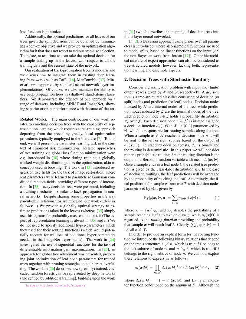
`4Figure 1. Each node n ∈ N of the tree performs routing decisionsvia function dn(·) (we omit the parametrization Θ). The blackpath shows an exemplary routing of a sample x along a tree toreach leaf `4, which has probability µ`4 = d1(x)d2(x)d5(x).

product in (2) runs over all nodes, only decision nodes alongthe path from the root node to the leaf ` contribute to µ`,because for all other nodes 1`↙n and 1n↘` will be both 0(assuming 00 = 1, see Fig. 1 for an illustration).

Decision nodes In the rest of the paper we consider deci-sion functions delivering a stochastic routing with decisionfunctions defined as follows:

dn(x; Θ) = σ(fn(x; Θ)) , (3)

where σ(x) = (1 + e−x)−1 is the sigmoid function, andfn(·; Θ) : X → R is a real-valued function dependingon the sample and the parametrization Θ. Further detailsabout the functions fn can be found in Section 4.1, but in-tuitively depending on how we choose these functions wecan model trees having shallow decisions (e.g. such as inoblique forests [13]) as well as deep ones.

Forests of decision trees. A forest is an ensemble of de-cision trees F = {T1, . . . , Tk}, which delivers a predictionfor a sample x by averaging the output of each tree, i.e.

PF [y|x] =1

k

k∑h=1

PTh[y|x] , (4)

omitting the tree parameters for notational convenience.

3. Learning Trees by Back-PropagationLearning a decision tree modeled as in Section 2 requires

estimating both, the decision node parametrizations Θ andthe leaf predictions π. For their estimation we adhere to theminimum empirical risk principle with respect to a givendata set T ⊂ X × Y under log-loss, i.e. we search for theminimizers of the following risk term:

R(Θ,π; T ) =1

|T |∑

(x,y)∈T

L(Θ,π;x, y) , (5)

where L(Θ,π;x, y) is the log-loss term for the trainingsample (x, y) ∈ T , which is given by

L(Θ,π;x, y) = − log(PT [y|x,Θ,π]) , (6)

and PT is defined as in (1).We consider a two-step optimization strategy, described

in the rest of this section, where we alternate updates of Θwith updates of π in a way to minimize (5).

3.1. Learning Decision Nodes

All decision functions depend on a common parameterΘ, which in turn parametrizes each function fn in (3). Sofar, we made no assumptions about the type of functions infn, therefore nothing prevents the optimization of the riskwith respect to Θ for a given π from eventually becominga difficult and large-scale optimization problem. As an ex-ample, Θ could absorb all the parameters of a deep neuralnetwork having fn as one of its output units. For this rea-son, we will employ a Stochastic Gradient Descent (SGD)approach to minimize the risk with respect to Θ, as com-monly done in the context of deep neural networks:

Θ(t+1) = Θ(t) − η ∂R∂Θ

(Θ(t),π;B)

= Θ(t) − η

|B|∑

(x,y)∈B

∂L

∂Θ(Θ(t),π;x, y)

(7)

Here, 0 < η is the learning rate and B ⊆ T is a randomsubset (a.k.a. mini-batch) of samples from the training set.Although not shown explicitly, we additionally consider amomentum term to smooth out the variations of the gradi-ents. The gradient of the loss L with respect to Θ can bedecomposed by the chain rule as follows

∂L

∂Θ(Θ,π;x, y) =

∑n∈N

∂L(Θ,π;x, y)

∂fn(x; Θ)

∂fn(x; Θ)

∂Θ. (8)

Here, the gradient term that depends on the decision tree isgiven by

∂L(Θ,π;x, y)

∂fn(x; Θ)= dn(x; Θ)Anr

− dn(x; Θ)Anl, (9)

where nl and nr indicate the left and right child of node n,respectively, and we define Am for a generic node m ∈ Nas

Am =

∑`∈Lm

π`yµ`(x|Θ)

PT [y|x,Θ,π].

With Lm ⊆ L we denote the set of leaves held by the sub-tree rooted in node m. Detailed derivations of (9) can befound in Section 2 of the supplementary document. More-over, in Section 4 we describe how Am can be efficientlycomputed for all nodes m with a single pass over the tree.

As a final remark, we considered also an alternativeoptimization procedure to SGD, namely Resilient Back-Propagation (RPROP) [27], which automatically adapts aspecific learning rate for each parameter based on the signchange of its risk partial derivative over the last iteration.

3.2. Learning Prediction Nodes

Given the update rules for the decision function parame-ters Θ from the previous subsection, we now consider theproblem of minimizing (5) with respect to π when Θ isfixed, i.e.

minπR(Θ,π; T ) . (10)

This is a convex optimization problem and a global solutioncan be easily recovered. A similar problem has been en-countered in the context of decision trees in [28], but onlyat the level of a single node. In our case, however, the wholetree is taken into account, and we are jointly estimating allthe leaf predictions.

In order to compute a global minimizer of (10) we pro-pose the following iterative scheme:

π(t+1)`y =

1

Z(t)`

∑(x,y′)∈T

1y=y′ π(t)`y µ`(x|Θ)

PT [y|x,Θ,π(t)], (11)

for all ` ∈ L and y ∈ Y , where Z(t)` is a normalizing fac-

tor ensuring that∑

y π(t+1)`y = 1. The starting point π(0)

can be arbitrary as long as every element is positive. Atypical choice is to start from the uniform distribution inall leaves, i.e. π(0)

`y = |Y|−1. It is interesting to note thatthe update rule in (11) is step-size free and it guarantees astrict decrease of the risk at each update until a fixed-pointis reached (see proof in supplementary material).

As opposed to the update strategy for Θ, which is basedon mini-batches, we adopt an offline learning approach toobtain a more reliable estimate of π, because suboptimalpredictions in the leaves have a strong impact on the finalprediction. Moreover, we interleave the update of π with awhole epoch of stochastic updates of Θ as described in theprevious subsection.

3.3. Learning a Forest

So far we have dealt with a single decision tree setting.Now, we consider an ensemble of trees F , where all treescan possibly share same parameters in Θ, but each tree canhave a different structure with a different set of decisionfunctions (still defined as in (3)), and independent leaf pre-dictions π.

Since each tree in forest F has its own set of leaf pa-rameters π, we can update the prediction nodes of each treeindependently as described in Subsection 3.2, given the cur-rent estimate of Θ.

As for Θ, instead, we randomly select a tree inF for eachmini-batch and then we proceed as detailed in Subsection3.1 for the SGD update. This strategy somewhat resemblesthe basic idea of Dropout [34], where each SGD update ispotentially applied to a different network topology, whichis sampled according to a specific distribution. In addition,updating individual trees instead of the entire forest reducesthe computational load during training.

During test time, as shown in (4), the prediction deliv-ered by each tree is averaged to produce the final outcome.

3.4. Summary of the Learning Procedure

The learning procedure is summarized in Algorithm 1.We start with a random initialization of the decision nodesparameters Θ and iterate the learning procedure for a pre-determined number of epochs, given a training set T . Ateach epoch, we initially obtain an estimation of the pre-diction node parameters π given the actual value of Θ byrunning the iterative scheme in (11), starting from the uni-form distribution in each leaf, i.e. π(0)

`y = |Y|−1. Then wesplit the training set into a random sequence of mini-batchesand we perform for each mini-batch a SGD update of Θ asin (7). After each epoch we might eventually change thelearning rate according to pre-determined schedules.

More details about the computation of some tree-specificterms are given in the next section.

Algorithm 1 Learning trees by back-propagationRequire: T : training set, nEpochs

1: random initialization of Θ2: for all i ∈ {1, . . . , nEpochs} do3: Compute π by iterating (11)4: break T into a set of random mini-batches5: for all B: mini-batch from T do6: Update Θ by SGD step in (7)7: end for8: end for

4. Implementation Notes4.1. Decision Nodes

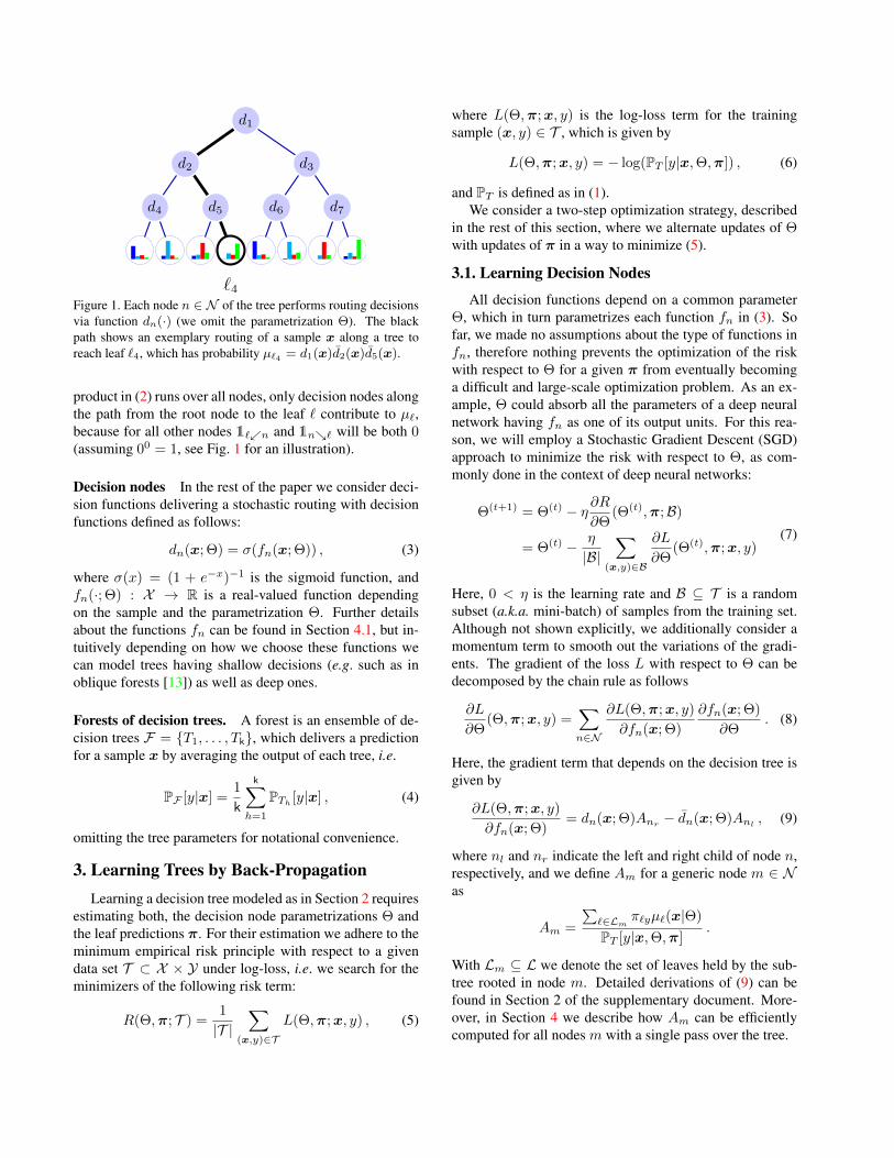
We have defined decision functions dn in terms of real-valued functions fn(·; Θ), which are not necessarily inde-pendent, but coupled through the shared parametrization Θ.Our intention is to endow the trees with feature learning ca-pabilities by embedding functions fn within a deep convo-lutional neural network with parameters Θ. In the specific,we can regard each function fn as a linear output unit of adeep network that will be turned into a probabilistic rout-ing decision by the action of dn, which applies a sigmoidactivation to obtain a response in the [0, 1] range. Fig. 2provides a schematic illustration of this idea, showing how

d1

d2

d4

π1 π2

d5

π3 π4

d3

d6

π5 π6

d7

π7 π8

f7f3f6f1f5f2f4

d8

d9

d11

π9 π10

d12

π11 π12

d10

d13

π13 π14

d14

π15 π16

f14f10f13f8f12f9f11FC

Deep CNN with parameters Θ

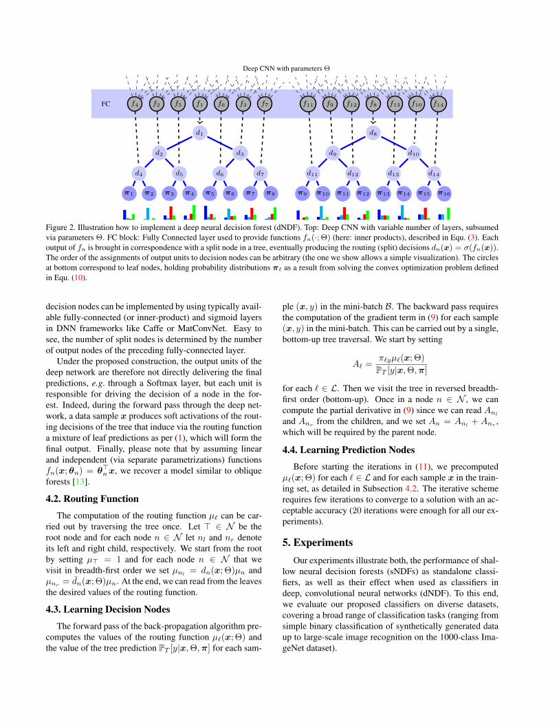
Figure 2. Illustration how to implement a deep neural decision forest (dNDF). Top: Deep CNN with variable number of layers, subsumedvia parameters Θ. FC block: Fully Connected layer used to provide functions fn(·; Θ) (here: inner products), described in Equ. (3). Eachoutput of fn is brought in correspondence with a split node in a tree, eventually producing the routing (split) decisions dn(x) = σ(fn(x)).The order of the assignments of output units to decision nodes can be arbitrary (the one we show allows a simple visualization). The circlesat bottom correspond to leaf nodes, holding probability distributions π` as a result from solving the convex optimization problem definedin Equ. (10).

decision nodes can be implemented by using typically avail-able fully-connected (or inner-product) and sigmoid layersin DNN frameworks like Caffe or MatConvNet. Easy tosee, the number of split nodes is determined by the numberof output nodes of the preceding fully-connected layer.

Under the proposed construction, the output units of thedeep network are therefore not directly delivering the finalpredictions, e.g. through a Softmax layer, but each unit isresponsible for driving the decision of a node in the for-est. Indeed, during the forward pass through the deep net-work, a data sample x produces soft activations of the rout-ing decisions of the tree that induce via the routing functiona mixture of leaf predictions as per (1), which will form thefinal output. Finally, please note that by assuming linearand independent (via separate parametrizations) functionsfn(x;θn) = θ>nx, we recover a model similar to obliqueforests [13].

4.2. Routing Function

The computation of the routing function µ` can be car-ried out by traversing the tree once. Let > ∈ N be theroot node and for each node n ∈ N let nl and nr denoteits left and right child, respectively. We start from the rootby setting µ> = 1 and for each node n ∈ N that wevisit in breadth-first order we set µnl

= dn(x; Θ)µn andµnr = dn(x; Θ)µn. At the end, we can read from the leavesthe desired values of the routing function.

4.3. Learning Decision Nodes

The forward pass of the back-propagation algorithm pre-computes the values of the routing function µ`(x; Θ) andthe value of the tree prediction PT [y|x,Θ,π] for each sam-

ple (x, y) in the mini-batch B. The backward pass requiresthe computation of the gradient term in (9) for each sample(x, y) in the mini-batch. This can be carried out by a single,bottom-up tree traversal. We start by setting

A` =π`yµ`(x; Θ)

PT [y|x,Θ,π]

for each ` ∈ L. Then we visit the tree in reversed breadth-first order (bottom-up). Once in a node n ∈ N , we cancompute the partial derivative in (9) since we can read Anl

and Anrfrom the children, and we set An = Anl

+ Anr,

which will be required by the parent node.

4.4. Learning Prediction Nodes

Before starting the iterations in (11), we precomputedµ`(x; Θ) for each ` ∈ L and for each sample x in the train-ing set, as detailed in Subsection 4.2. The iterative schemerequires few iterations to converge to a solution with an ac-ceptable accuracy (20 iterations were enough for all our ex-periments).

5. ExperimentsOur experiments illustrate both, the performance of shal-

low neural decision forests (sNDFs) as standalone classi-fiers, as well as their effect when used as classifiers indeep, convolutional neural networks (dNDF). To this end,we evaluate our proposed classifiers on diverse datasets,covering a broad range of classification tasks (ranging fromsimple binary classification of synthetically generated dataup to large-scale image recognition on the 1000-class Ima-geNet dataset).

G50c [33] Letter [10] USPS [14] MNIST [20] Char74k[8]

# Train Samples 50 16000 7291 60000 66707# Test Samples 500 4000 2007 10000 7400# Classes 2 26 10 10 62# Input dimensions 50 16 256 784 64

Alternating Decision Forest (ADF) [30] 18.71±1.27 3.52±0.17 5.59±0.16 2.71±0.10 16.67±0.21Shallow Neural Decision Forest (sNDF) 17.4±1.52 2.92±0.17 5.01±0.24 2.8±0.12 16.04±0.20

Tree input features 10 (random) 8 (random) 10x10 patches 15x15 patches 10 (random)Depth 5 10 10 10 12Number of trees 50 70 100 80 200Batch size 25 500 250 1000 1000

Table 1. Comparison of alternating decision forests (ADF) to shallow neural decision forests (sNDFs, no hidden layers) on selected standardmachine learning datasets. Top: Details about datasets. Middle: Average error [%] (with corresponding standard deviation) obtained from10 repetitions of the experiment. Bottom: Details about the parametrization of our model.

5.1. Comparison of sNDFs to Forest Classifiers

We first compared sNDFs against state-of-the-art interms of stand-alone, off-the-shelf forest ensembles. In or-der to have a fair comparison, our classifier is built withouthidden layers, i.e. we consider feature mappings having thesimple form fn(x;θn) = θ>nx. We used the 5 datasets in[30] to compare the performance of sNDFs to that of Alter-nating Decision Forests (ADF). The details of this experi-ment are summarized in Tab. 1. For ADF, we provide re-sults reported in their paper and we use their reported max-imal tree depth and forest size as an upper bound on thesize of our models. Essentially, for each of the datasets,all our trees are less deep and there are fewer of themthan in the corresponding ADF models. We used ensem-bles of different sizes depending on the size of the datasetand the complexity of the learning tasks. In all cases, weuse RPROP and the recommended hyper-parameters of theoriginal publication [27] for split node parameter optimiza-tion. We report the average error with standard deviationsresulting from 10 repetitions of the experiment. Overall, weoutperform ADF, though significant results, with p-valuesless than 0.05, were obtained for the Letter, USPS andChar74k datasets.

5.2. Improving Performance with dNDF

In the following experiments we integrated our novel for-est classifiers in end-to-end image classification pipelines,using multiple convolutional layers for representation learn-ing as typically done in deep learning systems.

5.2.1 MNIST

We used the MatConvNet library [37] and their referenceimplementation of LeNet-5 [21], for building an end-to-enddigit classification system on MNIST training data, replac-ing the conventionally used Softmax layer by our forest.

The baseline yields an error of 0.9% on test data, which weobtained by re-running the provided example architecturewith given settings for optimization, hyper-parameters, etc.By using our proposed dNDF on top of LeNet-5, each deci-sion function being driven by an output unit fully connectedto the last hidden layer of the CNN, we can reduce the clas-sification error to 0.7%. The ensemble size was fixed to 10trees, each with a depth of 5. Please note the positive ef-fect on MNIST performance compared to Section 5.1 whenspending additional layers on representation learning.

5.2.2 ImageNet

ImageNet [29] is a benchmark for large-scale image recog-nition tasks and its images are assigned to a single outof 1000 possible ground truth labels. The dataset con-tains ≈1.2M training images, 50.000 validation imagesand 100.000 test images with average dimensionality of482x415 pixels. Training and validation data are pub-licly available and we followed the commonly agreed pro-tocol by reporting Top5-Errors on validation data. TheGoogLeNet architecture [36], which has a reported Top5-Error of 10.07% when used in a single-model, single-cropsetting (see first row in Tab. 3 in [36]) served as basis forour experiments. It uses 3 Softmax layers at different stagesof the network to encourage the construction of informativefeatures, due to its very deep architecture. Each of theseSoftmax layers gets their input from a Fully Connected (FC)layer, built on top of an Average Pool layer, which in turn isbuilt on top of a corresponding Concat layer. Let DC0, DC1and DC2 be the Concat layers preceding each of the Soft-max layers in GoogLeNet. Let AvgPool0, AvgPool1 andAvgPool2 be the Average Pool layers preceding these Soft-max layers. To avoid problems with propagation of gradi-ents given the depth of the network and in order to providethe final classification layers with the features obtained inthe early stages of the pipeline, we have also supplied DC0

GoogLeNet [36] GoogLeNet? dNDF.NET

# Models 1 7 1 1 7# Crops 1 10 144 1 10 144 1 1 10 1

Top5-Errors 10.07% 9.15% 7.89% 8.09% 7.62% 6.67% 10.02% 7.84% 7.08% 6.38%Table 2. Top5-Errors obtained on ImageNet validation data, comparing our dNDF.NET to GoogLeNet(?).

as input to AvgPool1 and AvgPool2 and DC1 as input toAvgPool2. We have implemented this modified networkusing the Distributed (Deep) Machine Learning Common(DMLC) library [22]2 and dub it GoogLeNet?. Its single-model, single crop Top5-Error is 10.02% (when trainedwith SGD, 0.9 momentum, fixed learning rate schedule, de-creasing the learning rate by 4% every 8 epochs and mini-batches composed of 50 images).

In order to obtain a Deep Neural Decision Forest ar-chitecture coined dNDF.NET, we have replaced each Soft-max layer from GoogLeNet? with a forest consisting of 10trees (each fixed to depth 15), resulting in a total numberof 30 trees. We refer to the individual forests as dNDF0

(closest to raw input), dNDF1 (replacing middle loss layerin GoogLeNet?) and dNDF2 (as terminal layer). We pro-vide a visualization for our dNDF.NET architecture in thesupplementary document. Following the implementationguideline in Subsection 4.1, we randomly selected 500output dimensions of the respectively preceding layers inGoogLeNet? for each decision function fn. In such a way,a single FC layer with #trees × #split nodes/tree outputunits provides all the split node inputs per dNDFx. Theresulting architecture was implemented in DMLC as well,and we trained the network for 1000 epochs using (mini-)batches composed of 100.000 images (which was feasibledue to distribution of the computational load to a cluster of52 CPUs and 12 hosts, where each host is equipped with aNVIDIA Tesla K40 GPU).

For posterior learning, we only update the leaf node pre-dictions of the tree that also receives split node parameterupdates, i.e. the randomly selected one as described in Sub-section 3.3. To improve computational efficiency, we con-sider only the samples of the current mini-batch for pos-terior learning, while all the training data could be used inprinciple. However, since we use mini-batches composed of100.000 samples, we can approximate the training set suf-ficiently well while simultaneously introducing a positive,regularizing effect.

Tab. 2 provides a summary of Top5-Errors on valida-tion data for our proposed dNDF.NET against GoogLeNetand GoogLeNet?. We ascribe the improvements on the sin-gle crop, single model setting (Top5-Error of only 7.84%)to our proposed approach, as the only architectural differ-ence to GoogLeNet? (Top5-Error of 10.02%) is deploying

2https://github.com/dmlc/cxxnet.git

our dNDFs. By using an ensemble of 7 dNDF.NETs (stillsingle crop inputs), we can improve further and obtain aTop5-Error of 6.38%, which is better than the best result of6.67%, obtained with 7 GoogLeNets using 144 crops perimage [36]. Next, we discuss some operational characteris-tics of our single-model, single-crop setting.

Evaluation of tree nodes Intuitively, a tree-structuredclassifier aims to produce pure leaf node distributions. Thismeans that the training error is reduced by (repeatedly) par-titioning the input space in a way such that it correlates withtarget classes in Y .

Analyzing the outputs of decision functions fn is infor-mative about the routing uncertainties for a given sample x,as it traverses the tree(s). In Fig. 3, we show histogramsof all available split node outputs of our three forests (i.e.dNDF0, dNDF1, dNDF2) for all samples of the validationset after running for 100, 500 and 1000 epochs over thetraining data. The leftmost histogram (after 100 trainingepochs) shows the highest uncertainty about the routing di-rection, i.e. the split decisions are not yet very crisp suchthat a sample will be routed to many leaf nodes. As train-ing progresses (middle and right plots after 500 and 1000epochs), we can see how the distributions get very peakedat 0 and 1 (i.e. samples are routed either to the left or rightchild with low uncertainty), respectively. As a result, thesamples will only be routed to a small subset of availableleaf nodes with reasonably high probability. In other words,most available leaves will never be reached from a sample-centric view and therefore only a small number of overallpaths needs to be evaluated at test time. As part of futurework and in order to decrease computational load, we planto route samples along the trees by sampling from these splitdistributions, rather than sending them to every leaf node.

To assess the quality of the resulting leaf posterior dis-tributions obtained from the global optimization procedure,we illustrate how the mean leaf entropy develops as a func-tion of training epochs (see Fig. 4). To this end, we ran-domly selected 1024 leaves from all available ones per treeand computed their mean entropy after each epoch. Thehighest entropy would result from a uniform distributionand is ≈9.96 bits for a 1000-class problem. Instead, wewant to obtain highly peaked distributions for the leaf pre-dictors, leading to low entropy. Indeed, the average entropydecreases as training progresses, confirming the efficacy ofour proposed leaf node parameter learning approach.

Split node output0 0.1 0.2 0.3 0.4 0.5 0.6 0.7 0.8 0.9 1

His

togr

am c

ount

s

#108

0

1

2

3

4

5

6

7Split responses on validation set (100 training epochs)

Split node output0 0.1 0.2 0.3 0.4 0.5 0.6 0.7 0.8 0.9 1

His

togr

am c

ount

s

#108

0

2

4

6

8

10

12Split responses on validation set (500 training epochs)

Split node output0 0.1 0.2 0.3 0.4 0.5 0.6 0.7 0.8 0.9 1

His

togr

am c

ount

s

#109

0

0.5

1

1.5

2

2.5Split responses on validation set (1k training epochs)

Figure 3. Histograms over all split node responses of all three forests in dNDF.NET on ImageNet validation data after accomplishing100 (left), 500 (middle) and 1000 (right) epochs over training data. As training progresses, the split node outputs approach 0 or 1 whichcorresponds to eliminating routing uncertainty of samples when being propagated through the trees.

100 200 300 400 500 600 700 800 900 10003

4

5

6

7

8

9

# Training Epochs

Avera

ge L

eaf E

ntr

opy [bits]

Average Leaf Entropy during Training

Figure 4. Average leaf entropy development as a function of train-ing epochs in dNDF.NET.

Evaluation of model performance In Fig. 5 we showthe development of Top5-Errors for each dNDFx indNDF.NET as well as their ensemble performances as afunction of training epochs. The left plot shows the devel-opment over all training epochs (1000 in total) while theright plot is a zoomed view from epochs 500 to 1000 andTop5-Errors 0–12%. As expected, dNDF0 (which is clos-est to the input layer) performs worse than dNDF2, whichconstitutes the final layer of dNDF.NET, however, onlyby 1.34%. Consequently, the computational load betweendNDF0 and dNDF2 could be traded for a degradation ofonly 1.34% in accuracy during inference. Conversely, tak-ing the mean over all three dNDFs yields the lowest Top5-Error of 7.84% after 1000 epochs over training data.

6. Conclusions

In this paper we have shown how to model and trainstochastic, differentiable decision trees, usable as alterna-tive classifiers for end-to-end learning in (deep) convolu-tional networks. Prevailing approaches for decision treetraining typically operate in a greedy and local manner,

#Training Epochs0 200 400 600 800 1000

Top

5-E

rror

[%]

0

20

40

60

80

100

#Training Epochs500 550 600 650 700 750 800 850 900 950 1000

Top

5-E

rror

[%]

00.5

11.5

22.5

33.5

44.5

55.5

66.5

77.5

88.5

99.510

10.511

11.512

ImageNet Top5-Errors

dNDF0 on Validation

dNDF1 on Validation

dNDF2 on Validation

dNDF.NET on ValidationdNDF.NET on Training

Figure 5. Top5-Error plots for individual dNDFx used indNDF.NET as well as their joint ensemble errors. Left: Plot overall 1000 training epochs. Right: Zoomed version of left plot,showing Top5-Errors from 0–12% between training epochs 500-1000.

making representation learning impossible. To overcomethis problem, we introduced stochastic routing for deci-sion trees, enabling split node parameter learning via back-propagation. Moreover, we showed how to populate leafnodes with their optimal predictors, given the current stateof the tree/underlying network. We have successfully vali-dated our new decision forest model as stand-alone classi-fier on standard machine learning datasets and surpass state-of-the-art performance on ImageNet when integrating themin the GoogLeNet architecture, without any form of datasetaugmentation.

Acknowledgments Peter and Samuel were partially sup-ported by Novartis Pharmaceuticals and the ASSESS MSproject. Madalina was partially supported by the NationalScience Foundation under Award 1320347 and by the De-fense Advanced Research Projects Agency under ContractFA8750-12-2-0324. We thank Alex Smola and Mu Li forgranting us access to run ImageNet experiments on theirserver infrastructure and Darko Zikic for fruitful discus-sions.

References[1] Y. Amit and D. Geman. Shape quantization and recognition

with randomized trees. (NC), 9(7):1545–1588, 1997. 1[2] C. M. Bishop and M. Svensen. Bayesian hierarchical mix-

tures of experts. In Proc. of Conference on Uncertainty inArtificial Intelligence, pages 57–64, 2003. 2

[3] A. Bosch, A. Zisserman, and X. Munoz. Image classificationusing random forests and ferns. In (ICCV), 2007. 1

[4] L. Breiman. Random forests. Machine Learning, 45(1):5–32, 2001. 1

[5] G. J. Brostow, J. Shotton, J. Fauqueur, and R. Cipolla. Seg-mentation and recognition using structure from motion pointclouds. In (ECCV). Springer, 2008. 1

[6] R. Caruana, N. Karampatziakis, and A. Yessenalina. An em-pirical evaluation of supervised learning in high dimensions.In (ICML), pages 96–103, 2008. 1

[7] A. Criminisi and J. Shotton. Decision Forests in ComputerVision and Medical Image Analysis. Springer, 2013. 1, 2

[8] T. E. de Campos, B. R. Babu, and M. Varma. Characterrecognition in natural images. In Proceedings of the Interna-tional Conference on Computer Vision Theory and Applica-tions, Lisbon, Portugal, February 2009. 6

[9] A. K. L. Fei-Fei. Deep visual-semantic alignments for gen-erating image descriptions. In (CVPR), 2015. 1

[10] P. W. Frey and D. J. Slate. Letter recognition using holland-style adaptive classifiers. (ML), 6(2), Mar. 1991. 6

[11] T. Hastie, R. Tibshirani, and J. H. Friedman. The Elementsof Statistical Learning. Springer, 2009. 1

[12] K. He, X. Zhang, S. Ren, and J. Sun. Delving deep intorectifiers: Surpassing human-level performance on imagenetclassification. CoRR, abs/1502.01852, 2015. 1

[13] D. Heath, S. Kasif, and S. Salzberg. Induction of obliquedecision trees. Journal of Artificial Intelligence Research,2(2):1–32, 1993. 3, 5

[14] J. J. Hull. A database for handwritten text recognition re-search. (PAMI), 16(5):550–554, 1994. 6

[15] J. Jancsary, S. Nowozin, and C. Rother. Loss-specific train-ing of non-parametric image restoration models: A new stateof the art. In (ECCV), 2012. 2

[16] Y. Jia, E. Shelhamer, J. Donahue, S. Karayev, J. Long, R. Gir-shick, S. Guadarrama, and T. Darrell. Caffe: Convolu-tional architecture for fast feature embedding. arXiv preprintarXiv:1408.5093, 2014. 2

[17] M. I. Jordan. Hierarchical mixtures of experts and the emalgorithm. (NC), 6:181–214, 1994. 2

[18] P. Kontschieder, P. Kohli, J. Shotton, and A. Criminisi. GeoF:Geodesic forests for learning coupled predictors. In (CVPR),pages 65–72, 2013. 1

[19] A. Krizhevsky, I. Sutskever, and G. Hinton. Imagenet classi-fication with deep convolutional neural networks. In (NIPS),2012. 1

[20] Y. Lecun, L. Bottou, Y. Bengio, and P. Haffner. Gradient-based learning applied to document recognition. In Proceed-ings of the IEEE, pages 2278–2324, 1998. 6

[21] Y. LeCun, L. Bottou, G. Orr, and K. Muller. Efficient back-prop. In G. Orr and M. K., editors, Neural Networks: Tricksof the trade. Springer, 1998. 6

[22] M. Li, D. G. Andersen, J. W. Park, A. J. Smola, A. Ahmed,V. Josifovski, J. Long, E. J. Shekita, and B.-Y. Su. Scalingdistributed machine learning with the parameter server. In11th USENIX Symposium on Operating Systems Design andImplementation (OSDI 14). USENIX Association, 2014. 7

[23] M. Lin, Q. Chen, and S. Yan. Network in network. CoRR,abs/1312.4400, 2013. 1

[24] A. Montillo, J. Tu, J. Shotton, J. Winn, J. E. Iglesias, D. N.Metaxas, and A. Criminisi. Entangled forests and differen-tiable information gain maximization. In Decision Forestsin Computer Vision and Medical Image Analysis. Springer,2013. 1, 2

[25] S. Ren, X. Cao, Y. Wei, and J. Sun. Global refinement ofrandom forest. In (CVPR), 2015. 2

[26] D. L. Richmond, D. Kainmueller, M. Y. Yang, E. W. My-ers, and C. Rother. Relating cascaded random forests todeep convolutional neural networks for semantic segmenta-tion. CoRR, abs/1507.07583, 2015. 2

[27] M. Riedmiller and H. Braun. A direct adaptive method forfaster backpropagation learning: The RPROP algorithm. InIEEE Conf. on Neural Networks, 1993. 4, 6

[28] S. Rota Bulo and P. Kontschieder. Neural decision forests forsemantic image labelling. In (CVPR), 2014. 1, 4

[29] O. Russakovsky, J. Deng, H. Su, J. Krause, S. Satheesh,S. Ma, Z. Huang, A. Karpathy, A. Khosla, M. Bernstein,A. C. Berg, and L. Fei-Fei. ImageNet Large Scale VisualRecognition Challenge. International Journal of ComputerVision (IJCV), 2014. 6

[30] S. Schulter, P. Wohlhart, C. Leistner, A. Saffari, P. M. Roth,and H. Bischof. Alternating decision forests. In (CVPR),2013. 2, 6

[31] I. Sethi. Entropy nets: from decision trees to neural net-works. Proceedings of the IEEE, 78(10), 1990. 2

[32] J. Shotton, R. Girshick, A. Fitzgibbon, T. Sharp, M. Cook,M. Finocchio, R. Moore, P. Kohli, A. Criminisi, A. Kipman,and A. Blake. Efficient human pose estimation from singledepth images. (PAMI), 2013. 1

[33] V. Sindhwani, P. Niyogi, and M. Belkin. Beyond the pointcloud: From transductive to semi-supervised learning. In(ICML), pages 824–831. ACM, 2005. 6

[34] N. Srivastava, G. Hinton, A. Krizhevsky, I. Sutskever, andR. Salakhutdinov. Dropout: A simple way to prevent neu-ral networks from overfitting. Journal of Machine LearningResearch, 15:1929–1958, 2014. 4

[35] A. Suarez and J. F. Lutsko. Globally optimal fuzzy decisiontrees for classification and regression. (PAMI), 21(12):1297–1311, 1999. 2

[36] C. Szegedy, W. Liu, Y. Jia, P. Sermanet, S. Reed,D. Anguelov, D. Erhan, V. Vanhoucke, and A. Rabinovich.Going deeper with convolutions. CoRR, abs/1409.4842,2014. 1, 6, 7

[37] A. Vedaldi and K. Lenc. Matconvnet – convolutional neuralnetworks for matlab. CoRR, abs/1412.4564, 2014. 2, 6

[38] D. Yu and L. Deng. Automatic Speech Recognition: A DeepLearning Approach. Springer, 2014. 1