Rochester Institute of TechnologyRIT Scholar Works

Theses Thesis/Dissertation Collections

2012

Deep learning using genetic algorithmsJoshua Lamos-Sweeney

Follow this and additional works at: http://scholarworks.rit.edu/theses

This Thesis is brought to you for free and open access by the Thesis/Dissertation Collections at RIT Scholar Works. It has been accepted for inclusionin Theses by an authorized administrator of RIT Scholar Works. For more information, please contact ritscholarworks@rit.edu.

Recommended CitationLamos-Sweeney, Joshua, "Deep learning using genetic algorithms" (2012). Thesis. Rochester Institute of Technology. Accessed from

Deep Learning Using Genetic Algorithms

Joshua D. Lamos-Sweeney

May 17, 2012

A Thesis Submitted in Partial Fulfillment of the Requirements for theDegree of Master of Computer Science

Department of Computer ScienceB. Thomas Golisano College of Computing and Information Sciences

Rochester Institute of TechnologyRochester, NY

AdvisorDr. Roger Gaborski

ReaderDr. Peter Anderson

ObserverYuheng Wang

i

Contents

1 Introduction 11.1 Deep Learning . . . . . . . . . . . . . . . . . . . . . . . . . . 21.2 Genetic Algorithms . . . . . . . . . . . . . . . . . . . . . . . . 4

2 Uses of a Trained Network 52.1 Classification . . . . . . . . . . . . . . . . . . . . . . . . . . . 52.2 Search . . . . . . . . . . . . . . . . . . . . . . . . . . . . . . . 62.3 Data Reduction . . . . . . . . . . . . . . . . . . . . . . . . . . 72.4 Data Mining . . . . . . . . . . . . . . . . . . . . . . . . . . . 8

3 Network Implementation 93.1 Basic Network Design . . . . . . . . . . . . . . . . . . . . . . 93.2 Genetics and Network Design . . . . . . . . . . . . . . . . . . 113.3 Sparse Network Design . . . . . . . . . . . . . . . . . . . . . . 13

4 Results 164.1 Parameters . . . . . . . . . . . . . . . . . . . . . . . . . . . . 16

4.1.1 Mutation . . . . . . . . . . . . . . . . . . . . . . . . . 164.1.2 Elitism . . . . . . . . . . . . . . . . . . . . . . . . . . 164.1.3 Enforced Sparseness . . . . . . . . . . . . . . . . . . . 174.1.4 Multithreading . . . . . . . . . . . . . . . . . . . . . . 174.1.5 Selection Method . . . . . . . . . . . . . . . . . . . . . 174.1.6 Layers . . . . . . . . . . . . . . . . . . . . . . . . . . . 19

4.2 Handwriting . . . . . . . . . . . . . . . . . . . . . . . . . . . . 194.3 Face Images . . . . . . . . . . . . . . . . . . . . . . . . . . . . 194.4 Cat Images . . . . . . . . . . . . . . . . . . . . . . . . . . . . 214.5 Large Faces . . . . . . . . . . . . . . . . . . . . . . . . . . . . 234.6 Missing Data Tests . . . . . . . . . . . . . . . . . . . . . . . . 23

5 Entropy 25

6 Future Work 25

ii

Abstract

Deep Learning networks are a new type of neural network that dis-covers important object features. These networks determine featureswithout supervision, and are adept at learning high level abstractionsabout their data sets.

These networks are useful for a variety of tasks, but are difficultto train. This difficulty is compounded when multiple networks aretrained in a layered fashion, which results in increased solution com-plexity as well as increased training time.

This paper examines the use of Genetic Algorithms as a trainingmechanism for Deep Learning networks, with emphasis on trainingnetworks with a large number of layers, each of which is trained inde-pendently to reduce the computational burden and increase the overallflexibility of the algorithm.

This paper covers the implementation of a multilayer deep learn-ing network using a genetic algorithm, including tuning the geneticalgorithm, as well as results of experiments involving data compres-sion and object classification. This paper aims to show that a geneticalgorithm can be used to train a non trivial deep learning network inplace of existing methodologies for network training, and that the fea-tures extracted can be used for a variety of real world computationalproblems.

1 Introduction

The creation and training of deep learning networks requires significant com-

putation. This effectively limits the complexity of the networks to be trained.

Current solutions for training deep networks are time intensive and limited

in the supported neural network architectures[3]. By utilizing a different

training method, this paper proposes that more complicated network de-

signs can be attained.

Machine learning is an important field of computing dealing with the

acquisition of knowledge. In basic terms, learning is the process of infer-

ring structure in data. Learning is a complex task, which involves making

inferences based on a set of data. One major area of research into machine

learning involves the creation of feed forward neural networks. Neural net-

works are conglomerations of small logic units, each of which replicates a

simple mathematical function. Feed-forward networks rely on the concept

1

of layers, where all neurons in a layer only output to the next layer. This

allows all the data to have a specific, non-infinite chain from input to out-

put. Various methods exist to train these networks to produce a specific

output for any specific input. One of the common training methods, known

as error propagation, relies on adjusting the network based on how much

each neuron contributed to an error, with each neuron passing a part of its

error to each neuron which gave it input. By training these networks on a

set of data for which the correct output is known, the network will return

the appropriate results for similar data.

The first downside of these networks is that they need explicit output

design for each category of object to be studied. They also need large

data sets to work with, to classify all the differences that can occur. These

networks are limited by the simplicity of their network design. Each layer

can only perform a simple subset of all possible classifiers, relying on the

number of layers to increase the complexity of their classification functions.

However, adding layers scales the training time using conventional training

algorithms super-linearly. Thus, large, multilayer neural networks cannot

be trained in reasonable time. Once trained, the networks are relatively

rigid, being able to be applied only to the exact problem domain they are

trained against. A network designed to identify three different species of cat

in images, for instance, could not be used to find if an image did not contain

a cat. A new network, trained on images with and without cats, would have

to be constructed.

1.1 Deep Learning

In the simple networks described above, the important information to be

learned about the image was given ahead of time. The notations of how

each instance of an idea was to be classified was encoded as a set of ex-

pected outputs. Labelling the importance of these outputs, and choosing

meaningful differences to look for requires human intervention. Features

also build on each other. For example, the presence of eyes in an image is

a good indicator that there is a person in the image. One of the key points

2

of deep learning networks is the discovery of features by the algorithm[5].

By discovering relationships in the data set, features can be found more ac-

curately, and by increasing the complexity of the network by adding layers,

higher level features, or features concerned less with the structure, and more

with the content of the data, can be extracted from the data.

Deep Learning networks extract features by finding common elements

in data. By grouping these elements together, a relationship between the

elements becomes known. This, in turn, can be connected to another higher

level feature. For example, two pixels may always be of similar intensity.

These pixels are put together into a feature. As a group of these pixels

can share most of their data, one variable can represent the approximate

intensity of the group of pixels. If those images were of a face, these pixels

might be an eyelid being open or closed. Because of this grouping of low

level features, the intensity of the low level pixels, a higher level feature,

eyes opened, has been discovered.

Deep Learning networks are currently trained by an algorithm known

as Contrastive Divergence. Contrastive Divergence works under the basic

principles of conforming the outputs of the network to mimic the training

data. By estimating the distance between the current network and an opti-

mum training set, successively closer approximations of a trained algorithm

emerge[9]. However, estimating this function requires taking an estimate of

the total state of the network. As the network grows more complex, not only

does it take longer to train, but each training step increases in computation,

limiting the complexity of the networks.

As there is no specified output states, these networks can develop their

own rules, requiring less supervision during the learning process than feed

forward neural networks. And once trained, these networks can be used

more organically, being able to be used on many sub-areas of a problem,

including feature extraction, classification, and search.

3

1.2 Genetic Algorithms

Genetic Algorithms are a type of heuristic search algorithm, based on the

concepts of natural selection. The basic operation of a genetic algorithm is

simple. A population is created, usually through a random process. The

algorithm then runs in a series of steps, known as epochs. Each epoch,

new individuals are added to the population, and the worst members of the

population are removed. These cycles of survival mimic natural evolution.

There are many variations on Genetic Algorithms, and each one has its

own particular lexicon of terms and procedures[4]. This particular algorithm

utilizes a constant population, and iterates over a series of generations. In-

dividuals are created using mutation, where a single existing member of the

population is subtly changed, and crossover, where two individuals are com-

bined together to create a new individual. Individuals are removed through

a selection process, based on the correctness of their solution, known as their

fitness.

As a search technique, Genetic Algorithms are heuristics[10]. Heuristics

are optimization techniques which are not guaranteed to produce better re-

sults than the search methodology they rely on, in this case an exhaustive

search, but commonly outperform naive search methods. Heuristics employ

assumptions on the structure of the underlying data to attempt to short cut

the underlying search methods they are based on. Genetic Algorithms pos-

tulate that the search space contains gradients between poor solutions and

good solutions. Using this preconception, a Genetic Algorithm can search

through the data space focusing on better solutions. If the data followed

an ever decreasing error toward a single solution, it would be easy enough

to just follow the slope of the decrease towards the optimal value, but even

without discontinuities, or locations where the fitness follows unexpected

patterns, a simple algorithm can be fooled by local minima.

Because of this, Genetic Algorithms work best on solutions with few

discontinuities, but can deal with local minima and other difficulties seen

in sub-optimal search problems. The movement of a Genetic Algorithm

through a search space can be generalized into two basic motivations, explo-

4

ration and exploitation. Exploration covers the search space evenly, reducing

the chances that the algorithm will stay at a local minima, while exploita-

tion moves the algorithm towards better solutions. With well chosen explo-

ration, the algorithm can be shown to eventually try all possibilities, while

well chosen exploitation increases the speed in which the algorithm finds a

good solution.

Comparing Genetic Algorithms to the other ways to generate network

topologies, there are many advantages to be had[4, 7]. Genetic Algorithms

can be trained continuously until a certain condition is made, giving closer

approximations to a correct solution. As a search heuristic, a GA will eventu-

ally try all combinations. Genetic Algorithms are a good fit for the problem

at hand, as there are no discontinuities, but many different good solutions.

Genetically created Deep learning networks can be easily layered, with

each layer working on the output of the previous layer, reducing the number

of features stored in an image. These networks can be trained sequentially;

each network is considered fixed by all networks after it. Using this learning

strategy, multi layer networks can scale linearly, as each network can be

trained independently.

2 Uses of a Trained Network

2.1 Classification

Once a network is trained against a subset of valid objects, one of the tasks

that the network can be used for is classification. In the simplest form, a

classification problem can be stated as such: given an object and a set, is

this object in the set. One of the underlying principles of the deep learning

architecture is the reconstruction of valid objects into their original pattern.

Of course, if a random image is sent into such a network, it will not resemble

itself very well. However, if the object is a close relation to the objects

trained, it should be reconstructed with a high fidelity. Using this, a simple

threshold can be established, and if the reconstruction is in error beyond

this threshold, it can be declared not in the set.

5

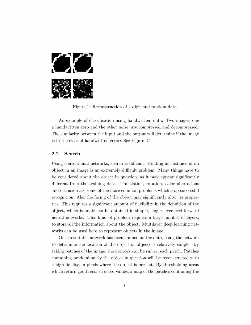
Figure 1: Reconstruction of a digit and random data.

An example of classification using handwritten data. Two images, one

a handwritten zero and the other noise, are compressed and decompressed.

The similarity between the input and the output will determine if the image

is in the class of handwritten zeroes See Figure 2.1.

2.2 Search

Using conventional networks, search is difficult. Finding an instance of an

object in an image is an extremely difficult problem. Many things have to

be considered about the object in question, as it may appear significantly

different from the training data. Translation, rotation, color aberrations

and occlusion are some of the more common problems which stop successful

recognition. Also the facing of the object may significantly alter its proper-

ties. This requires a significant amount of flexibility in the definition of the

object, which is unable to be obtained in simple, single layer feed forward

neural networks. This kind of problem requires a large number of layers,

to store all the information about the object. Multilayer deep learning net-

works can be used here to represent objects in the image.

Once a suitable network has been trained on the data, using the network

to determine the location of the object or objects is relatively simple. By

taking patches of the image, the network can be run on each patch. Patches

containing predominantly the object in question will be reconstructed with

a high fidelity, in pixels where the object is present. By thresholding areas

which return good reconstructed values, a map of the patches containing the

6

object can be created. The intersection of these patches, naturally, contains

the object to be found.

This algorithm is written for image based search, as this paper is focused

on image manipulation; However there is no reason for similar techniques

cannot be used on other types of data.

2.3 Data Reduction

Deep Learning networks can recreate close approximations of their original

objects from a compressed form. Ignoring the cost of the network itself,

which is a substantial single cost, this algorithm will perform compression

on any object given to it.

If one assumes a perfectly trained matrix, such that each output is recre-

ated as perfectly as possible, it is easy to derive that the algorithm should

perform nearly to the optimal level of entropy, as stated in Shannon’s The-

orem. If there is only one object, it will be perfectly recreated using no

data, as the algorithm can simply record all of the data in the bias term.

If there are two objects, the two algorithm needs two non-zero rows, which

requires one bit of data to store. It can, if perfectly trained, save a 0 in

the case for the first object, and a 1 in the case of the second. The bias

row contains the first object, while the one reverse row contains the second

object minus the first object. Thus reconstruction is perfect. Pushing the

limits past Shannon’s theorem in this thought experiment cleanly goes to a

lossy approximation, where the optimal result is the median point between

the two objects, thus both objects have lost half their data. If each training

exemplar is given equal weight during training, and all the data to be stored

is perfectly trained in the algorithm, the result must be that each is given an

equal percentage of the entropy needed to create a perfect reconstruction.

Whether this training set can be achieved can be tested while training the

network. Choosing a minimal value, v, where v is the ceiling of the entropy

of the testing set, as the number of values in the intermediate state given

a perfectly trained matrix, will result in the recreation of all testing data

perfectly, with a storage cost per training entity equal to the ceiling of the

7

theoretical minimum amount of data which needs to be stored.

Choosing a minimal value, η, where η is the ceiling of the entropy of the

testing set of size θ, as the number of values, or in this case, as the value is a

double precision value capped at −1 to 1. Given a perfectly trained matrix

of size κ, the size of the data in the testing set, by η, it can restore each

input from a storage size of η with no loss of precision, with a total storage

cost of (κ × η) + (η × θ). Thus, given a properly trained network, a deep

learning network can become a near perfect algorithm for lossless file size

reduction, having only κ×η overhead over the theoretical minimum storage

requirement.

2.4 Data Mining

A deep learning network is designed to create a feature subset of the original

object. As training a deep learning network relies on keeping the maximal

amount of information about the differences in the patterns of objects in

these categories, it can be assumed that the internal representation of the

objects keeps as much of the variance between the objects as possible. Thus,

this form contains all the variance needed to perform tasks related to the

sorting of these objects, such as primary component analysis, and data min-

ing techniques. These patterns have significantly less dimensionality than

the input images, allowing for faster, more accurate partitioning of the data

space.

Modern Data Mining algorithms use simple dimensionality reduction

tools to reduce the size of the data space to be searched while maximizing

the distance between points. By reducing the amount of data to compare,

these algorithms reduce the run time of comparisons, and reduce confusion,

leading to better solutions. By automatically extracting features which are

important to recreating the image, a Deep Learning network can perform

much the same task, reducing the overall dimensionality of the data, without

reducing the importance of the data to the classification of the image.

8

3 Network Implementation

The deep learning networks created to test these theories can be represented

as matrices. Each matrix contains one row for each input, plus a bias row,

and one column for each output, plus a bias column. Encoding of data is

performed by a simple matrix multiplication, while decoding the data back

into the reconstructed input is performed by multiplying the output of the

first transformation by the matrix transpose of the input matrix. Both these

operations are scaled such that the resulting matrices are in the range of zero

to one, though no such limitation is applied to the transformation matrix.

3.1 Basic Network Design

The basic architecture of the networks is a Restricted Boltzmann Machine.

An RBM is a network where every neuron in a layer is connected to every

neuron in the next successive layer. No other connections are allowed. A

neural network in this configuration can be easily represented as a matrix,

where rows are the input neurons, and columns are the output neurons.

Values in this representation are the weights assigned to the connections.

By themselves, layers in an RBM are not very powerful. However, by

increasing the number of layers, complex logic can be represented by the

series of operations[3]. Training all the layers simultaneously is infeasible,

but if these layers are frozen once computed, the computation time required

to compute each layer becomes linear with respect to the number of layers.

If each layer is treated as the final layer, reducing the input into a smaller

number of features, it can be trained directly on the input. Once it has

frozen, its output can be considered the input for the next layer. Once these

nested layers have been trained, calculating the final feature set, as well as

the reconstructed input, requires applying each matrix in turn, as can be

seen in Figure 2. A simple example of a conversion can be seen in Table 1.

9

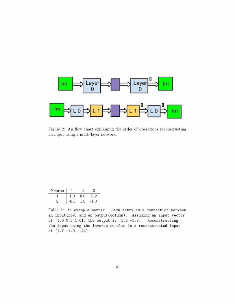
Figure 2: An flow chart explaining the order of operations reconstructingan input using a multi-layer network.

Neuron 1 2 3

1 1.0 0.0 0.22 -0.5 1.0 -1.0

Table 1: An example matrix. Each entry is a connection between

an input(row) and an output(column). Assuming an input vector

of [1.0 0.5 1.0], the output is [1.2 -1.0]. Reconstructing

the input using the inverse results in a reconstructed input

of [1.7 -1.0 1.24].

10

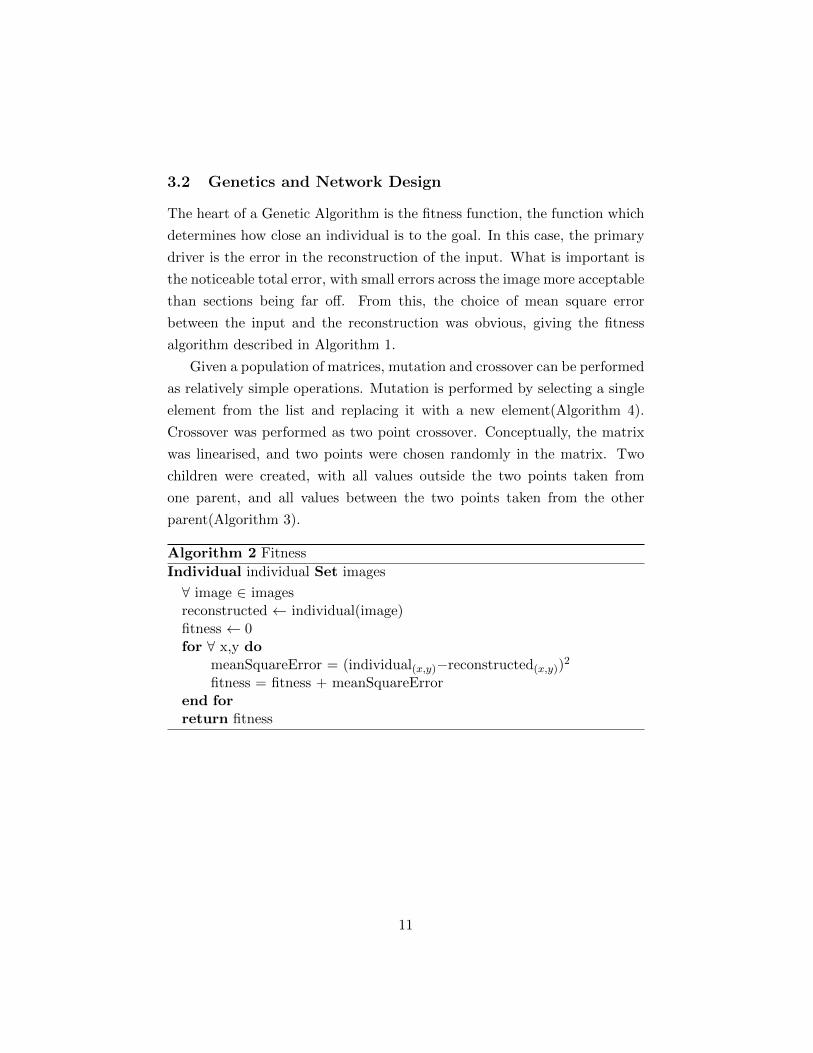
3.2 Genetics and Network Design

The heart of a Genetic Algorithm is the fitness function, the function which

determines how close an individual is to the goal. In this case, the primary

driver is the error in the reconstruction of the input. What is important is

the noticeable total error, with small errors across the image more acceptable

than sections being far off. From this, the choice of mean square error

between the input and the reconstruction was obvious, giving the fitness

algorithm described in Algorithm 1.

Given a population of matrices, mutation and crossover can be performed

as relatively simple operations. Mutation is performed by selecting a single

element from the list and replacing it with a new element(Algorithm 4).

Crossover was performed as two point crossover. Conceptually, the matrix

was linearised, and two points were chosen randomly in the matrix. Two

children were created, with all values outside the two points taken from

one parent, and all values between the two points taken from the other

parent(Algorithm 3).

Algorithm 2 Fitness

Individual individual Set images

∀ image ∈ imagesreconstructed ← individual(image)fitness ← 0for ∀ x,y do

meanSquareError = (individual(x,y)−reconstructed(x,y))2

fitness = fitness + meanSquareErrorend forreturn fitness

11

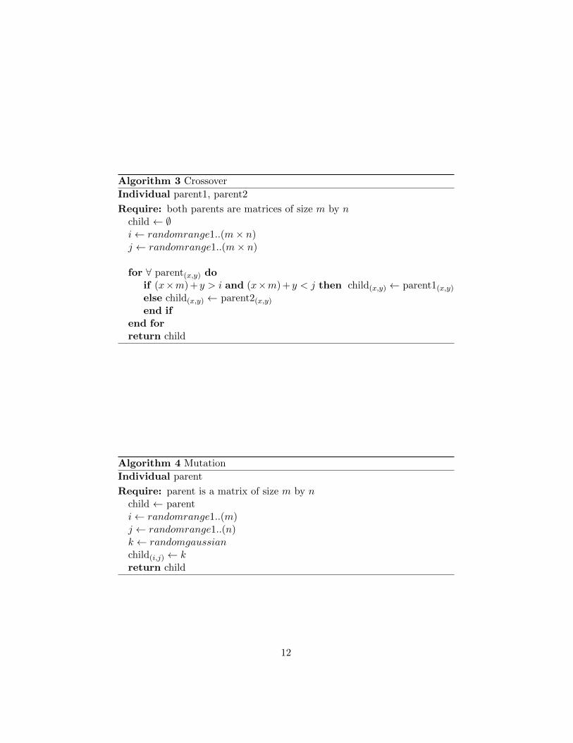
Algorithm 3 Crossover

Individual parent1, parent2

Require: both parents are matrices of size m by nchild ← ∅i← randomrange1..(m× n)j ← randomrange1..(m× n)

for ∀ parent(x,y) doif (x×m) + y > i and (x×m) + y < j then child(x,y) ← parent1(x,y)else child(x,y) ← parent2(x,y)end if

end forreturn child

Algorithm 4 Mutation

Individual parent

Require: parent is a matrix of size m by nchild ← parenti← randomrange1..(m)j ← randomrange1..(n)k ← randomgaussianchild(i,j) ← kreturn child

12

3.3 Sparse Network Design

Once testing had begun, a pattern in the successful children emerged. Most

of the values in the matrices were very close to zero. This becomes apparent

looking at the degenerate case where the difference in size between the input

and the output matrix is 0. The optimal matrix in this case is the identity

matrix, which contains only one non-zero entry per row.

Using this assumption, the genetic sequence of an individual can be

reworked. Instead of generating and keeping an entire matrix, a list of non-

zero elements can be kept and computed. This saves both space, in reducing

the amount of data needed to store the matrix, and the time complexity of

computing the matrix multiplication.

In the new model, each non-zero element is a gene. Instead of a fixed

size genotype, a variable sized genotype, made up of the non-zero elements

in the matrix, is used. Each gene contains a row and column index as to

where it would be in the matrix, and a magnitude. The initial population

is composed of individuals with one randomly chosen gene. Crossover can

increase the length of the genotype, while mutation does not change the

genotype length. A penalty has to be added to the fitness to discourage

trivial additions to the genotype. This penalty must remain relatively small

to not discourage creation of more correct networks, but large enough to

remove extraneous elements. The updated fitness calculation can be seen in

Algorithm 5.

Though this makes computation faster, it complicates mutation and

crossover. The first important change is in the varying of the size of the

matrices. Adding a new element during mutation would be a relatively

large change, changing both the number of non-zero elements and adding a

new element chosen at random. Because of this, altering the size of the gene

list falls to the crossover operator. Meanwhile the mutation operator needs

to mutate more intelligently.

Mutation using the sparse network is a two step process. The child is

created first by removing a gene from the parent, and then adding a new

gene, with randomly chosen position and magnitude, to the child. This can

13

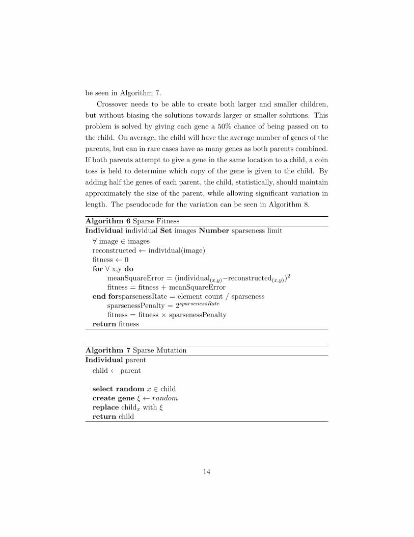
be seen in Algorithm 7.

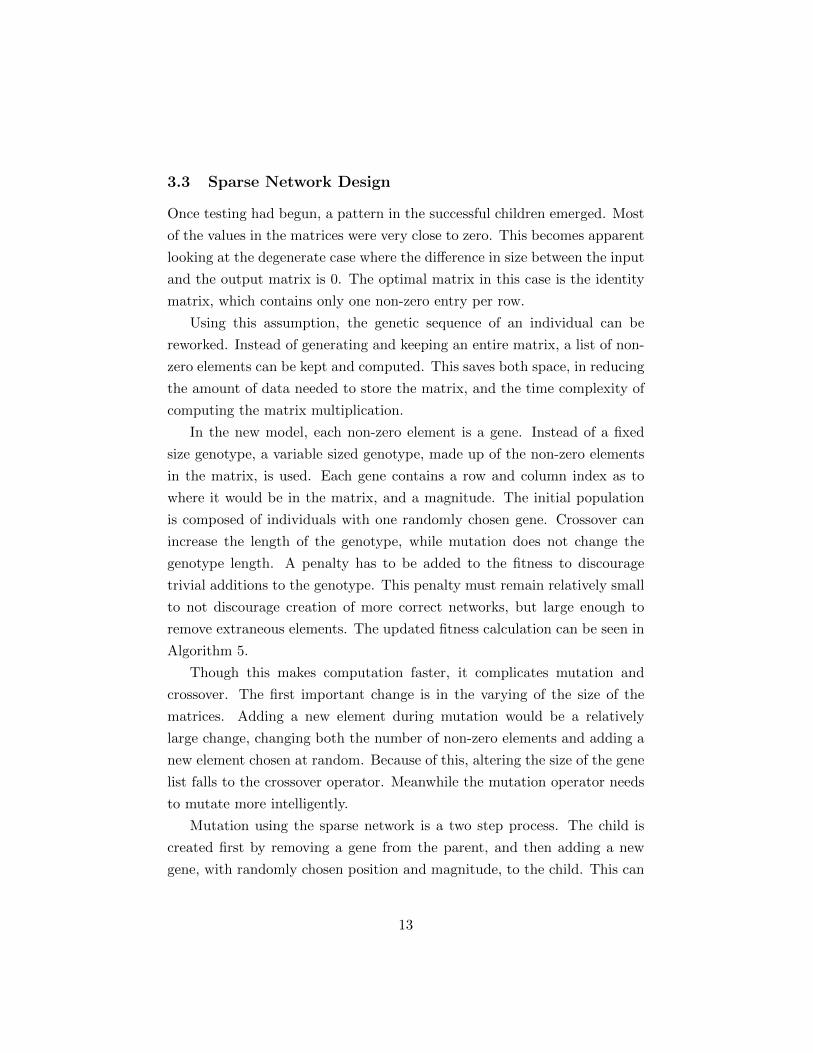
Crossover needs to be able to create both larger and smaller children,

but without biasing the solutions towards larger or smaller solutions. This

problem is solved by giving each gene a 50% chance of being passed on to

the child. On average, the child will have the average number of genes of the

parents, but can in rare cases have as many genes as both parents combined.

If both parents attempt to give a gene in the same location to a child, a coin

toss is held to determine which copy of the gene is given to the child. By

adding half the genes of each parent, the child, statistically, should maintain

approximately the size of the parent, while allowing significant variation in

length. The pseudocode for the variation can be seen in Algorithm 8.

Algorithm 6 Sparse Fitness

Individual individual Set images Number sparseness limit

∀ image ∈ imagesreconstructed ← individual(image)fitness ← 0for ∀ x,y do

meanSquareError = (individual(x,y)−reconstructed(x,y))2

fitness = fitness + meanSquareErrorend forsparsenessRate = element count / sparseness

sparsenessPenalty = 2sparsenessRate

fitness = fitness × sparsenessPenaltyreturn fitness

Algorithm 7 Sparse Mutation

Individual parent

child ← parent

select random x ∈ childcreate gene ξ ← randomreplace childx with ξreturn child

14

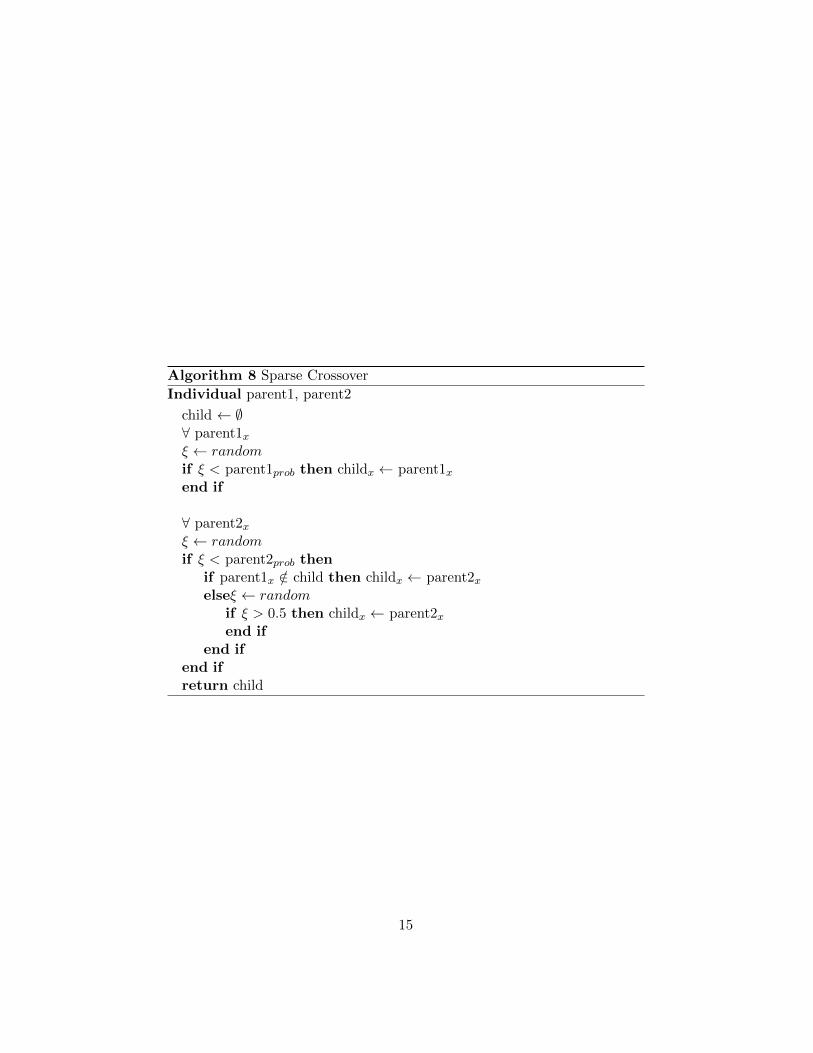
Algorithm 8 Sparse Crossover

Individual parent1, parent2

child ← ∅∀ parent1xξ ← randomif ξ < parent1prob then childx ← parent1xend if

∀ parent2xξ ← randomif ξ < parent2prob then

if parent1x /∈ child then childx ← parent2xelseξ ← random

if ξ > 0.5 then childx ← parent2xend if

end ifend ifreturn child

15

4 Results

The algorithm was trained and tested on greyscale image data, with each

value being normalized in the floating point range 0.0 to 1.0. This data, as

a set of vectors, was used as the input to the algorithm. The reconstruction

of the algorithm was used to determine the fitness of the individuals. See

Section 3.2 and Algorithm 1 for a discussion of the use and calculation of

fitness.

4.1 Parameters

During testing of the data, many ideas were used to attempt to minimise

the time used by the algorithm.

4.1.1 Mutation

An early attempt to increase the convergence rate of the algorithm was

to increase the number of genes mutated with each mutation. This was

successful in the short term, giving faster reduction in the first few moments.

However, these gains were not sustainable, and the algorithm quickly slowed,

ending with a significantly worse reproduction of the image in any non-trivial

test. The early gains suggest that a heuristic approach, e.g. Simulated

Annealing, to varying mutation rates may increase performance.

4.1.2 Elitism

When using a Genetic Algorithm, ensuring high fitness values among the

population is important. However, if a large group of individuals become

very similar. As these similar individuals replace members of the population,

the diversity of the population decreases. This can be mitigated by removing

old members of the population. Removing elitism, the ability of very old

individuals to compete with a new generation, can work to reduce the delay

of local minima, however testing in this problem space did not show any

improvement.

16

4.1.3 Enforced Sparseness

As this algorithm has a variable length genetic code, and the length of a

member of the population changes the computational complexity of the fit-

ness calculation, it is reasonable to conclude that a barrier on the complexity

of the length of the genotype would increase the accuracy of the solution,

to a point. However, simply adding a maximum percentage non-sparseness

limits solutions which may be better using more than the maximum number

of non-zero elements.

A compromise, where the individual was penalized for using non-zero

elements was tested, where each gene gave an ever increasing penalty to

the fitness of the solution. This penalty was multiplied by the error in

the solution, thus making even small improvements capable of reducing the

overall fitness value, even in individuals with large numbers of genes.

When the penalty value was scaled well, this resulted in solutions which

converged in approximately the same number of generations, but signifi-

cantly faster in total computation time.

Results dropped off somewhat when the penalty was very small, but kept

a noticeable improvement in the overall computation speed. However, if the

penalty was large, the computation would fail to find a good solution.

4.1.4 Multithreading

The bulk of the application’s running time was spent in the generation of

fitness values. Placing each fitness calculation into a thread, and calculating

the values simultaneously, resulted in a significant increase in the speed of

calculations on multi-threaded systems, with only a minor change to the

underlying code. On smaller examples, this speed-up was nearly linear, but

as the size of the inputs and resulting matrices increased, the bottleneck

moved to memory on the test machines.

4.1.5 Selection Method

The selection of individuals to keep and to remove from a population is an

important factor to the design of a genetic algorithm. The simplest choice,

17

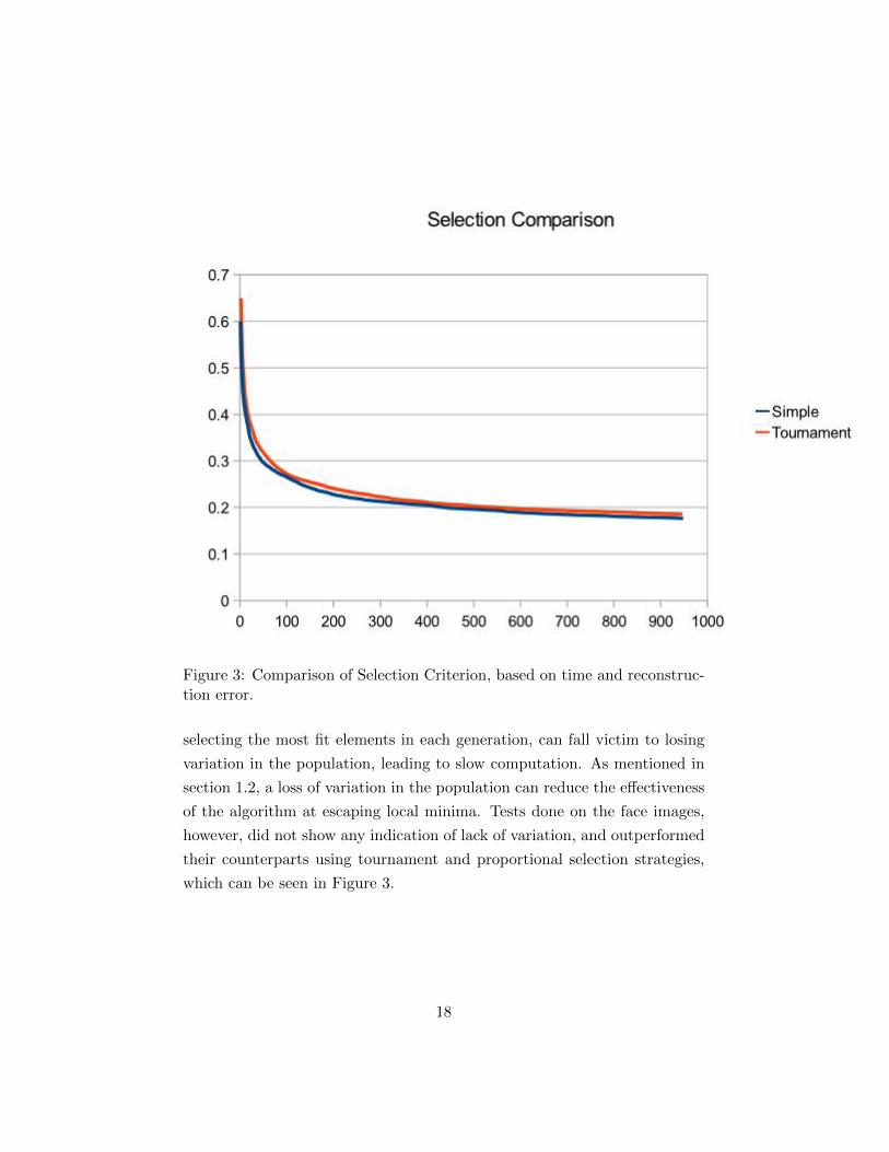
Figure 3: Comparison of Selection Criterion, based on time and reconstruc-tion error.

selecting the most fit elements in each generation, can fall victim to losing

variation in the population, leading to slow computation. As mentioned in

section 1.2, a loss of variation in the population can reduce the effectiveness

of the algorithm at escaping local minima. Tests done on the face images,

however, did not show any indication of lack of variation, and outperformed

their counterparts using tournament and proportional selection strategies,

which can be seen in Figure 3.

18

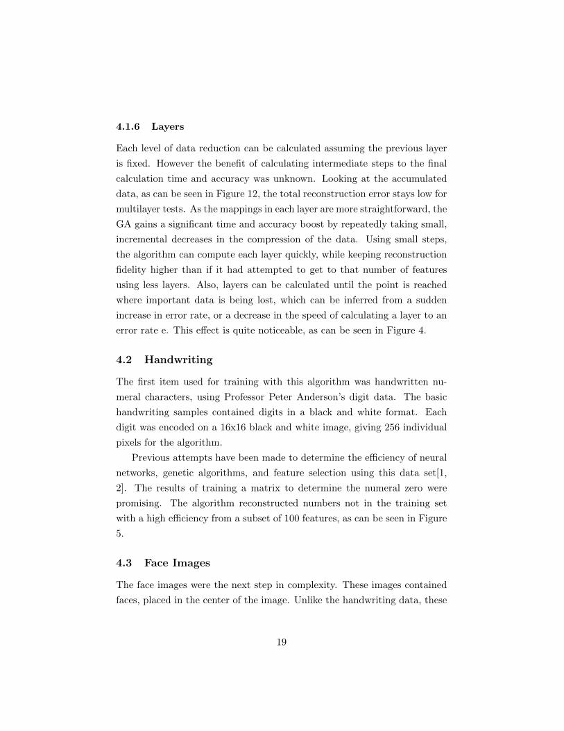
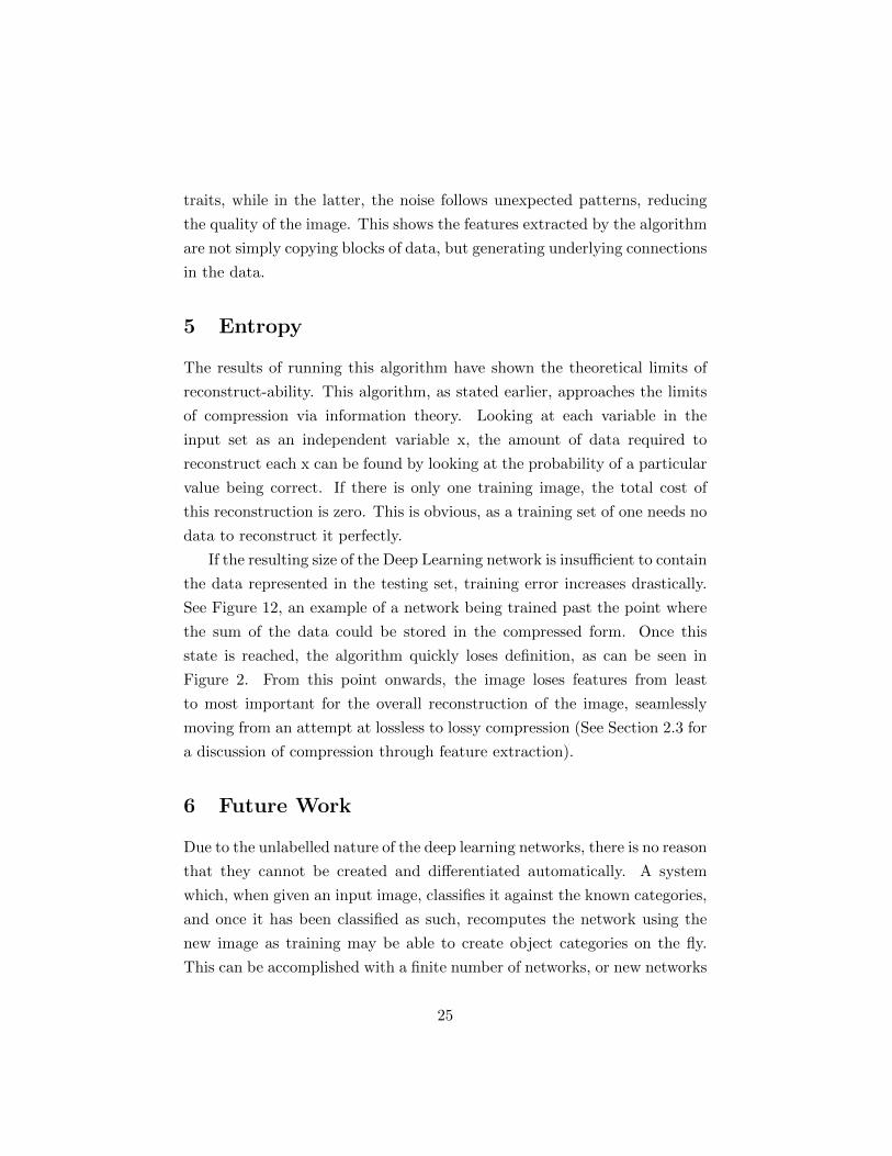
4.1.6 Layers

Each level of data reduction can be calculated assuming the previous layer

is fixed. However the benefit of calculating intermediate steps to the final

calculation time and accuracy was unknown. Looking at the accumulated

data, as can be seen in Figure 12, the total reconstruction error stays low for

multilayer tests. As the mappings in each layer are more straightforward, the

GA gains a significant time and accuracy boost by repeatedly taking small,

incremental decreases in the compression of the data. Using small steps,

the algorithm can compute each layer quickly, while keeping reconstruction

fidelity higher than if it had attempted to get to that number of features

using less layers. Also, layers can be calculated until the point is reached

where important data is being lost, which can be inferred from a sudden

increase in error rate, or a decrease in the speed of calculating a layer to an

error rate e. This effect is quite noticeable, as can be seen in Figure 4.

4.2 Handwriting

The first item used for training with this algorithm was handwritten nu-

meral characters, using Professor Peter Anderson’s digit data. The basic

handwriting samples contained digits in a black and white format. Each

digit was encoded on a 16x16 black and white image, giving 256 individual

pixels for the algorithm.

Previous attempts have been made to determine the efficiency of neural

networks, genetic algorithms, and feature selection using this data set[1,

2]. The results of training a matrix to determine the numeral zero were

promising. The algorithm reconstructed numbers not in the training set

with a high efficiency from a subset of 100 features, as can be seen in Figure

5.

4.3 Face Images

The face images were the next step in complexity. These images contained

faces, placed in the center of the image. Unlike the handwriting data, these

19

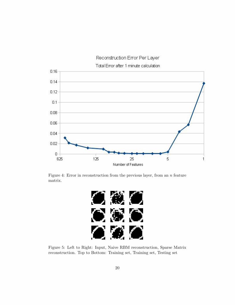
Figure 4: Error in reconstruction from the previous layer, from an n featurematrix.

Figure 5: Left to Right: Input, Naive RBM reconstruction, Sparse Matrixreconstruction. Top to Bottom: Training set, Training set, Testing set

20

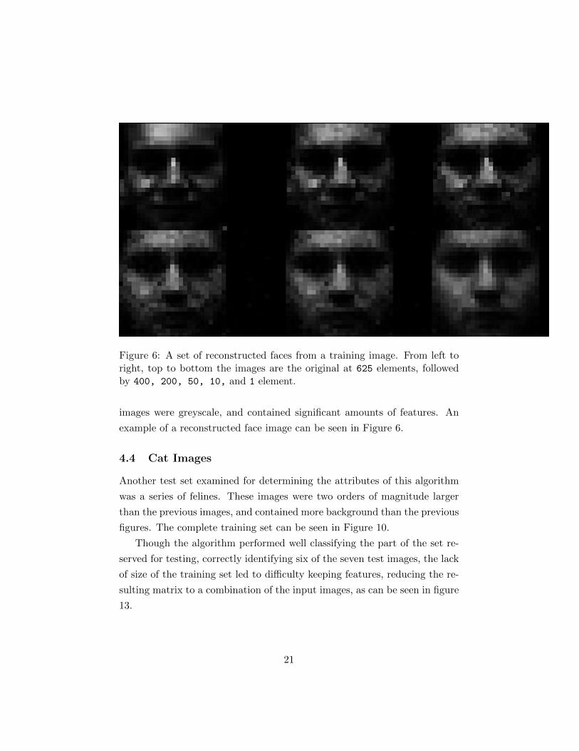
Figure 6: A set of reconstructed faces from a training image. From left toright, top to bottom the images are the original at 625 elements, followedby 400, 200, 50, 10, and 1 element.

images were greyscale, and contained significant amounts of features. An

example of a reconstructed face image can be seen in Figure 6.

4.4 Cat Images

Another test set examined for determining the attributes of this algorithm

was a series of felines. These images were two orders of magnitude larger

than the previous images, and contained more background than the previous

figures. The complete training set can be seen in Figure 10.

Though the algorithm performed well classifying the part of the set re-

served for testing, correctly identifying six of the seven test images, the lack

of size of the training set led to difficulty keeping features, reducing the re-

sulting matrix to a combination of the input images, as can be seen in figure

13.

21

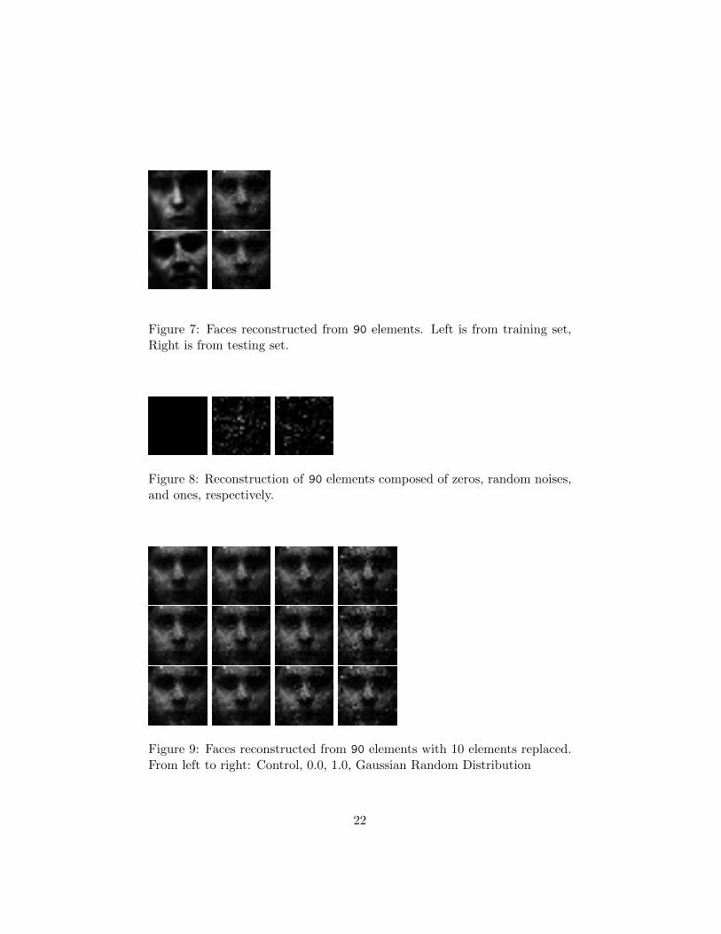
Figure 7: Faces reconstructed from 90 elements. Left is from training set,Right is from testing set.

Figure 8: Reconstruction of 90 elements composed of zeros, random noises,and ones, respectively.

Figure 9: Faces reconstructed from 90 elements with 10 elements replaced.From left to right: Control, 0.0, 1.0, Gaussian Random Distribution

22

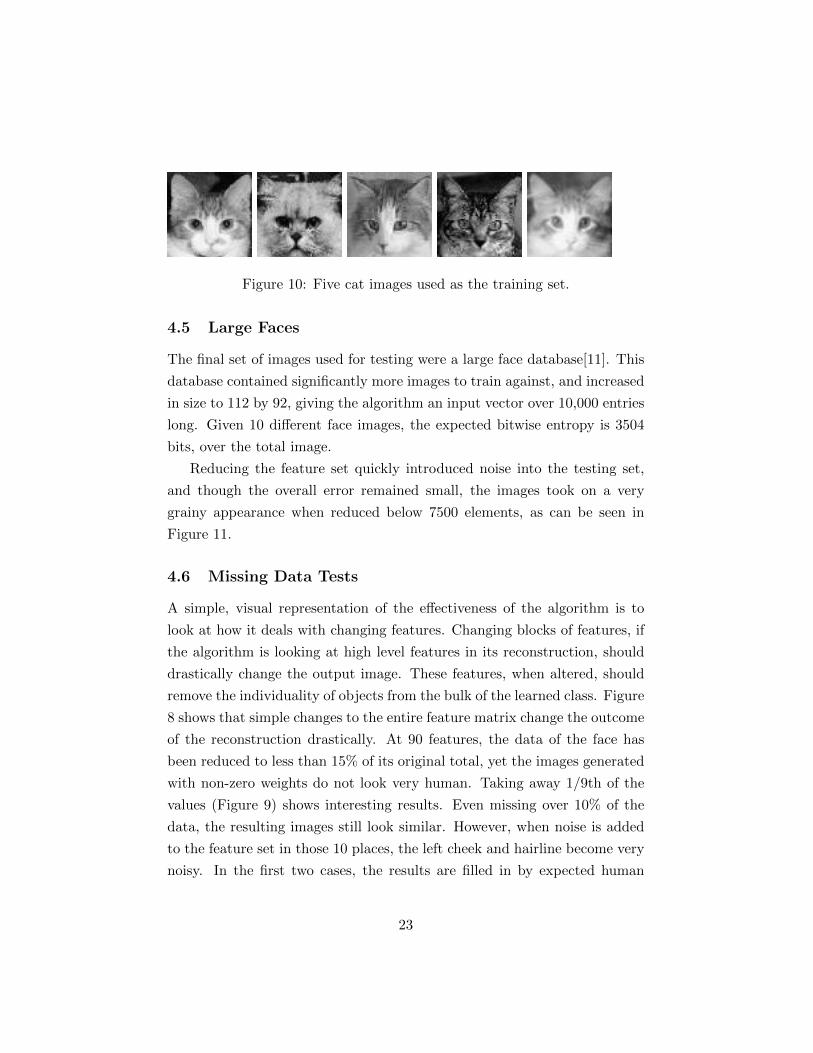
Figure 10: Five cat images used as the training set.

4.5 Large Faces

The final set of images used for testing were a large face database[11]. This

database contained significantly more images to train against, and increased

in size to 112 by 92, giving the algorithm an input vector over 10,000 entries

long. Given 10 different face images, the expected bitwise entropy is 3504

bits, over the total image.

Reducing the feature set quickly introduced noise into the testing set,

and though the overall error remained small, the images took on a very

grainy appearance when reduced below 7500 elements, as can be seen in

Figure 11.

4.6 Missing Data Tests

A simple, visual representation of the effectiveness of the algorithm is to

look at how it deals with changing features. Changing blocks of features, if

the algorithm is looking at high level features in its reconstruction, should

drastically change the output image. These features, when altered, should

remove the individuality of objects from the bulk of the learned class. Figure

8 shows that simple changes to the entire feature matrix change the outcome

of the reconstruction drastically. At 90 features, the data of the face has

been reduced to less than 15% of its original total, yet the images generated

with non-zero weights do not look very human. Taking away 1/9th of the

values (Figure 9) shows interesting results. Even missing over 10% of the

data, the resulting images still look similar. However, when noise is added

to the feature set in those 10 places, the left cheek and hairline become very

noisy. In the first two cases, the results are filled in by expected human

23

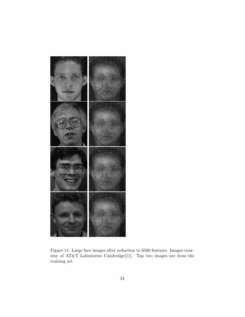
Figure 11: Large face images after reduction to 6500 features. Images cour-tesy of AT&T Labratories Cambridge[11]. Top two images are from thetraining set.

24

traits, while in the latter, the noise follows unexpected patterns, reducing

the quality of the image. This shows the features extracted by the algorithm

are not simply copying blocks of data, but generating underlying connections

in the data.

5 Entropy

The results of running this algorithm have shown the theoretical limits of

reconstruct-ability. This algorithm, as stated earlier, approaches the limits

of compression via information theory. Looking at each variable in the

input set as an independent variable x, the amount of data required to

reconstruct each x can be found by looking at the probability of a particular

value being correct. If there is only one training image, the total cost of

this reconstruction is zero. This is obvious, as a training set of one needs no

data to reconstruct it perfectly.

If the resulting size of the Deep Learning network is insufficient to contain

the data represented in the testing set, training error increases drastically.

See Figure 12, an example of a network being trained past the point where

the sum of the data could be stored in the compressed form. Once this

state is reached, the algorithm quickly loses definition, as can be seen in

Figure 2. From this point onwards, the image loses features from least

to most important for the overall reconstruction of the image, seamlessly

moving from an attempt at lossless to lossy compression (See Section 2.3 for

a discussion of compression through feature extraction).

6 Future Work

Due to the unlabelled nature of the deep learning networks, there is no reason

that they cannot be created and differentiated automatically. A system

which, when given an input image, classifies it against the known categories,

and once it has been classified as such, recomputes the network using the

new image as training may be able to create object categories on the fly.

This can be accomplished with a finite number of networks, or new networks

25

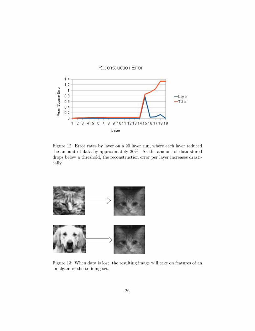
Figure 12: Error rates by layer on a 20 layer run, where each layer reducedthe amount of data by approximately 20%. As the amount of data storeddrops below a threshold, the reconstruction error per layer increases drasti-cally.

Figure 13: When data is lost, the resulting image will take on features of anamalgam of the training set.

26

can be created when the classification falls above a certain threshold, thus

creating an adaptive network of object classifications, independent of user

input. This can allow an algorithm to create and classify new object types

on the fly, with the fluidity of more robust data mining applications, while

maintaining the speed and flexibility of computation of the deep learning

network.

As stated earlier, this algorithm does not take any specific optimizations

for the domain of imaging, and can work without change with any domain

based on fixed length sets of floating point data. With domain specific

optimizations, it may perform significantly better within its domain.

References

[1] Anderson, P., Gaborski, R., Tilley, D., & Asbury, C.(1993). ”GeneticAlgorithm Selection of Features for Handwritten Character Identifica-tion.” Artificial Neural Nets and Genetic Algorithms. Proceedings ofthe International Conference.

[2] Anderson, P. , & Gaborski, R. (1993). The polynomial method aug-mented by supervised training for hand-printed character recognition.Artificial Neural Nets and Genetic Algorithms. Proceedings of the In-ternational Conference, 101-106.

[3] Arel, I. , Rose, D. , & Karnowski, T. (2010). Deep machine learning-a new frontier in artificial intelligence research. Ieee ComputationalIntelligence Magazine, 5(4), 13-18.

[4] Baeck, T. , Hammel, U. , & Schwefel, H. (1997). Evolutionary compu-tation: Comments on the history and current state. IEEE Transactionson Evolutionary Computation, 1(1), 3-17.

[5] Bengio, Y. (2009). Learning Deep Architectures for AI (Vol. 2, pp. 127).Foundations and Trends in Machine Learning.

[6] Deep Learning. (2006). Retrieved April 15th, 2012, fromhttp://deeplearning.net/

[7] De Jong, K. A. (2006). Evolutionary computation : a unified approach.Cambridge, Mass.: MIT Press.

27

[8] Hinton, G. (2010). A Practical Guide to Training Restricted BoltzmannMachines (Version 1 ed.). University of Toronto: Department of Com-puter Science.

[9] Hinton, G. , Osindero, S. , & Teh, Y. (2006). A fast learning algorithmfor deep belief nets. Neural Computation, 18(7), 1527-1554

[10] Srinivas, M. , & Patnaik, L. (1994). Genetic algorithms: A survey.Computer, 27(6), 17-26.

[11] The Database of Faces. AT&T LaboratoriesCambridge. Retrieved 4/20/2012, 2012, fromhttp://www.cl.cam.ac.uk/research/dtg/attarchive/facedatabase.html

28