Embed Size (px)
Citation preview

Deep Learning
G6032, G6061, 934G5, 807G5, G5015
Dr. Viktoriia Sharmanska

Content: today
! Deep architectures: short intro
! Deep Convolutional Neural Networks ! Convolutional layer ! Max pooling layer ! Fully connected layer ! Non-linear activation function ReLU
! Case study: AlexNet, winner of ILSVRC’12 ! AlexNet architecture
! Fast-forward to today: Revolution of Depth
2
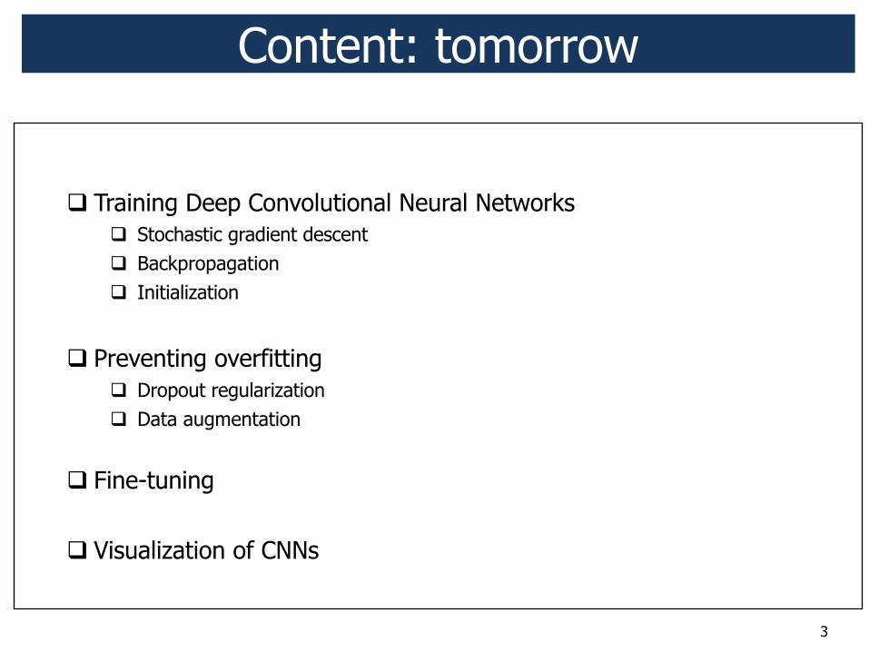
Content: tomorrow
! Training Deep Convolutional Neural Networks
! Stochastic gradient descent ! Backpropagation ! Initialization
! Preventing overfitting
! Dropout regularization ! Data augmentation
! Fine-tuning
! Visualization of CNNs
3
4
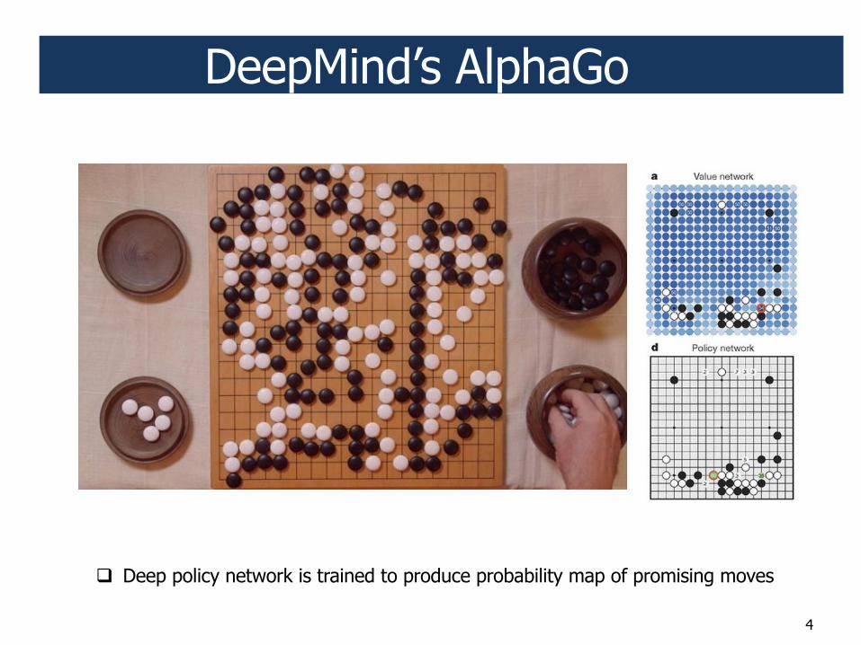
DeepMind’s AlphaGo
! Deep policy network is trained to produce probability map of promising moves
5
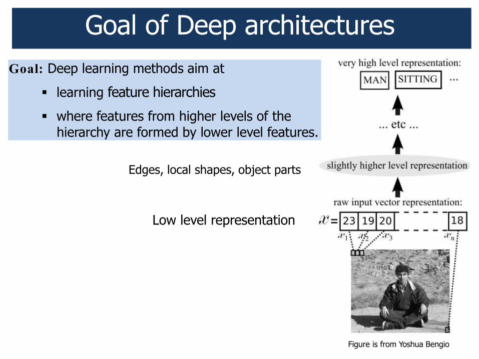
Goal of Deep architectures Goal: Deep learning methods aim at
" learning feature hierarchies
" where features from higher levels of the hierarchy are formed by lower level features.
Figure is from Yoshua Bengio
Low level representation
Edges, local shapes, object parts
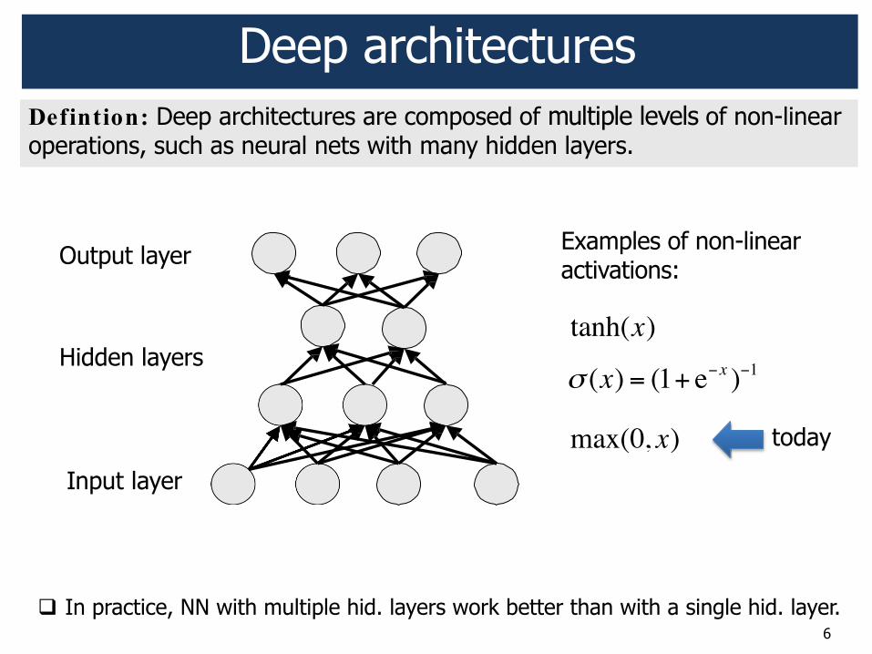
Defintion: Deep architectures are composed of multiple levels of non-linear operations, such as neural nets with many hidden layers.
Deep architectures
Input layer
Output layer
Hidden layers
6
! In practice, NN with multiple hid. layers work better than with a single hid. layer.
Examples of non-linear activations:
max(0, x) today
tanh(x)
! (x) = (1+ e!x )!1
7
Deep Convolutional Networks CNNs
Compared to standard neural networks with similarly-sized layers,
" CNNs have much fewer connections and parameters
" and so they are easier to train
" and typically have more than five layers (a number of layers which makes fully-connected neural networks almost impossible to train properly when initialized randomly)
LeNet, 1998 LeCun Y, Bottou L, Bengio Y, Haffner P: Gradient-Based Learning Applied to Document Recognition, Proceedings of the IEEE
AlexNet, 2012 Krizhevsky A, Sutskever I, Hinton G: ImageNet Classification with Deep Convolutional Neural Networks, NIPS 2012

8
Deep Convolutional Networks
! Convolutional layer ! Non-linear activation function ReLU ! Max pooling layer ! Fully connected layer
9
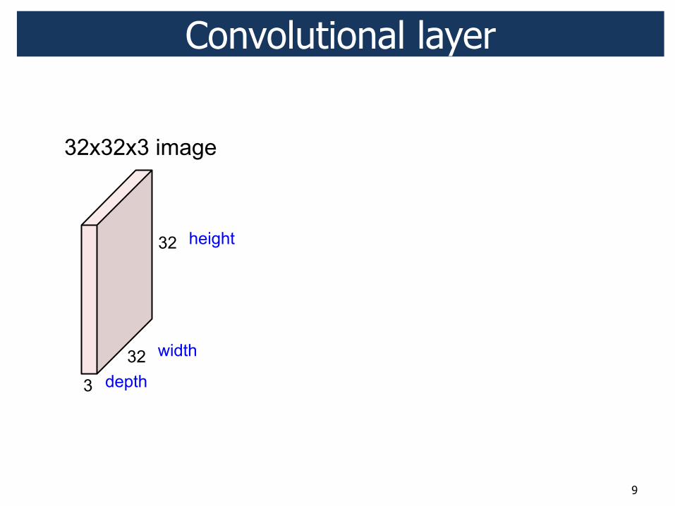
Convolutional layer
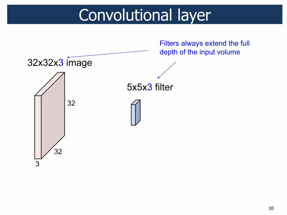
10
Convolutional layer
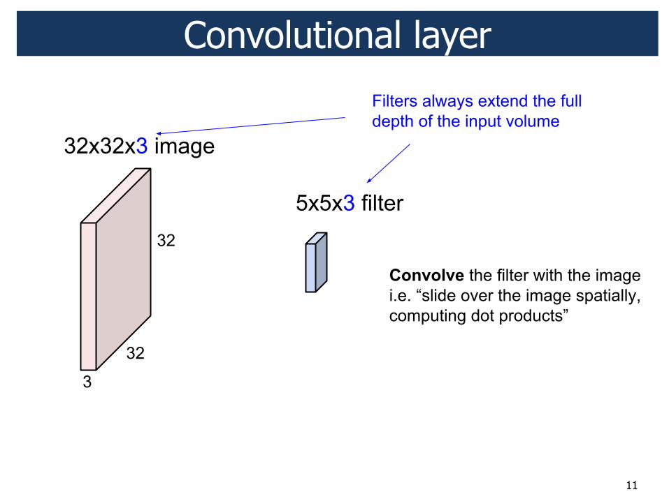
11
Convolutional layer
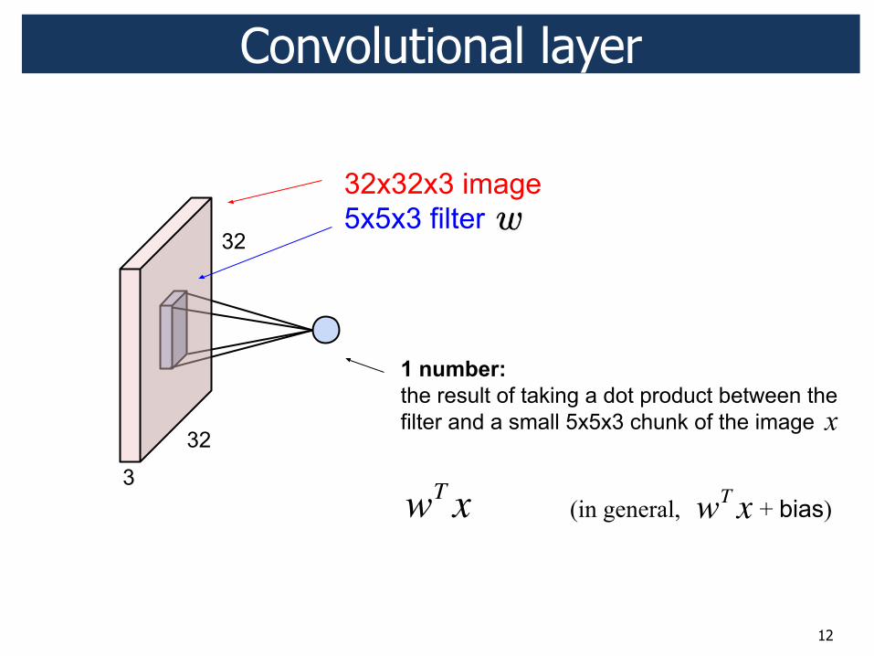
12
Convolutional layer
x
wT x (in general, + bias) wT x
13
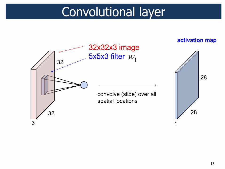
Convolutional layer
w1
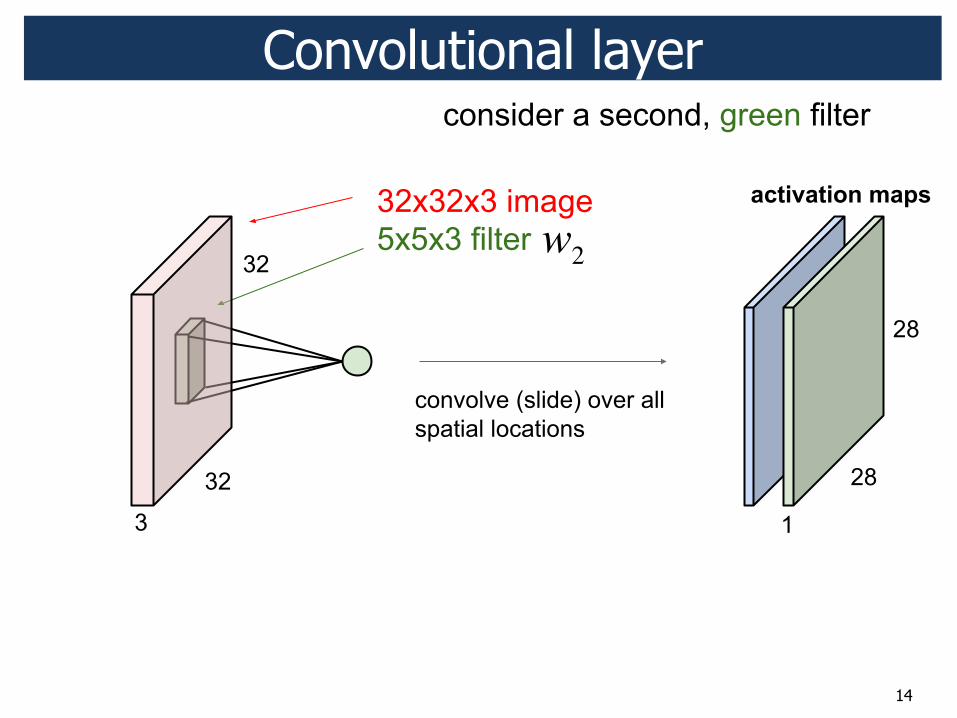
14
Convolutional layer
w2

15
Convolutional layer
x3
16
!"#$%%&'()*+,-./!01,.2%3''4/'%&2+567482%.+749,!/8:;
[Convolution Demo: extra]
17
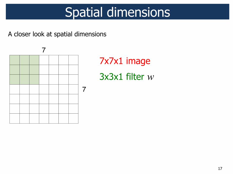
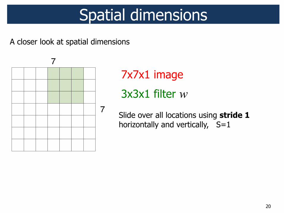
7x7x1 image
3x3x1 filter w
Spatial dimensions
7
7
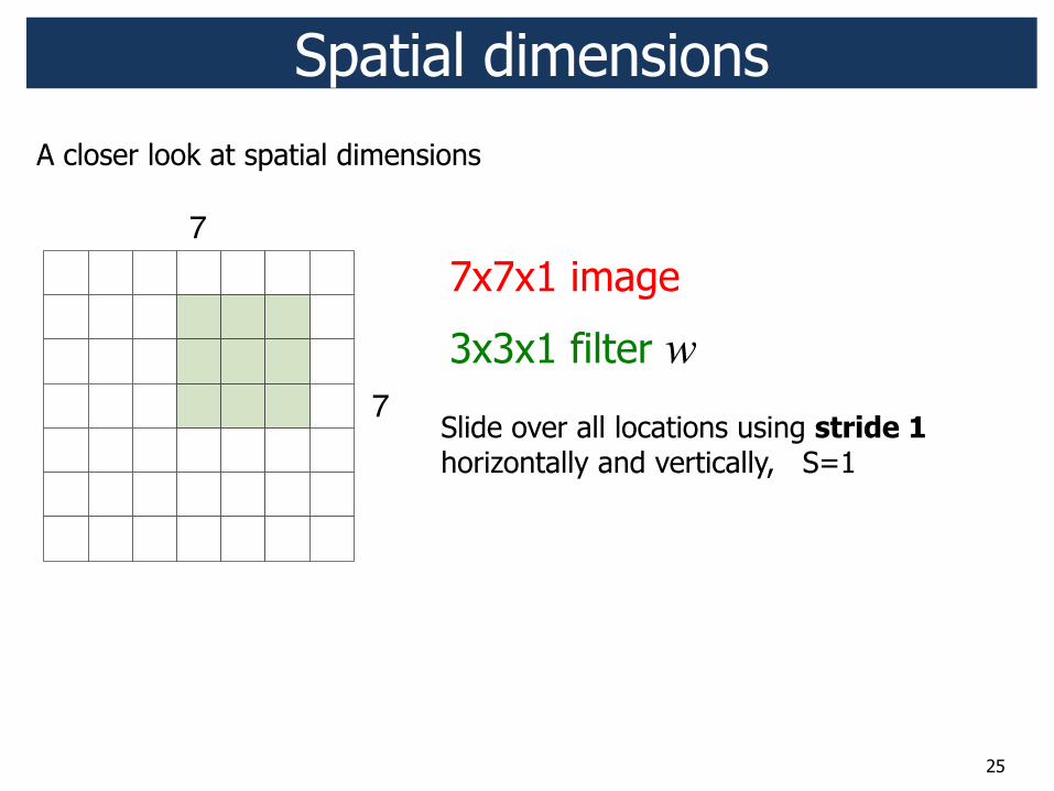
A closer look at spatial dimensions

18
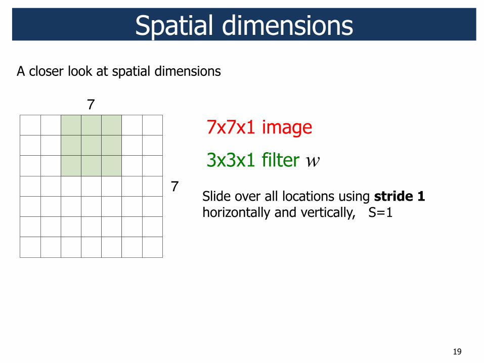
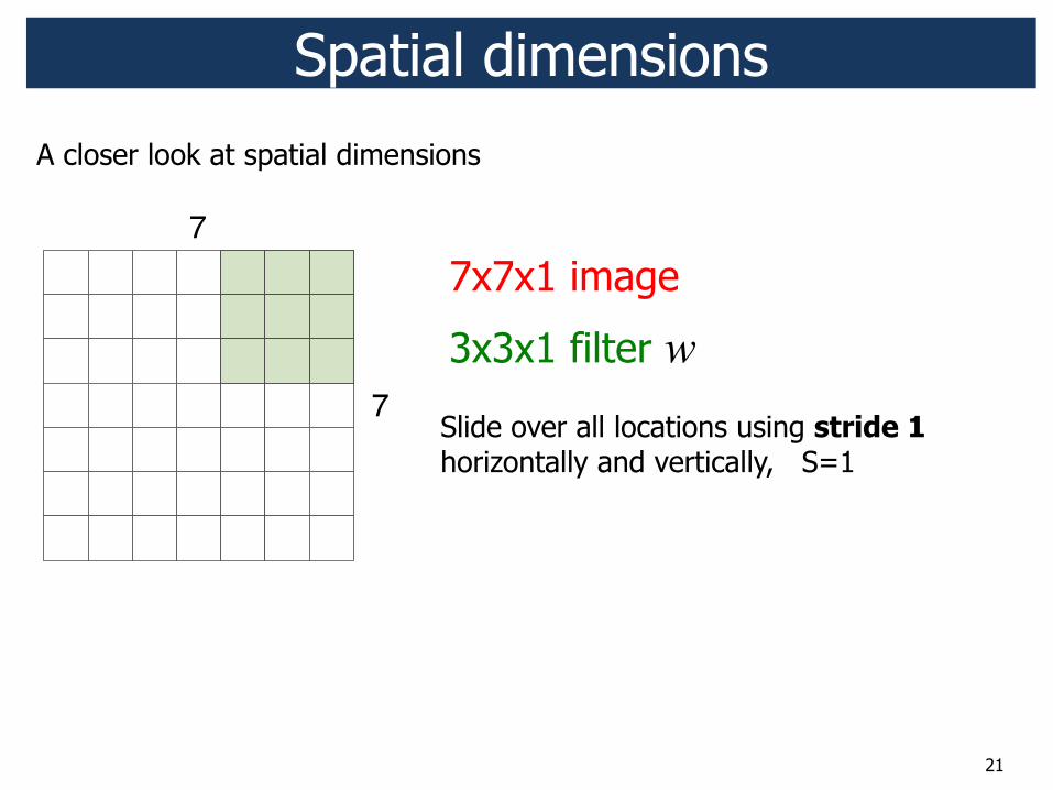
7x7x1 image
3x3x1 filter w
Slide over all locations using stride 1 horizontally and vertically, S=1
Spatial dimensions
7
7
A closer look at spatial dimensions
19
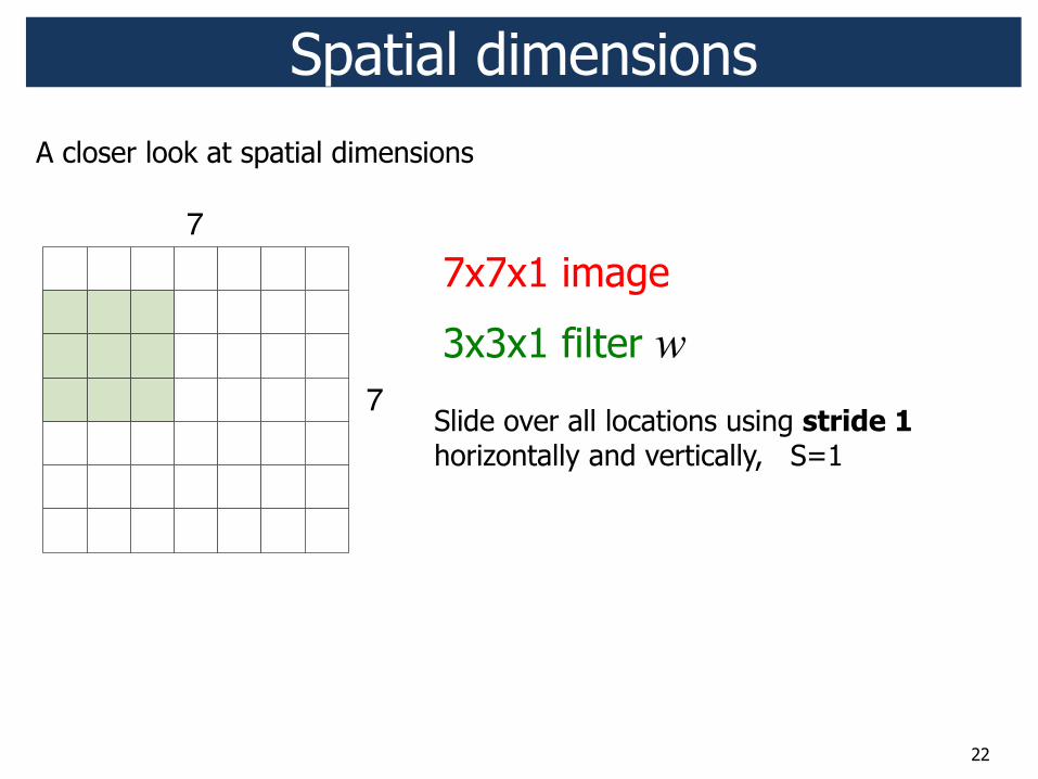
7x7x1 image
3x3x1 filter w
Slide over all locations using stride 1 horizontally and vertically, S=1
Spatial dimensions
7
7
A closer look at spatial dimensions
20
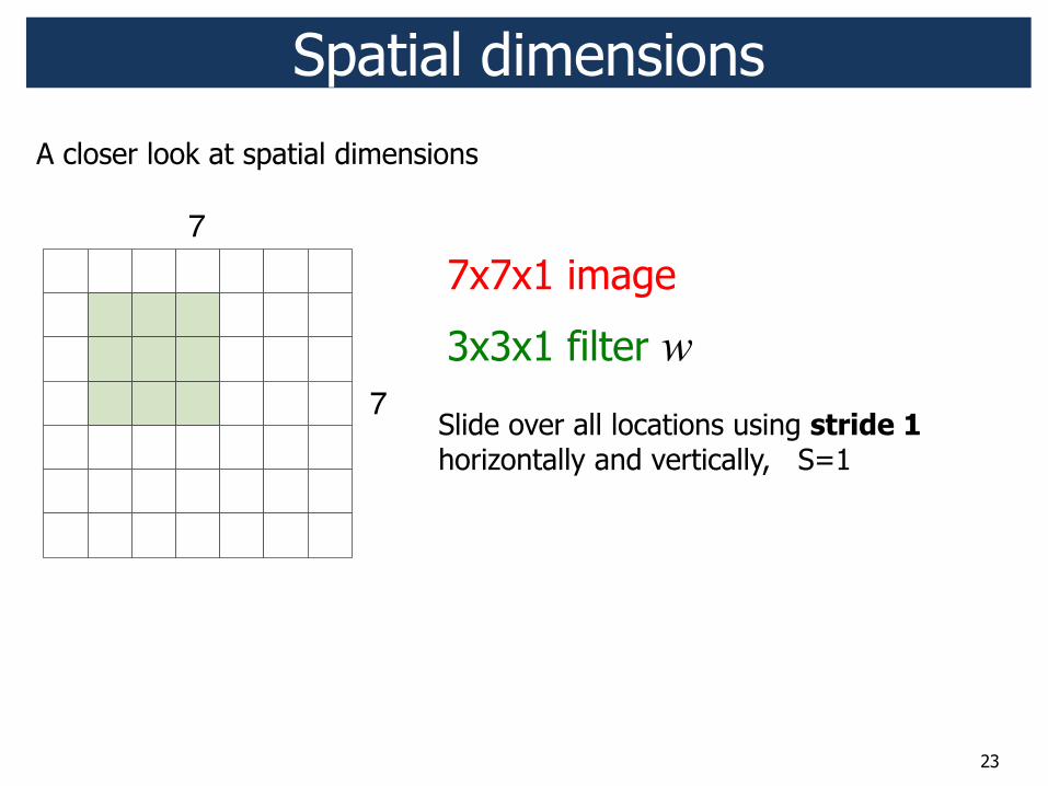
7x7x1 image
3x3x1 filter w
Slide over all locations using stride 1 horizontally and vertically, S=1
Spatial dimensions
7
7
A closer look at spatial dimensions
21
7x7x1 image
3x3x1 filter w
Slide over all locations using stride 1 horizontally and vertically, S=1
Spatial dimensions
7
7
A closer look at spatial dimensions
22
7x7x1 image
3x3x1 filter w
Slide over all locations using stride 1 horizontally and vertically, S=1
Spatial dimensions
7
7
A closer look at spatial dimensions
23
7x7x1 image
3x3x1 filter w
Slide over all locations using stride 1 horizontally and vertically, S=1
Spatial dimensions
7
7
A closer look at spatial dimensions

24
7x7x1 image
3x3x1 filter w
Slide over all locations using stride 1 horizontally and vertically, S=1
Spatial dimensions
7
7
A closer look at spatial dimensions
25
7x7x1 image
3x3x1 filter w
Slide over all locations using stride 1 horizontally and vertically, S=1
Spatial dimensions
7
7
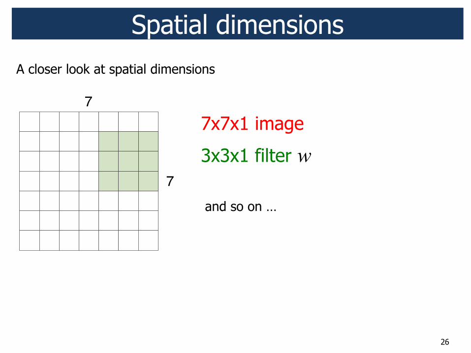
A closer look at spatial dimensions
26
7x7x1 image
3x3x1 filter w
and so on …
Spatial dimensions
7
7
A closer look at spatial dimensions

27
(activation map)
7x7x1 image
3x3x1 filter w stride S=1
! 5x5 output activation map
Spatial dimensions
7
7
A closer look at spatial dimensions
28
7x7x1 image
3x3x1 filter w
Slide over all locations using stride 2 horizontally and vertically, S=2
Spatial dimensions
7
7
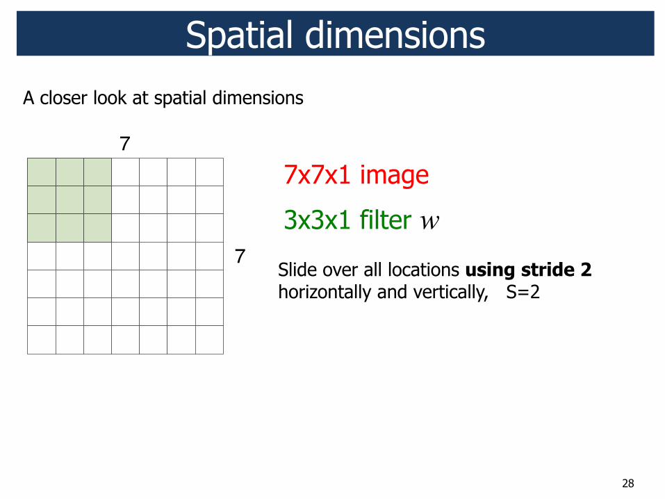
A closer look at spatial dimensions
29
7x7x1 image
3x3x1 filter w
Slide over all locations using stride 2 horizontally and vertically, S=2
Spatial dimensions
7
7
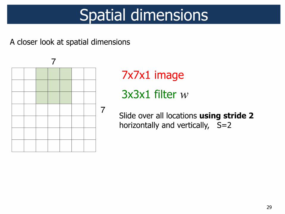
A closer look at spatial dimensions

30
7x7x1 image
3x3x1 filter w
Slide over all locations using stride 2 horizontally and vertically, S=2
Spatial dimensions
7
7
A closer look at spatial dimensions
31
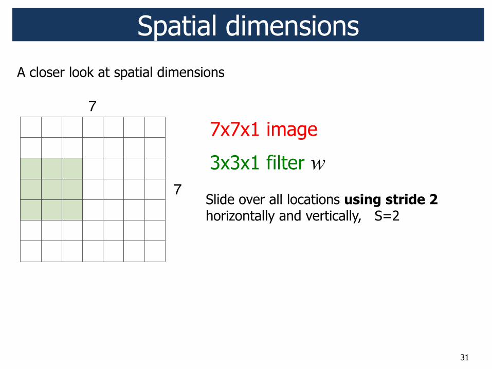
7x7x1 image
3x3x1 filter w
Slide over all locations using stride 2 horizontally and vertically, S=2
Spatial dimensions
7
7
A closer look at spatial dimensions
32
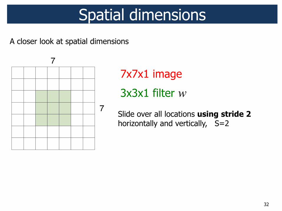
7x7x1 image
3x3x1 filter w
Slide over all locations using stride 2 horizontally and vertically, S=2
Spatial dimensions
7
7
A closer look at spatial dimensions
33
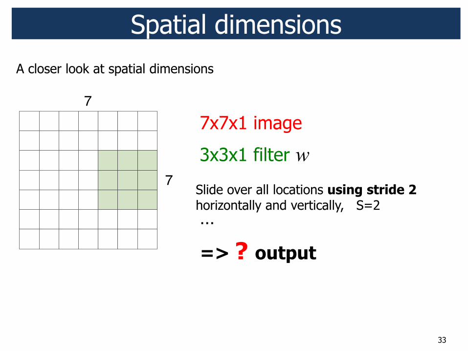
7x7x1 image
3x3x1 filter w
…
=> ? output
Slide over all locations using stride 2 horizontally and vertically, S=2
Spatial dimensions
7
7
A closer look at spatial dimensions
34
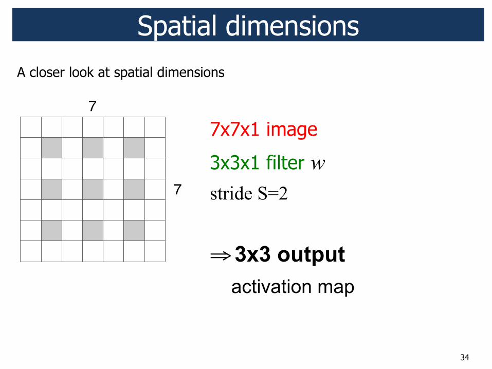
7x7x1 image
3x3x1 filter w stride S=2
! 3x3 output activation map
Spatial dimensions
7
7
A closer look at spatial dimensions
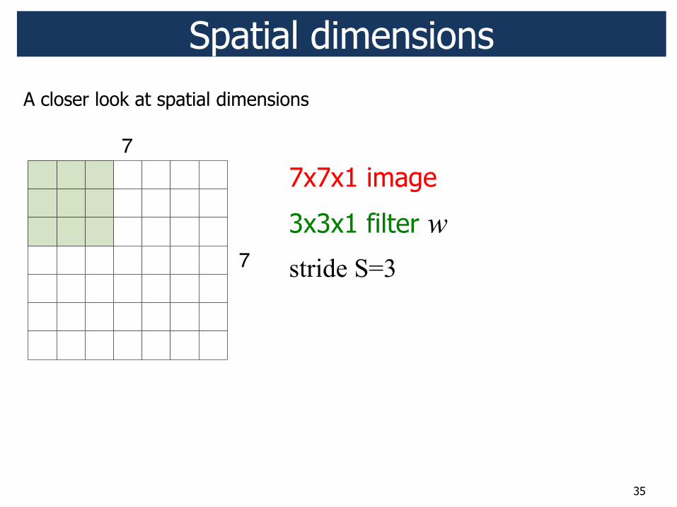
35
7x7x1 image
3x3x1 filter w stride S=3
Spatial dimensions
7
7
A closer look at spatial dimensions
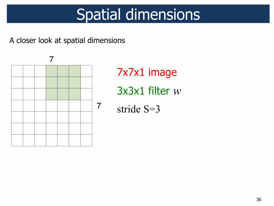
36
7x7x1 image
3x3x1 filter w stride S=3
Spatial dimensions
7
7
A closer look at spatial dimensions
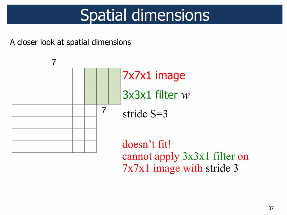
37
7x7x1 image
3x3x1 filter w stride S=3
doesn’t fit! cannot apply 3x3x1 filter on 7x7x1 image with stride 3
Spatial dimensions
7
7
A closer look at spatial dimensions

38
7x7x1 image
3x3x1 filter w stride S=3
?
Spatial dimensions
7
7
A closer look at spatial dimensions
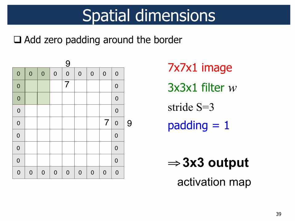
39
7x7x1 image
3x3x1 filter w stride S=3
padding = 1
! 3x3 output activation map
! Add zero padding around the border
Spatial dimensions
9
9
0 0 0 0 0 0 0 0 0
0 0 0 0 0 0 0 0 0
0
0
0
0
0
0
0
0
0
0
0
0
0
0
7
7
7
7
40
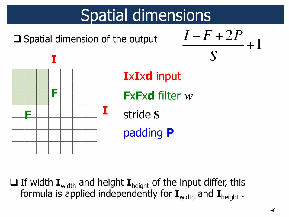
IxIxd input
FxFxd filter w stride S
padding P
Spatial dimensions
F
F
I
I
I !F + 2PS
+1! Spatial dimension of the output
! If width Iwidth and height Iheight of the input differ, this formula is applied independently for Iwidth and Iheight .
41
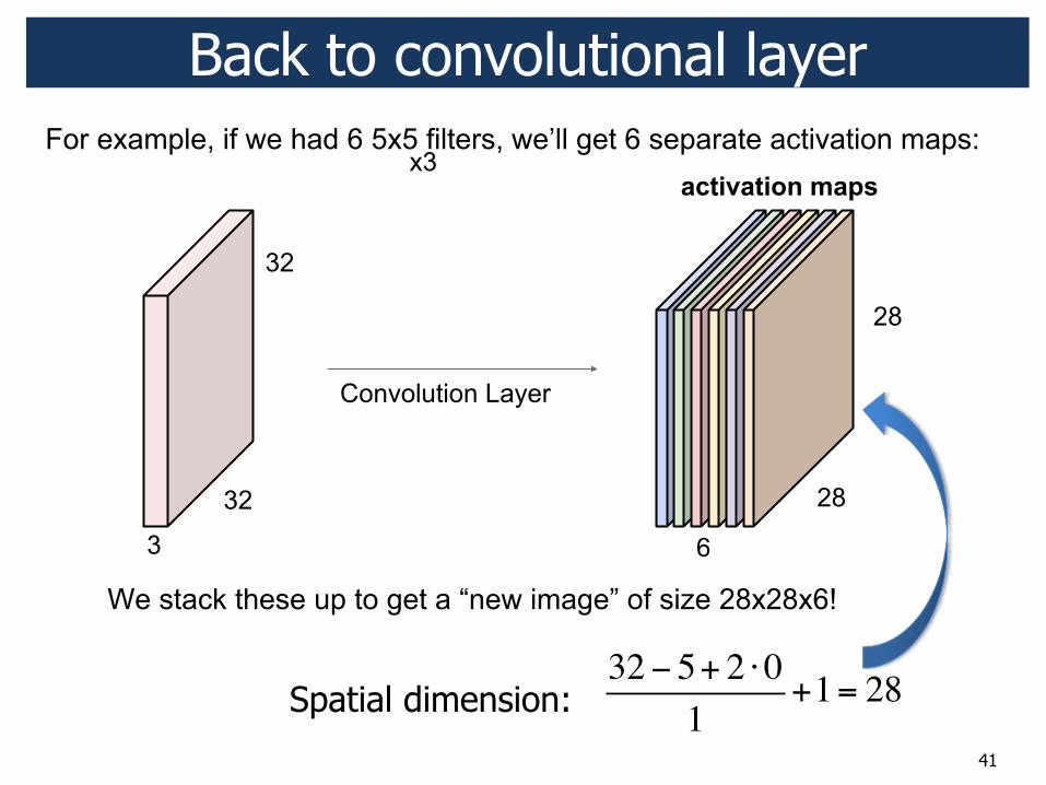
Back to convolutional layer
32! 5+ 2 "01
+1= 28Spatial dimension: ;
x3
42
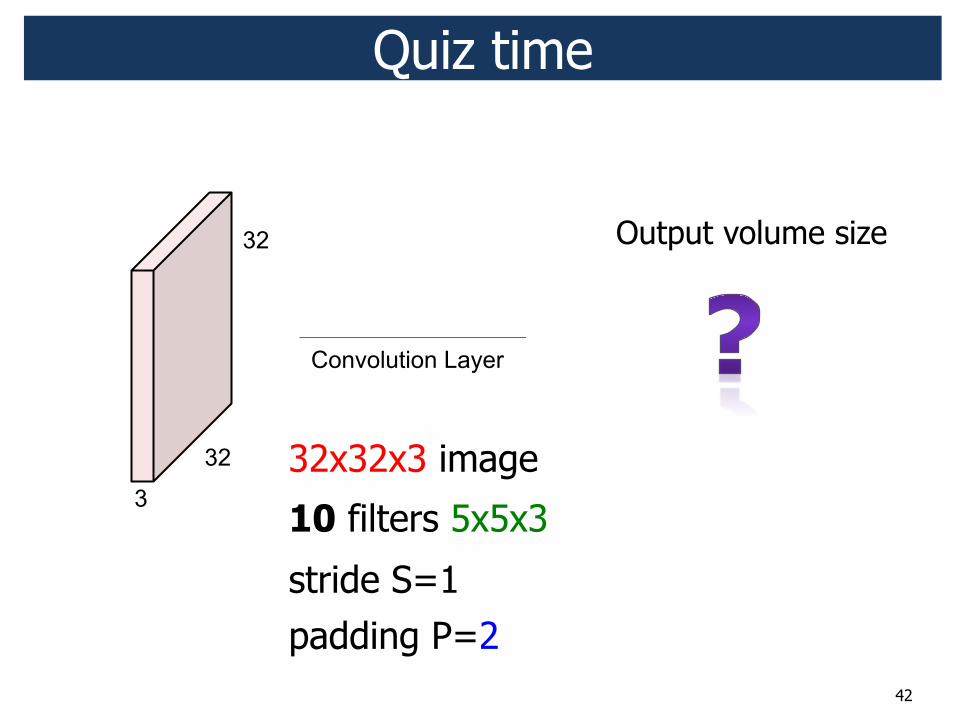
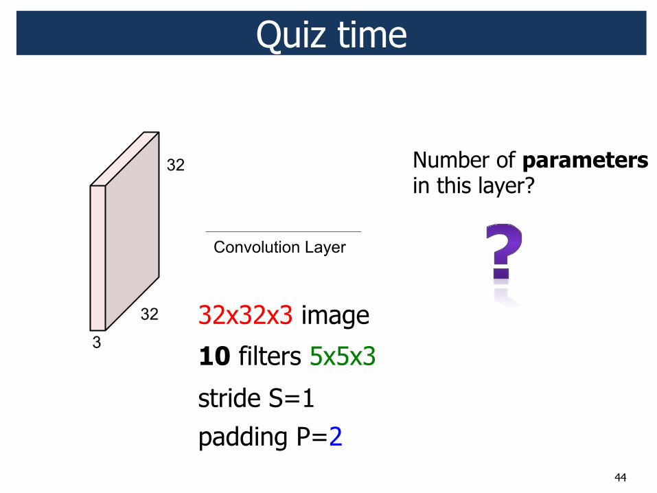
Quiz time
32x32x3 image
10 filters 5x5x3
stride S=1 padding P=2
Output volume size
43
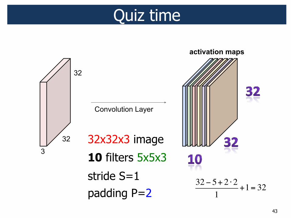
32x32x3 image
10 filters 5x5x3
stride S=1 padding P=2
32! 5+ 2 "21
+1= 32
2 !
2 !!
Quiz time
44
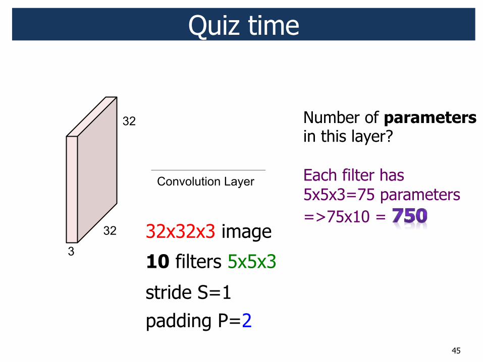
32x32x3 image
10 filters 5x5x3
stride S=1 padding P=2
Number of parameters in this layer?
Quiz time
45
Number of parameters in this layer? Each filter has 5x5x3=75 parameters =>75x10 =
32x32x3 image
10 filters 5x5x3
stride S=1 padding P=2
Quiz time

46
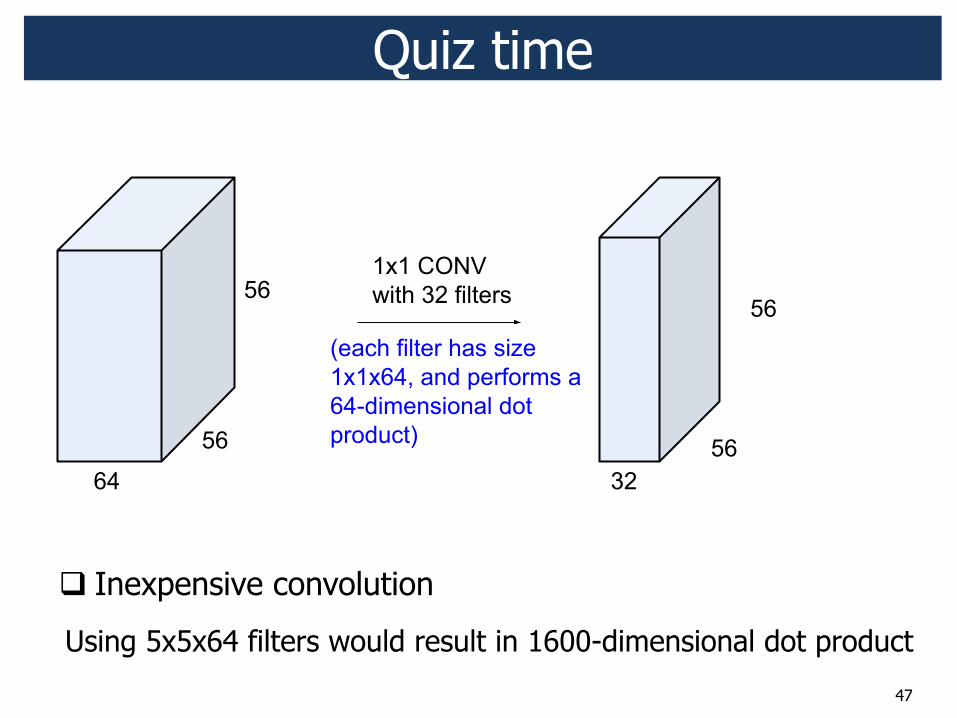
Can we do convolution with 1x1xdepth filter
56x56x64 image
32 filters 1x1x64
S=1, P=0
Quiz time
47
! Inexpensive convolution
Using 5x5x64 filters would result in 1600-dimensional dot product
Quiz time
48
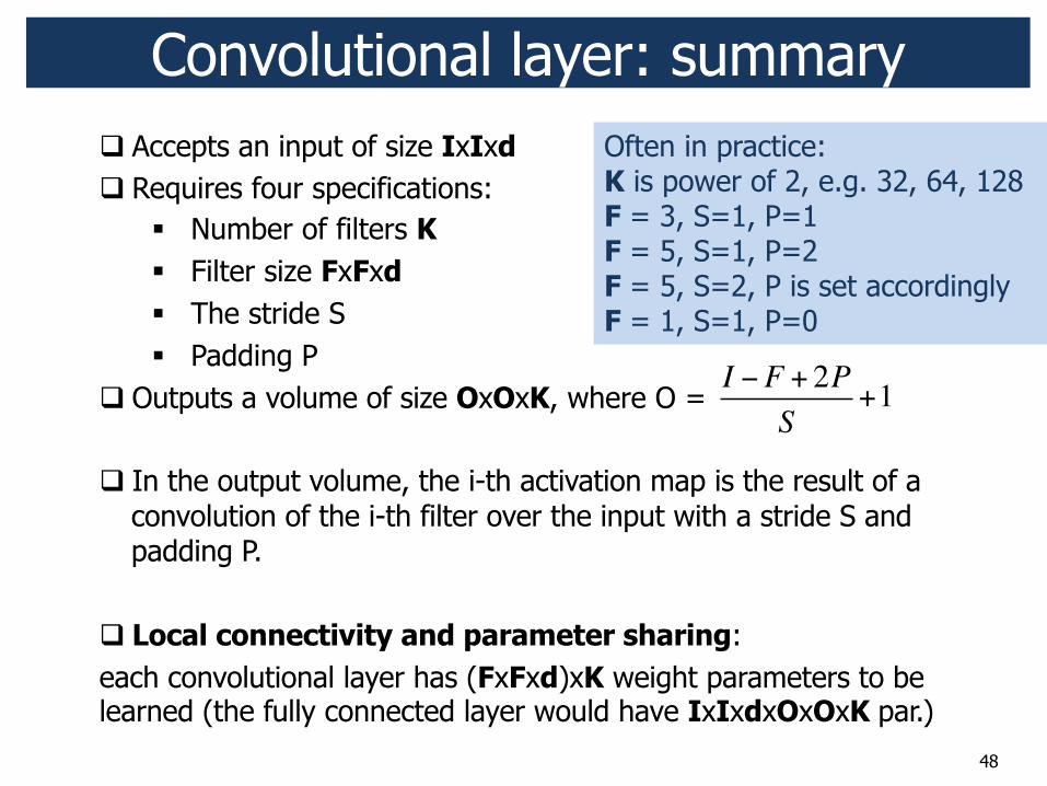
Convolutional layer: summary ! Accepts an input of size IxIxd ! Requires four specifications:
" Number of filters K " Filter size FxFxd " The stride S " Padding P
! Outputs a volume of size OxOxK, where O =
! In the output volume, the i-th activation map is the result of a convolution of the i-th filter over the input with a stride S and padding P.
! Local connectivity and parameter sharing: each convolutional layer has (FxFxd)xK weight parameters to be learned (the fully connected layer would have IxIxdxOxOxK par.)
I !F + 2PS
+1
Often in practice: K is power of 2, e.g. 32, 64, 128 F = 3, S=1, P=1 F = 5, S=1, P=2 F = 5, S=2, P is set accordingly F = 1, S=1, P=0

49
[Convolutional layer: extra]
! We call the layer convolutional because it is related to convolution of two signals:
f [x, y]!g[x, y]= f [n1,n2 ]" g[x # n1, y# n2 ]n2=#$
$
%n1=#$
$
%
elementwise multiplication and sum of a filter and the signal (image)

50
Deep Convolutional Networks
! Convolutional layer ! Non-linear activation function ReLU ! Max pooling layer ! Fully connected layer
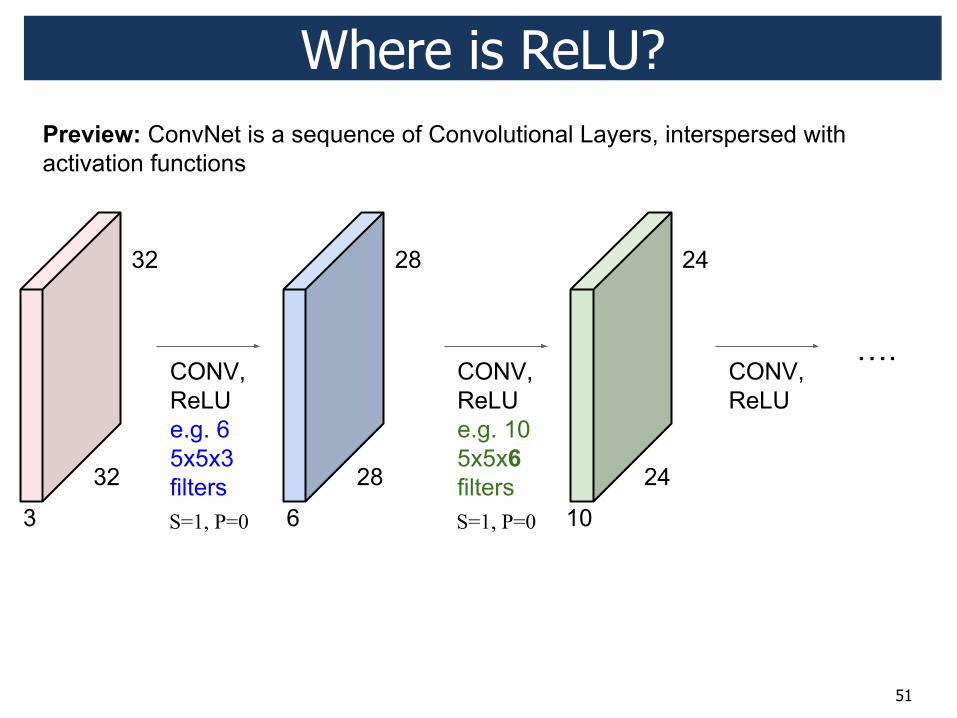
51
Where is ReLU?
S=1, P=0 S=1, P=0
52
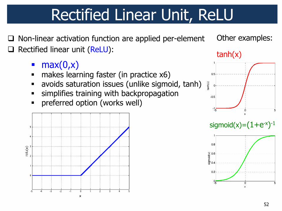
Rectified Linear Unit, ReLU ! Non-linear activation function are applied per-element ! Rectified linear unit (ReLU):
2. Non-Linearity
• Per-element (independent) • Options:
• Tanh • Sigmoid: 1/(1+exp(-x)) • Rectified linear unit (ReLU)
– Simplifies backpropagation – Makes learning faster – Avoids saturation issues – Preferred option (works well)
Rob Fergus
26
Other examples:
" max(0,x) " makes learning faster (in practice x6) " avoids saturation issues (unlike sigmoid, tanh) " simplifies training with backpropagation " preferred option (works well)
sigmoid(x)=(1+e-x)-1
tanh(x)
53
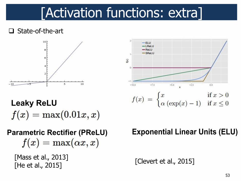
[Activation functions: extra]
[Mass et al., 2013] [He et al., 2015] [Clevert et al., 2015]
! State-of-the-art
54
Deep Convolutional Networks
! Convolutional layer ! Non-linear activation function ReLU ! Max pooling layer ! Fully connected layer
55
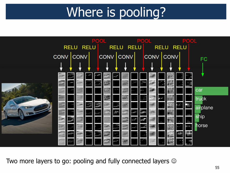
Where is pooling?
Two more layers to go: pooling and fully connected layers #

56
Spatial pooling ! Pooling layer:
! Makes the representations smaller (downsampling) ! Operates over each activation map independently ! Role: invariance to small transformation
57
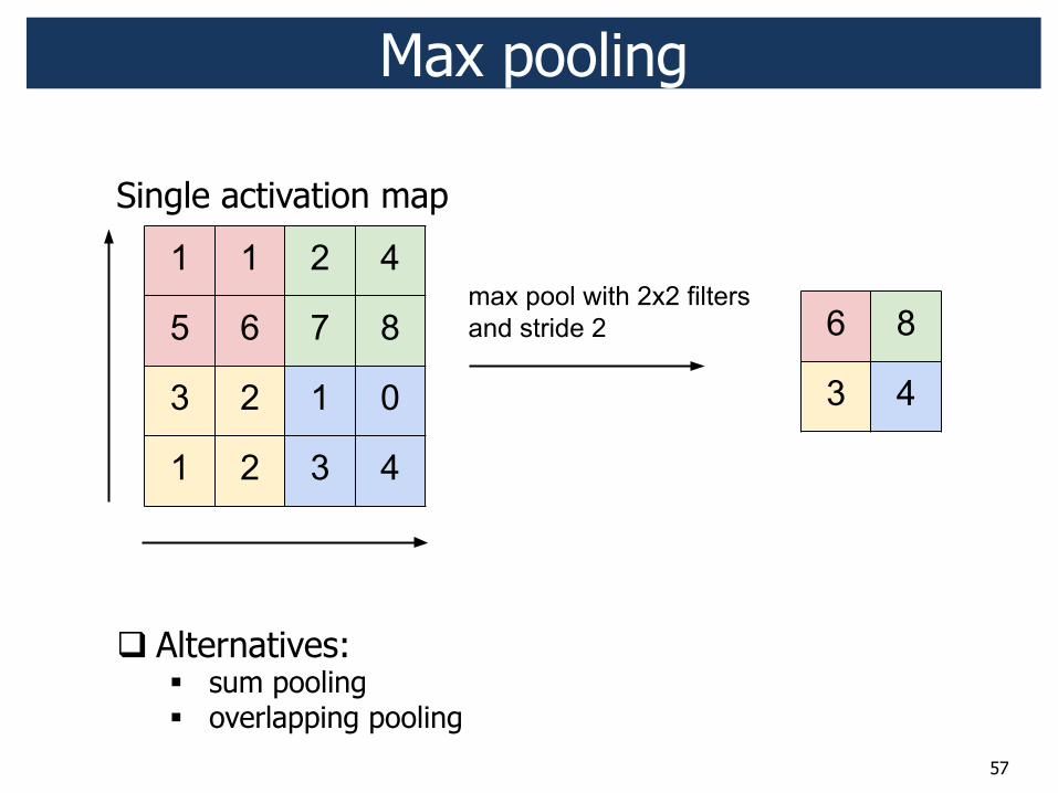
Max pooling
! Alternatives: " sum pooling " overlapping pooling
Single activation map

58
Deep Convolutional Networks
! Convolutional layer ! Non-linear activation function ReLU ! Max pooling layer ! Fully connected layer
59
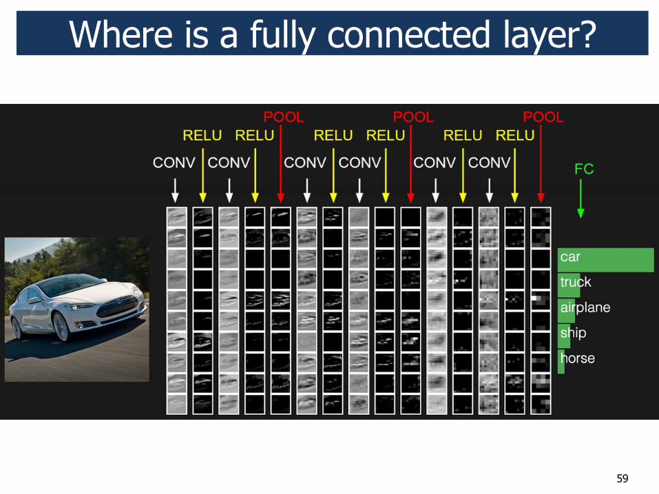
Where is a fully connected layer?
60
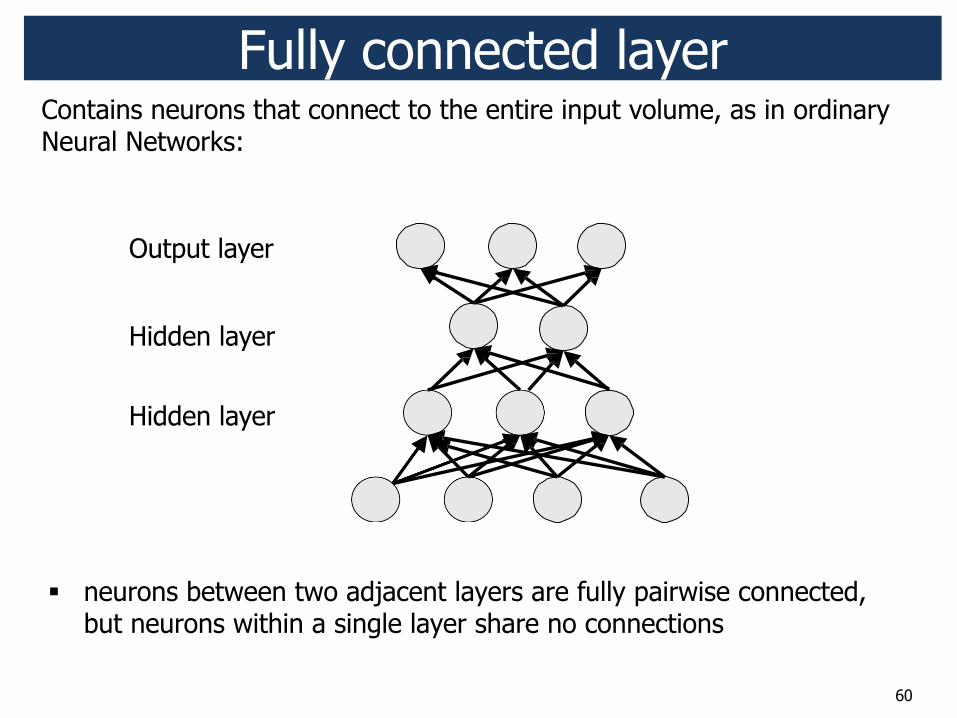
Fully connected layer Contains neurons that connect to the entire input volume, as in ordinary Neural Networks:
Output layer
Hidden layer
" neurons between two adjacent layers are fully pairwise connected, but neurons within a single layer share no connections
Hidden layer
61
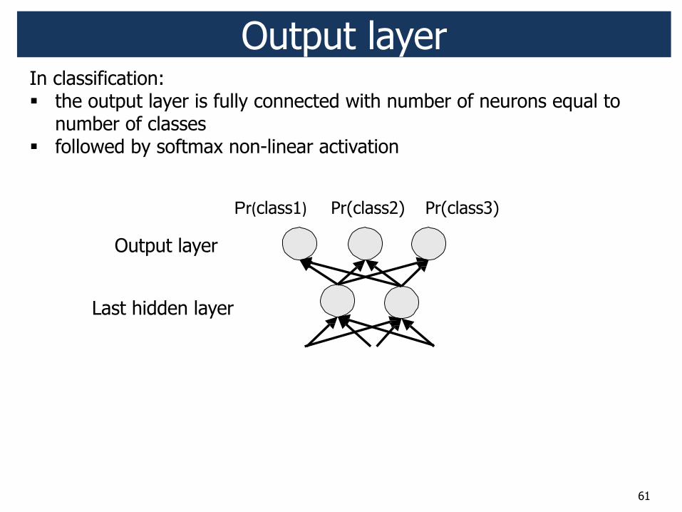
Output layer In classification: " the output layer is fully connected with number of neurons equal to
number of classes " followed by softmax non-linear activation
Output layer
Last hidden layer
Pr<class1=; Pr(class2) Pr(class3)
62
!"#$%%&','/3+>2?7,470%#42#:4%@3?#3/!A%&2+5+4/B'%7482%&.>3?*C,!/8:;
[Running CNNs demo: extra]
63
Case study: AlexNet, 2012
Krizhevsky A, Sutskever I, Hinton G: ImageNet Classification with Deep Convolutional Neural Networks, NIPS 2012
! AlexNet architecture
! Fast-forward to today: Revolution of Depth
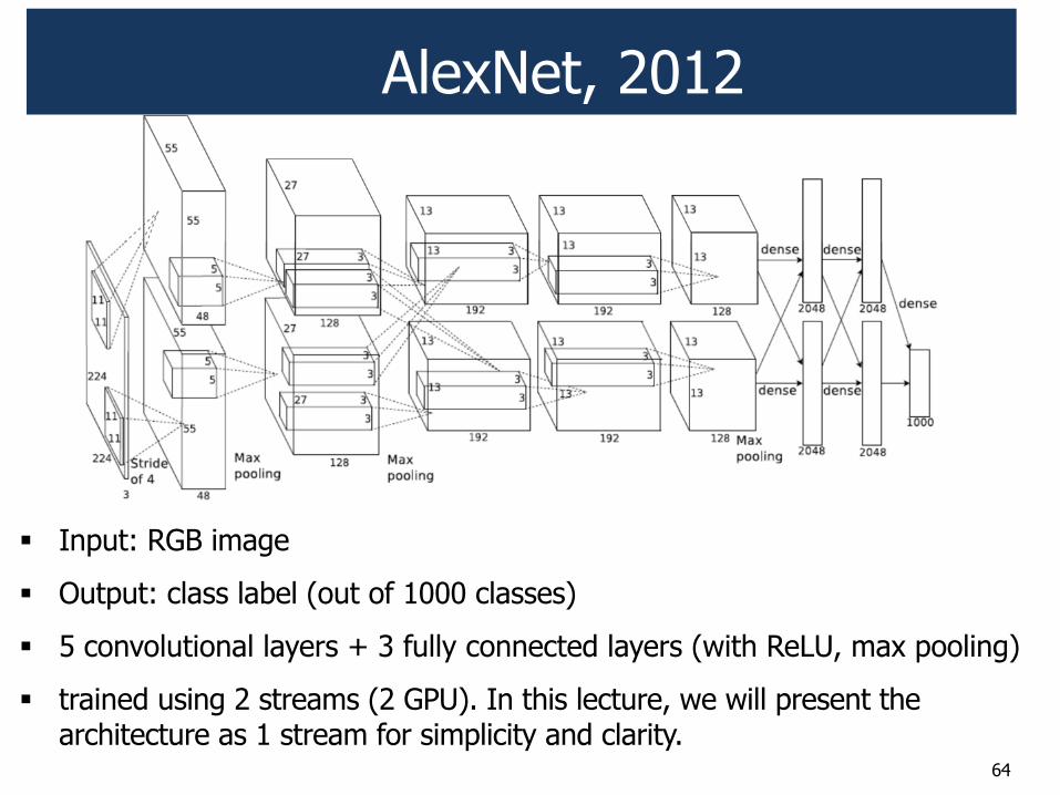
AlexNet, 2012
64
" Input: RGB image
" Output: class label (out of 1000 classes)
" 5 convolutional layers + 3 fully connected layers (with ReLU, max pooling)
" trained using 2 streams (2 GPU). In this lecture, we will present the architecture as 1 stream for simplicity and clarity.
AlexNet, Layer 1
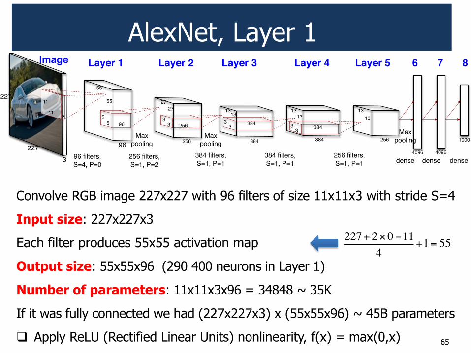
Convolve RGB image 227x227 with 96 filters of size 11x11x3 with stride S=4
Input size: 227x227x3
Each filter produces 55x55 activation map
Output size: 55x55x96 (290 400 neurons in Layer 1)
Number of parameters: 11x11x3x96 = 34848 ~ 35K
If it was fully connected we had (227x227x3) x (55x55x96) ~ 45B parameters
! Apply ReLU (Rectified Linear Units) nonlinearity, f(x) = max(0,x)
227+ 2!0"114
+1= 55
96 256 384 384 256
4096 4096
1000
965
5 2563
3 38433
1313
1313
38433
1313
2727
55
55
Image Layer 1 Layer 4Layer 2 Layer 3 Layer 5 6 7 8
227
2273
3
11
11
96 filters, S=4, P=0
256 filters, S=1, P=2
Max pooling
Max pooling
384 filters, S=1, P=1
384 filters, S=1, P=1
256 filters, S=1, P=1
Max pooling
densedense dense
65

! Max pooling operation (subsampling) along the spatial dimensions
apply with 3x3 filter, stride S=2, padding P=0
Input size: 55x55x96
Output size: 27x27x96 55+ 2!0"3
2+1= 27
AlexNet, Layer 1
66
96 256 384 384 256
4096 4096
1000
965
5 2563
3 38433
1313
1313
38433
1313
2727
55
55
Image Layer 1 Layer 4Layer 2 Layer 3 Layer 5 6 7 8
227
2273
3
11
11
96 filters, S=4, P=0
256 filters, S=1, P=2
Max pooling
Max pooling
384 filters, S=1, P=1
384 filters, S=1, P=1
256 filters, S=1, P=1
Max pooling
densedense dense

AlexNet, Layer 2
Convolve Layer 1 with 256 filters of size 5x5x96 with stride 1, padding 2
Input size: 27x27x96 (after max pooling)
Each filter produces 27x27 activation map
Output size: 27x27x256 (186 624 neurons in Layer 2)
Number of parameters: 5x5x96x256 = 614400 ~ 614K
If it was fully connected we had (27x27x96) x (27x27x256) ~ 13B parameters
! Apply ReLU (Rectified Linear Units) nonlinearity, f(x) = max(0,x)
27+ 2!2" 51
+1= 27
67
96 256 384 384 256
4096 4096
1000
965
5 2563
3 38433
1313
1313
38433
1313
2727
55
55
Image Layer 1 Layer 4Layer 2 Layer 3 Layer 5 6 7 8
227
2273
3
11
11
96 filters, S=4, P=0
256 filters, S=1, P=2
Max pooling
Max pooling
384 filters, S=1, P=1
384 filters, S=1, P=1
256 filters, S=1, P=1
Max pooling
densedense dense

AlexNet, Layer 2
! Max pooling operation (subsampling) along the spatial dimensions
apply with 3x3 filter, stride S=2, padding P=0
Input size: 27x27x256
Output size: 13x13x256 27+ 2!0"3
2+1=13
AlexNet, Layer 2
68
96 256 384 384 256
4096 4096
1000
965
5 2563
3 38433
1313
1313
38433
1313
2727
55
55
Image Layer 1 Layer 4Layer 2 Layer 3 Layer 5 6 7 8
227
2273
3
11
11
96 filters, S=4, P=0
256 filters, S=1, P=2
Max pooling
Max pooling
384 filters, S=1, P=1
384 filters, S=1, P=1
256 filters, S=1, P=1
Max pooling
densedense dense
AlexNet, Layer 3
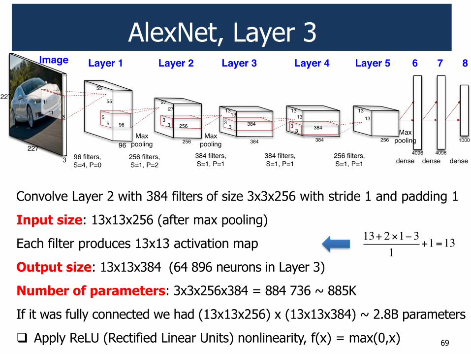
Convolve Layer 2 with 384 filters of size 3x3x256 with stride 1 and padding 1
Input size: 13x13x256 (after max pooling)
Each filter produces 13x13 activation map
Output size: 13x13x384 (64 896 neurons in Layer 3)
Number of parameters: 3x3x256x384 = 884 736 ~ 885K
If it was fully connected we had (13x13x256) x (13x13x384) ~ 2.8B parameters
! Apply ReLU (Rectified Linear Units) nonlinearity, f(x) = max(0,x)
13+ 2!1"31
+1=13
69
96 256 384 384 256
4096 4096
1000
965
5 2563
3 38433
1313
1313
38433
1313
2727
55
55
Image Layer 1 Layer 4Layer 2 Layer 3 Layer 5 6 7 8
227
2273
3
11
11
96 filters, S=4, P=0
256 filters, S=1, P=2
Max pooling
Max pooling
384 filters, S=1, P=1
384 filters, S=1, P=1
256 filters, S=1, P=1
Max pooling
densedense dense

AlexNet, Layer 4
Convolve Layer 3 with 384 filters of size 3x3x384 with stride 1 and padding 1
Input size: 13x13x384
Each filter produces 13x13 activation map
Output size: 13x13x384 (64 896 neurons in Layer 4)
Number of parameters: 3x3x384x384 = 1 327 104~ 1.3M
If it was fully connected we had (13x13x384) x (13x13x384) ~ 4B parameters
! Apply ReLU (Rectified Linear Units) nonlinearity, f(x) = max(0,x)
13+ 2!1"31
+1=13
70
96 256 384 384 256
4096 4096
1000
965
5 2563
3 38433
1313
1313
38433
1313
2727
55
55
Image Layer 1 Layer 4Layer 2 Layer 3 Layer 5 6 7 8
227
2273
3
11
11
96 filters, S=4, P=0
256 filters, S=1, P=2
Max pooling
Max pooling
384 filters, S=1, P=1
384 filters, S=1, P=1
256 filters, S=1, P=1
Max pooling
densedense dense
AlexNet, Layer 5
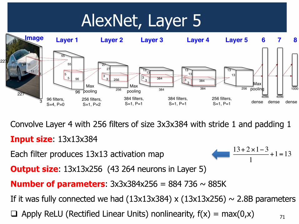
Convolve Layer 4 with 256 filters of size 3x3x384 with stride 1 and padding 1
Input size: 13x13x384
Each filter produces 13x13 activation map
Output size: 13x13x256 (43 264 neurons in Layer 5)
Number of parameters: 3x3x384x256 = 884 736 ~ 885K
If it was fully connected we had (13x13x384) x (13x13x256) ~ 2.8B parameters
! Apply ReLU (Rectified Linear Units) nonlinearity, f(x) = max(0,x)
13+ 2!1"31
+1=13
71
96 256 384 384 256
4096 4096
1000
965
5 2563
3 38433
1313
1313
38433
1313
2727
55
55
Image Layer 1 Layer 4Layer 2 Layer 3 Layer 5 6 7 8
227
2273
3
11
11
96 filters, S=4, P=0
256 filters, S=1, P=2
Max pooling
Max pooling
384 filters, S=1, P=1
384 filters, S=1, P=1
256 filters, S=1, P=1
Max pooling
densedense dense
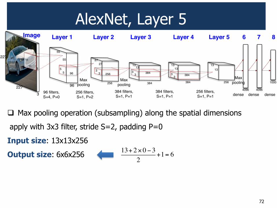
! Max pooling operation (subsampling) along the spatial dimensions
apply with 3x3 filter, stride S=2, padding P=0
Input size: 13x13x256
Output size: 6x6x256 13+ 2!0"3
2+1= 6
AlexNet, Layer 5
72
96 256 384 384 256
4096 4096
1000
965
5 2563
3 38433
1313
1313
38433
1313
2727
55
55
Image Layer 1 Layer 4Layer 2 Layer 3 Layer 5 6 7 8
227
2273
3
11
11
96 filters, S=4, P=0
256 filters, S=1, P=2
Max pooling
Max pooling
384 filters, S=1, P=1
384 filters, S=1, P=1
256 filters, S=1, P=1
Max pooling
densedense dense
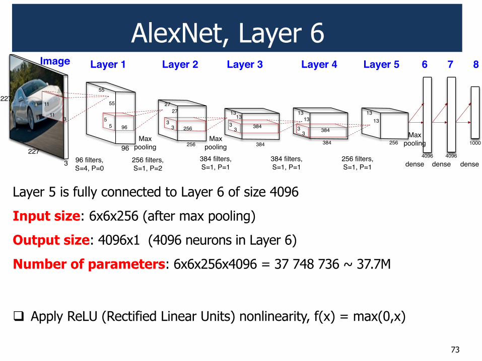
AlexNet, Layer 6
Layer 5 is fully connected to Layer 6 of size 4096
Input size: 6x6x256 (after max pooling)
Output size: 4096x1 (4096 neurons in Layer 6)
Number of parameters: 6x6x256x4096 = 37 748 736 ~ 37.7M
! Apply ReLU (Rectified Linear Units) nonlinearity, f(x) = max(0,x)
73
96 256 384 384 256
4096 4096
1000
965
5 2563
3 38433
1313
1313
38433
1313
2727
55
55
Image Layer 1 Layer 4Layer 2 Layer 3 Layer 5 6 7 8
227
2273
3
11
11
96 filters, S=4, P=0
256 filters, S=1, P=2
Max pooling
Max pooling
384 filters, S=1, P=1
384 filters, S=1, P=1
256 filters, S=1, P=1
Max pooling
densedense dense
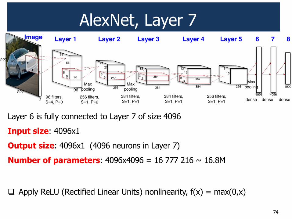
AlexNet, Layer 7
Layer 6 is fully connected to Layer 7 of size 4096
Input size: 4096x1
Output size: 4096x1 (4096 neurons in Layer 7)
Number of parameters: 4096x4096 = 16 777 216 ~ 16.8M
74
96 256 384 384 256
4096 4096
1000
965
5 2563
3 38433
1313
1313
38433
1313
2727
55
55
Image Layer 1 Layer 4Layer 2 Layer 3 Layer 5 6 7 8
227
2273
3
11
11
96 filters, S=4, P=0
256 filters, S=1, P=2
Max pooling
Max pooling
384 filters, S=1, P=1
384 filters, S=1, P=1
256 filters, S=1, P=1
Max pooling
densedense dense
! Apply ReLU (Rectified Linear Units) nonlinearity, f(x) = max(0,x)

AlexNet, Layer 8
Layer 7 is fully connected to Layer 8 of size 1000
Input size: 4096x1
Output size: 1000x1 (1000 neurons in Layer 8)
Number of parameters: 4096x1000 = 4 096 000~ 4M
Apply: softmax non-linear activation to obtain probability scores for 1000 classes
Pr(class = i | x1, x2,..., x1000 ) = exp(xi ) / exp(xk )k=1
1000
!75
96 256 384 384 256
4096 4096
1000
965
5 2563
3 38433
1313
1313
38433
1313
2727
55
55
Image Layer 1 Layer 4Layer 2 Layer 3 Layer 5 6 7 8
227
2273
3
11
11
96 filters, S=4, P=0
256 filters, S=1, P=2
Max pooling
Max pooling
384 filters, S=1, P=1
384 filters, S=1, P=1
256 filters, S=1, P=1
Max pooling
densedense dense
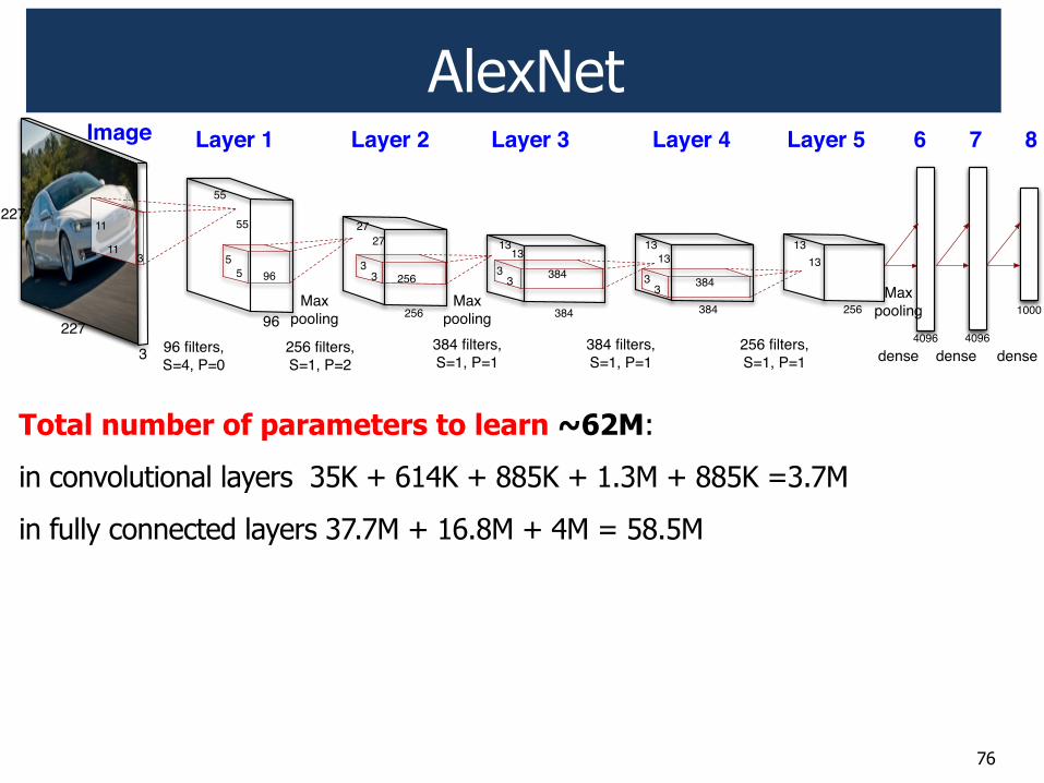
AlexNet
Total number of parameters to learn ~62M:
in convolutional layers 35K + 614K + 885K + 1.3M + 885K =3.7M
in fully connected layers 37.7M + 16.8M + 4M = 58.5M
76
96 256 384 384 256
4096 4096
1000
965
5 2563
3 38433
1313
1313
38433
1313
2727
55
55
Image Layer 1 Layer 4Layer 2 Layer 3 Layer 5 6 7 8
227
2273
3
11
11
96 filters, S=4, P=0
256 filters, S=1, P=2
Max pooling
Max pooling
384 filters, S=1, P=1
384 filters, S=1, P=1
256 filters, S=1, P=1
Max pooling
densedense dense
77
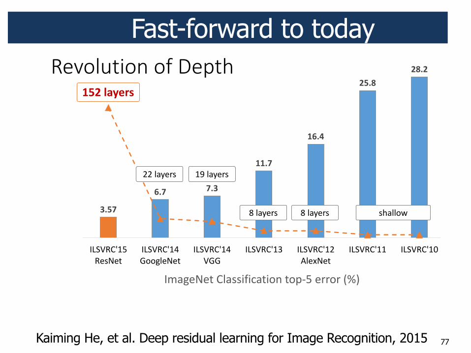
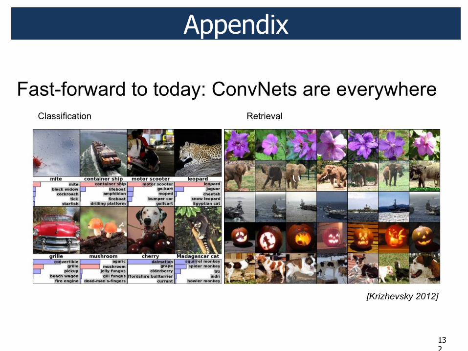
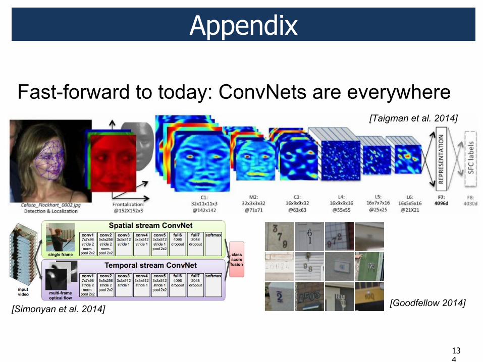
Fast-forward to today
Kaiming He, et al. Deep residual learning for Image Recognition, 2015
!"#$%&'($)*$+*,"-'.
!"#$
%"$ $"!
&&"$
&%"'
(#")()"(
!"#$%&'()%*+,*-
!"#$%&'(./0012*,*-
!"#$%&'(.$//
!"#$%&'(3 !"#$%&'(452*6,*-
!"#$%&'(( !"#$%&'(7
!891*,*-:&29++;<;=9-;0>:-0?@):*AA0A:BCD
+E9220FG:29H*A+
(I:29H*A+44:29H*A+
&#(*+,-./0
J9;8;>1:K*L:M;9>1HN:OE9>1L:#E90P;>1:%*>L:Q:R;9>:#N>S:TU**?:%*+;VN92:"*9A>;>1:<0A:!891*:%*=01>;-;0>WS:9AM;X:47()S
G:29H*A+
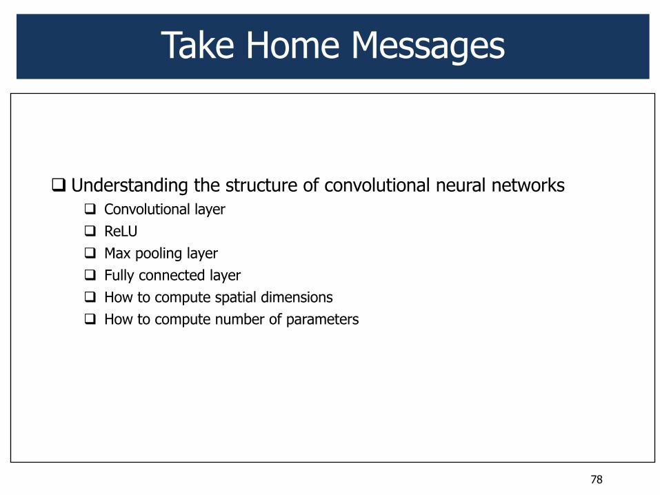
! Understanding the structure of convolutional neural networks
! Convolutional layer ! ReLU ! Max pooling layer ! Fully connected layer ! How to compute spatial dimensions ! How to compute number of parameters
78
Take Home Messages
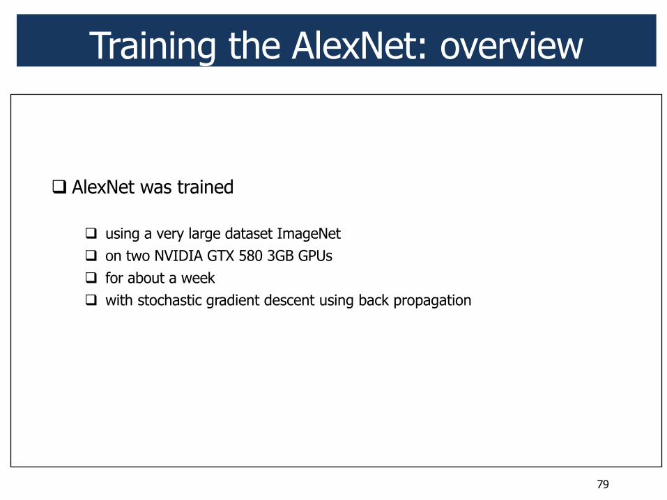
! AlexNet was trained
! using a very large dataset ImageNet ! on two NVIDIA GTX 580 3GB GPUs ! for about a week ! with stochastic gradient descent using back propagation
79
Training the AlexNet: overview
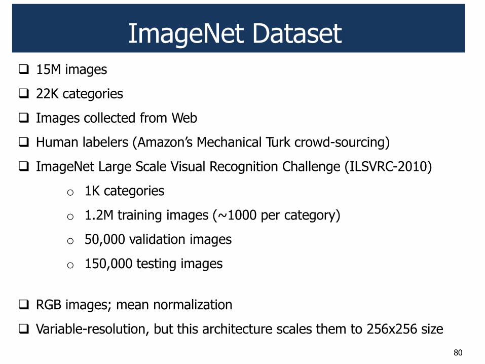
! 15M images
! 22K categories
! Images collected from Web
! Human labelers (Amazon’s Mechanical Turk crowd-sourcing)
! ImageNet Large Scale Visual Recognition Challenge (ILSVRC-2010)
o 1K categories
o 1.2M training images (~1000 per category)
o 50,000 validation images
o 150,000 testing images
! RGB images; mean normalization
! Variable-resolution, but this architecture scales them to 256x256 size
ImageNet Dataset
80
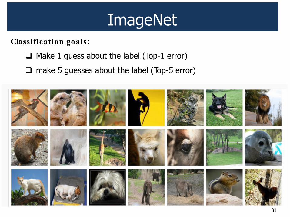
Classification goals :
! Make 1 guess about the label (Top-1 error)
! make 5 guesses about the label (Top-5 error)
ImageNet
81
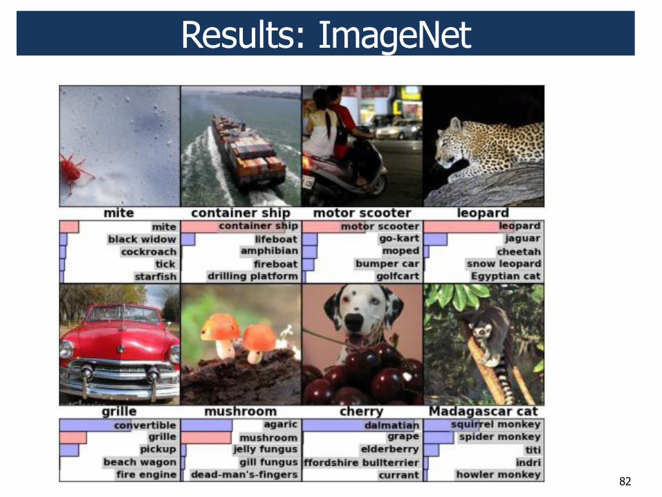
Results: ImageNet
82
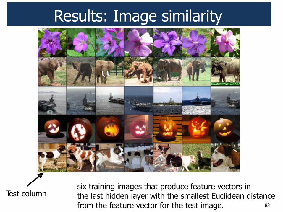
Results: Image similarity
Test column six training images that produce feature vectors in the last hidden layer with the smallest Euclidean distance from the feature vector for the test image. 83

Deep Learning, Part 2
G6032, G6061, 934G5, 807G5, G5015
Dr. Viktoriia Sharmanska
Content
! Training Deep Convolutional Neural Networks
! Stochastic gradient descent ! Backpropagation ! Initialization
! Preventing overfitting
! Dropout regularization ! Data augmentation
! Fine-tuning
! Visualization of CNNs
85
86
Training CNNs ! Stochastic gradient descent ! Backpropagation ! Initialization
Stochastic gradient descent (SGD)
87
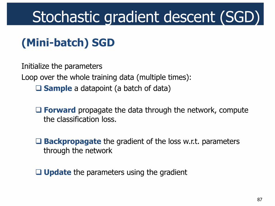
(Mini-batch) SGD Initialize the parameters Loop over the whole training data (multiple times):
! Sample a datapoint (a batch of data) ! Forward propagate the data through the network, compute
the classification loss.
! Backpropagate the gradient of the loss w.r.t. parameters through the network
! Update the parameters using the gradient

Stochastic gradient descent (SGD)
88
(Mini-batch) SGD Initialize the parameters randomly but smartly Loop over the whole training data (multiple times):
! Sample a datapoint (a batch of data) ! Forward propagate the data through the network, compute
the classification loss. For example:
! Backpropagate the gradient of the loss w.r.t. parameters through the network
! Update the parameters using the gradient
SGD:
E = 12(ypredicted ! ytrue )
2
wt+1 = wt !! "dEdw(wt )
Backpropagation
89
! Backpropagation is recursive application of the chain rule along a computational flow of the network to compute gradients of the loss function w.r.t. all parameters/intermediate variables/inputs in the network
Backpropagation
90
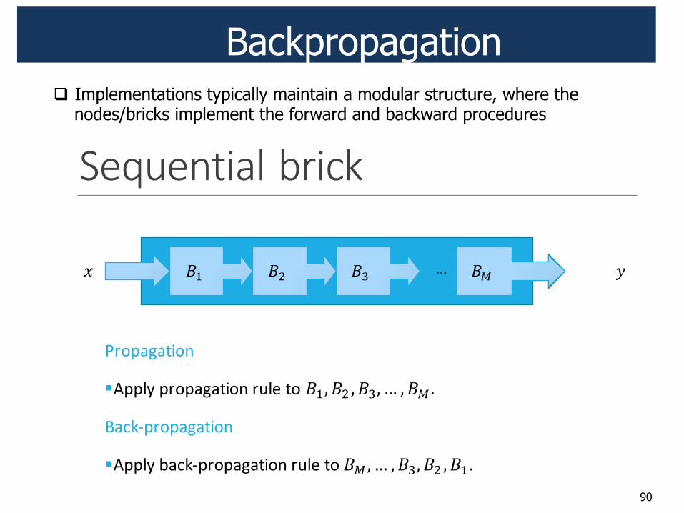
! Implementations typically maintain a modular structure, where the nodes/bricks implement the forward and backward procedures
!"#$"%&'()*+,'-.
!"#$%&%'(#)
!*$$+,-$"#$%&%'(#)-".+/-'#-!"# !$# !%# & # !'(0%123$"#$%&%'(#)
!*$$+,-4%123$"#$%&%'(#)-".+/-'#-!'#& # !%# !$# !"5
) *!" !$ !% !'6
Backpropagation
91
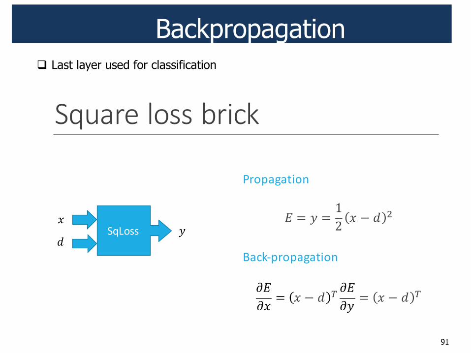
!"#$%&'()**'+%,-.
!"#$%&%'(#)
! " # " $% & ' ( )
*%+,-$"#$%&%'(#)
*!*& " & ' ( + *!
*# " & ' ( +
./0#11&
#(
! Last layer used for classification

Backpropagation
92
!"##$%&'()#
!"#$%&%'(#) *%+,-$"#$%&%'(#)
!"#$%& ! "#
$% & ' $ ()
(*" % & ' + ()
(,
'()* ---------------------------. " /0 ! " 12340 5 678*9()
(*"
78
#:;<=()
(,
+,-)&**************. " /0 ! " >?@4ABC & .%9()
(*" &.--DE.% F CG
()
(,
'()!(./0$1 . " 0HI ! " 123 J 6*KL -&%8()
(* M" 6*N J 6*KLO & PM8
()
(,
0$10$%),-------. " 0 HI ! " >?@LQ8
%L 5 C & %8:
()
(* M" PMLR & PM8 -DES T AG
()
(,
! Typical choices
Backpropagation
93
!"#$%&'(&")*
!"#$%&%'(#)
! " #$
*%+,-$"#$%&%'(#)
%&%$ " '
%&%! #
%&%# " $' %&%!
.()/%"
#
$ !
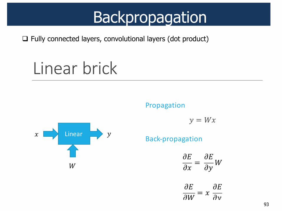
! Fully connected layers, convolutional layers (dot product)
Backpropagation
94
!"#$%&'"(&)$*+,-$(.",*/
!"#$%&%'(#)
!" # $%&"'
*%+,-$"#$%&%'(#)
()(& "
# ()(! "
*$+%&"'
$& !
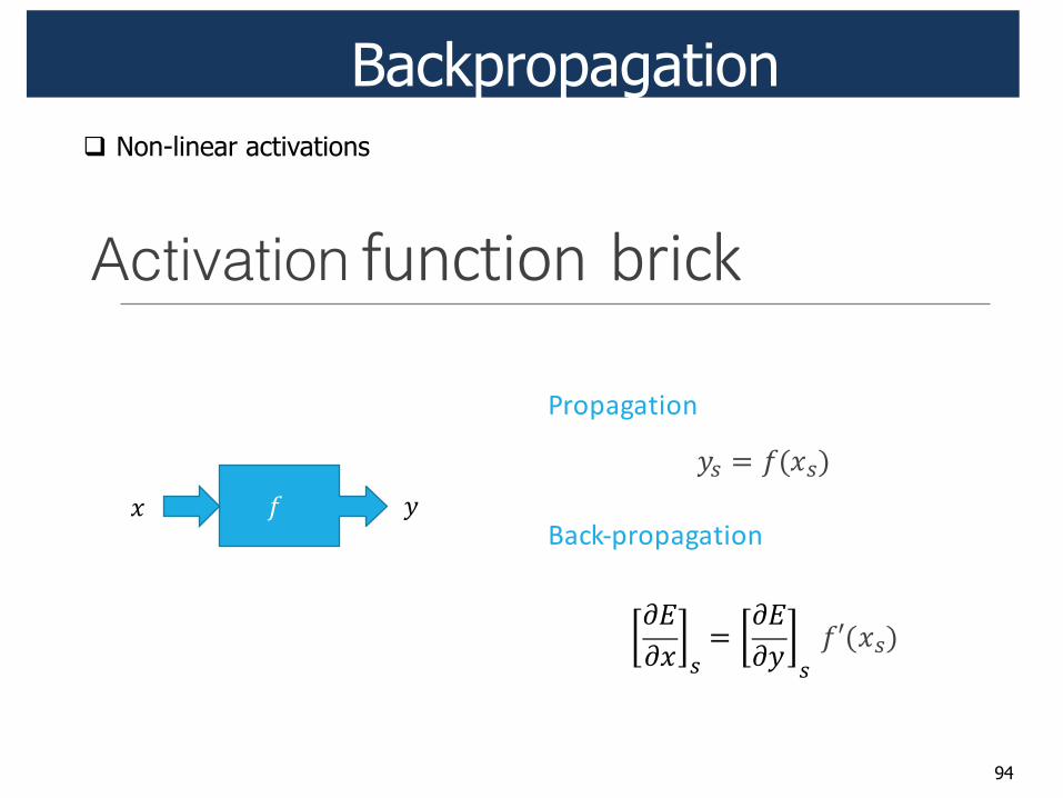
! Non-linear activations
Activation
Backpropagation
95
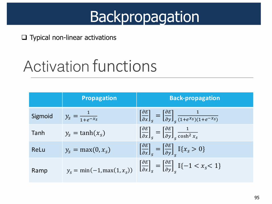
! Typical non-linear activations
!"#$%&'"(&)$*+,-$%
!"#$%&%'(#) *%+,-$"#$%&%'(#)
!"#$%"& !" # $$%&'()
*+*, "
# *+*- "
$.$%&()/.$%&'()/
'()* !" # 01234.5"/*+*, "
# *+*- "
$6789: ,)
+,-. !" # ;1<.=> 5"/*+*, "
# *+*- "
?@5" A =B
+($/ !" # ;C2 DE>;1< E> 5"*+*, "
# *+*- "
?@DE F 5"F EB
Activation

96
Recap: ReLU ! Non-linear activation function are applied per-element ! Rectified linear unit (ReLU):
2. Non-Linearity
• Per-element (independent) • Options:
• Tanh • Sigmoid: 1/(1+exp(-x)) • Rectified linear unit (ReLU)
– Simplifies backpropagation – Makes learning faster – Avoids saturation issues – Preferred option (works well)
Rob Fergus
26
Other examples:
" max(0,x) " makes learning faster (in practice x6) " avoids saturation issues (unlike sigmoid, tanh) " simplifies training with backpropagation " preferred option (works well)
sigmoid(x)=(1+e-x)-1
tanh(x)
97
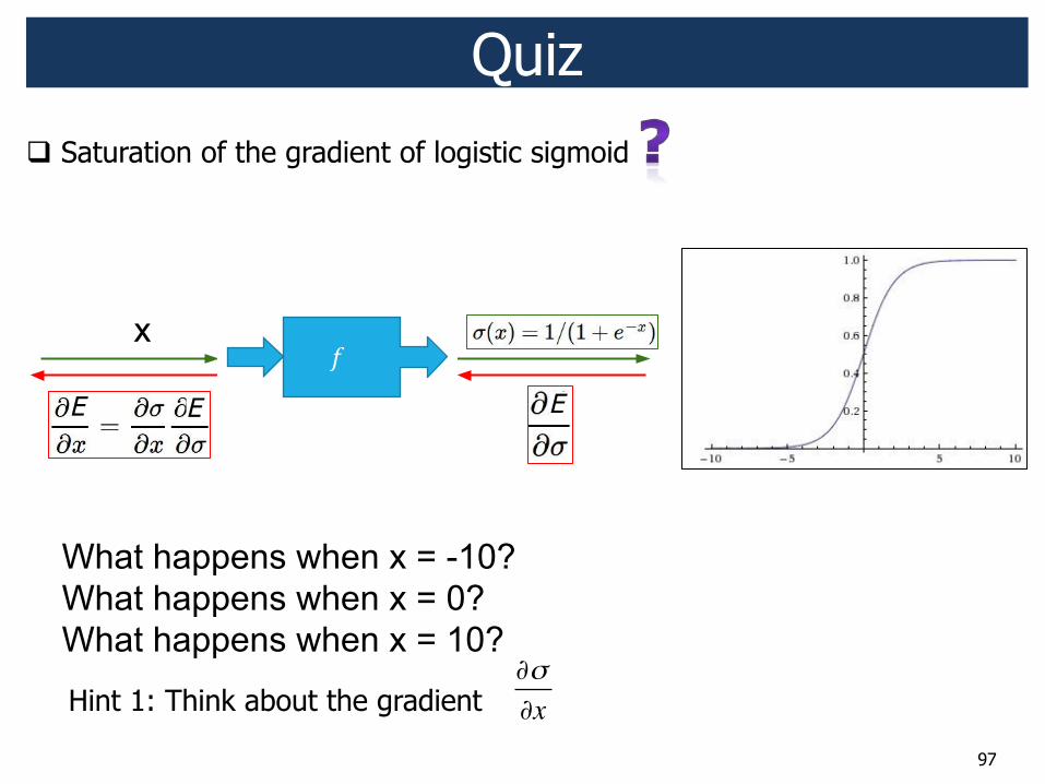
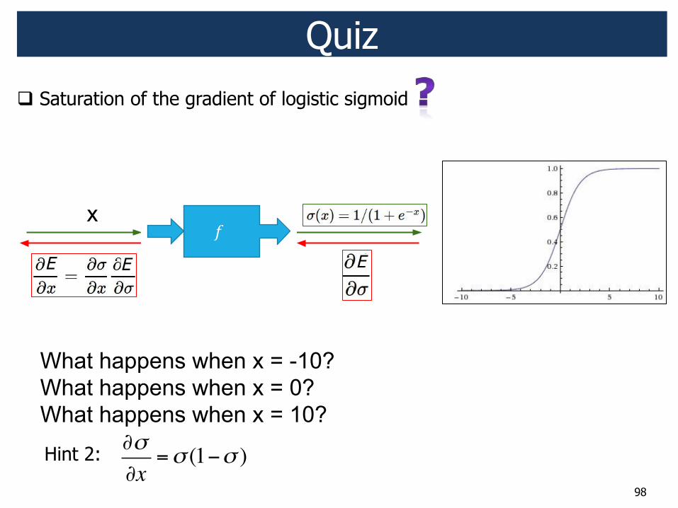
! Saturation of the gradient of logistic sigmoid Quiz
Hint 1: Think about the gradient !!!x
!"#$%&'"(&)$*+,-$(.",*/
!"#$%&%'(#)
!" # $%&"'
*%+,-$"#$%&%'(#)
()(& "
# ()(! "
*$+%&"'
$& !E E E
98
! Saturation of the gradient of logistic sigmoid Quiz
!"#$%&'"(&)$*+,-$(.",*/
!"#$%&%'(#)
!" # $%&"'
*%+,-$"#$%&%'(#)
()(& "
# ()(! "
*$+%&"'
$& !E E E
Hint 2: !!!x
=! (1"! )
99
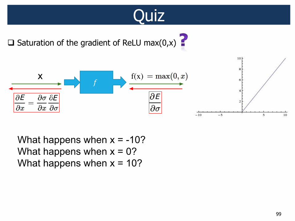
Quiz ! Saturation of the gradient of ReLU max(0,x)
!"#$%&'"(&)$*+,-$(.",*/
!"#$%&%'(#)
!" # $%&"'
*%+,-$"#$%&%'(#)
()(& "
# ()(! "
*$+%&"'
$& !E E E
f(x)!
100
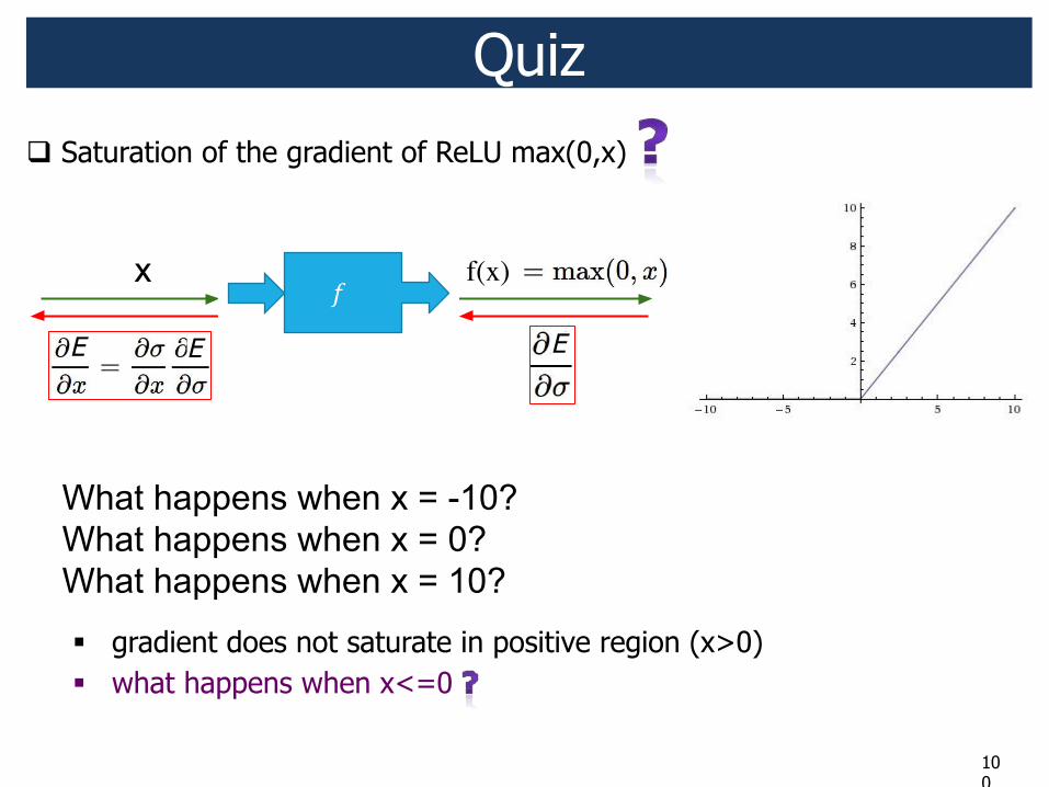
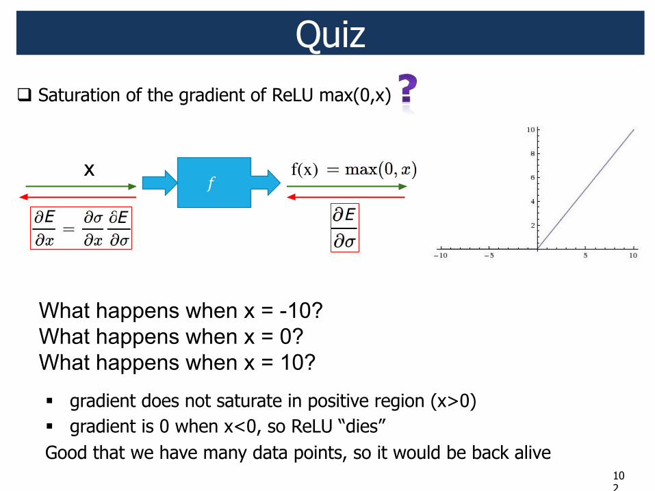
Quiz ! Saturation of the gradient of ReLU max(0,x)
!"#$%&'"(&)$*+,-$(.",*/
!"#$%&%'(#)
!" # $%&"'
*%+,-$"#$%&%'(#)
()(& "
# ()(! "
*$+%&"'
$& !E E E
f(x)!
" gradient does not saturate in positive region (x>0) " what happens when x<=0
101
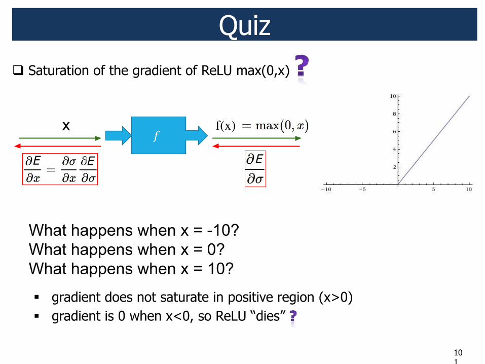
Quiz ! Saturation of the gradient of ReLU max(0,x)
!"#$%&'"(&)$*+,-$(.",*/
!"#$%&%'(#)
!" # $%&"'
*%+,-$"#$%&%'(#)
()(& "
# ()(! "
*$+%&"'
$& !E E E
f(x)!
" gradient does not saturate in positive region (x>0) " gradient is 0 when x<0, so ReLU “dies”
102
Quiz ! Saturation of the gradient of ReLU max(0,x)
!"#$%&'"(&)$*+,-$(.",*/
!"#$%&%'(#)
!" # $%&"'
*%+,-$"#$%&%'(#)
()(& "
# ()(! "
*$+%&"'
$& !E E E
f(x)!
" gradient does not saturate in positive region (x>0) " gradient is 0 when x<0, so ReLU “dies” Good that we have many data points, so it would be back alive
103
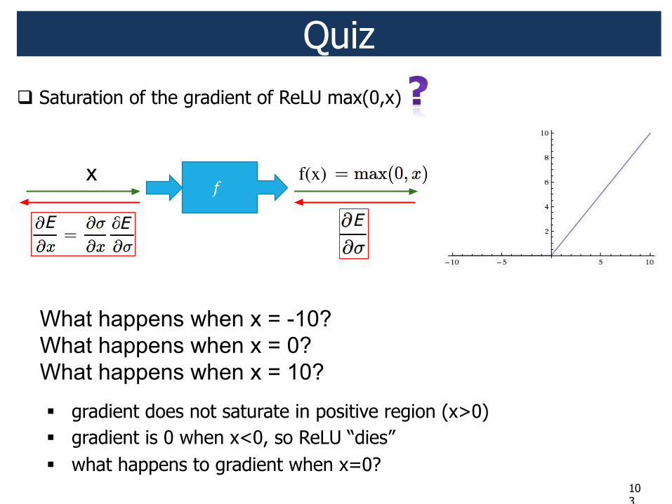
Quiz ! Saturation of the gradient of ReLU max(0,x)
!"#$%&'"(&)$*+,-$(.",*/
!"#$%&%'(#)
!" # $%&"'
*%+,-$"#$%&%'(#)
()(& "
# ()(! "
*$+%&"'
$& !E E E
f(x)!
" gradient does not saturate in positive region (x>0) " gradient is 0 when x<0, so ReLU “dies” " what happens to gradient when x=0?
104
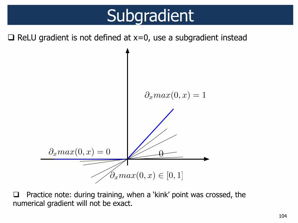
Subgradient
0
∂xmax(0, x) = 1
∂xmax(0, x) = 0
∂xmax(0, x) ∈ [0, 1]
! ReLU gradient is not defined at x=0, use a subgradient instead
! Practice note: during training, when a ‘kink’ point was crossed, the numerical gradient will not be exact.
105
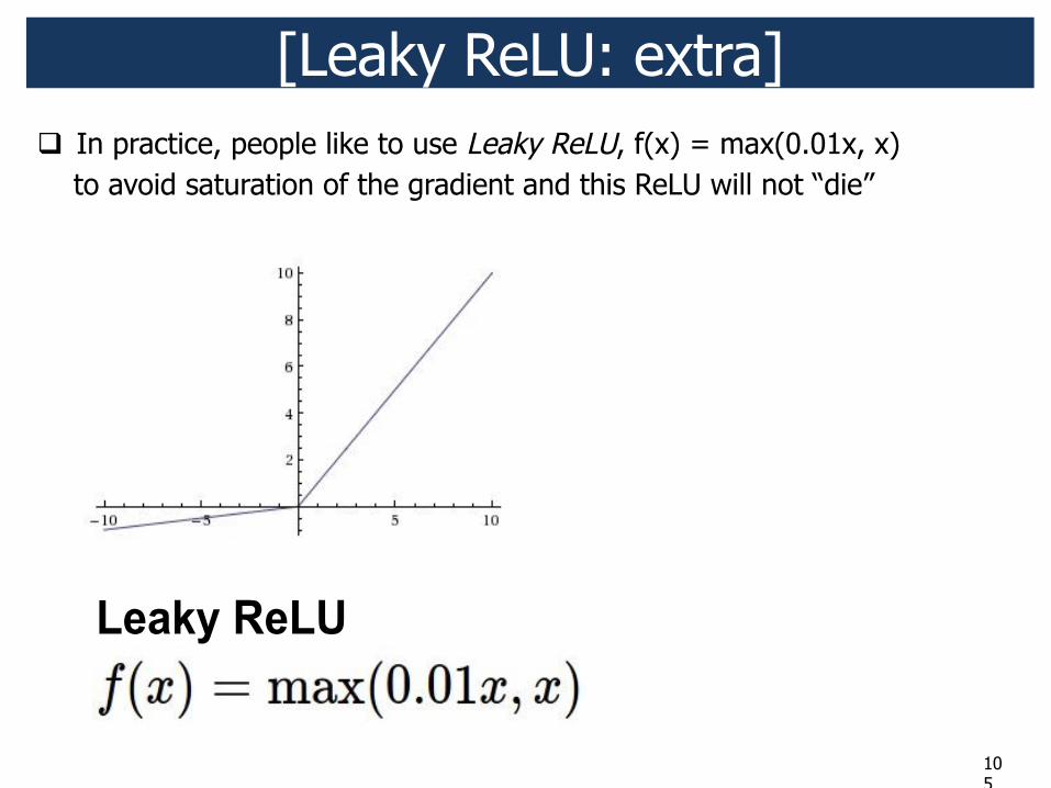
! In practice, people like to use Leaky ReLU, f(x) = max(0.01x, x) to avoid saturation of the gradient and this ReLU will not “die”
[Leaky ReLU: extra]
106
Training CNNs ! Stochastic gradient descent ! Backpropagation ! Initialization
Stochastic gradient descent (SGD)
107
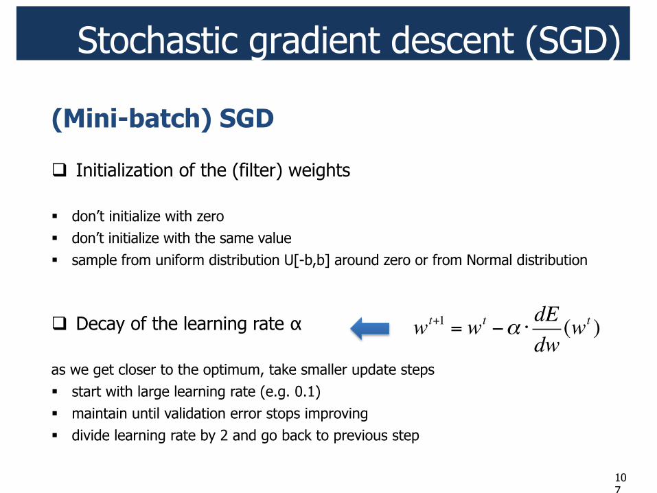
(Mini-batch) SGD
! Initialization of the (filter) weights " don’t initialize with zero " don’t initialize with the same value " sample from uniform distribution U[-b,b] around zero or from Normal distribution
! Decay of the learning rate α as we get closer to the optimum, take smaller update steps " start with large learning rate (e.g. 0.1) " maintain until validation error stops improving " divide learning rate by 2 and go back to previous step
wt+1 = wt !! "dEdw(wt )
Stochastic gradient descent (SGD)
108
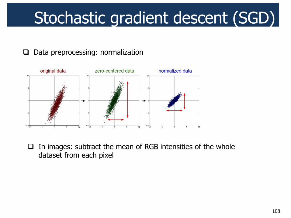
! Data preprocessing: normalization
! In images: subtract the mean of RGB intensities of the whole dataset from each pixel

109
Preventing overfitting ! Dropout regularization ! Data augmentation
110
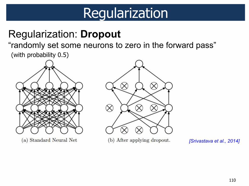
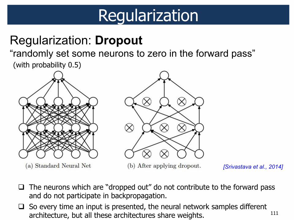
Regularization
(with probability 0.5)
111
Regularization
(with probability 0.5)
! The neurons which are “dropped out” do not contribute to the forward pass and do not participate in backpropagation.
! So every time an input is presented, the neural network samples different architecture, but all these architectures share weights.
112
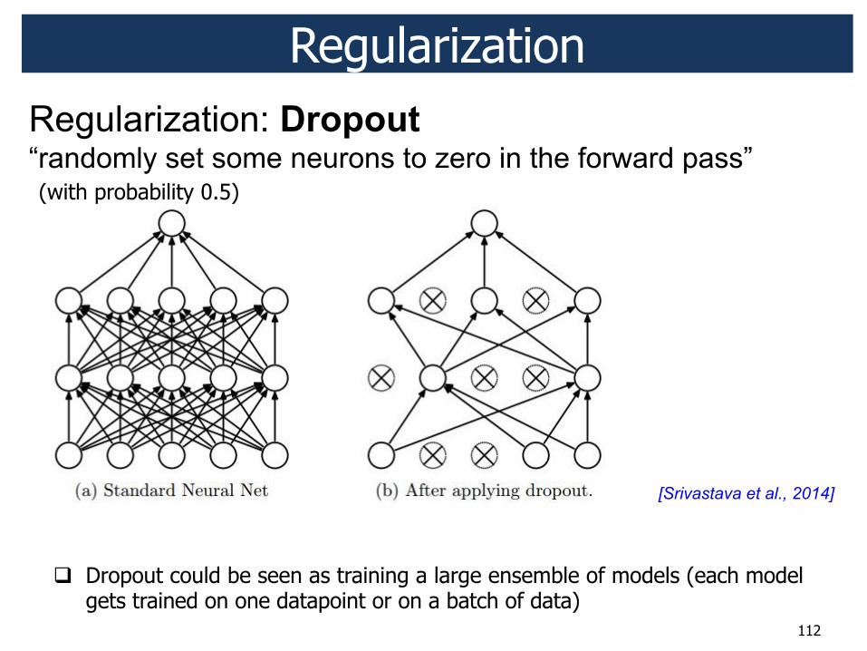
Regularization
! Dropout could be seen as training a large ensemble of models (each model gets trained on one datapoint or on a batch of data)
(with probability 0.5)
113
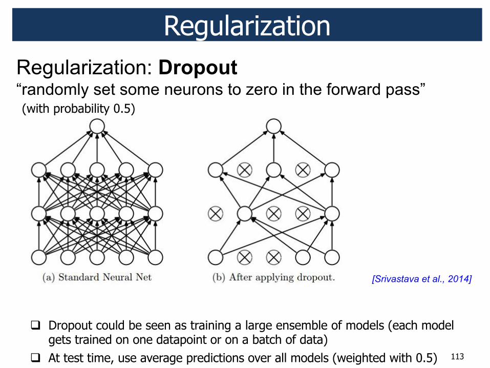
Regularization
! Dropout could be seen as training a large ensemble of models (each model gets trained on one datapoint or on a batch of data)
! At test time, use average predictions over all models (weighted with 0.5)
(with probability 0.5)
Dropout: set the output of each hidden neuron to zero w.p. 0.5.
" This technique reduces complex co-adaptations of neurons, since a neuron cannot rely on the presence of particular other neurons.
" It is, therefore, forced to learn more robust features that are useful in conjunction with many different random subsets of the other neurons.
" Without dropout, CNNs exhibits substantial overfitting.
" Dropout roughly doubles the number of iterations required to converge.
Alternatives:
standard L2 regularization of weights
Dropout
114
Dropout
Data Augmentation
115
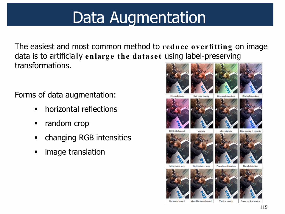
The easiest and most common method to reduce overfitting on image data is to artificially enlarg e the dataset using label-preserving transformations. Forms of data augmentation:
" horizontal reflections
" random crop
" changing RGB intensities
" image translation

116
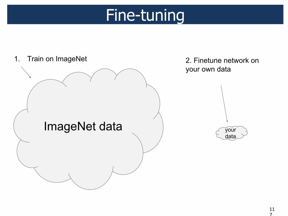
Fine-tuning
117
Fine-tuning
118
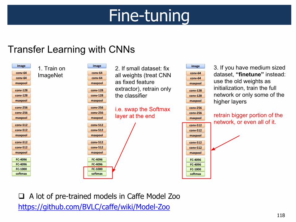
Fine-tuning
! A lot of pre-trained models in Caffe Model Zoo https://github.com/BVLC/caffe/wiki/Model-Zoo
119
Visualization of CNNs
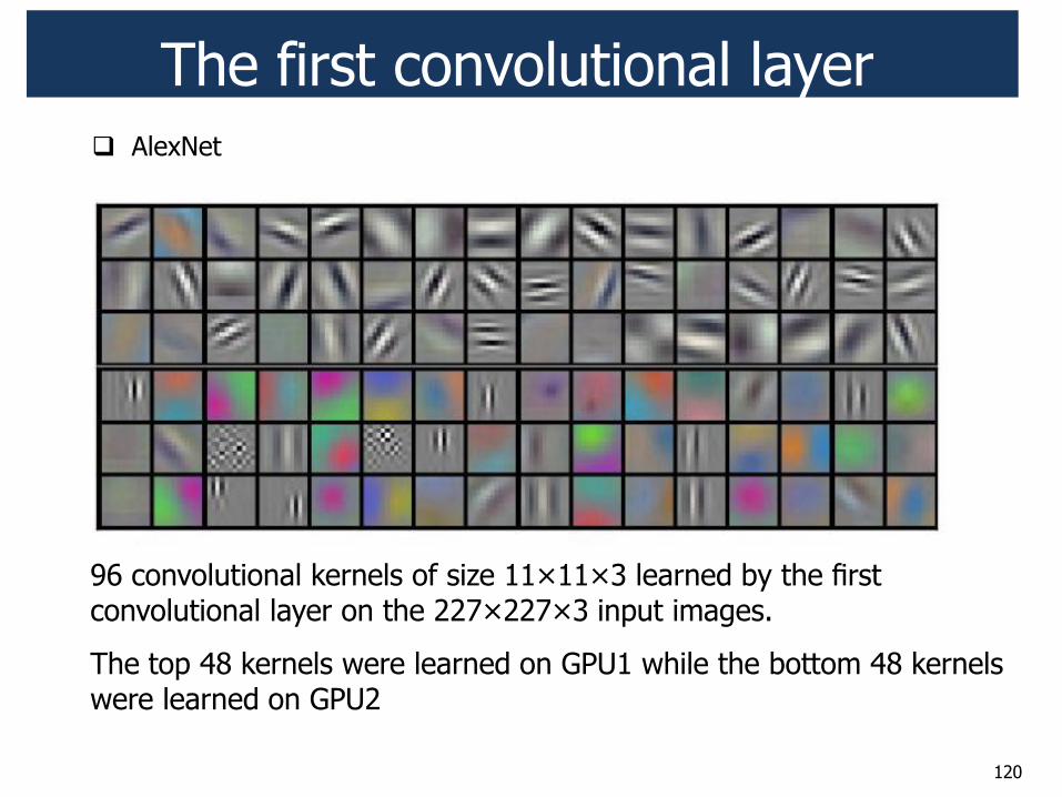
96 convolutional kernels of size 11!11!3 learned by the first convolutional layer on the 227!227!3 input images.
The top 48 kernels were learned on GPU1 while the bottom 48 kernels were learned on GPU2
The first convolutional layer
120
! AlexNet
The first convolutional layer
121
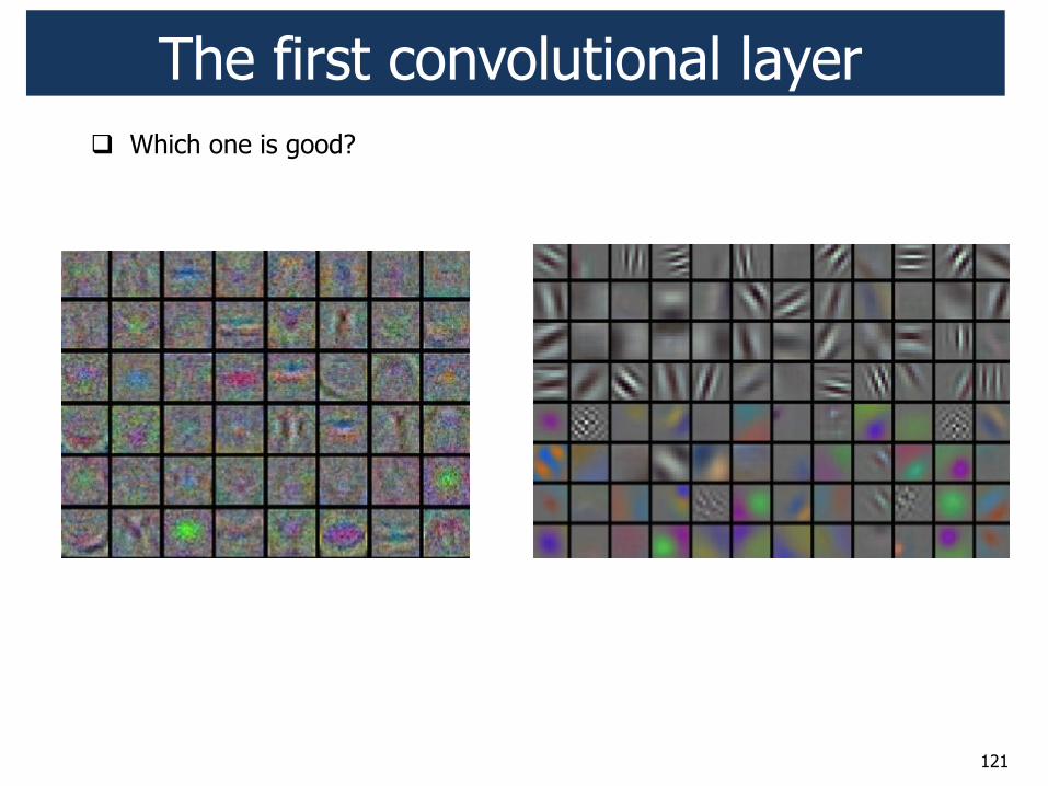
! Which one is good?
The first convolutional layer
122
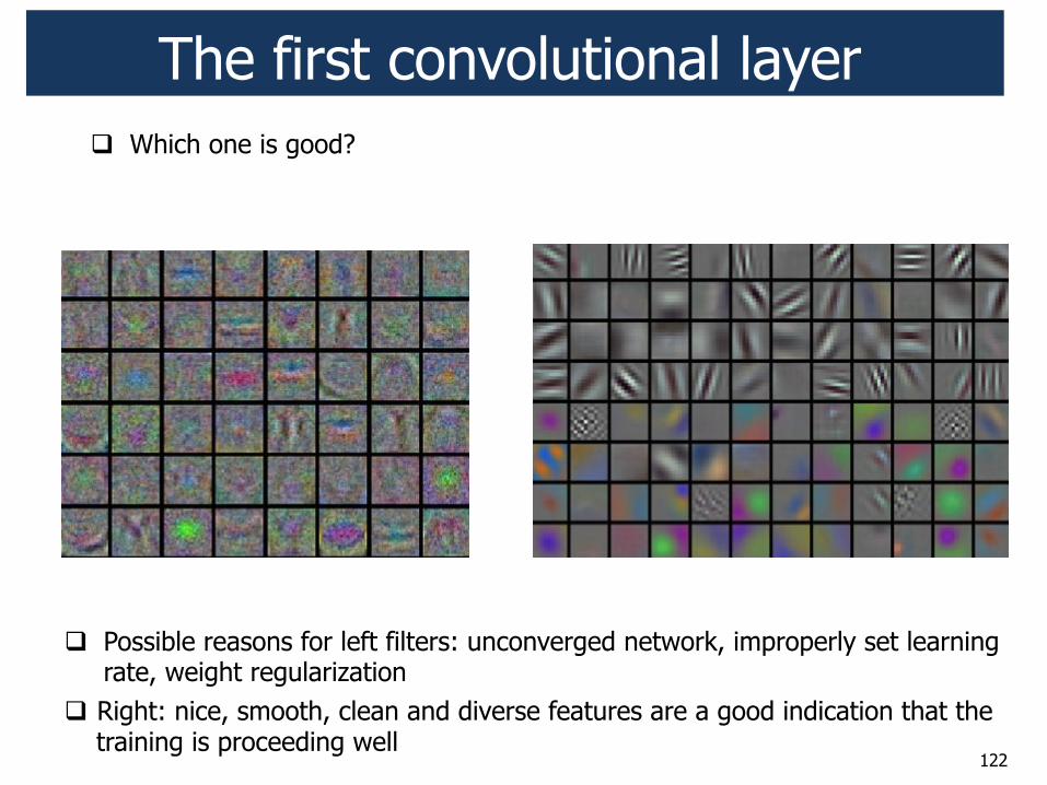
! Which one is good?
! Possible reasons for left filters: unconverged network, improperly set learning rate, weight regularization
! Right: nice, smooth, clean and diverse features are a good indication that the training is proceeding well
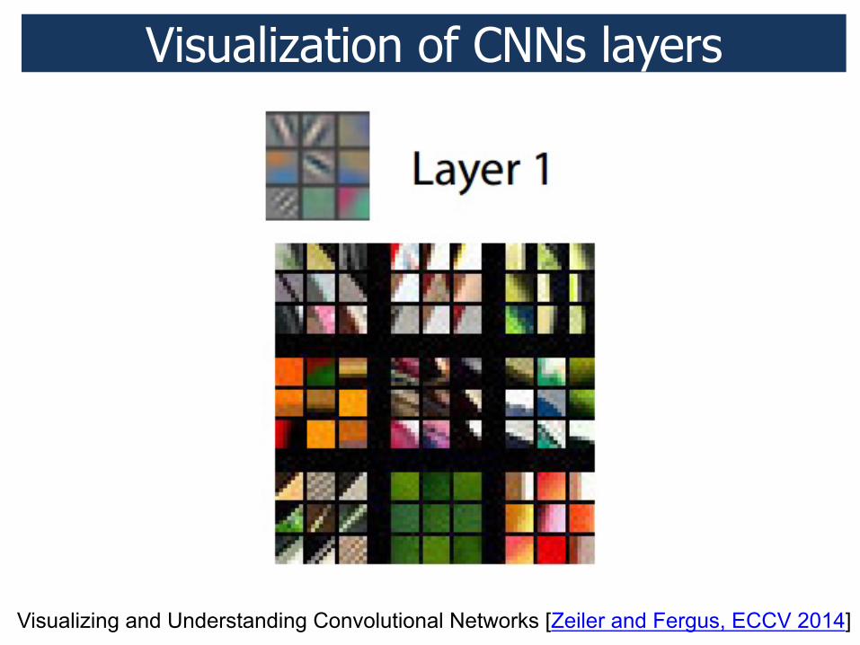
Layer 1
Visualizing and Understanding Convolutional Networks [Zeiler and Fergus, ECCV 2014]
Visualization of CNNs layers
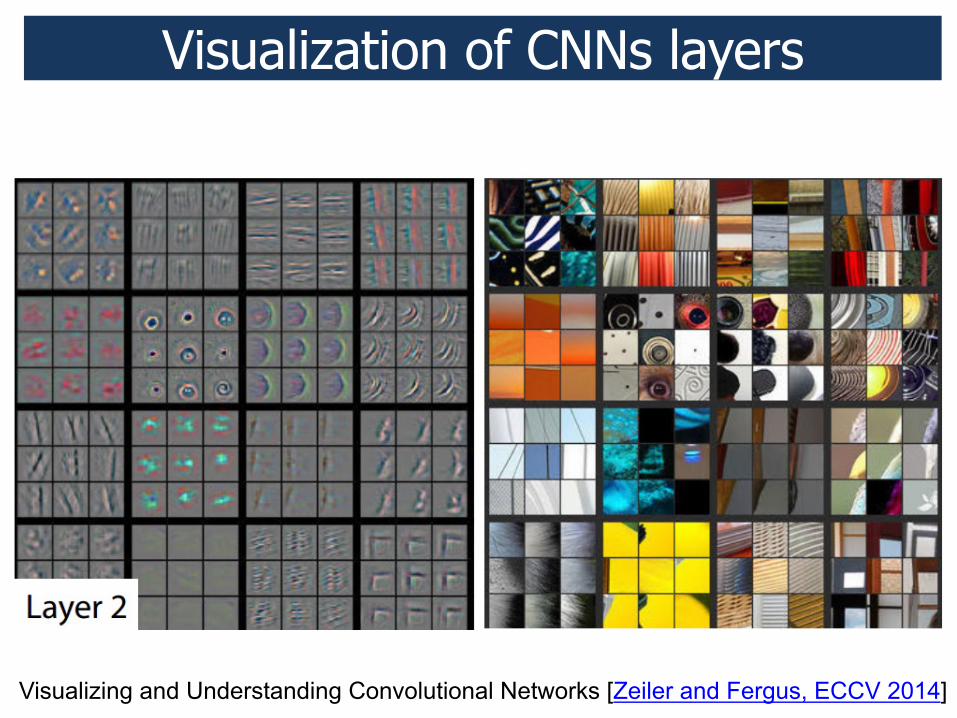
Layer 2
Visualizing and Understanding Convolutional Networks [Zeiler and Fergus, ECCV 2014]
Visualization of CNNs layers

Layer 3
Visualizing and Understanding Convolutional Networks [Zeiler and Fergus, ECCV 2014]
Visualization of CNNs layers
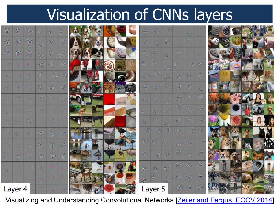
Layer 4 and 5
Visualizing and Understanding Convolutional Networks [Zeiler and Fergus, ECCV 2014]
Visualization of CNNs layers
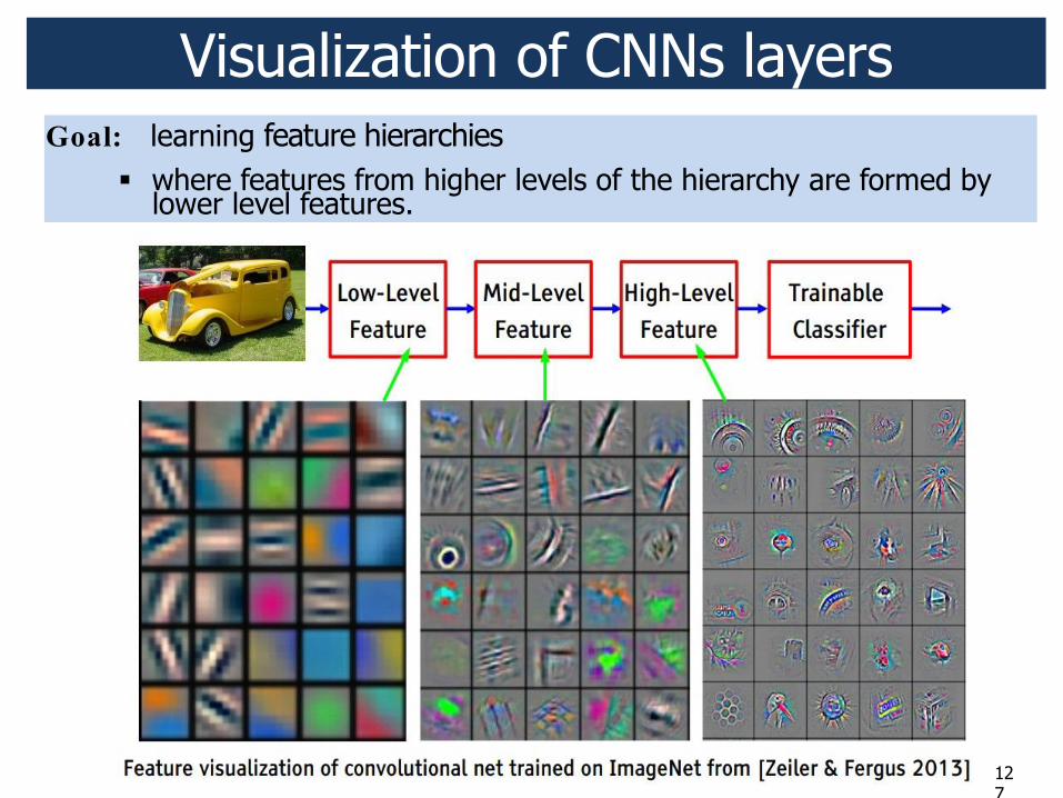
127
Visualization of CNNs layers Goal: learning feature hierarchies
" where features from higher levels of the hierarchy are formed by lower level features.
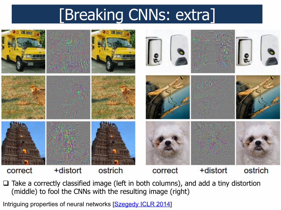
Breaking CNNs
Intriguing properties of neural networks [Szegedy ICLR 2014]
[Breaking CNNs: extra]
! Take a correctly classified image (left in both columns), and add a tiny distortion (middle) to fool the CNNs with the resulting image (right)
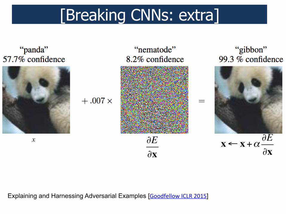
What is going on?
x x! x+! "E"x
!E!x
Explaining and Harnessing Adversarial Examples [D227>4::2E;FGHI;(C*J]
[Breaking CNNs: extra]
130
Credits
Many of the pictures, results, and other materials are taken from: Ruslan Salakhutdinov Joshua Bengio Geoffrey Hinton Yann LeCun Barnabás Póczos Aarti Singh Fei-Fei Li Andrej Karpathy Justin Johnson Rob Fergus Adriana Kovashka Leon Bottou

131
Thanks for your Attention! #$
132
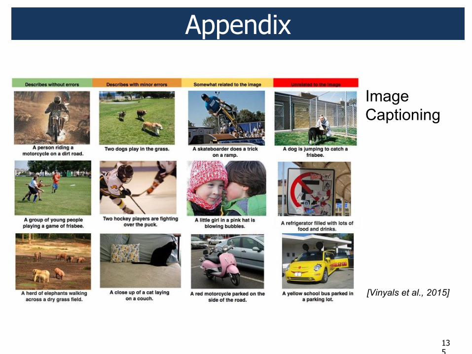
Appendix

133
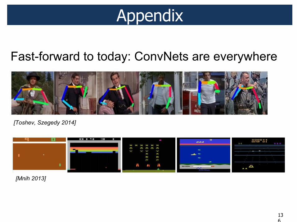
Appendix
134
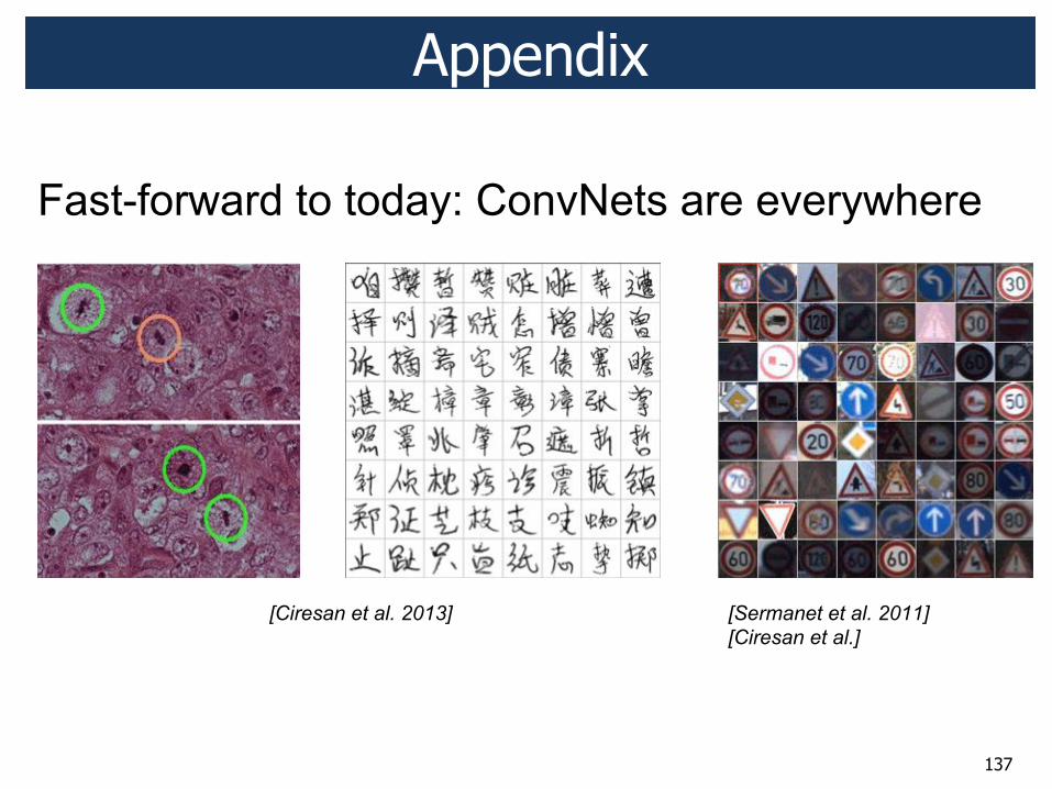
Appendix
135
Appendix
136
Appendix
137
Appendix
138
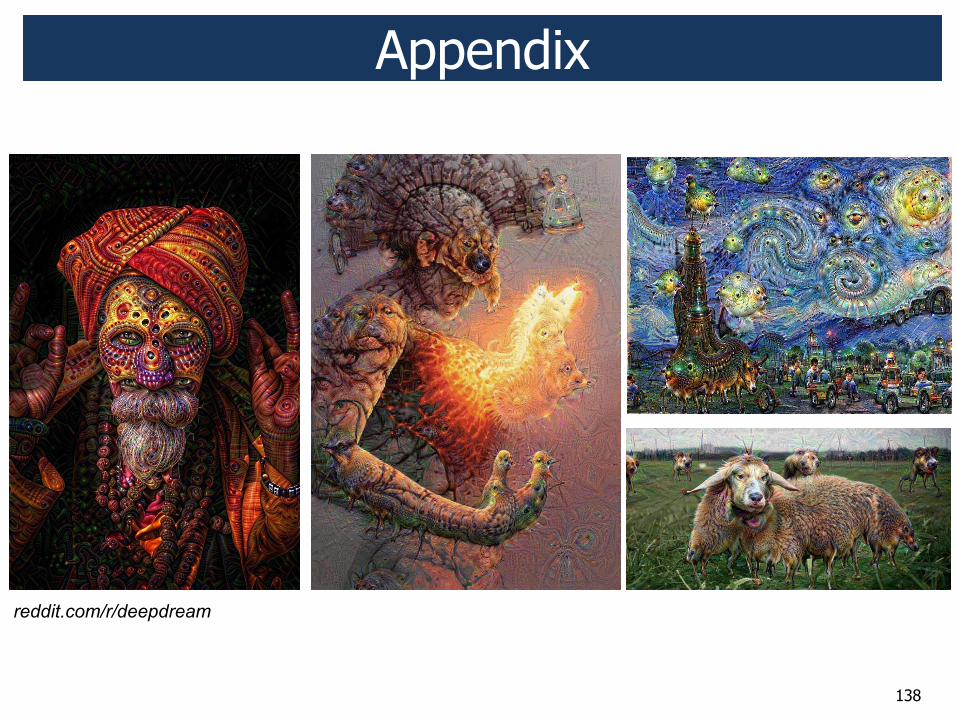
Appendix
139
Appendix ! I4'20?&4';
! K44#;H43?+.+-;&20?'4;3/;L/3+>2?7$;;!"#$%%&'()*+,'/3+>2?7,470%'A::310',!/8:;
! G20?'4;3/;M+.54?'./4;74;L!4?1?22@4$;!"#$%%.+>2,0'!4?1?22@4,&3%!:3?2&!4::4%+40?3:N+4/E2?@'%&2+/4+/,!/8:;
! K44#;H43?+.+-;'0884?;'&!22:;(C*J$;;!"#$%%5.742:4&/0?4',+4/%744#:43?+.+-(C*JN82+/?43:%;
! K44#;:43?+.+-;?4'20?&4'$;!"#$%%744#:43?+.+-,+4/%;
140
Appendix ! H.1?3?.4';
! G3O4;! &0736&2+5+4/(;! P2?&!;! P4+'2?Q:2E;
;;