Deep LearningLecture 4: Designing models to generalise

Chris G. WillcocksDurham University

Lecture Overview

1 Generalisation theoryuniversal approximation theoremempirical risk minimisationno free lunch theorem and Occam’s razorincreasing capacity through double descent

2 Function designnatural signalsconvolutional neural networksrecurrent neural networksdeep residual networks

3 Regularisationearly stopping and annealingthe effect on model capacitydata augmentationdropout and Tikhonov regularizationensembles

2 / 25

Generalisation theory universal approximation theorem

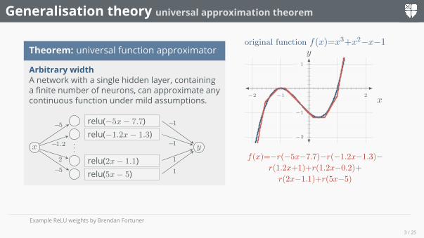
Theorem: universal function approximator

Arbitrary widthA network with a single hidden layer, containinga finite number of neurons, can approximate anycontinuous function under mild assumptions.

...

relu(−1.2x− 1.3)relu(−5x− 7.7)

relu(2x− 1.1)relu(5x− 5)

x y

−5

−1.2

2

−5

−1

−1

1

1

original function f(x)=x3+x2−x−1

−2 −1 1 2

−2

−1

1

x

y

f(x)=−r(−5x−7.7)−r(−1.2x−1.3)−r(1.2x+1)+r(1.2x−0.2)+

r(2x−1.1)+r(5x−5)

Example ReLU weights by Brendan Fortuner

3 / 25

Generalisation theory universal approximation theorem

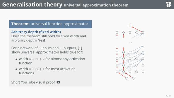
Theorem: universal function approximator

Arbitrary depth (fixed width)Does the theorem still hold for fixed width andarbitrary depth? Yes!

For a network of n inputs andm outputs, [1]show universal approximaton holds true for:

• width n+m+ 2 for almost any activationfunction

• width n+m+ 1 for most activationfunctions

Short YouTube visual proof v

· · ·

4 / 25

Generalisation theory empirical risk minimisation

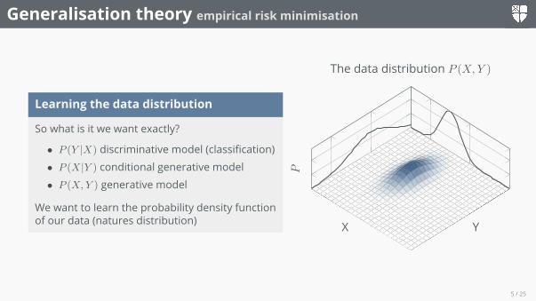
Learning the data distribution

So what is it we want exactly?

• P (Y |X) discriminative model (classification)• P (X|Y ) conditional generative model• P (X,Y ) generative model

We want to learn the probability density functionof our data (natures distribution) YX

P

The data distribution P (X,Y )

5 / 25

Generalisation theory empirical risk minimisation

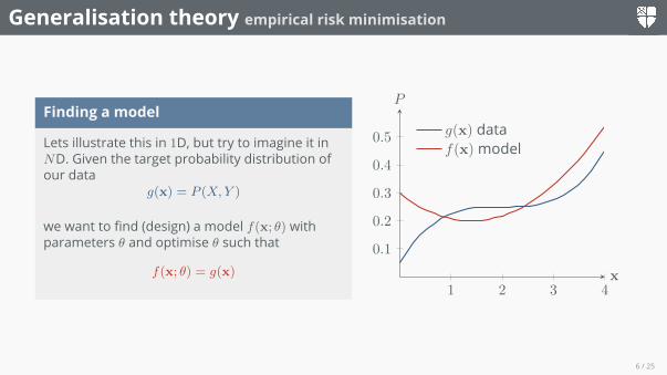
Finding a model

Lets illustrate this in 1D, but try to imagine it inND. Given the target probability distribution ofour data

g(x) = P (X,Y )

we want to find (design) a model f(x; θ) withparameters θ and optimise θ such that

f(x; θ) = g(x)

1 2 3 4

0.1

0.2

0.3

0.4

0.5

x

P

g(x) dataf(x)model

6 / 25

Generalisation theory empirical risk minimisation

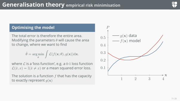
Optimising the model

The total error is therefore the entire area.Modifying the parameters θ will cause the areato change, where we want to find

θ̂ = argminθ

∫L(f(x; θ), g(x))dx.

where L is a ‘loss function’, e.g. a 0-1 loss functionL(x̂, x) = I(x̂ 6= x) or a mean squared error loss.

The solution is a function f that has the capacityto exactly represent g(x) 1 2 3 4

0.1

0.2

0.3

0.4

0.5

x

P

g(x) dataf(x)model

7 / 25

Generalisation theory empirical risk minimisation

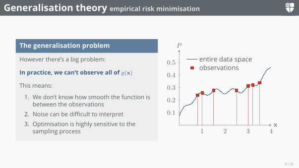
The generalisation problem

However there’s a big problem:

In practice, we can’t observe all of g(x)

This means:

1. We don’t know how smooth the function isbetween the observations

2. Noise can be difficult to interpret3. Optimisation is highly sensitive to the

sampling process 1 2 3 4

0.1

0.2

0.3

0.4

0.5

x

P

entire data spaceobservations

8 / 25

Generalisation theory empirical risk minimisation

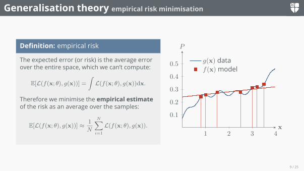
Definition: empirical risk

The expected error (or risk) is the average errorover the entire space, which we can’t compute:

E[L(f(x; θ), g(x))] =∫L(f(x; θ), g(x))dx.

Therefore we minimise the empirical estimateof the risk as an average over the samples:

E[L(f(x; θ), g(x))] ≈ 1

N

N∑i=1

L(f(x; θ), g(x)).1 2 3 4

0.1

0.2

0.3

0.4

0.5

x

P

g(x) dataf(x)model

9 / 25

Generalisation theory empirical risk minimisation

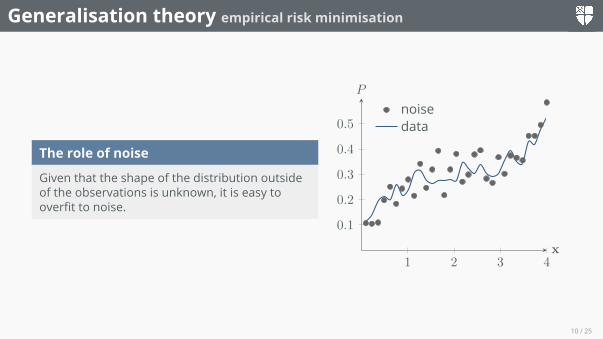
The role of noise

Given that the shape of the distribution outsideof the observations is unknown, it is easy tooverfit to noise.

1 2 3 4

0.1

0.2

0.3

0.4

0.5

x

P

noisedata

10 / 25

Generalisation theory empirical risk minimisation

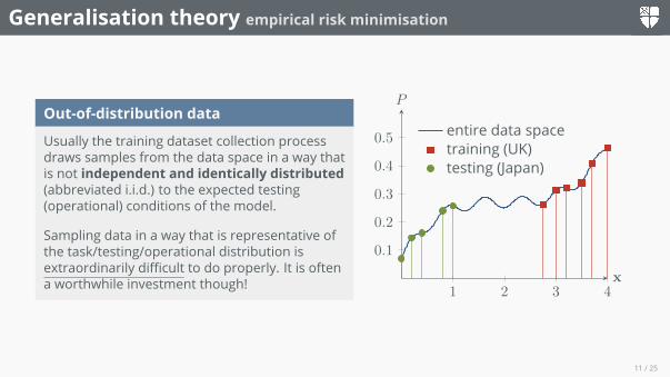
Out-of-distribution data

Usually the training dataset collection processdraws samples from the data space in a way thatis not independent and identically distributed(abbreviated i.i.d.) to the expected testing(operational) conditions of the model.

Sampling data in a way that is representative ofthe task/testing/operational distribution isextraordinarily difficult to do properly. It is oftena worthwhile investment though!

1 2 3 4

0.1

0.2

0.3

0.4

0.5

x

P

entire data spacetraining (UK)testing (Japan)

11 / 25

Generalisation theory no free lunch theorem and Occam’s razor

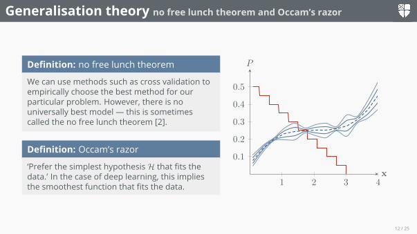
Definition: no free lunch theorem

We can use methods such as cross validation toempirically choose the best method for ourparticular problem. However, there is nouniversally best model — this is sometimescalled the no free lunch theorem [2].

Definition: Occam’s razor

‘Prefer the simplest hypothesisH that fits thedata.’ In the case of deep learning, this impliesthe smoothest function that fits the data. 1 2 3 4

0.1

0.2

0.3

0.4

0.5

x

P

12 / 25

Generalisation theory increasing capacity to double descent

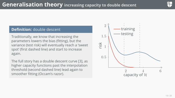
Definition: double descent

Traditionally, we know that increasing theparameters lowers the bias (fitting), but thevariance (test risk) will eventually reach a ‘sweetspot’ (first dashed line) and start to increaseagain.

The full story has a double descent curve [3], ashigher capacity functions past the interpolationthreshold (second dashed line) lead again tosmoother fitting (Occam’s razor).

2 4 6

0.5

1

1.5

2

capacity of H

risk

trainingtesting

13 / 25

Function design natural signals

Natural signals

In nature, the data signal follows patterns:

• There are repetitions in space and time• There are various symmetries• Signals are hierarchical

Therefore we can design our functions to fitthese patterns effectively

Further reading about deep learning through aphysics lens in [4]

14 / 25

Function design convolutional neural networks

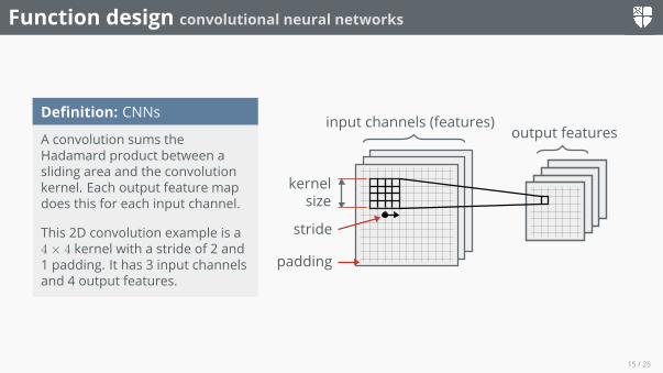
Definition: CNNs

A convolution sums theHadamard product between asliding area and the convolutionkernel. Each output feature mapdoes this for each input channel.

This 2D convolution example is a4× 4 kernel with a stride of 2 and1 padding. It has 3 input channelsand 4 output features.

kernelsize

stride

padding

input channels (features)output features

15 / 25

Function design convolutional neural networks

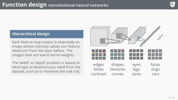
Hierarchical design

Each feature map output is essentially animage whose intensity values are ‘featuredetectors’ from the layer before. Theimages here are learnt kernel weights.

The ‘width’ vs ‘depth’ problem is based onwhat type of detectors you need from thedataset, such as to minimise the task risk.

edgesblobs

contrast

shapestexturescurves

eyeslegstyres

facesdogscars

16 / 25

Function design recurrent neural networks

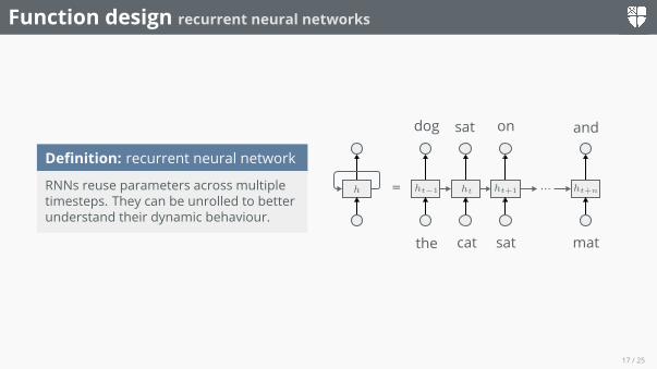
Definition: recurrent neural network

RNNs reuse parameters across multipletimesteps. They can be unrolled to betterunderstand their dynamic behaviour.

= ...h ht−1 ht ht+1 ht+n

the cat sat mat

dog sat on and

17 / 25

Function design deep residual networks

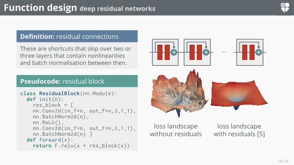
Definition: residual connections

These are shortcuts that skip over two orthree layers that contain nonlinearitiesand batch normalisation between then.

Pseudocode: residual blockclass ResidualBlock(nn.Module):

def init(n):res_block = [nn.Conv2d(in_f=n, out_f=n,3,1,1),nn.BatchNorm2d(n),nn.ReLU(),nn.Conv2d(in_f=n, out_f=n,3,1,1),nn.BatchNorm2d(n) ]

def forward(x):return F.relu(x + res_block(x))

+ + +...

loss landscapewithout residuals

loss landscapewith residuals [5]

18 / 25

Regularisation early stopping and annealing

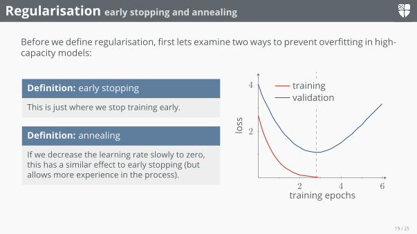
Before we define regularisation, first lets examine two ways to prevent overfitting in high-capacity models:

Definition: early stopping

This is just where we stop training early.

Definition: annealing

If we decrease the learning rate slowly to zero,this has a similar effect to early stopping (butallows more experience in the process).

2 4 6

2

4

training epochs

loss

trainingvalidation

19 / 25

Regularisation the effect on model capacity

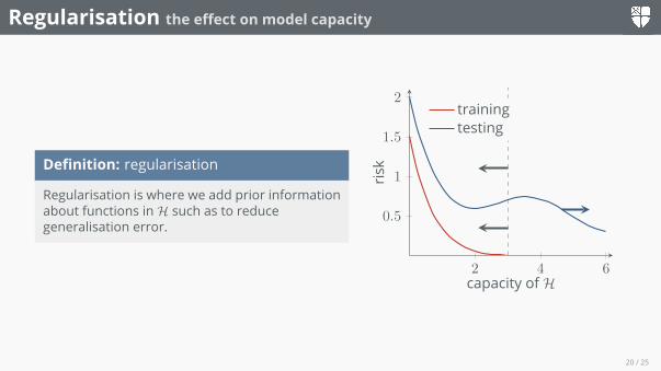
Definition: regularisation

Regularisation is where we add prior informationabout functions inH such as to reducegeneralisation error.

2 4 6

0.5

1

1.5

2

capacity of H

risk

trainingtesting

20 / 25

Regularisation data augmentation

Definition: data augmentation

If it is expected that small transformations (e.g.rotations, zooms, flips, blurs) will occur in testing,the training samples can be augmented.

However too much augmentation (e.g. too muchzoom) will result in poor fitting. In the extremecase it may even change the class label, forexample 180◦ rotations in MNIST:

21 / 25

Regularisation dropout and Tikhonov regularization

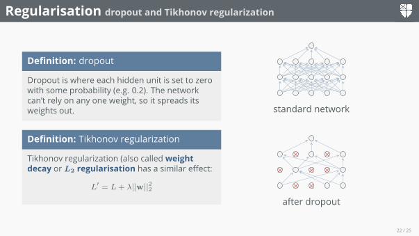
Definition: dropout

Dropout is where each hidden unit is set to zerowith some probability (e.g. 0.2). The networkcan’t rely on any one weight, so it spreads itsweights out.

Definition: Tikhonov regularization

Tikhonov regularization (also called weightdecay or L2 regularisation has a similar effect:

L′ = L+ λ||w||22

standard network

× ×× × ×× ×

after dropout

22 / 25

Regularisation ensembles

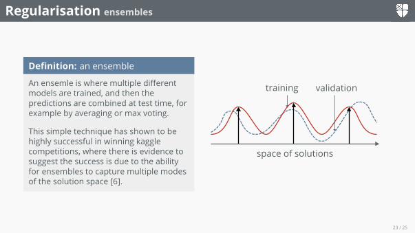
Definition: an ensemble

An ensemle is where multiple differentmodels are trained, and then thepredictions are combined at test time, forexample by averaging or max voting.

This simple technique has shown to behighly successful in winning kagglecompetitions, where there is evidence tosuggest the success is due to the abilityfor ensembles to capture multiple modesof the solution space [6].

space of solutions

training validation

23 / 25

Take Away Points

Summary

In summary, designing architectures:

• is a scientific process• choose the right functions to fit the data• choose your experiments carefully• consider the double descent graph• what do you know about the signal?• what does the task need?

24 / 25

References I

[1] Patrick Kidger and Terry Lyons. “Universal approximation with deep narrownetworks”. In: Conference on Learning Theory. 2020, pp. 2306–2327.

[2] Kevin P Murphy. Machine learning: a probabilistic perspective. MIT press, 2012.[3] Mikhail Belkin et al. “Reconciling modern machine-learning practice and the

classical bias–variance trade-off”. In:Proceedings of the National Academy of Sciences 116.32 (2019), pp. 15849–15854.

[4] Henry W Lin, Max Tegmark, and David Rolnick. “Why does deep and cheap learningwork so well?” In: Journal of Statistical Physics 168.6 (2017), pp. 1223–1247.

[5] Hao Li et al. “Visualizing the loss landscape of neural nets”. In:Advances in Neural Information Processing Systems. 2018, pp. 6389–6399.

[6] Stanislav Fort, Huiyi Hu, and Balaji Lakshminarayanan. “Deep ensembles: A losslandscape perspective”. In: arXiv preprint arXiv:1912.02757 (2019).

25 / 25