Deep Learning in Bioinformatics

Seonwoo Min1, Byunghan Lee1, and Sungroh Yoon1,2*

1Department of Electrical and Computer Engineering, Seoul National University, Seoul 08826, Korea 2Interdisciplinary Program in Bioinformatics, Seoul National University, Seoul 08826, Korea

Abstract

In the era of big data, transformation of biomedical big data into valuable knowledge has been

one of the most important challenges in bioinformatics. Deep learning has advanced rapidly

since the early 2000s and now demonstrates state-of-the-art performance in various fields.

Accordingly, application of deep learning in bioinformatics to gain insight from data has been

emphasized in both academia and industry. Here, we review deep learning in bioinformatics,

presenting examples of current research. To provide a useful and comprehensive perspective,

we categorize research both by the bioinformatics domain (i.e., omics, biomedical imaging,

biomedical signal processing) and deep learning architecture (i.e., deep neural networks,

convolutional neural networks, recurrent neural networks, emergent architectures) and present

brief descriptions of each study. Additionally, we discuss theoretical and practical issues of

deep learning in bioinformatics and suggest future research directions. We believe that this

review will provide valuable insights and serve as a starting point for researchers to apply deep

learning approaches in their bioinformatics studies.

*Corresponding author. Mailing address: 301-908, Department of Electrical and Computer Engineering, Seoul National University, Seoul 08826, Korea. E-mail: sryoon@snu.ac.kr. Phone: +82-2-880-1401.

Keywords

Deep learning, neural network, machine learning, bioinformatics, omics, biomedical imaging,

biomedical signal processing

Key Points

As a great deal of biomedical data have been accumulated, various machine algorithms

are now being widely applied in bioinformatics to extract knowledge from big data.

Deep learning, which has evolved from the acquisition of big data, the power of

parallel and distributed computing, and sophisticated training algorithms, has

facilitated major advances in numerous domains such as image recognition, speech

recognition, and natural language processing.

We review deep learning for bioinformatics and present research categorized by

bioinformatics domain (i.e., omics, biomedical imaging, biomedical signal processing)

and deep learning architecture (i.e., deep neural networks, convolutional neural

networks, recurrent neural networks, emergent architectures).

Furthermore, we discuss the theoretical and practical issues plaguing the applications

of deep learning in bioinformatics, including imbalanced data, interpretation,

hyperparameter optimization, multimodal deep learning, and training acceleration.

As a comprehensive review of existing works, we believe that this paper will provide

valuable insight and serve as a launching point for researchers to apply deep learning

approaches in their bioinformatics studies.

Author Description

Seonwoo Min is a M.S./Ph.D. candidate at Department of Electrical and Computer

Engineering, Seoul National University, Korea. His research areas include high-performance

bioinformatics, machine learning for biomedical big data, and deep learning.

Byunghan Lee is a Ph.D. candidate at Department of Electrical and Computer Engineering,

Seoul National University, Korea. His research areas include high-performance bioinformatics,

machine learning for biomedical big data, and data mining.

Sungroh Yoon is an associate professor at Department of Electrical and Computer Engineering,

Seoul National University, Seoul, Korea. He received his Ph.D. and postdoctoral training from

Stanford University, Stanford, USA. His research interests include machine learning and deep

learning for bioinformatics, and high-performance bioinformatics.

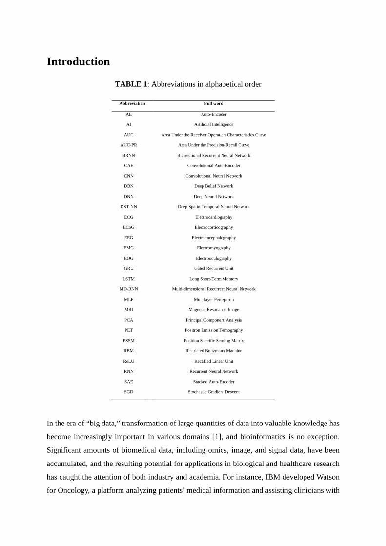
Introduction

TABLE 1: Abbreviations in alphabetical order

Abbreviation Full word

AE Auto-Encoder

AI Artificial Intelligence

AUC Area Under the Receiver Operation Characteristics Curve

AUC-PR Area Under the Precision-Recall Curve

BRNN Bidirectional Recurrent Neural Network

CAE Convolutional Auto-Encoder

CNN Convolutional Neural Network

DBN Deep Belief Network

DNN Deep Neural Network

DST-NN Deep Spatio-Temporal Neural Network

ECG Electrocardiography

ECoG Electrocorticography

EEG Electroencephalography

EMG Electromyography

EOG Electrooculography

GRU Gated Recurrent Unit

LSTM Long Short-Term Memory

MD-RNN Multi-dimensional Recurrent Neural Network

MLP Multilayer Perceptron

MRI Magnetic Resonance Image

PCA Principal Component Analysis

PET Positron Emission Tomography

PSSM Position Specific Scoring Matrix

RBM Restricted Boltzmann Machine

ReLU Rectified Linear Unit

RNN Recurrent Neural Network

SAE Stacked Auto-Encoder

SGD Stochastic Gradient Descent

In the era of “big data,” transformation of large quantities of data into valuable knowledge has

become increasingly important in various domains [1], and bioinformatics is no exception.

Significant amounts of biomedical data, including omics, image, and signal data, have been

accumulated, and the resulting potential for applications in biological and healthcare research

has caught the attention of both industry and academia. For instance, IBM developed Watson

for Oncology, a platform analyzing patients’ medical information and assisting clinicians with

treatment options [2, 3]. In addition, Google DeepMind, having achieved great success with

AlphaGo in the game of Go, recently launched DeepMind Health to develop effective

healthcare technologies [4, 5].

To extract knowledge from big data in bioinformatics, machine learning has been a widely used

and successful methodology. Machine learning algorithms use training data to uncover

underlying patterns, build models, and make predictions based on the best fit model. Indeed,

some well-known algorithms (i.e., support vector machines, random forests, hidden Markov

models, Bayesian networks, Gaussian networks) have been applied in genomics, proteomics,

systems biology, and numerous other domains [6].

[FIGURE 1]

The proper performance of conventional machine learning algorithms relies heavily on data

representations called features [7]. However, features are typically designed by human

engineers with extensive domain expertise, and identifying which features are more appropriate

for the given task remains difficult. Deep learning, a branch of machine learning, has recently

emerged based on big data, the power of parallel and distributed computing, and sophisticated

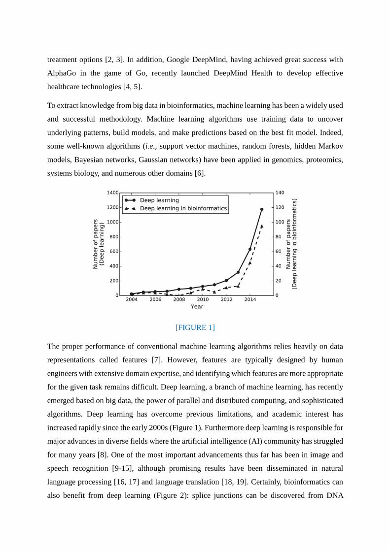
algorithms. Deep learning has overcome previous limitations, and academic interest has

increased rapidly since the early 2000s (Figure 1). Furthermore deep learning is responsible for

major advances in diverse fields where the artificial intelligence (AI) community has struggled

for many years [8]. One of the most important advancements thus far has been in image and

speech recognition [9-15], although promising results have been disseminated in natural

language processing [16, 17] and language translation [18, 19]. Certainly, bioinformatics can

also benefit from deep learning (Figure 2): splice junctions can be discovered from DNA

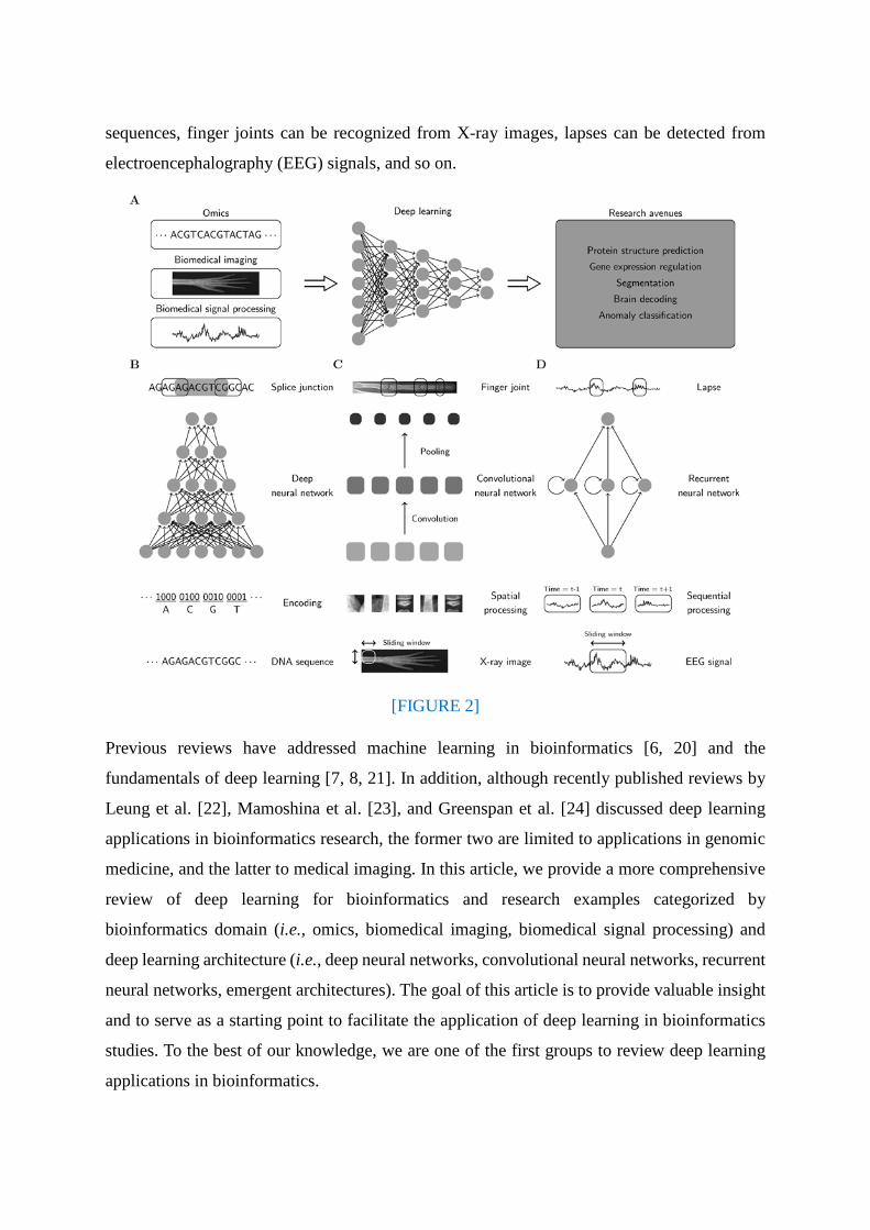
sequences, finger joints can be recognized from X-ray images, lapses can be detected from

electroencephalography (EEG) signals, and so on.

[FIGURE 2]

Previous reviews have addressed machine learning in bioinformatics [6, 20] and the

fundamentals of deep learning [7, 8, 21]. In addition, although recently published reviews by

Leung et al. [22], Mamoshina et al. [23], and Greenspan et al. [24] discussed deep learning

applications in bioinformatics research, the former two are limited to applications in genomic

medicine, and the latter to medical imaging. In this article, we provide a more comprehensive

review of deep learning for bioinformatics and research examples categorized by

bioinformatics domain (i.e., omics, biomedical imaging, biomedical signal processing) and

deep learning architecture (i.e., deep neural networks, convolutional neural networks, recurrent

neural networks, emergent architectures). The goal of this article is to provide valuable insight

and to serve as a starting point to facilitate the application of deep learning in bioinformatics

studies. To the best of our knowledge, we are one of the first groups to review deep learning

applications in bioinformatics.

Deep learning: a brief overview

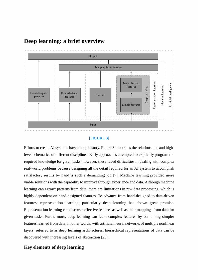
[FIGURE 3]

Efforts to create AI systems have a long history. Figure 3 illustrates the relationships and high-

level schematics of different disciplines. Early approaches attempted to explicitly program the

required knowledge for given tasks; however, these faced difficulties in dealing with complex

real-world problems because designing all the detail required for an AI system to accomplish

satisfactory results by hand is such a demanding job [7]. Machine learning provided more

viable solutions with the capability to improve through experience and data. Although machine

learning can extract patterns from data, there are limitations in raw data processing, which is

highly dependent on hand-designed features. To advance from hand-designed to data-driven

features, representation learning, particularly deep learning has shown great promise.

Representation learning can discover effective features as well as their mappings from data for

given tasks. Furthermore, deep learning can learn complex features by combining simpler

features learned from data. In other words, with artificial neural networks of multiple nonlinear

layers, referred to as deep learning architectures, hierarchical representations of data can be

discovered with increasing levels of abstraction [25].

Key elements of deep learning

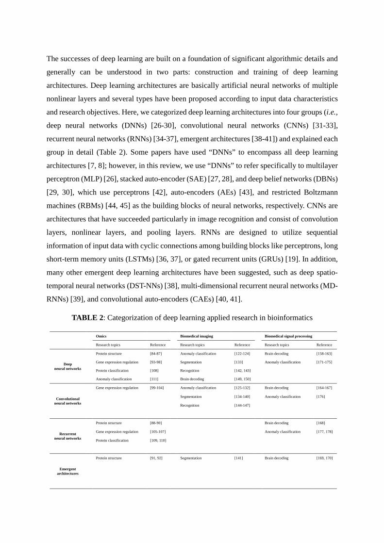
The successes of deep learning are built on a foundation of significant algorithmic details and

generally can be understood in two parts: construction and training of deep learning

architectures. Deep learning architectures are basically artificial neural networks of multiple

nonlinear layers and several types have been proposed according to input data characteristics

and research objectives. Here, we categorized deep learning architectures into four groups (i.e.,

deep neural networks (DNNs) [26-30], convolutional neural networks (CNNs) [31-33],

recurrent neural networks (RNNs) [34-37], emergent architectures [38-41]) and explained each

group in detail (Table 2). Some papers have used “DNNs” to encompass all deep learning

architectures [7, 8]; however, in this review, we use “DNNs” to refer specifically to multilayer

perceptron (MLP) [26], stacked auto-encoder (SAE) [27, 28], and deep belief networks (DBNs)

[29, 30], which use perceptrons [42], auto-encoders (AEs) [43], and restricted Boltzmann

machines (RBMs) [44, 45] as the building blocks of neural networks, respectively. CNNs are

architectures that have succeeded particularly in image recognition and consist of convolution

layers, nonlinear layers, and pooling layers. RNNs are designed to utilize sequential

information of input data with cyclic connections among building blocks like perceptrons, long

short-term memory units (LSTMs) [36, 37], or gated recurrent units (GRUs) [19]. In addition,

many other emergent deep learning architectures have been suggested, such as deep spatio-

temporal neural networks (DST-NNs) [38], multi-dimensional recurrent neural networks (MD-

RNNs) [39], and convolutional auto-encoders (CAEs) [40, 41].

TABLE 2: Categorization of deep learning applied research in bioinformatics

Omics Biomedical imaging Biomedical signal processing

Research topics Reference Research topics Reference Research topics Reference

Deep neural networks

Protein structure [84-87] Anomaly classification [122-124] Brain decoding [158-163]

Gene expression regulation [93-98] Segmentation [133] Anomaly classification [171-175]

Protein classification [108] Recognition [142, 143]

Anomaly classification [111] Brain decoding [149, 150]

Convolutional neural networks

Gene expression regulation [99-104] Anomaly classification [125-132] Brain decoding [164-167]

Segmentation [134-140] Anomaly classification [176]

Recognition [144-147]

Recurrent neural networks

Protein structure [88-90] Brain decoding [168]

Gene expression regulation [105-107] Anomaly classification [177, 178]

Protein classification [109, 110]

Emergent architectures

Protein structure [91, 92] Segmentation [141] Brain decoding [169, 170]

The goal of training deep learning architectures is optimization of the weight parameters in

each layer, which gradually combines simpler features into complex features so that the most

suitable hierarchical representations can be learned from data. A single cycle of the

optimization process is organized as follows [8]. First, given a training dataset, the forward

pass sequentially computes the output in each layer and propagates the function signals forward

through the network. In the final output layer, an objective loss function measures error

between the inferenced outputs and the given labels. To minimize the training error, the

backward pass uses the chain rule to backpropagate error signals and compute gradients with

respect to all weights throughout the neural network [46]. Finally, the weight parameters are

updated using optimization algorithms based on stochastic gradient descent (SGD) [47].

Whereas batch gradient descent performs parameter updates for each complete dataset, SGD

provides stochastic approximations by performing the updates for each small set of data

examples. Several optimization algorithms stem from SGD. For example, Adagrad [48] and

Adam [49] perform SGD while adaptively modifying learning rates based on update frequency

and moments of the gradients for each parameter, respectively.

Another core element in the training of deep learning architectures is regularization, which

refers to strategies intended to avoid overfitting and thus achieve good generalization

performance. For example, weight decay [50], a well-known conventional approach, adds a

penalty term to the objective loss function so that weight parameters converge to smaller

absolute values. Currently, the most widely used regularization approach is dropout [51].

Dropout randomly removes hidden units from neural networks during training and can be

considered an ensemble of possible subnetworks [52]. To enhance the capabilities of dropout,

a new activation function, maxout [53], and a variant of dropout for RNNs called rnnDrop [54],

have been proposed. Furthermore, recently proposed batch normalization [55] provides a new

regularization method through normalization of scalar features for each activation within a

mini-batch and learning each mean and variance as parameters.

Deep learning libraries

To actually implement deep learning algorithms, a great deal of attention to algorithmic

details is required. Fortunately, many open source deep learning libraries are available online

(Table 3). There are still no clear front-runners, and each library has its own strengths [56].

According to benchmark test results of CNNs, specifically AlexNet [33] implementation in

Baharampour et al. [57], Python-based Neon [58] shows a great advantage in the processing

speed. C++ based Caffe [59] and Lua-based Torch [60] offer great advantages in terms of

pre-trained models and functional extensionality, respectively. Python-based Theano [61, 62]

provides a low-level library to define and optimize mathematical expressions; moreover,

numerous higher-level wrappers such as Keras [63], Lasagne [64], and Blocks [65] have been

developed on top of Theano to provide more intuitive interfaces. Google recently released

the C++-based TensorFlow [66] with a Python interface. This library currently shows limited

performance but is undergoing continuous improvement, as heterogeneous distributed

computing is now supported. In addition, TensorFlow can also take advantage of Keras,

which provides an additional model-level interface.

TABLE 3: Comparison of deep learning libraries

Core Speed for batch* (ms) Multi-GPU Distributed Strengths [56, 57]

Caffe C++ 651.6 O X Pre-trained models supported

Neon Python 386.8 O X Speed

TensorFlow C++ 962.0 O O Heterogeneous distributed computing

Theano Python 733.5 X X Ease of use with higher-level wrappers

Torch Lua 506.6 O X Functional extensionality

Notes. Speed for batch* is based on the averaged processing times for AlexNet [33] with batch size of 256 on a single GPU [57]; Caffe, Neon, Theano, Torch was utilized with cuDNN v.3 while TensorFlow was utilized with cuDNN v.2

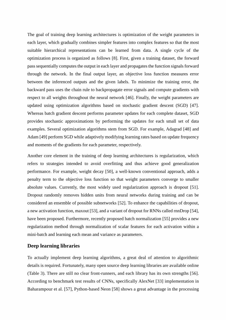
Deep neural networks

The basic structure of DNNs consists of an input layer, multiple hidden layers, and an output

layer (Figure 4). Once input data are given to the DNNs, output values are computed

sequentially along the layers of the network. At each layer, the input vector comprising the

output values of each unit in the layer below is multiplied by the weight vector for each unit in

the current layer to produce the weighted sum. Then, a nonlinear function, such as a sigmoid,

hyperbolic tangent, or rectified linear unit (ReLU) [67], is applied to the weighted sum to

compute the output values of the layer. The computation in each layer transforms the

representations in the layer below into slightly more abstract representations [8]. Based on the

types of layers used in DNNs and the corresponding learning method, DNNs can be classified

as MLP, SAE, or DBN.

[FIGURE 4]

MLP has a similar structure to the usual neural networks but includes more stacked layers. It is

trained in a purely supervised manner that uses only labeled data. Since the training method is

a process of optimization in high-dimensional parameter space, MLP is typically used when a

large number of labeled data are available [25].

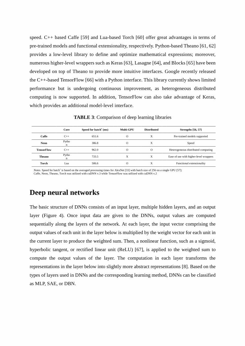
[FIGURE 5]

SAE and DBN use AEs and RBMs as building blocks of the architectures, respectively. The

main difference between these and MLP is that training is executed in two phases: unsupervised

pre-training and supervised fine-tuning. First, in unsupervised pre-training (Figure 5), the

layers are stacked sequentially and trained in a layer-wise manner as an AE or RBM using

unlabeled data. Afterwards, in supervised fine-tuning, an output classifier layer is stacked, and

the whole neural network is optimized by retraining with labeled data. Since both SAE and

DBN exploit unlabeled data and can help avoid overfitting, researchers are able to obtain fairly

regularized results, even when labeled data are insufficient as is common in the real world [68].

DNNs are renowned for their suitability in analyzing high-dimensional data. Given that

bioinformatics data are typically complex and high-dimensional, DNNs have great promise for

bioinformatics research. We believe DNNs, as hierarchical representation learning methods,

can discover previously unknown highly abstract patterns and correlations to provide insight

to better understand the nature of the data. However, it has occurred to us that the capabilities

of DNNs have not yet fully been exploited. Although the key characteristic of DNNs is that

hierarchical features are learned solely from data, human designed features have often been

given as inputs instead of raw data forms. We expect that the future progress of DNNs in

bioinformatics will come from investigations into proper ways to encode raw data and learn

suitable features from them.

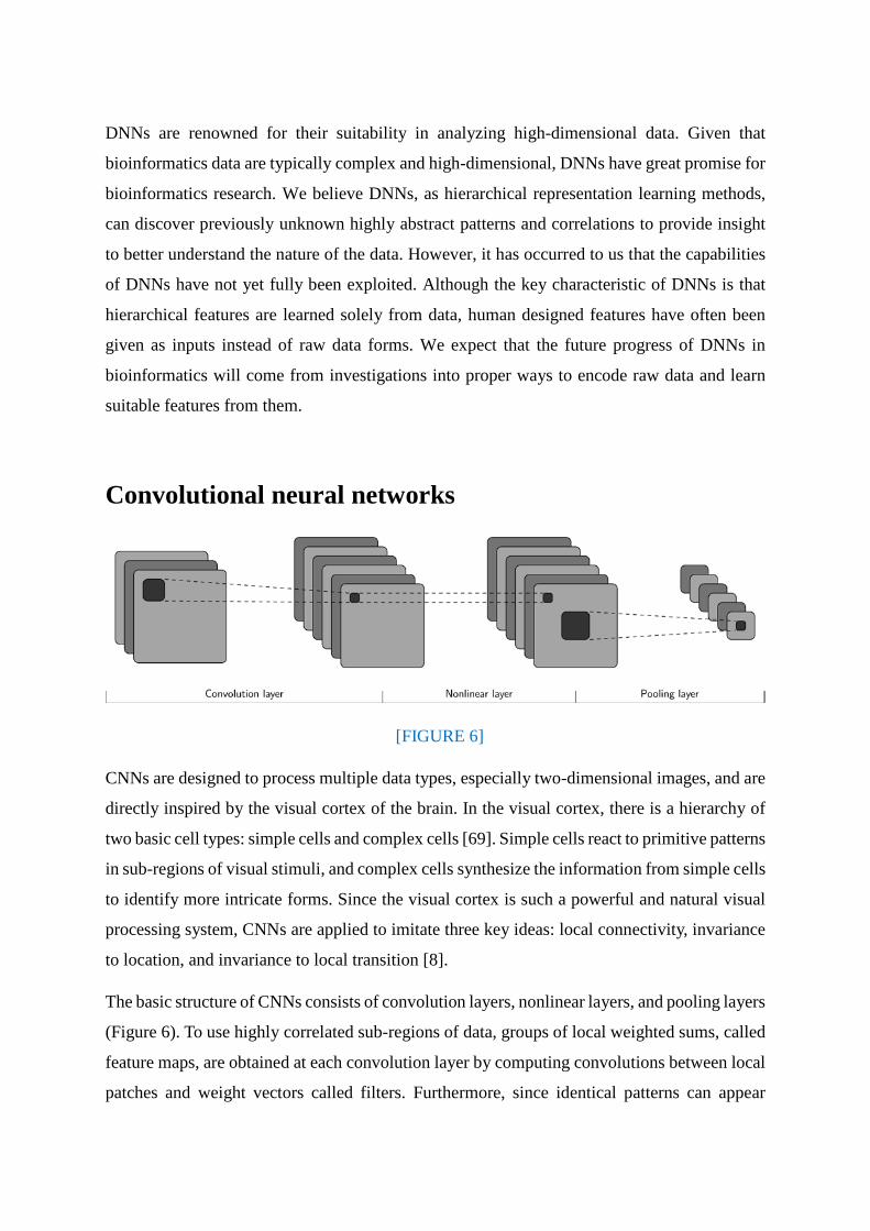
Convolutional neural networks

[FIGURE 6]

CNNs are designed to process multiple data types, especially two-dimensional images, and are

directly inspired by the visual cortex of the brain. In the visual cortex, there is a hierarchy of

two basic cell types: simple cells and complex cells [69]. Simple cells react to primitive patterns

in sub-regions of visual stimuli, and complex cells synthesize the information from simple cells

to identify more intricate forms. Since the visual cortex is such a powerful and natural visual

processing system, CNNs are applied to imitate three key ideas: local connectivity, invariance

to location, and invariance to local transition [8].

The basic structure of CNNs consists of convolution layers, nonlinear layers, and pooling layers

(Figure 6). To use highly correlated sub-regions of data, groups of local weighted sums, called

feature maps, are obtained at each convolution layer by computing convolutions between local

patches and weight vectors called filters. Furthermore, since identical patterns can appear

regardless of the location in the data, filters are applied repeatedly across the entire dataset,

which also improves training efficiency by reducing the number of parameters to learn. Then

nonlinear layers increase the nonlinear properties of feature maps. At each pooling layer,

maximum or average subsampling of non-overlapping regions in feature maps is performed.

This non-overlapping subsampling enables CNNs to handle somewhat different but

semantically similar features and thus aggregate local features to identify more complex

features.

Currently, CNNs are one of the most successful deep learning architectures owing to their

outstanding capacity to analyze spatial information. Thanks to their developments in the field

of object recognition, we believe the primary research achievements in bioinformatics will

come from the biomedical imaging domain. Despite the different data characteristics between

normal and biomedical imaging, CNN will nonetheless offer straightforward applications

compared to other domains. Indeed, CNNs also have great potential in omics and biomedical

signal processing. The three keys ideas of CNNs can be applied not only in a one-dimensional

grid to discover meaningful recurring patterns with small variance, such as genomic sequence

motifs, but also in two-dimensional grids, such as interactions within omics data and in time-

frequency matrices of biomedical signals. Thus, we believe the popularity and promise of

CNNs in bioinformatics applications will continue in the years ahead.

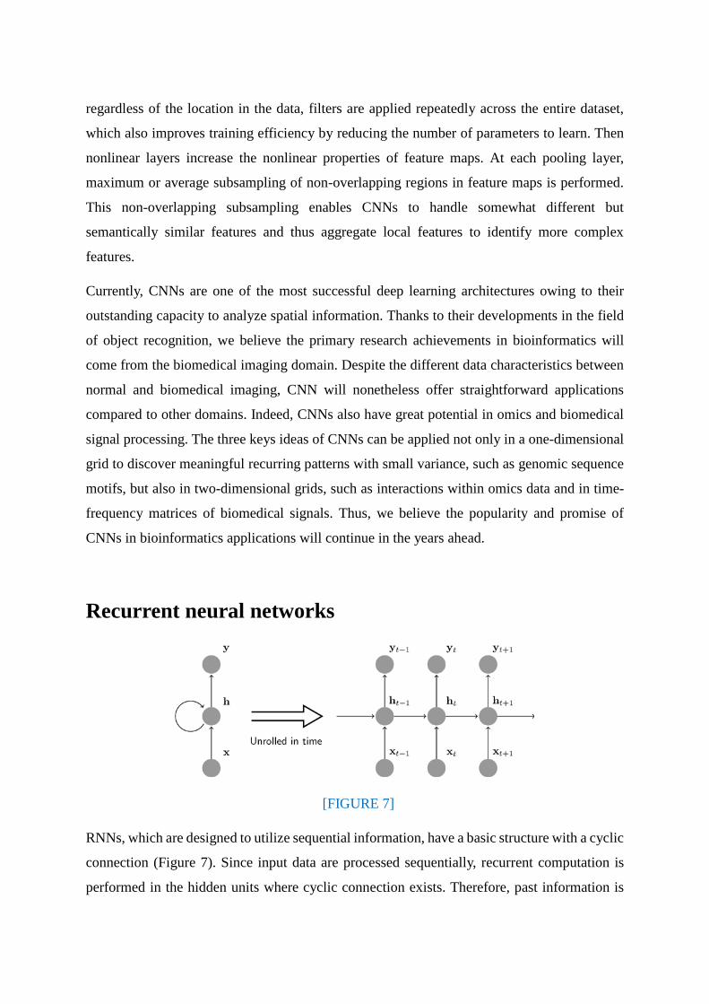
Recurrent neural networks

[FIGURE 7]

RNNs, which are designed to utilize sequential information, have a basic structure with a cyclic

connection (Figure 7). Since input data are processed sequentially, recurrent computation is

performed in the hidden units where cyclic connection exists. Therefore, past information is

implicitly stored in the hidden units called state vectors, and output for the current input is

computed considering all previous inputs using these state vectors [8]. Since there are many

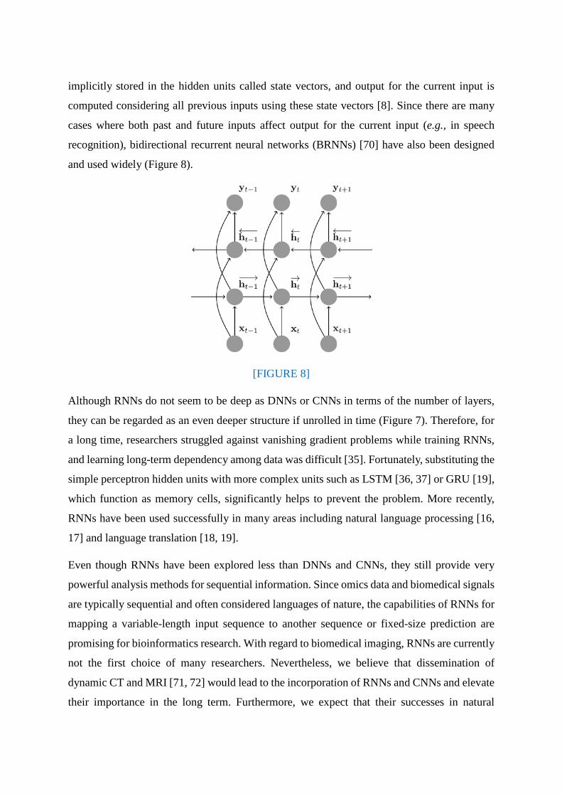
cases where both past and future inputs affect output for the current input (e.g., in speech

recognition), bidirectional recurrent neural networks (BRNNs) [70] have also been designed

and used widely (Figure 8).

[FIGURE 8]

Although RNNs do not seem to be deep as DNNs or CNNs in terms of the number of layers,

they can be regarded as an even deeper structure if unrolled in time (Figure 7). Therefore, for

a long time, researchers struggled against vanishing gradient problems while training RNNs,

and learning long-term dependency among data was difficult [35]. Fortunately, substituting the

simple perceptron hidden units with more complex units such as LSTM [36, 37] or GRU [19],

which function as memory cells, significantly helps to prevent the problem. More recently,

RNNs have been used successfully in many areas including natural language processing [16,

17] and language translation [18, 19].

Even though RNNs have been explored less than DNNs and CNNs, they still provide very

powerful analysis methods for sequential information. Since omics data and biomedical signals

are typically sequential and often considered languages of nature, the capabilities of RNNs for

mapping a variable-length input sequence to another sequence or fixed-size prediction are

promising for bioinformatics research. With regard to biomedical imaging, RNNs are currently

not the first choice of many researchers. Nevertheless, we believe that dissemination of

dynamic CT and MRI [71, 72] would lead to the incorporation of RNNs and CNNs and elevate

their importance in the long term. Furthermore, we expect that their successes in natural

language processing will lead RNNs to be applied in biomedical text analysis [73] and that

employing an attention mechanism [74-77] will improve performance and extract more

relevant information from bioinformatics data.

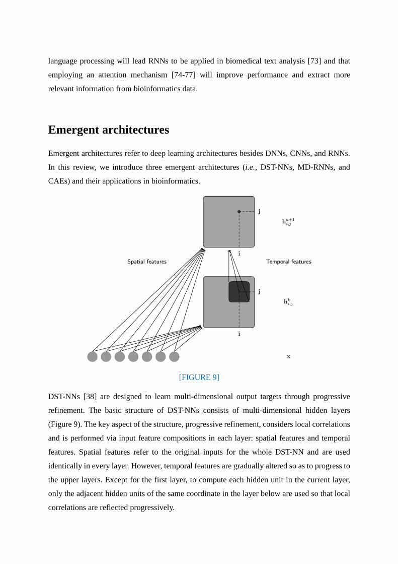
Emergent architectures

Emergent architectures refer to deep learning architectures besides DNNs, CNNs, and RNNs.

In this review, we introduce three emergent architectures (i.e., DST-NNs, MD-RNNs, and

CAEs) and their applications in bioinformatics.

[FIGURE 9]

DST-NNs [38] are designed to learn multi-dimensional output targets through progressive

refinement. The basic structure of DST-NNs consists of multi-dimensional hidden layers

(Figure 9). The key aspect of the structure, progressive refinement, considers local correlations

and is performed via input feature compositions in each layer: spatial features and temporal

features. Spatial features refer to the original inputs for the whole DST-NN and are used

identically in every layer. However, temporal features are gradually altered so as to progress to

the upper layers. Except for the first layer, to compute each hidden unit in the current layer,

only the adjacent hidden units of the same coordinate in the layer below are used so that local

correlations are reflected progressively.

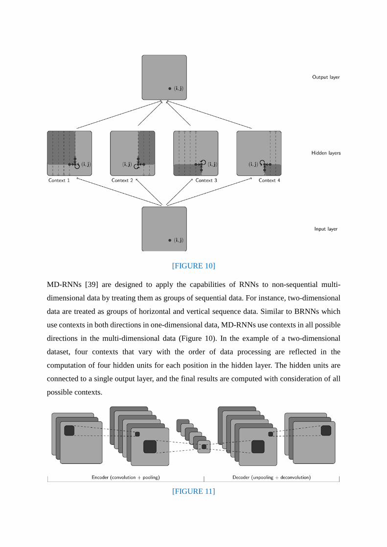
[FIGURE 10]

MD-RNNs [39] are designed to apply the capabilities of RNNs to non-sequential multi-

dimensional data by treating them as groups of sequential data. For instance, two-dimensional

data are treated as groups of horizontal and vertical sequence data. Similar to BRNNs which

use contexts in both directions in one-dimensional data, MD-RNNs use contexts in all possible

directions in the multi-dimensional data (Figure 10). In the example of a two-dimensional

dataset, four contexts that vary with the order of data processing are reflected in the

computation of four hidden units for each position in the hidden layer. The hidden units are

connected to a single output layer, and the final results are computed with consideration of all

possible contexts.

[FIGURE 11]

CAEs [40, 41] are designed to utilize the advantages of both AE and CNNs so that it can learn

good hierarchical representations of data reflecting spatial information and be well regularized

by unsupervised training (Figure 11). In training of AEs, reconstruction error is minimized

using an encoder and decoder, which extract feature vectors from input data and recreate the

data from the feature vectors, respectively. In CNNs, convolution and pooling layers can be

regarded as a type of encoder. Therefore, the CNN encoder and decoder consisting of

deconvolution and unpooling layers are integrated to form a CAE and are trained in the same

manner as in AE.

Deep learning is a rapidly growing research area, and a plethora of new deep learning

architecture is being proposed but awaits wide applications in bioinformatics. Newly proposed

architectures have different advantages from existing architectures, so we expect them to

produce promising results in various research areas. For example, the progressive refinement

of DST-NNs fits the dynamic folding process of proteins and can be effectively utilized in

protein structure prediction [38]; the capabilities of MD-RNNs are suitable for segmentation

of biomedical images since segmentation requires interpretation of local and global contexts;

the unsupervised representation learning with consideration of spatial information in CAEs can

provide great advantages in discovering recurring patterns in limited and imbalanced

bioinformatics data.

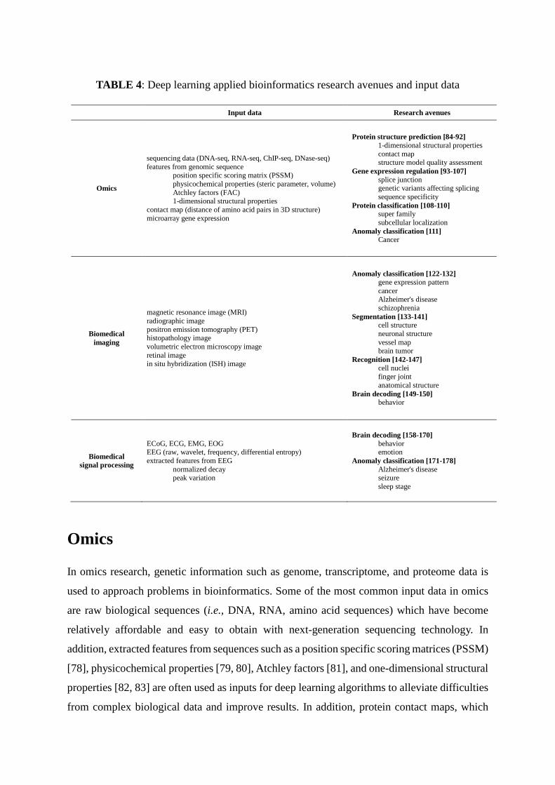
TABLE 4: Deep learning applied bioinformatics research avenues and input data

Input data Research avenues

Omics

sequencing data (DNA-seq, RNA-seq, ChIP-seq, DNase-seq) features from genomic sequence position specific scoring matrix (PSSM) physicochemical properties (steric parameter, volume) Atchley factors (FAC) 1-dimensional structural properties contact map (distance of amino acid pairs in 3D structure) microarray gene expression

Protein structure prediction [84-92] 1-dimensional structural properties contact map structure model quality assessment Gene expression regulation [93-107] splice junction genetic variants affecting splicing sequence specificity Protein classification [108-110] super family subcellular localization Anomaly classification [111] Cancer

Biomedical imaging

magnetic resonance image (MRI) radiographic image positron emission tomography (PET) histopathology image volumetric electron microscopy image retinal image in situ hybridization (ISH) image

Anomaly classification [122-132] gene expression pattern cancer Alzheimer's disease schizophrenia Segmentation [133-141] cell structure neuronal structure vessel map brain tumor Recognition [142-147] cell nuclei finger joint anatomical structure Brain decoding [149-150] behavior

Biomedical signal processing

ECoG, ECG, EMG, EOG EEG (raw, wavelet, frequency, differential entropy) extracted features from EEG normalized decay peak variation

Brain decoding [158-170] behavior emotion Anomaly classification [171-178] Alzheimer's disease seizure sleep stage

Omics

In omics research, genetic information such as genome, transcriptome, and proteome data is

used to approach problems in bioinformatics. Some of the most common input data in omics

are raw biological sequences (i.e., DNA, RNA, amino acid sequences) which have become

relatively affordable and easy to obtain with next-generation sequencing technology. In

addition, extracted features from sequences such as a position specific scoring matrices (PSSM)

[78], physicochemical properties [79, 80], Atchley factors [81], and one-dimensional structural

properties [82, 83] are often used as inputs for deep learning algorithms to alleviate difficulties

from complex biological data and improve results. In addition, protein contact maps, which

present distances of amino acid pairs in their three-dimensional structure, and microarray gene

expression data are also used according to the characteristics of interest. We categorized the

topics of interest in omics into four groups (Table 4). One of the most researched problems is

protein structure prediction, which aims to predict the secondary structure or contact map of a

protein [84-92]. Gene expression regulation [93-107], including splice junctions or RNA

binding proteins, and protein classification [108-110], including super family or subcellular

localization, are also actively investigated. Furthermore, anomaly classification [111]

approaches have been used with omics data to detect cancer.

Deep neural networks

DNNs have been widely applied in protein structure prediction [84-87] research. Since

complete prediction in three-dimensional space is complex and challenging, several studies

have used simpler approaches, such as predicting the secondary structure or torsion angles of

protein. For instance, Heffernan et al. [85] applied SAE to protein amino acid sequences to

solve prediction problems for secondary structure, torsion angle, and accessible surface area.

In another study, Spencer et al. [86] applied DBN to amino acid sequences along with PSSM

and Atchley factors to predict protein secondary structure. DNNs have also shown great

capabilities in the area of gene expression regulation [93-98]. For example, Lee et al. [94]

utilized DBN in splice junction prediction, a major research avenue in understanding gene

expression [112], and proposed a new DBN training method called boosted contrastive

divergence for imbalanced data and a new regularization term for sparsity of DNA sequences;

their work showed not only significantly improved performance but also the ability to detect

subtle non-canonical splicing signals. Moreover, Chen et al. [96] applied MLP to both

microarray and RNA-seq expression data to infer expression of up to 21000 target genes from

only 1000 landmark genes. In terms of protein classification, Asgari et al. [108] adopted the

skip-gram model, a widely known method in natural language processing, that can be

considered a variant of MLP, and showed that it could effectively learn a distributed

representation of biological sequences with general use for many omics applications, including

protein family classification. For anomaly classification, Fakoor et al. [111] used principal

component analysis (PCA) [113] to reduce the dimensionality of microarray gene expression

data and applied SAE to classify various cancers, including acute myeloid leukemia, breast

cancer, and ovarian cancer.

Convolutional neural networks

Relatively few studies have used CNNs to solve problems involving biological sequences,

specifically gene expression regulation problems [99-104]; nevertheless, those have introduced

the strong advantages of CNNs, showing their great promise for future research. First, an initial

convolution layer can powerfully capture local sequence patterns and can be considered a motif

detector for which PSSMs are solely learned from data instead of hard-coded. The depth of

CNNs enables learning more complex patterns and can capture longer motifs, integrate

cumulative effects of observed motifs, and eventually learn sophisticated regulatory codes

[114]. Moreover, CNNs are suited to exploit the benefits of multitask joint learning. By training

CNNs to simultaneously predict closely related factors, features with predictive strengths are

more efficiently learned and shared across different tasks.

For example, as an early approach, Denas et al. [99] preprocessed ChIP-seq data into a two-

dimensional matrix with the rows as transcription factor activity profiles for each gene and

exploited a two-dimensional CNN similar to its use in image processing. Recently, more studies

focused on directly using one-dimensional CNNs with biological sequence data. Alipanahi et

al. [100] and Kelley et al. [103] proposed CNN-based approaches for transcription factor

binding site prediction and 164 cell-specific DNA accessibility multitask prediction,

respectively; both groups presented downstream applications for disease-associated genetic

variant identification. Furthermore, Zeng et al. [102] performed a systematic exploration of

CNN architectures for transcription factor binding site prediction and showed that the number

of convolutional filters is more important than the number of layers for motif-based tasks. Zhou

et al. [104] developed a CNN-based algorithmic framework, DeepSEA, that performs multitask

joint learning of chromatin factors (i.e., transcription factor binding, DNase I sensitivity,

histone-mark profile) and prioritizes expression quantitative trait loci and disease-associated

genetic variants based on the predictions.

Recurrent neural networks

RNNs are expected to be an appropriate deep learning architecture because biological

sequences have variable lengths, and their sequential information has great importance. Several

studies have applied RNNs to protein structure prediction [88-90], gene expression regulation

[105-107], and protein classification [109, 110]. In early studies, Baldi et al. [88] used BRNNs

with perceptron hidden units in protein secondary structure prediction. Thereafter, the

improved performance of LSTM hidden units became widely recognized, so Sønderby et al.

[110] applied BRNNs with LSTM hidden units and a one-dimensional convolution layer to

learn representations from amino acid sequences and classify the subcellular locations of

proteins. Furthermore, Park et al. [105] and Lee et al. [107] exploited RNNs with LSTM hidden

units in microRNA identification and target prediction and obtained significantly improved

accuracy relative to state-of-the-art approaches demonstrating the high capacity of RNNs to

analyze biological sequences.

Emergent architectures

Emergent architectures have been used in protein structure prediction research [91, 92],

specifically in contact map prediction. Di Lena et al. [91] applied DST-NNs using spatial

features including protein secondary structure, orientation probability, and alignment

probability. Additionally, Baldi et al. [92] applied MD-RNNs to amino acid sequences,

correlated profiles, and protein secondary structures.

Biomedical imaging

Biomedical imaging [115] is another an actively researched domain with wide application of

deep learning in general image-related tasks. Most biomedical images used for clinical

treatment of patients—magnetic resonance imaging (MRI) [116, 117], radiographic imaging

[118, 119], positron emission tomography (PET) [120], and histopathology imaging [121]—

have been used as input data for deep learning algorithms. We categorized the research avenues

in biomedical imaging into four groups (Table 4). One of the most researched problems is

anomaly classification [122-132] to diagnose diseases such as cancer or schizophrenia. As in

general image-related tasks, segmentation [133-141] (i.e., partitioning specific structures such

as cellular structures or a brain tumor) and recognition [142-147] (i.e., detection of cell nuclei

or a finger joint) are studied frequently in biomedical imaging. Studies of popular high content

screening [148], which involves quantifying microscopic images for cell biology, are covered

in the former groups [128, 134, 137]. Additionally, cranial MRIs have been used in brain

decoding [149, 150] to interpret human behavior or emotion.

Deep neural networks

In terms of biomedical imaging, DNNs have been applied in several research areas, including

anomaly classification [122-124], segmentation [133], recognition [142, 143], and brain

decoding [149, 150]. Plis et al. [122] classified schizophrenia patients from brain MRIs using

DBN, and Xu et al. [142] used SAE to detect cell nuclei from histopathology images.

Interestingly, similar to handwritten digit image recognition, Van Gerven et al. [149] classified

handwritten digit images with DBN not by analyzing the images themselves but by indirectly

analyzing indirectly functional MRIs of participants who are looking at the digit images.

Convolutional neural networks

The largest number of studies have been conducted in biomedical imaging, since these avenues

are similar to general image-related tasks. In anomaly classification [125-132], Roth et al. [125]

applied CNNs to three different CT image datasets to classify sclerotic metastases, lymph nodes,

and colonic polyps. Additionally, Ciresan et al. [128] used CNNs to detect mitosis in breast

cancer histopathology images, a crucial approach for cancer diagnosis and assessment. PET

images of esophageal cancer were used by Ypsilantis et al. [129] to predict responses to

neoadjuvant chemotherapy. Other applications of CNNs can be found in segmentation [134-

140] and recognition [144-147]. For example, Ning et al. [134] studied pixel-wise segmentation

patterns of the cell wall, cytoplasm, nuclear membrane, nucleus, and outside media using

microscopic image, and Havaei et al. [139] proposed a cascaded CNN architecture exploiting

both local and global contextual features and performed brain tumor segmentation from MRIs.

For recognition, Cho et al. [144] researched anatomical structure recognition among CT images,

and Lee et al. [145] proposed a CNN-based finger joint detection system, FingerNet, which is

a crucial step for medical examinations of bone age, growth disorders, and rheumatoid arthritis

[151].

Recurrent neural networks

Traditionally, images are considered data that involve internal correlations or spatial

information rather than sequential information. Treating biomedical images as non-sequential

data, most studies in biomedical imaging have chosen approaches involving DNNs or CNNs

instead of RNNs.

Emergent architectures

Attempts to apply the unique capabilities of RNNs to image data using augmented RNN

structures have continued. MD-RNNs [39] have been applied beyond two-dimensional images

to three-dimensional images. For example, Stollenga et al. [141] applied MD-RNNs to three-

dimensional electron microscopy images and MRIs to segment neuronal structures.

Biomedical signal processing

Biomedical signal processing [115] is a domain where researchers use recorded electrical

activity from the human body to solve problems in bioinformatics. Various data from EEG

[152], electrocorticography (ECoG) [153], electrocardiography (ECG) [154],

electromyography (EMG) [155], and electrooculography (EOG) [156, 157] have been used,

with most studies focusing on EEG activity so far. Because recorded signals are usually noisy

and include many artifacts, raw signals are often decomposed into wavelet or frequency

components before they are used as input in deep learning algorithms. In addition, human-

designed features like normalized decay and peak variation are used in some studies to improve

the results. We categorized the research avenues in biomedical signal processing into two

groups (Table 4): brain decoding [158-170] using EEG signals and anomaly classification [171-

178] to diagnose diseases.

Deep neural networks

Since biomedical signals usually contain noise and artifacts, decomposed features are more

frequently used than raw signals. In brain decoding [158-163], An et al. [159] applied DBN to

the frequency components of EEG signals to classify left- and right-hand motor imagery skills.

Moreover, Jia et al. [161] and Jirayucharoensak et al. [163] used DBN and SAE, respectively,

for emotion classification. In anomaly classification [171-175], Huanhuan et al. [171]

published one of the few studies applying DBN to ECG signals and classified each beat into

either a normal or abnormal beat. A few studies have used raw EEG signals. Wulsin et al. [172]

analyzed individual second-long waveform abnormalities using DBN with both raw EEG

signals and extracted features as inputs, whereas Zhao et al. [174] used only raw EEG signals

as inputs for DBN to diagnose Alzheimer’s disease.

Convolutional neural networks

Raw EEG signals have been analyzed in brain decoding [164-167] and anomaly classification

[176] via CNNs, which perform one-dimensional convolutions. For instance, Stober et al. [165]

classified the rhythm type and genre of music that participants listened to, and Cecotti et al.

[167] classified characters that the participants viewed. Another approach to apply CNNs to

biomedical signal processing was reported by Mirowski et al. [176], who extracted features

such as phase-locking synchrony and wavelet coherence and coded them as pixel colors to

formulate two-dimensional patterns. Then, ordinary two-dimensional CNNs, like the one used

in biomedical imaging, were used to predict seizures.

Recurrent neural networks

Since biomedical signals represent naturally sequential data, RNNs are an appropriate deep

learning architecture to analyze data and are expected to produce promising results. To present

some of the studies in brain decoding [168] and anomaly classification [177, 178], Petrosian et

al. [177] applied perceptron RNNs to raw EEG signals and corresponding wavelet decomposed

features to predict seizures. In addition, Davidson et al. [178] used LSTM RNNs on EEG log-

power spectra features to detect lapses.

Emergent architectures

CAE has been applied in a few brain decoding studies [169, 170]. Wang et al. [169] performed

finger flex and extend classifications using raw ECoG signals. In addition, Stober et al. [170]

classified musical rhythms that participants listened to with raw EEG signals.

Discussion

Limited and imbalanced data

Considering the necessity of optimizing a tremendous number of weight parameters in neural

networks, most deep learning algorithms have assumed sufficient and balanced data.

Unfortunately, however, this is usually not true for problems in bioinformatics. Complex and

expensive data acquisition processes limit the size of bioinformatics datasets. In addition, such

processes often show significantly unequal class distributions, where an instance from one class

is significantly higher than instances from other classes [179]. For example in clinical or

disease-related cases, there is inevitably less data from treatment groups than from the normal

(control) group. The former are also rarely disclosed to the public due to privacy restrictions

and ethical requirements creating a further imbalance in available data [180].

A few assessment metrics have been used to clearly observe how limited and imbalanced data

might compromise the performance of deep learning [181]. While accuracy often gives

misleading results, the F-measure, the harmonic mean of precision and recall, provides more

insightful performance scores. To measure performance over different class distributions, the

area under the receiver operating characteristic curve (AUC) and the area under the precision-

recall curve (AUC-PR) are commonly used. These two measures are strongly correlated such

that a curve dominates in one measure if and only if it dominates in the other. Nevertheless, in

contrast with AUC-PR, AUC might present a more optimistic view of performance, since false

positive rates in the receiver operating characteristic curve fail to capture large changes of false

positives if classes are negatively skewed [182].

Solutions to limited and imbalanced data can be divided into three major groups [181, 183] :

data preprocessing, cost-sensitive learning and algorithmic modification. Data preprocessing

typically provides a better dataset through sampling or basic feature extraction. Sampling

methods balance the distribution of imbalanced data, and several approaches have been

proposed, including informed undersampling [184], the synthetic minority oversampling

technique [185], and cluster-based sampling [186]. For example, Li et al. [127] and Roth et al.

[146] performed enrichment analyses of CT images through spatial deformations such as

random shifting and rotation. Although basic feature extraction methods deviate from the

concept of deep learning, they are occasionally used to lessen the difficulties of learning from

limited and imbalanced data. Research in bioinformatics using human designed features as

input data such as PSSM from genomics sequences or wavelet energy from EEG signals can

be understood in the same context [86, 92, 172, 176].

Cost-sensitive learning methods define different costs for misclassifying data examples from

individual classes to solve the limited and imbalanced data problems. Cost sensitivity can be

applied in an objective loss function of neural networks either explicitly or implicitly [187].

For example, we can explicitly replace the objective loss function to reflect class imbalance or

implicitly modify the learning rates according to data instance classes during training.

Algorithmic modification methods accommodate learning algorithms to increase their

suitability for limited and imbalanced data. A simple and effective approach is adoption of pre-

training. Unsupervised pre-training can be a great help to learn representation for each class

and to produce more regularized results [68]. In addition, transfer learning, which consists of

pre-training with sufficient data from similar but different domains and fine-tuning with real

data, has great advantages [24, 188]. For instance, Lee et al. [107] proposed a microRNA target

prediction method, which exploits unsupervised pre-training with RNN based AE, and

achieved a >25% increase in F-measure compared to the existing alternatives. Bar et al. [132]

performed transfer learning using natural images from the ImageNet database [189] as pre-

training data and fine-tuned with chest X-ray images to identify chest pathologies and to

classify healthy and abnormal images. In addition to pre-training, sophisticated training

methods have also been executed. Lee et al. [94] suggested DBN with boosted categorical

RBM, and Havaei et al. [139] suggested CNNs with two-phase training, combining ideas of

undersampling and pre-training.

Changing the black-box into the white-box

A main criticism against deep learning is that it is used as a black-box: even though it produces

outstanding results, we know very little about how such results are derived internally. In

bioinformatics, particularly in biomedical domains, it is not enough to simply produce good

outcomes. Since many studies are connected to patients’ health, it is crucial to change the black-

box into the white-box providing logical reasoning just as clinicians do for medical treatments.

Transformation of deep learning from the black-box into the white-box is still in the early

stages. One of the most widely used approaches is interpretation through visualizing a trained

deep learning model. In terms of image input, a deconvolutional network has been proposed to

reconstruct and visualize hierarchical representations for a specific input of CNNs [190]. In

addition, to visualize a generalized class representative image rather than being dependent on

a particular input, gradient ascent optimization in input space through backpropagation-to-

input (cf. backpropagation-to-weights) has provided another effective methodology [191, 192].

Regarding genomic sequence input, several approaches have been proposed to infer PSSMs

from a trained model and to visualize the corresponding motifs with heat maps or sequence

logos. For example, Lee et al. [94] extracted motifs by choosing the most class discriminative

weight vector among those in the first layer of DBN; DeepBind [100] and DeMo [101]

extracted motifs from trained CNNs by counting nucleotide frequencies of positive input

subsequences with high activation values and backpropagation-to-input for each feature map,

respectively.

Specifically for transcription factor binding site prediction, Alipanahi et al. [100] developed a

visualization method, a mutation map, for illustrating the effects of genetic variants on binding

scores predicted by CNNs. A mutation map consists of a heat map, which shows how much

each mutation alters the binding score, and the input sequence logo, where the height of each

base is scaled as the maximum decrease of binding score among all possible mutations.

Moreover, Kelley et al. [103] further complemented the mutation map with a line plot to show

the maximum increases as well as the maximum decreases of prediction scores. In addition to

interpretation through visualization, attention mechanisms [74-77] designed to focus explicitly

on salient points and the mathematical rationale behind deep learning [193, 194] are being

studied.

Selection of an appropriate deep learning architecture and hyperparameters

Choosing the appropriate deep learning architecture is crucial to proper applications of deep

learning. To obtain robust and reliable results, awareness of the capabilities of each deep

learning architecture and selection according to capabilities in addition to input data

characteristics and research objectives are essential. However, to date, the advantages of each

architecture are only roughly understood; for example, DNNs are suitable for analysis of

internal correlations in high-dimensional data, CNNs are suitable for analysis of spatial

information, and RNNs are suitable for analysis of sequential information [7]. Indeed, a

detailed methodology for selecting the most appropriate or “best fit” deep learning architecture

remains a challenge to be studied in the future.

Even once a deep learning architecture is selected, there are many hyperparameters—the

number of layers, the number of hidden units, weight initialization values, learning iterations,

and even the learning rate—for researchers to set, all of which can influence the results

remarkably [195]. For many years, hyperparameter tuning was rarely systematic and left up to

human machine learning experts. Nevertheless, automation of machine learning research,

which aims to automatically optimize hyperparameters is growing constantly [196]. A few

algorithms have been proposed including sequential model based global optimization [197],

Bayesian optimization with Gaussian process priors [198], and random search approaches

[199].

Multimodal deep learning

Multimodal deep learning [200], which exploits information from multiple input sources, is a

promising avenue for the future of deep learning research. In particular, bioinformatics is

expected to benefit greatly, as it is a field where various types of data can be assimilated

naturally [201]. For example, not only are omics data, images, signals, drug responses, and

electronic medical records available as input data, but X-ray, CT, MRI, and PET forms are also

available from a single image.

A few bioinformatics studies have already begun to use multimodal deep learning. For example,

Suk et al. [124] studied Alzheimer’s disease classification using cerebrospinal fluid and brain

images in the forms of MRI and PET scan and Soleymani et al. [168] conducted an emotion

detection study with both EEG signal and face image data.

Accelerating deep learning

As more deep learning model parameters and training data become available, better learning

performances can be achieved. However, at the same time, this inevitably leads to a drastic

increase in training time, emphasizing the necessity for accelerated deep learning [7, 25].

Approaches to accelerating deep learning can be divided into three groups: advanced

optimization algorithms, parallel and distributed computing, and specialized hardware. Since

the main reason for long training times is that parameter optimization through plain SGD takes

too long, several studies have focused on advanced optimization algorithms [202]. To this end,

some widely employed algorithms include Adagrad [48], Adam [49], batch normalization [55],

and Hessian-free optimization [203]. Parallel and distributed computing can significantly

accelerate the time to completion and have enabled many deep learning studies [204-208].

These approaches exploit both scale-up methods, which use a graphic processing unit, and

scale-out methods, which use large-scale clusters of machines in a distributed environment. A

few deep learning frameworks, including the recently released DeepSpark [209] and

TensorFlow [210] provide parallel and distributed computing abilities. Although development

of specialized hardware for deep learning is still in its infancy, it will provide major

accelerations and become far more important in the long term [211]. Currently, field

programmable gate array based processors are under development, and neuromorphic chips

modeled from the brain are greatly anticipated as promising technologies [212-214].

Future trends of deep learning

Incorporation of traditional deep learning architectures is a promising future trend. For instance,

joint networks of CNNs and RNNs integrated with attention models have been applied in image

captioning [75], video summarization [215], and image question answering [216]. A few

studies toward augmenting the structures of RNNs have been conducted as well. Neural Turing

machines [217] and memory networks [218] have adopted addressable external memory in

RNNs and shown great results for tasks requiring intricate inferences, such as algorithm

learning and complex question answering. Recently, adversarial examples, which degrade

performance with small human-imperceptible perturbations, have received increased attention

from the machine learning community [219, 220]. Since adversarial training of neural networks

can result in regularization to provide higher performance, we expect additional studies in this

area, including those involving adversarial generative networks [221] and manifold regularized

networks [222].

In terms of learning methodology, semi-supervised learning and reinforcement learning are

also receiving attention. Semi-supervised learning exploits both unlabeled and labeled data,

and a few algorithms have been proposed. For example, ladder networks [223] add skip

connections to MLP or CNNs, and simultaneously minimize the sum of supervised and

unsupervised cost functions to denoise representations at every level of the model.

Reinforcement learning leverages reward outcome signals resulting from actions rather than

correctly labeled data. Since reinforcement learning most closely resembles how humans

actually learn, this approach has great promise for artificial general intelligence [224].

Currently, its applications are mainly focused on game playing [4] and robotics [225].

Conclusion

As we enter the major era of big data, deep learning is taking center stage for international

academic and business interests. In bioinformatics, where great advances have been made with

conventional machine learning, deep learning is anticipated to produce promising results. In

this review, we provided an extensive review of bioinformatics research applying deep learning

in terms of input data, research objectives, and the characteristics of established deep learning

architectures. We further discussed limitations of the approach and promising directions of

future research.

Although deep learning holds promise, it is not a silver bullet and cannot provide great results

in ad hoc bioinformatics applications. There remain many potential challenges, including

limited or imbalanced data, interpretation of deep learning results, and selection of an

appropriate architecture and hyperparameters. Furthermore, to fully exploit the capabilities of

deep learning, multimodality and acceleration of deep learning require further study. Thus, we

are confident that prudent preparations regarding the issues discussed herein are key to the

success of future deep learning approaches in bioinformatics. We believe that this review will

provide valuable insight and serve as a starting point for application of deep learning to advance

bioinformatics in future research.

Funding

This work was supported by the National Research Foundation (NRF) of Korea grants funded

by the Korean Government (Ministry of Science, ICT and Future Planning) [No. 2011-0009963,

No. 2014M3C9A3063541]; the ICT R&D program of MSIP/ITP [14-824-09-014, Basic

Software Research in Human-level Lifelong Machine Learning (Machine Learning Center)];

and SNU ECE Brain Korea 21+ project in 2016.

Acknowledgements

The authors would like to thank Prof. Russ Altman and Prof. Tsachy Weissman at Stanford

University, Prof. Honglak Lee at University of Michigan, Prof. V. Narry Kim and Prof.

Daehyun Baek at Seoul National University, and Prof. Young-Han Kim at University of

California, San Diego for helpful discussions on applying artificial intelligence and machine

learning to bioinformatics.

Figure captions

Figure 1: Approximate number of published deep learning articles by year. The number of

articles is based on the search results on http://www.scopus.com with the two queries: “Deep

learning,” “Deep learning” AND “bio*”.

Figure 2: Application of deep learning in bioinformatics research. (A) Overview diagram with

input data and research objectives. (B) A research example in the omics domain. Prediction of

splice junctions in DNA sequence data with a deep neural network [94]. (C) A research example

in biomedical imaging. Finger joint detection from X-ray images with a convolutional neural

network [145]. (D) A research example in biomedical signal processing. Lapse detection from

EEG signal with a recurrent neural network [178].

Figure 3: Relationships and high-level schematics of artificial intelligence, machine learning,

representation learning, and deep learning [7].

Figure 4: Basic structure of DNNs with input units x, three hidden units h1, h2, and h3, in each

layer and output units y [26]. At each layer, the weighted sum and nonlinear function of its

inputs are computed so that the hierarchical representations can be obtained.

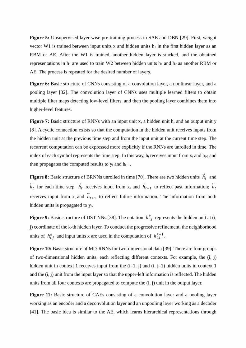
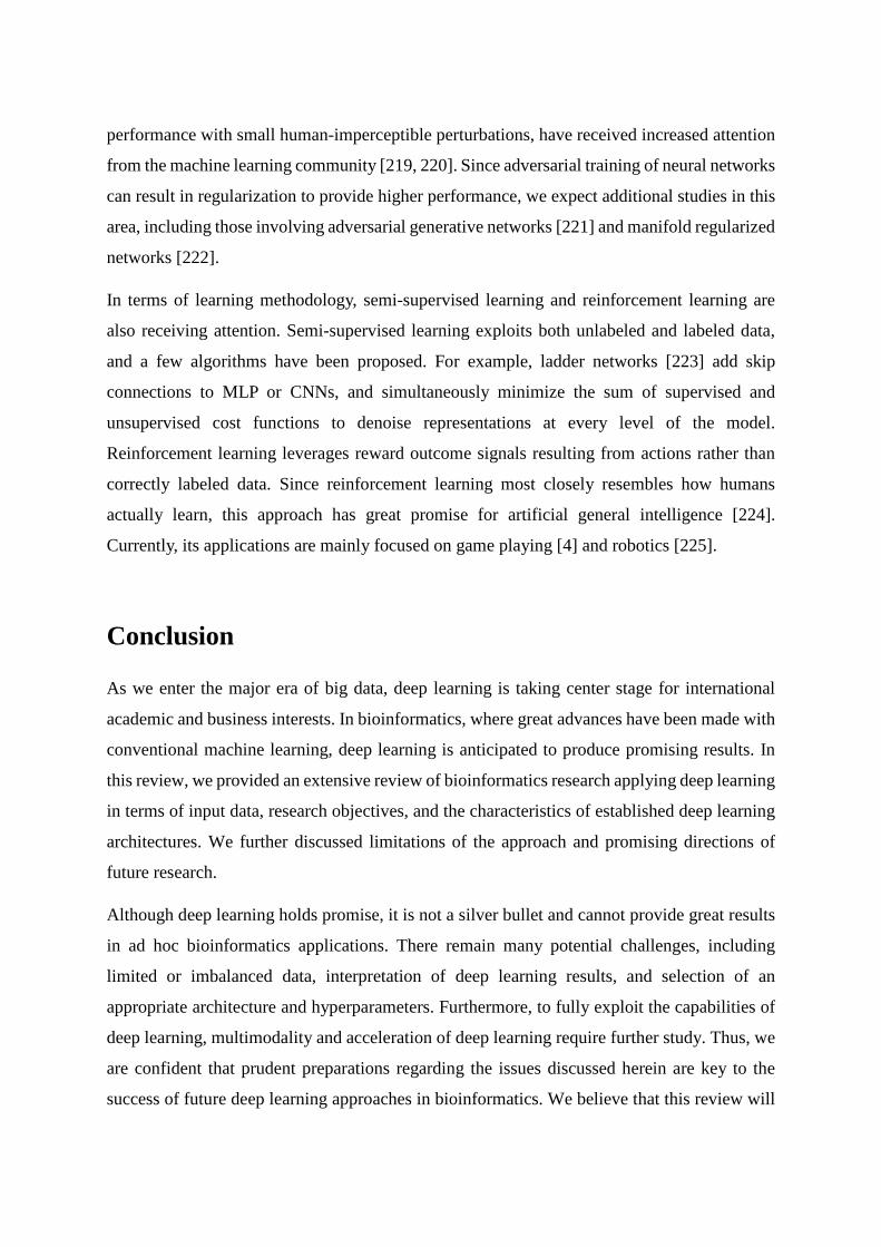
Figure 5: Unsupervised layer-wise pre-training process in SAE and DBN [29]. First, weight

vector W1 is trained between input units x and hidden units h1 in the first hidden layer as an

RBM or AE. After the W1 is trained, another hidden layer is stacked, and the obtained

representations in h1 are used to train W2 between hidden units h1 and h2 as another RBM or

AE. The process is repeated for the desired number of layers.

Figure 6: Basic structure of CNNs consisting of a convolution layer, a nonlinear layer, and a

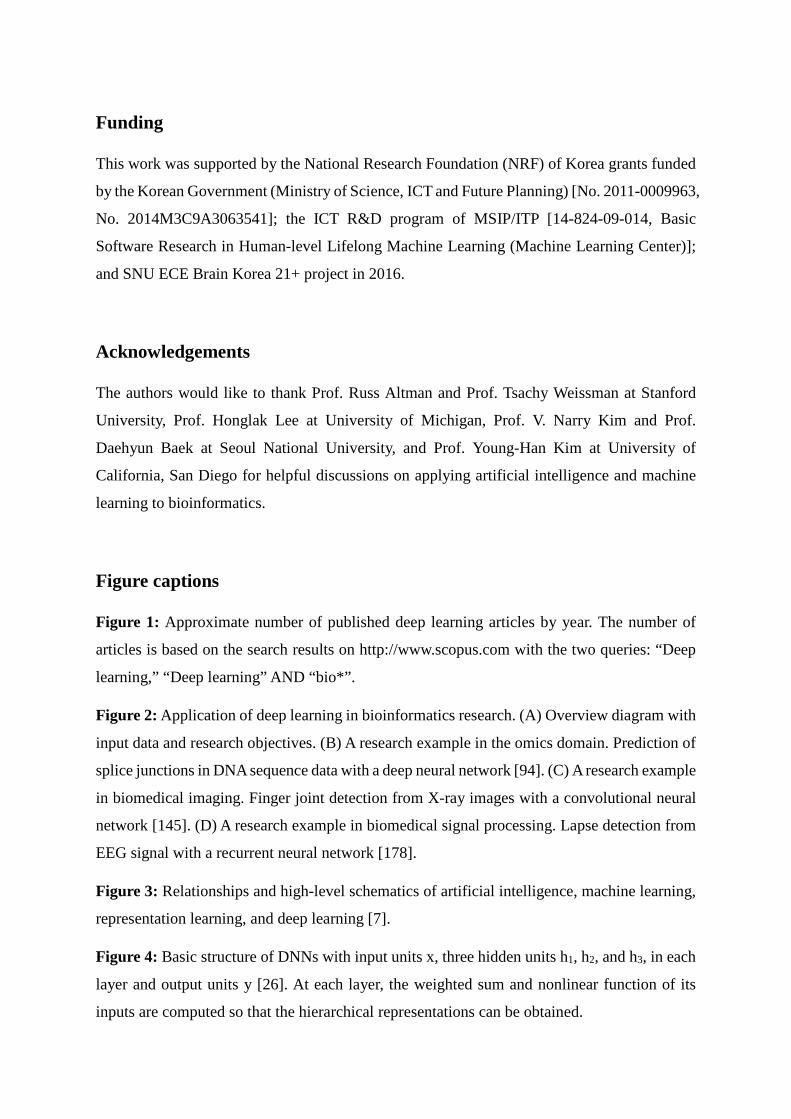
pooling layer [32]. The convolution layer of CNNs uses multiple learned filters to obtain

multiple filter maps detecting low-level filters, and then the pooling layer combines them into

higher-level features.

Figure 7: Basic structure of RNNs with an input unit x, a hidden unit h, and an output unit y

[8]. A cyclic connection exists so that the computation in the hidden unit receives inputs from

the hidden unit at the previous time step and from the input unit at the current time step. The

recurrent computation can be expressed more explicitly if the RNNs are unrolled in time. The

index of each symbol represents the time step. In this way, ht receives input from xt and ht-1 and

then propagates the computed results to yt and ht+1.

Figure 8: Basic structure of BRNNs unrolled in time [70]. There are two hidden units ℎ�⃗ 𝑡𝑡 and

ℎ⃖�𝑡𝑡 for each time step. ℎ�⃗ 𝑡𝑡 receives input from xt and ℎ�⃗ 𝑡𝑡−1 to reflect past information; ℎ⃖�𝑡𝑡

receives input from xt and ℎ⃖�𝑡𝑡+1 to reflect future information. The information from both

hidden units is propagated to yt.

Figure 9: Basic structure of DST-NNs [38]. The notation ℎ𝑖𝑖,𝑗𝑗𝑘𝑘 represents the hidden unit at (i,

j) coordinate of the k-th hidden layer. To conduct the progressive refinement, the neighborhood

units of ℎ𝑖𝑖,𝑗𝑗𝑘𝑘 and input units x are used in the computation of ℎ𝑖𝑖,𝑗𝑗𝑘𝑘+1.

Figure 10: Basic structure of MD-RNNs for two-dimensional data [39]. There are four groups

of two-dimensional hidden units, each reflecting different contexts. For example, the (i, j)

hidden unit in context 1 receives input from the (i–1, j) and (i, j–1) hidden units in context 1

and the (i, j) unit from the input layer so that the upper-left information is reflected. The hidden

units from all four contexts are propagated to compute the (i, j) unit in the output layer.

Figure 11: Basic structure of CAEs consisting of a convolution layer and a pooling layer

working as an encoder and a deconvolution layer and an unpooling layer working as a decoder

[41]. The basic idea is similar to the AE, which learns hierarchical representations through

reconstructing its input data, but CAE additionally utilizes spatial information by integrating

convolutions.

References

1. Manyika J, Chui M, Brown B et al. Big data: The next frontier for innovation, competition, and

productivity 2011.

2. Ferrucci D, Brown E, Chu-Carroll J et al. Building Watson: An overview of the DeepQA project.

AI magazine 2010;31(3):59-79.

3. IBM Watson for Oncology. IBM. http://www.ibm.com/smarterplanet/us/en/ibmwatson/watson-

oncology.html, 2016.

4. Silver D, Huang A, Maddison CJ et al. Mastering the game of Go with deep neural networks

and tree search. Nature 2016;529(7587):484-9.

5. DeepMind Health. Google DeepMind. https://www.deepmind.com/health, 2016.

6. Larrañaga P, Calvo B, Santana R et al. Machine learning in bioinformatics. Briefings in

bioinformatics 2006;7(1):86-112.

7. Goodfellow I, Bengio Y, Courville A. Deep Learning. Book in preparation for MIT Press, 2016.

8. LeCun Y, Bengio Y, Hinton G. Deep learning. Nature 2015;521(7553):436-44.

9. Farabet C, Couprie C, Najman L et al. Learning hierarchical features for scene labeling. Pattern

Analysis and Machine Intelligence, IEEE Transactions on 2013;35(8):1915-29.

10. Szegedy C, Liu W, Jia Y et al. Going deeper with convolutions. arXiv preprint arXiv:1409.4842

2014.

11. Tompson JJ, Jain A, LeCun Y et al. Joint training of a convolutional network and a graphical

model for human pose estimation. In: Advances in neural information processing systems. 2014. p.

1799-807.

12. Liu N, Han J, Zhang D et al. Predicting eye fixations using convolutional neural networks. In:

Proceedings of the IEEE Conference on Computer Vision and Pattern Recognition. 2015. p. 362-70.

13. Hinton G, Deng L, Yu D et al. Deep neural networks for acoustic modeling in speech recognition:

The shared views of four research groups. Signal Processing Magazine, IEEE 2012;29(6):82-97.

14. Sainath TN, Mohamed A-r, Kingsbury B et al. Deep convolutional neural networks for LVCSR. In:

Acoustics, Speech and Signal Processing (ICASSP), 2013 IEEE International Conference on. 2013. p.

8614-8. IEEE.

15. Chorowski JK, Bahdanau D, Serdyuk D et al. Attention-based models for speech recognition. In:

Advances in neural information processing systems. 2015. p. 577-85.

16. Kiros R, Zhu Y, Salakhutdinov RR et al. Skip-thought vectors. In: Advances in neural information

processing systems. 2015. p. 3276-84.

17. Li J, Luong M-T, Jurafsky D. A hierarchical neural autoencoder for paragraphs and documents.

arXiv preprint arXiv:1506.01057 2015.

18. Luong M-T, Pham H, Manning CD. Effective approaches to attention-based neural machine

translation. arXiv preprint arXiv:1508.04025 2015.

19. Cho K, Van Merriënboer B, Gulcehre C et al. Learning phrase representations using RNN

encoder-decoder for statistical machine translation. arXiv preprint arXiv:1406.1078 2014.

20. Libbrecht MW, Noble WS. Machine learning applications in genetics and genomics. Nature

Reviews Genetics 2015;16(6):321-32.

21. Schmidhuber J. Deep learning in neural networks: An overview. Neural networks 2015;61:85-

117.

22. Leung MK, Delong A, Alipanahi B et al. Machine Learning in Genomic Medicine: A Review of

Computational Problems and Data Sets 2016.

23. Mamoshina P, Vieira A, Putin E et al. Applications of deep learning in biomedicine. Molecular

Pharmaceutics 2016.

24. Greenspan H, van Ginneken B, Summers RM. Guest Editorial Deep Learning in Medical Imaging:

Overview and Future Promise of an Exciting New Technique. IEEE Transactions on Medical Imaging

2016;35(5):1153-9.

25. LeCun Y, Ranzato M. Deep learning tutorial. In: Tutorials in International Conference on Machine

Learning (ICML’13). 2013. Citeseer.

26. Svozil D, Kvasnicka V, Pospichal J. Introduction to multi-layer feed-forward neural networks.

Chemometrics and intelligent laboratory systems 1997;39(1):43-62.

27. Vincent P, Larochelle H, Bengio Y et al. Extracting and composing robust features with denoising

autoencoders. In: Proceedings of the 25th international conference on Machine learning. 2008. p.

1096-103. ACM.

28. Vincent P, Larochelle H, Lajoie I et al. Stacked denoising autoencoders: Learning useful

representations in a deep network with a local denoising criterion. The Journal of Machine Learning

Research 2010;11:3371-408.

29. Hinton G, Osindero S, Teh Y-W. A fast learning algorithm for deep belief nets. Neural

Computation 2006;18(7):1527-54.

30. Hinton G, Salakhutdinov RR. Reducing the dimensionality of data with neural networks. Science

2006;313(5786):504-7.

31. LeCun Y, Boser B, Denker JS et al. Handwritten digit recognition with a back-propagation

network. In: Advances in neural information processing systems. 1990. Citeseer.

32. Lawrence S, Giles CL, Tsoi AC et al. Face recognition: A convolutional neural-network approach.

Neural Networks, IEEE Transactions on 1997;8(1):98-113.

33. Krizhevsky A, Sutskever I, Hinton G. Imagenet classification with deep convolutional neural

networks. In: Advances in neural information processing systems. 2012. p. 1097-105.

34. Williams RJ, Zipser D. A learning algorithm for continually running fully recurrent neural

networks. Neural Computation 1989;1(2):270-80.

35. Bengio Y, Simard P, Frasconi P. Learning long-term dependencies with gradient descent is

difficult. Neural Networks, IEEE Transactions on 1994;5(2):157-66.

36. Hochreiter S, Schmidhuber J. Long short-term memory. Neural Computation 1997;9(8):1735-80.

37. Gers FA, Schmidhuber J, Cummins F. Learning to forget: Continual prediction with LSTM. Neural

Computation 2000;12(10):2451-71.

38. Lena PD, Nagata K, Baldi PF. Deep spatio-temporal architectures and learning for protein

structure prediction. In: Advances in neural information processing systems. 2012. p. 512-20.

39. Graves A, Schmidhuber J. Offline handwriting recognition with multidimensional recurrent

neural networks. In: Advances in neural information processing systems. 2009. p. 545-52.

40. Hadsell R, Sermanet P, Ben J et al. Learning long‐range vision for autonomous off‐road driving.

Journal of Field Robotics 2009;26(2):120-44.

41. Masci J, Meier U, Cireşan D et al. Stacked convolutional auto-encoders for hierarchical feature

extraction. Artificial Neural Networks and Machine Learning–ICANN 2011. Springer, 2011, 52-9.

42. Minsky M, Papert S. Perceptron: an introduction to computational geometry. The MIT Press,

Cambridge, expanded edition 1969;19(88):2.

43. Fukushima K. Cognitron: A self-organizing multilayered neural network. Biological cybernetics

1975;20(3-4):121-36.

44. Hinton G, Sejnowski TJ. Learning and releaming in Boltzmann machines. Parallel distributed

processing: Explorations in the microstructure of cognition 1986;1:282-317.

45. Hinton G. A practical guide to training restricted Boltzmann machines. Momentum 2010;9(1):926.

46. Hecht-Nielsen R. Theory of the backpropagation neural network. In: Neural Networks, 1989.

IJCNN., International Joint Conference on. 1989. p. 593-605. IEEE.

47. Bottou L. Stochastic gradient learning in neural networks. Proceedings of Neuro-Nımes

1991;91(8).

48. Duchi J, Hazan E, Singer Y. Adaptive subgradient methods for online learning and stochastic

optimization. The Journal of Machine Learning Research 2011;12:2121-59.

49. Kingma D, Ba J. Adam: A method for stochastic optimization. arXiv preprint arXiv:1412.6980

2014.

50. Moody J, Hanson S, Krogh A et al. A simple weight decay can improve generalization. Advances

in neural information processing systems 1995;4:950-7.

51. Srivastava N, Hinton G, Krizhevsky A et al. Dropout: A simple way to prevent neural networks

from overfitting. The Journal of Machine Learning Research 2014;15(1):1929-58.

52. Baldi P, Sadowski PJ. Understanding dropout. In: Advances in neural information processing

systems. 2013. p. 2814-22.

53. Goodfellow IJ, Warde-Farley D, Mirza M et al. Maxout networks. arXiv preprint arXiv:1302.4389

2013.

54. Moon T, Choi H, Lee H et al. RnnDrop: A Novel Dropout for RNNs in ASR. Automatic Speech

Recognition and Understanding (ASRU) 2015.

55. Ioffe S, Szegedy C. Batch normalization: Accelerating deep network training by reducing internal

covariate shift. arXiv preprint arXiv:1502.03167 2015.

56. Deeplearning4j Development Team. Deeplearning4j: Open-source distributed deep learning for

the JVM. Apache Software Foundation License 2.0. http://deeplearning4j.org, 2016.

57. Bahrampour S, Ramakrishnan N, Schott L et al. Comparative Study of Deep Learning Software

Frameworks. arXiv preprint arXiv:1511.06435 2015.

58. Nervana Systems. Neon. https://github.com/NervanaSystems/neon, 2016.

59. Jia Y. Caffe: An open source convolutional architecture for fast feature embedding. In: ACM

International Conference on Multimedia. ACM. 2014.

60. Collobert R, Kavukcuoglu K, Farabet C. Torch7: A matlab-like environment for machine learning.

In: BigLearn, NIPS Workshop. 2011.

61. Bergstra J, Breuleux O, Bastien F et al. Theano: a CPU and GPU math expression compiler. In:

Proceedings of the Python for scientific computing conference (SciPy). 2010. p. 3. Austin, TX.

62. Bastien F, Lamblin P, Pascanu R et al. Theano: new features and speed improvements. arXiv

preprint arXiv:1211.5590 2012.

63. Chollet F. Keras: Theano-based Deep Learning library. Code: https://github. com/fchollet.

Documentation: http://keras. io 2015.

64. Dieleman S, Heilman M, Kelly J et al. Lasagne: First release 2015.

65. van Merriënboer B, Bahdanau D, Dumoulin V et al. Blocks and fuel: Frameworks for deep

learning. arXiv preprint arXiv:1506.00619 2015.

66. Abadi M, Agarwal A, Barham P et al. TensorFlow: Large-Scale Machine Learning on

Heterogeneous Distributed Systems. arXiv preprint arXiv:1603.04467 2016.

67. Nair V, Hinton G. Rectified linear units improve restricted boltzmann machines. In: Proceedings

of the 27th International Conference on Machine Learning (ICML-10). 2010. p. 807-14.

68. Erhan D, Bengio Y, Courville A et al. Why does unsupervised pre-training help deep learning?

The Journal of Machine Learning Research 2010;11:625-60.

69. Hubel DH, Wiesel TN. Receptive fields and functional architecture of monkey striate cortex. The

Journal of physiology 1968;195(1):215-43.

70. Schuster M, Paliwal KK. Bidirectional recurrent neural networks. Signal Processing, IEEE

Transactions on 1997;45(11):2673-81.

71. Cenic A, Nabavi DG, Craen RA et al. Dynamic CT measurement of cerebral blood flow: a

validation study. American Journal of Neuroradiology 1999;20(1):63-73.

72. Tsao J, Boesiger P, Pruessmann KP. k‐t BLAST and k‐t SENSE: Dynamic MRI with high frame rate

exploiting spatiotemporal correlations. Magnetic Resonance in Medicine 2003;50(5):1031-42.

73. Cohen AM, Hersh WR. A survey of current work in biomedical text mining. Briefings in

bioinformatics 2005;6(1):57-71.

74. Bahdanau D, Cho K, Bengio Y. Neural machine translation by jointly learning to align and

translate. arXiv preprint arXiv:1409.0473 2014.

75. Xu K, Ba J, Kiros R et al. Show, attend and tell: Neural image caption generation with visual

attention. arXiv preprint arXiv:1502.03044 2015.

76. Cho K, Courville A, Bengio Y. Describing multimedia content using attention-based encoder-

decoder networks. Multimedia, IEEE Transactions on 2015;17(11):1875-86.

77. Mnih V, Heess N, Graves A. Recurrent models of visual attention. In: Advances in neural

information processing systems. 2014. p. 2204-12.

78. Jones DT. Protein secondary structure prediction based on position-specific scoring matrices.

Journal of molecular biology 1999;292(2):195-202.

79. Ponomarenko JV, Ponomarenko MP, Frolov AS et al. Conformational and physicochemical DNA

features specific for transcription factor binding sites. Bioinformatics 1999;15(7):654-68.

80. Cai Y-d, Lin SL. Support vector machines for predicting rRNA-, RNA-, and DNA-binding proteins

from amino acid sequence. Biochimica et Biophysica Acta (BBA)-Proteins and Proteomics

2003;1648(1):127-33.

81. Atchley WR, Zhao J, Fernandes AD et al. Solving the protein sequence metric problem.

Proceedings of the National Academy of Sciences of the United States of America

2005;102(18):6395-400.

82. Branden CI. Introduction to protein structure. Garland Science, 1999.

83. Richardson JS. The anatomy and taxonomy of protein structure. Advances in protein chemistry

1981;34:167-339.

84. Lyons J, Dehzangi A, Heffernan R et al. Predicting backbone Cα angles and dihedrals from

protein sequences by stacked sparse auto‐encoder deep neural network. Journal of computational

chemistry 2014;35(28):2040-6.

85. Heffernan R, Paliwal K, Lyons J et al. Improving prediction of secondary structure, local backbone

angles, and solvent accessible surface area of proteins by iterative deep learning. Scientific reports

2015;5.

86. Spencer M, Eickholt J, Cheng J. A Deep Learning Network Approach to ab initio Protein

Secondary Structure Prediction. Computational Biology and Bioinformatics, IEEE/ACM Transactions

on 2015;12(1):103-12.

87. Nguyen SP, Shang Y, Xu D. DL-PRO: A novel deep learning method for protein model quality

assessment. In: Neural Networks (IJCNN), 2014 International Joint Conference on. 2014. p. 2071-8.

IEEE.

88. Baldi P, Brunak S, Frasconi P et al. Exploiting the past and the future in protein secondary

structure prediction. Bioinformatics 1999;15(11):937-46.

89. Baldi P, Pollastri G, Andersen CA et al. Matching protein beta-sheet partners by feedforward

and recurrent neural networks. In: Proceedings of the 2000 Conference on Intelligent Systems for

Molecular Biology (ISMB00), La Jolla, CA. 2000. p. 25-36.

90. Sønderby SK, Winther O. Protein Secondary Structure Prediction with Long Short Term Memory

Networks. arXiv preprint arXiv:1412.7828 2014.

91. Lena PD, Nagata K, Baldi P. Deep architectures for protein contact map prediction. Bioinformatics

2012;28(19):2449-57.

92. Baldi P, Pollastri G. The principled design of large-scale recursive neural network architectures-

-dag-rnns and the protein structure prediction problem. The Journal of Machine Learning Research

2003;4:575-602.

93. Leung MK, Xiong HY, Lee LJ et al. Deep learning of the tissue-regulated splicing code.

Bioinformatics 2014;30(12):i121-i9.

94. Lee T, Yoon S. Boosted Categorical Restricted Boltzmann Machine for Computational Prediction

of Splice Junctions. In: International Conference on Machine Learning. Lille, France, 2015. p. 2483–

92.

95. Zhang S, Zhou J, Hu H et al. A deep learning framework for modeling structural features of

RNA-binding protein targets. Nucleic acids research 2015:gkv1025.

96. Chen Y, Li Y, Narayan R et al. Gene expression inference with deep learning. Bioinformatics

2016(btw074).

97. Li Y, Shi W, Wasserman WW. Genome-Wide Prediction of cis-Regulatory Regions Using

Supervised Deep Learning Methods. bioRxiv 2016:041616.

98. Liu F, Ren C, Li H et al. De novo identification of replication-timing domains in the human

genome by deep learning. Bioinformatics 2015:btv643.

99. Denas O, Taylor J. Deep modeling of gene expression regulation in an Erythropoiesis model. In:

International Conference on Machine Learning workshop on Representation Learning. Atlanta,

Georgia, USA, 2013.

100. Alipanahi B, Delong A, Weirauch MT et al. Predicting the sequence specificities of DNA-and

RNA-binding proteins by deep learning. Nature biotechnology 2015.

101. Lanchantin J, Singh R, Lin Z et al. Deep motif: Visualizing genomic sequence classifications. arXiv

preprint arXiv:1605.01133 2016.

102. Zeng H, Edwards MD, Liu G et al. Convolutional neural network architectures for predicting

DNA–protein binding. Bioinformatics 2016;32(12):i121-i7.

103. Kelley DR, Snoek J, Rinn J. Basset: Learning the regulatory code of the accessible genome with

deep convolutional neural networks. bioRxiv 2015:028399.

104. Zhou J, Troyanskaya OG. Predicting effects of noncoding variants with deep learning-based

sequence model. Nature methods 2015;12(10):931-4.

105. Park S, Min S, Choi H-s et al. deepMiRGene: Deep Neural Network based Precursor microRNA

Prediction. arXiv preprint arXiv:1605.00017 2016.

106. Lee B, Lee T, Na B et al. DNA-Level Splice Junction Prediction using Deep Recurrent Neural

Networks. arXiv preprint arXiv:1512.05135 2015.

107. Lee B, Baek J, Park S et al. deepTarget: End-to-end Learning Framework for microRNA Target

Prediction using Deep Recurrent Neural Networks. arXiv preprint arXiv:1603.09123 2016.

108. Asgari E, Mofrad MR. Continuous Distributed Representation of Biological Sequences for Deep

Proteomics and Genomics. PloS one 2015;10(11):e0141287.

109. Hochreiter S, Heusel M, Obermayer K. Fast model-based protein homology detection without

alignment. Bioinformatics 2007;23(14):1728-36.

110. Sønderby SK, Sønderby CK, Nielsen H et al. Convolutional LSTM Networks for Subcellular

Localization of Proteins. arXiv preprint arXiv:1503.01919 2015.

111. Fakoor R, Ladhak F, Nazi A et al. Using deep learning to enhance cancer diagnosis and

classification. In: Proceedings of the International Conference on Machine Learning. 2013.

112. Nilsen TW, Graveley BR. Expansion of the eukaryotic proteome by alternative splicing. Nature

2010;463(7280):457-63.

113. Jolliffe I. Principal component analysis. Wiley Online Library, 2002.

114. Park Y, Kellis M. Deep learning for regulatory genomics. Nature biotechnology 2015;33(8):825-

6.

115. Najarian K, Splinter R. Biomedical signal and image processing. CRC press, 2005.

116. Edelman RR, Warach S. Magnetic resonance imaging. New England Journal of Medicine

1993;328(10):708-16.

117. Ogawa S, Lee T-M, Kay AR et al. Brain magnetic resonance imaging with contrast dependent

on blood oxygenation. Proceedings of the National Academy of Sciences 1990;87(24):9868-72.

118. Hsieh J. Computed tomography: principles, design, artifacts, and recent advances. SPIE

Bellingham, WA, 2009.

119. Chapman D, Thomlinson W, Johnston R et al. Diffraction enhanced x-ray imaging. Physics in

medicine and biology 1997;42(11):2015.

120. Bailey DL, Townsend DW, Valk PE et al. Positron emission tomography. Springer, 2005.

121. Gurcan MN, Boucheron LE, Can A et al. Histopathological image analysis: a review. Biomedical

Engineering, IEEE Reviews in 2009;2:147-71.

122. Plis SM, Hjelm DR, Salakhutdinov R et al. Deep learning for neuroimaging: a validation study.

Frontiers in neuroscience 2014;8.

123. Hua K-L, Hsu C-H, Hidayati SC et al. Computer-aided classification of lung nodules on computed

tomography images via deep learning technique. OncoTargets and therapy 2015;8.

124. Suk H-I, Shen D. Deep learning-based feature representation for AD/MCI classification. Medical

Image Computing and Computer-Assisted Intervention–MICCAI 2013. Springer, 2013, 583-90.

125. Roth HR, Lu L, Liu J et al. Improving Computer-aided Detection using Convolutional Neural

Networks and Random View Aggregation. arXiv preprint arXiv:1505.03046 2015.

126. Roth HR, Yao J, Lu L et al. Detection of sclerotic spine metastases via random aggregation of

deep convolutional neural network classifications. Recent Advances in Computational Methods and

Clinical Applications for Spine Imaging. Springer, 2015, 3-12.

127. Li Q, Cai W, Wang X et al. Medical image classification with convolutional neural network. In:

Control Automation Robotics & Vision (ICARCV), 2014 13th International Conference on. 2014. p.

844-8. IEEE.

128. Cireşan DC, Giusti A, Gambardella LM et al. Mitosis detection in breast cancer histology images

with deep neural networks. Medical Image Computing and Computer-Assisted Intervention–

MICCAI 2013. Springer, 2013, 411-8.

129. Ypsilantis P-P, Siddique M, Sohn H-M et al. Predicting Response to Neoadjuvant Chemotherapy

with PET Imaging Using Convolutional Neural Networks. PloS one 2015;10(9):e0137036.

130. Zeng T, Li R, Mukkamala R et al. Deep convolutional neural networks for annotating gene

expression patterns in the mouse brain. BMC bioinformatics 2015;16(1):1-10.

131. Cruz-Roa AA, Ovalle JEA, Madabhushi A et al. A deep learning architecture for image

representation, visual interpretability and automated basal-cell carcinoma cancer detection.

Medical Image Computing and Computer-Assisted Intervention–MICCAI 2013. Springer, 2013, 403-

10.

132. Bar Y, Diamant I, Wolf L et al. Deep learning with non-medical training used for chest pathology

identification. In: SPIE Medical Imaging. 2015. p. 94140V-V-7. International Society for Optics and

Photonics.

133. Li Q, Feng B, Xie L et al. A Cross-modality Learning Approach for Vessel Segmentation in Retinal

Images. IEEE Transactions on Medical Imaging 2015;35(1):109 - 8.

134. Ning F, Delhomme D, LeCun Y et al. Toward automatic phenotyping of developing embryos

from videos. Image Processing, IEEE Transactions on 2005;14(9):1360-71.

135. Turaga SC, Murray JF, Jain V et al. Convolutional networks can learn to generate affinity graphs

for image segmentation. Neural Computation 2010;22(2):511-38.

136. Helmstaedter M, Briggman KL, Turaga SC et al. Connectomic reconstruction of the inner

plexiform layer in the mouse retina. Nature 2013;500(7461):168-74.

137. Ciresan D, Giusti A, Gambardella LM et al. Deep neural networks segment neuronal membranes

in electron microscopy images. In: Advances in neural information processing systems. 2012. p.

2843-51.

138. Prasoon A, Petersen K, Igel C et al. Deep feature learning for knee cartilage segmentation using

a triplanar convolutional neural network. Medical Image Computing and Computer-Assisted

Intervention–MICCAI 2013. Springer, 2013, 246-53.

139. Havaei M, Davy A, Warde-Farley D et al. Brain Tumor Segmentation with Deep Neural Networks.

arXiv preprint arXiv:1505.03540 2015.

140. Roth HR, Lu L, Farag A et al. Deeporgan: Multi-level deep convolutional networks for automated

pancreas segmentation. Medical Image Computing and Computer-Assisted Intervention–MICCAI

2015. Springer, 2015, 556-64.

141. Stollenga MF, Byeon W, Liwicki M et al. Parallel Multi-Dimensional LSTM, With Application to

Fast Biomedical Volumetric Image Segmentation. arXiv preprint arXiv:1506.07452 2015.

142. Xu J, Xiang L, Liu Q et al. Stacked Sparse Autoencoder (SSAE) for Nuclei Detection on Breast

Cancer Histopathology images. IEEE Transactions on Medical Imaging 2015;35(1):119 - 30.

143. Chen CL, Mahjoubfar A, Tai L-C et al. Deep Learning in Label-free Cell Classification. Scientific

reports 2016;6.

144. Cho J, Lee K, Shin E et al. Medical Image Deep Learning with Hospital PACS Dataset. arXiv

preprint arXiv:1511.06348 2015.

145. Lee S, Choi M, Choi H-s et al. FingerNet: Deep learning-based robust finger joint detection

from radiographs. In: Biomedical Circuits and Systems Conference (BioCAS), 2015 IEEE. 2015. p. 1-4.

IEEE.

146. Roth HR, Lee CT, Shin H-C et al. Anatomy-specific classification of medical images using deep

convolutional nets. arXiv preprint arXiv:1504.04003 2015.

147. Roth HR, Lu L, Seff A et al. A new 2.5 D representation for lymph node detection using random

sets of deep convolutional neural network observations. Medical Image Computing and Computer-

Assisted Intervention–MICCAI 2014. Springer, 2014, 520-7.

148. Kraus OZ, Frey BJ. Computer vision for high content screening. Critical reviews in biochemistry

and molecular biology 2016;51(2):102-9.

149. Gerven MAV, De Lange FP, Heskes T. Neural decoding with hierarchical generative models.

Neural Computation 2010;22(12):3127-42.

150. Koyamada S, Shikauchi Y, Nakae K et al. Deep learning of fMRI big data: a novel approach to

subject-transfer decoding. arXiv preprint arXiv:1502.00093 2015.

151. Duryea J, Jiang Y, Countryman P et al. Automated algorithm for the identification of joint space

and phalanx margin locations on digitized hand radiographs. Medical Physics 1999;26(3):453-61.

152. Niedermeyer E, da Silva FL. Electroencephalography: basic principles, clinical applications, and

related fields. Lippincott Williams & Wilkins, 2005.

153. Buzsáki G, Anastassiou CA, Koch C. The origin of extracellular fields and currents—EEG, ECoG,

LFP and spikes. Nature reviews neuroscience 2012;13(6):407-20.

154. Marriott HJL, Wagner GS. Practical electrocardiography. Williams & Wilkins Baltimore, 1988.

155. De Luca CJ. The use of surface electromyography in biomechanics. Journal of applied

biomechanics 1997;13:135-63.

156. Young LR, Sheena D. Eye-movement measurement techniques. American Psychologist

1975;30(3):315.

157. Barea R, Boquete L, Mazo M et al. System for assisted mobility using eye movements based on

electrooculography. Neural Systems and Rehabilitation Engineering, IEEE Transactions on

2002;10(4):209-18.

158. Freudenburg ZV, Ramsey NF, Wronkeiwicz M et al. Real-time naive learning of neural correlates

in ECoG Electrophysiology. Int. Journal of Machine Learning and Computing 2011.

159. An X, Kuang D, Guo X et al. A Deep Learning Method for Classification of EEG Data Based on

Motor Imagery. Intelligent Computing in Bioinformatics. Springer, 2014, 203-10.

160. Li K, Li X, Zhang Y et al. Affective state recognition from EEG with deep belief networks. In:

Bioinformatics and Biomedicine (BIBM), 2013 IEEE International Conference on. 2013. p. 305-10. IEEE.

161. Jia X, Li K, Li X et al. A Novel Semi-Supervised Deep Learning Framework for Affective State

Recognition on EEG Signals. In: Bioinformatics and Bioengineering (BIBE), 2014 IEEE International

Conference on. 2014. p. 30-7. IEEE.

162. Zheng W-L, Guo H-T, Lu B-L. Revealing critical channels and frequency bands for emotion

recognition from EEG with deep belief network. In: Neural Engineering (NER), 2015 7th International

IEEE/EMBS Conference on. 2015. p. 154-7. IEEE.

163. Jirayucharoensak S, Pan-Ngum S, Israsena P. EEG-based emotion recognition using deep

learning network with principal component based covariate shift adaptation. The Scientific World

Journal 2014;2014.

164. Stober S, Cameron DJ, Grahn JA. Classifying EEG recordings of rhythm perception. In: 15th

International Society for Music Information Retrieval Conference (ISMIR’14). 2014. p. 649-54.

165. Stober S, Cameron DJ, Grahn JA. Using Convolutional Neural Networks to Recognize Rhythm.

In: Advances in neural information processing systems. 2014. p. 1449-57.

166. Cecotti H, Graeser A. Convolutional neural network with embedded Fourier transform for EEG

classification. In: Pattern Recognition, 2008. ICPR 2008. 19th International Conference on. 2008. p.

1-4. IEEE.

167. Cecotti H, Gräser A. Convolutional neural networks for P300 detection with application to brain-

computer interfaces. Pattern Analysis and Machine Intelligence, IEEE Transactions on 2011;33(3):433-

45.

168. Soleymani M, Asghari-Esfeden S, Pantic M et al. Continuous emotion detection using EEG

signals and facial expressions. In: Multimedia and Expo (ICME), 2014 IEEE International Conference

on. 2014. p. 1-6. IEEE.

169. Wang Z, Lyu S, Schalk G et al. Deep feature learning using target priors with applications in

ECoG signal decoding for BCI. In: Proceedings of the Twenty-Third international joint conference on

Artificial Intelligence. 2013. p. 1785-91. AAAI Press.

170. Stober S, Sternin A, Owen AM et al. Deep Feature Learning for EEG Recordings. arXiv preprint

arXiv:1511.04306 2015.

171. Huanhuan M, Yue Z. Classification of Electrocardiogram Signals with Deep Belief Networks. In:

Computational Science and Engineering (CSE), 2014 IEEE 17th International Conference on. 2014. p.

7-12. IEEE.

172. Wulsin D, Gupta J, Mani R et al. Modeling electroencephalography waveforms with semi-

supervised deep belief nets: fast classification and anomaly measurement. Journal of neural

engineering 2011;8(3):036015.

173. Turner J, Page A, Mohsenin T et al. Deep belief networks used on high resolution multichannel

electroencephalography data for seizure detection. In: 2014 AAAI Spring Symposium Series. 2014.

174. Zhao Y, He L. Deep Learning in the EEG Diagnosis of Alzheimer’s Disease. In: Computer Vision-

ACCV 2014 Workshops. 2014. p. 340-53. Springer.

175. Längkvist M, Karlsson L, Loutfi A. Sleep stage classification using unsupervised feature learning.

Advances in Artificial Neural Systems 2012;2012:5.

176. Mirowski P, Madhavan D, LeCun Y et al. Classification of patterns of EEG synchronization for

seizure prediction. Clinical neurophysiology 2009;120(11):1927-40.

177. Petrosian A, Prokhorov D, Homan R et al. Recurrent neural network based prediction of epileptic

seizures in intra-and extracranial EEG. Neurocomputing 2000;30(1):201-18.

178. Davidson PR, Jones RD, Peiris MT. EEG-based lapse detection with high temporal resolution.

Biomedical Engineering, IEEE Transactions on 2007;54(5):832-9.

179. Oh S, Lee MS, Zhang B-T. Ensemble learning with active example selection for imbalanced

biomedical data classification. IEEE/ACM Transactions on Computational Biology and Bioinformatics

(TCBB) 2011;8(2):316-25.

180. Malin BA, El Emam K, O'Keefe CM. Biomedical data privacy: problems, perspectives, and recent

advances. Journal of the American medical informatics association 2013;20(1):2-6.

181. He H, Garcia EA. Learning from imbalanced data. Knowledge and Data Engineering, IEEE

Transactions on 2009;21(9):1263-84.

182. Davis J, Goadrich M. The relationship between Precision-Recall and ROC curves. In: Proceedings

of the 23rd international conference on Machine learning. 2006. p. 233-40. ACM.

183. López V, Fernández A, García S et al. An insight into classification with imbalanced data:

Empirical results and current trends on using data intrinsic characteristics. Information Sciences

2013;250:113-41.

184. Liu X-Y, Wu J, Zhou Z-H. Exploratory undersampling for class-imbalance learning. Systems, Man,

and Cybernetics, Part B: Cybernetics, IEEE Transactions on 2009;39(2):539-50.

185. Chawla NV, Bowyer KW, Hall LO et al. SMOTE: synthetic minority over-sampling technique.

Journal of artificial intelligence research 2002:321-57.

186. Jo T, Japkowicz N. Class imbalances versus small disjuncts. ACM Sigkdd Explorations Newsletter

2004;6(1):40-9.

187. Kukar M, Kononenko I. Cost-Sensitive Learning with Neural Networks. In: ECAI. 1998. p. 445-9.

Citeseer.

188. Pan SJ, Yang Q. A survey on transfer learning. Knowledge and Data Engineering, IEEE

Transactions on 2010;22(10):1345-59.

189. Deng J, Dong W, Socher R et al. Imagenet: A large-scale hierarchical image database. In:

Computer Vision and Pattern Recognition, 2009. CVPR 2009. IEEE Conference on. 2009. p. 248-55.

IEEE.

190. Zeiler MD, Fergus R. Visualizing and understanding convolutional networks. Computer Vision–

ECCV 2014. Springer, 2014, 818-33.

191. Erhan D, Bengio Y, Courville A et al. Visualizing higher-layer features of a deep network.

University of Montreal 2009;1341.

192. Simonyan K, Vedaldi A, Zisserman A. Deep inside convolutional networks: Visualising image

classification models and saliency maps. arXiv preprint arXiv:1312.6034 2013.

193. Choromanska A, Henaff M, Mathieu M et al. The loss surfaces of multilayer networks. arXiv

preprint arXiv:1412.0233 2014.

194. Dauphin YN, Pascanu R, Gulcehre C et al. Identifying and attacking the saddle point problem

in high-dimensional non-convex optimization. In: Advances in neural information processing

systems. 2014. p. 2933-41.

195. Bengio Y. Practical recommendations for gradient-based training of deep architectures. Neural

Networks: Tricks of the Trade. Springer, 2012, 437-78.

196. Bergstra J, Bardenet R, Bengio Y et al. Algorithms for hyper-parameter optimization. In: Advances

in neural information processing systems. 2011. p. 2546-54.

197. Hutter F, Hoos HH, Leyton-Brown K. Sequential model-based optimization for general algorithm

configuration. Learning and Intelligent Optimization. Springer, 2011, 507-23.

198. Snoek J, Larochelle H, Adams RP. Practical bayesian optimization of machine learning algorithms.

In: Advances in neural information processing systems. 2012. p. 2951-9.

199. Bergstra J, Bengio Y. Random search for hyper-parameter optimization. The Journal of Machine

Learning Research 2012;13(1):281-305.

200. Ngiam J, Khosla A, Kim M et al. Multimodal deep learning. In: Proceedings of the 28th

international conference on machine learning (ICML-11). 2011. p. 689-96.

201. Cao Y, Steffey S, He J et al. Medical Image Retrieval: A Multimodal Approach. Cancer informatics

2014;13(Suppl 3):125.

202. Ngiam J, Coates A, Lahiri A et al. On optimization methods for deep learning. In: Proceedings

of the 28th International Conference on Machine Learning (ICML-11). 2011. p. 265-72.

203. Martens J. Deep learning via Hessian-free optimization. In: Proceedings of the 27th International

Conference on Machine Learning (ICML-10). 2010. p. 735-42.

204. Raina R, Madhavan A, Ng AY. Large-scale deep unsupervised learning using graphics processors.

In: Proceedings of the 26th annual international conference on machine learning. 2009. p. 873-80.

ACM.

205. Ho Q, Cipar J, Cui H et al. More effective distributed ml via a stale synchronous parallel

parameter server. In: Advances in neural information processing systems. 2013. p. 1223-31.

206. Bengio Y, Schwenk H, Senécal J-S et al. Neural probabilistic language models. Innovations in

Machine Learning. Springer, 2006, 137-86.

207. Li M, Andersen DG, Park JW et al. Scaling distributed machine learning with the parameter

server. In: 11th USENIX Symposium on Operating Systems Design and Implementation (OSDI 14).

2014. p. 583-98.

208. Dean J, Corrado G, Monga R et al. Large scale distributed deep networks. In: Advances in neural

information processing systems. 2012. p. 1223-31.

209. Kin H, Park J, Jang J et al. DeepSpark: Spark-Based Deep Learning Supporting Asynchronous

Updates and Caffe Compatibility. arXiv preprint arXiv:1602.08191 2016.

210. Abadi M, Agarwal A, Barham P et al. TensorFlow: Large-scale machine learning on

heterogeneous systems, 2015. Software available from tensorflow. org 2015.

211. Simonite T. Thinking in Silicon. MIT Technology Review, 2013.

212. Ovtcharov K, Ruwase O, Kim J-Y et al. Accelerating deep convolutional neural networks using

specialized hardware. Microsoft Research Whitepaper 2015;2.

213. Farabet C, Poulet C, Han JY et al. Cnp: An fpga-based processor for convolutional networks. In:

Field Programmable Logic and Applications, 2009. FPL 2009. International Conference on. 2009. p.

32-7. IEEE.

214. Hof RD. Neuromorphic Chips. MIT Technology Review, 2014.

215. Yao L, Torabi A, Cho K et al. Describing videos by exploiting temporal structure. In: Proceedings

of the IEEE International Conference on Computer Vision. 2015. p. 4507-15.

216. Noh H, Seo PH, Han B. Image Question Answering using Convolutional Neural Network with

Dynamic Parameter Prediction. arXiv preprint arXiv:1511.05756 2015.

217. Graves A, Wayne G, Danihelka I. Neural turing machines. arXiv preprint arXiv:1410.5401 2014.

218. Weston J, Chopra S, Bordes A. Memory networks. arXiv preprint arXiv:1410.3916 2014.

219. Szegedy C, Zaremba W, Sutskever I et al. Intriguing properties of neural networks. arXiv preprint

arXiv:1312.6199 2013.

220. Goodfellow IJ, Shlens J, Szegedy C. Explaining and harnessing adversarial examples. arXiv

preprint arXiv:1412.6572 2014.

221. Goodfellow I, Pouget-Abadie J, Mirza M et al. Generative adversarial nets. In: Advances in neural

information processing systems. 2014. p. 2672-80.

222. Lee T, Choi M, Yoon S. Manifold Regularized Deep Neural Networks using Adversarial Examples.

arXiv preprint arXiv:1511.06381 2015.

223. Rasmus A, Berglund M, Honkala M et al. Semi-Supervised Learning with Ladder Networks. In:

Advances in neural information processing systems. 2015. p. 3532-40.

224. Arel I. Deep Reinforcement Learning as Foundation for Artificial General Intelligence.

Theoretical Foundations of Artificial General Intelligence. Springer, 2012, 89-102.

225. Cutler M, How JP. Efficient reinforcement learning for robots using informative simulated priors.

In: Robotics and Automation (ICRA), 2015 IEEE International Conference on. 2015. p. 2605-12. IEEE.