Embed Size (px)
Citation preview

Deep Learning for Vision
Marc'Aurelio Ranzato
Facebook, AI Group
Berkeley – 24 Jansuary 2014www.cs.toronto.edu/~ranzato

2
fixed unsupervised supervised
classifierMixture ofGaussians
MFCC \ˈd ē p\
fixed unsupervised supervised
classifierK-Means/poolingSIFT/HOG “car”
fixed unsupervised supervised
classifiern-gramsParse TreeSyntactic “+”
This burrito placeis yummy and fun!
Traditional Pattern Recognition
VISION
SPEECH
NLP
Ranzato
3
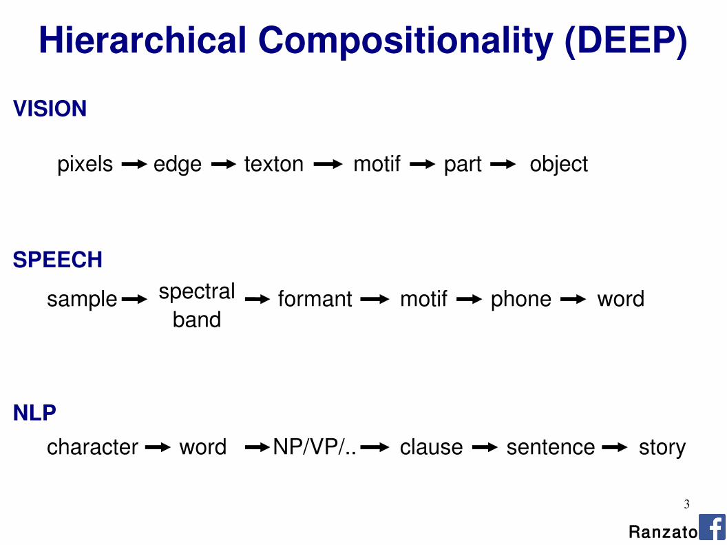
Hierarchical Compositionality (DEEP)
VISION
SPEECH
NLP
pixels edge texton motif part object
sample spectral band
formant motif phone word
character NP/VP/.. clause sentence storyword
Ranzato

4
Deep Learning
“car”
Cascade of non-linear transformations End to end learning General framework (any hierarchical model is deep)
What is Deep Learning
Ranzato

5
Deep Learning VS Shallow Learning
Structure of the system naturally matches the problem which is inherently hierarchical.
pixels edge texton motif part object
Ranzato

6
Deep Learning
“car”
Zeiler et al. “Visualizing and Understanding ConvNets” Arxiv 2013 Ranzato

7
Deep Learning VS Shallow Learning
Structure of the system naturally matches the problem which is inherently hierarchical.
It is more efficient.
E.g.: Checking N-bit parity requires N-1 gates laid out on a tree of depth log(N-1). The same would require O(exp(N)) with a two layer architecture.
pixels edge texton motif part object
p=∑i i f i x p=n f n n−1 f n−1 ...1 f 1x ...VS
Shallow learner is often inefficient: it requires exponential number of templates (basis functions). Ranzato

8
Deep Learning VS Shallow Learning
Structure of the system naturally matches the problem which is inherently hierarchical.
It is more efficient.
pixels edge texton motif part object
+
...templete matchers
prediction of class
Shallow learner is inefficient. Ranzato

9
Composition: distributed representations
Ranzato
[0 0 1 0 0 0 0 1 0 0 1 1 0 0 1 0 … ]
Exponentially more efficient than a 1-of-N representation (a la k-means)
truck feature

10
Composition: sharing
Ranzato
[0 0 1 0 0 0 0 1 0 0 1 1 0 0 1 0 … ]
[1 1 0 0 0 1 0 1 0 0 0 0 1 1 0 1… ] motorbike
truck

11
Composition
Input image
low level parts
prediction of class
GOOD: (exponentially) more efficient
mid-level parts
high-level parts
distributed representations feature sharing compositionality
Lee et al. “Convolutional DBN's ...” ICML 2009 Ranzato
...

12
Deep Learning
=Representation Learning
Ranzato

13
Ideal Features
Ideal Feature Extractor
- window, right- chair, left- monitor, top of shelf- carpet, bottom- drums, corner- …
- pillows on couch
Q.: What objects are in the image? Where is the lamp? What is on the couch? ... Ranzato

14
The Manifold of Natural Images

15
Ideal Feature Extraction
Pixel 1
Pixel 2
Pixel n
Expression
Pose
Ideal Feature Extractor
Ranzato
E.g.: face images live in about 60-D manifold (x,y,z, pitch, yaw, roll, 53 muscles).

16
Hadsell et al. “Dimensionality reduction by learning an invariant mapping” CVPR 2006

17
Deep Learning
1 2 3 4
Ranzato
Given lots of data, engineer less and learn more!!Let the data find the structure (intrinsic dimensions).

18
Deep Learning in Practice
It works very well in practice:
Ranzato

19
KEY IDEAS OF DEEP LEARNING
Hierarchical non-linear systemDistributed representationsSharing
End-to-end learningJoint optimization of features and classifierGood features are learned as a side product of the learning process
Ranzato

20
Ranzato
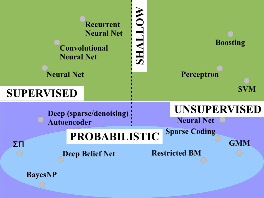
THE SPACE OF MACHINE LEARNING METHODS

21
PerceptronNeural Net
Boosting
SVM
GMMΣΠ
BayesNP
Convolutional Neural Net
Recurrent Neural Net
AutoencoderNeural Net
Sparse Coding
Restricted BMDeep Belief Net
Deep (sparse/denoising) Autoencoder

22
PerceptronNeural Net
Boosting
SVM
GMMΣΠ
BayesNP
Convolutional Neural Net
Recurrent Neural Net
AutoencoderNeural Net
Sparse Coding
Restricted BMDeep Belief Net
Deep (sparse/denoising) Autoencoder
SHA
LL
OW
DE
EP

23
PerceptronNeural Net
Boosting
SVM
GMMΣΠ
BayesNP
Convolutional Neural Net
Recurrent Neural Net
AutoencoderNeural Net
Sparse Coding
Restricted BMDeep Belief Net
Deep (sparse/denoising) Autoencoder
UNSUPERVISED
SUPERVISED
DE
EP
SHA
LL
OW
24
PerceptronNeural Net
Boosting
SVM
Convolutional Neural Net
Recurrent Neural Net
AutoencoderNeural Net
Deep (sparse/denoising) Autoencoder
UNSUPERVISED
SUPERVISED
DE
EP
SHA
LL
OW
ΣΠ
BayesNP
Deep Belief NetGMM
Sparse Coding
Restricted BM
PROBABILISTIC

25
Main types of deep architectures
Ranzato
Deep Learning is B I G
input input
input
feed
-f orw
ard
Feed
- bac
k
Bi-d
irect
ion a
l
Neural nets Conv Nets
Hierar. Sparse Coding Deconv Nets
Stacked Auto-encoders DBM
input
Rec
urre
nt Recurrent Neural nets Recursive Nets LISTA

26
Ranzato
Deep Learning is B I G
input input
input
feed
-f orw
ard
Feed
- bac
k
Bi-d
irect
ion a
l
Neural nets Conv Nets
Hierar. Sparse Coding Deconv Nets
Stacked Auto-encoders DBM
input
Rec
urre
nt Recurrent Neural nets Recursive Nets LISTA
Main types of deep architectures

27
Ranzato
Deep Learning is B I G Main types of learning protocols
Purely supervisedBackprop + SGDGood when there is lots of labeled data.
Layer-wise unsupervised + superv. linear classifierTrain each layer in sequence using regularized auto-encoders or RBMsHold fix the feature extractor, train linear classifier on featuresGood when labeled data is scarce but there is lots of unlabeled data.
Layer-wise unsupervised + supervised backpropTrain each layer in sequenceBackprop through the whole systemGood when learning problem is very difficult.

28
Ranzato
Deep Learning is B I G Main types of learning protocols
Purely supervisedBackprop + SGDGood when there is lots of labeled data.
Layer-wise unsupervised + superv. linear classifierTrain each layer in sequence using regularized auto-encoders or RBMsHold fix the feature extractor, train linear classifier on featuresGood when labeled data is scarce but there is lots of unlabeled data.
Layer-wise unsupervised + supervised backpropTrain each layer in sequenceBackprop through the whole systemGood when learning problem is very difficult.

29
Outline
Theory: Energy-Based ModelsEnergy functionLoss function
Examples:Supervised learning: neural netsSupervised learning: convnetsUnsupervised learning: sparse codingUnsupervised learning: gated MRF
Other examples Practical tricks
Ranzato

30
Energy:
LeCun et al. “Tutorial on Energy-based learning ...” Predicting Structure Data 2006Ranzato et al. “A unified energy-based framework for unsup. learning” AISTATS 2007
Energy-Based Models: Energy Function
E y ; E y ; x ,or
unsupervised supervised

31
Energy:
LeCun et al. “Tutorial on Energy-based learning ...” Predicting Structure Data 2006Ranzato et al. “A unified energy-based framework for unsup. learning” AISTATS 2007
Energy-Based Models: Energy Function
E y ; E y ; x ,or
unsupervised supervised
y can be discrete
continuous{

32
Energy:
LeCun et al. “Tutorial on Energy-based learning ...” Predicting Structure Data 2006Ranzato et al. “A unified energy-based framework for unsup. learning” AISTATS 2007
Energy-Based Models: Energy Function
E y ; E y ; x ,or
unsupervised supervised
y can be discrete
continuous{
We will refer to the unsupervised/continous case, but much of the following applies to
the other cases as well.

33
Energy should be lower for desired output
E
y
Energy-Based Models: Energy Function
Ranzato

34
Make energy lower at the desired output
E
yy∗
BEFORE TRAINING
Energy-Based Models: Energy Function
Ranzato

35
Make energy lower at the desired output
E
yy∗
AFTER TRAINING
Energy-Based Models: Energy Function
Ranzato

36
Examples of energy function:
PCA
Linear binary classifier
Neural net binary classifier
Energy-Based Models: Energy Function
E y=∥y−W W T y∥22
E y ; x =− y W T x
y∈{−1,1}
E y ; x =− y W 2T f x ;W 1

37
Energy-Based Models: Loss Function
Loss is a function of the energy
Minimizing the loss over the training set yields the desired energy landscape.
∗=min∑ p
L E y p ;
Examples of loss function:PCA
Logistic regression classifier
E y=∥y−W W T y∥22
E y ; x =− y W T x
L E y=E y
L E y ; x =log 1exp E y ; x

38
Energy-Based Models: Loss Function
Loss is a function of the energy
Minimizing the loss over the training set yields the desired energy landscape.
∗=min∑ p
L E y p ;
How to design loss good functions?
Ranzato

39
Energy-Based Models: Loss Function
Loss is a function of the energy
Minimizing the loss over the training set yields the desired energy landscape.
∗=min∑ p
L E y p ;
E
y
L=E y
How to design loss good functions?

40
Energy-Based Models: Loss Function
Loss is a function of the energy
Minimizing the loss over the training set yields the desired energy landscape.
∗=min∑ p
L E y p ;
E
y
L=E y
How to design loss good functions?

41
Energy-Based Models: Loss Function
Loss is a function of the energy
Minimizing the loss over the training set yields the desired energy landscape.
∗=min∑ p
L E y p ;
E
y
L=E y
BAD LOSS
How to design loss good functions?
Energy is degenerate:low everywhere!

42
Energy-Based Models: Loss Function
Loss is a function of the energy
Minimizing the loss over the training set yields the desired energy landscape.
∗=min∑ p
L E y p ;
How to design loss good functions?
L=E y log ∑yexp−E y
E
y

43
Energy-Based Models: Loss Function
Loss is a function of the energy
Minimizing the loss over the training set yields the desired energy landscape.
∗=min∑ p
L E y p ;
How to design loss good functions?
L=E y log ∑yexp−E y
E
y
GOOD LOSSbut potentially very expensive

44
Strategies to Shape E: #1 Pull down the correct answer and pull up everywhere else.
E
y
L=E y log ∑yexp−E y
PROS It produces calibrated probabilities.
CONS Expensive to compute when y is discrete and high dimensional. Generally intractable when y is continuous.
Negative Log-Likelihood
p y=e−E y
∑ue−E u

45
Strategies to Shape E: #2 Pull down the correct answer and pull up carefully chosen points.
L=max0,m−E y −E y , e.g. y=min y≠ y E y
E
yy
E.g.: Contrastive Divergence, Ratio Matching, Noise Contrastive Estimation, Minimum Probability Flow...
Hinton et al. “A fast learning algorithm for DBNs” Neural Comp. 2008
Gutmann et al. “Noise contrastive estimation of unnormalized...” JMLR 2012Hyvarinen “Some extensions of score matchine” Comp Stats 2007
Sohl-Dickstein et al. “Minimum probability flow learning” ICML 2011

46
Strategies to Shape E: #2 Pull down the correct answer and pull up carefully chosen points.
PROS Efficient.
CONS The criterion to pick where to pull up is tricky (overall in high dimensional spaces): trades-off computational and statistical efficiency.
L=max0,m−E y −E y , e.g. y=min y≠ y E y
E
yy

47
Strategies to Shape E: #3 Pull down the correct answer and increase local curvature.
E
y
Score Matching
L= ∂E y ∂ y
2
∂2 E y
∂ y2
Hyvarinen “Estimation of non-normalized statistical models using score matching” JMLR 2005

48
Strategies to Shape E: #3 Pull down the correct answer and increase local curvature.
E Score Matching
y
Hyvarinen “Estimation of non-normalized statistical models using score matching” JMLR 2005
L= ∂E y ∂ y
2
∂2 E y
∂ y2

49
Strategies to Shape E: #3 Pull down the correct answer and increase local curvature.
PROS Efficient in continuous but not too high dimensional spaces.
CONS Very complicated to compute and not practical in very high dimensional spaces. Not applicable in discrete spaces.
E Score Matching
y
L= ∂E y ∂ y
2
∂2 E y
∂ y2

50
Strategies to Shape E: #4 Pull down correct answer and have global constrain on the energy: only few minima exist
E
y
PCA, ICA, sparse coding,...
PROS Efficient in continuous, high dimensional spaces.
L=E y
Ranzato et al. “A unified energy-based framework for unsup. learning” AISTATS 2007
CONS Need to design good global constraints. Used in unsup. learning only.

51
Strategies to Shape E: #4
E
y
PCA, ICA, sparse coding,...
L=E y
Pull down correct answer and have global constrain on the energy: only few minima exist
PROS Efficient in continuous, high dimensional spaces.
CONS Need to design good global constraints. Used in unsup. learning only.
Ranzato et al. “A unified energy-based framework for unsup. learning” AISTATS 2007

52
Strategies to Shape E: #4 Pull down correct answer and have global constrain on the energy: only few minima exist
Typical methods (unsup. learning):Use compact internal representation (PCA)Have finite number of internal states (K-Means)Use sparse codes (ICA, sparse coding)
Ranzato

53
INPUT SPACE: FEATURE SPACE:
f x , h
g x , h
hx
Ranzato
training sampleinput data point which is not a training samplefeature (code)

54
Wh
f x , h
hxINPUT SPACE: FEATURE SPACE:
E.g. K-means: is 1-of-N.h
Since there are very few “codes” available and the energy (MSE) is minimized on the training set, the energy must be higher elsewhere.
Ranzato

55
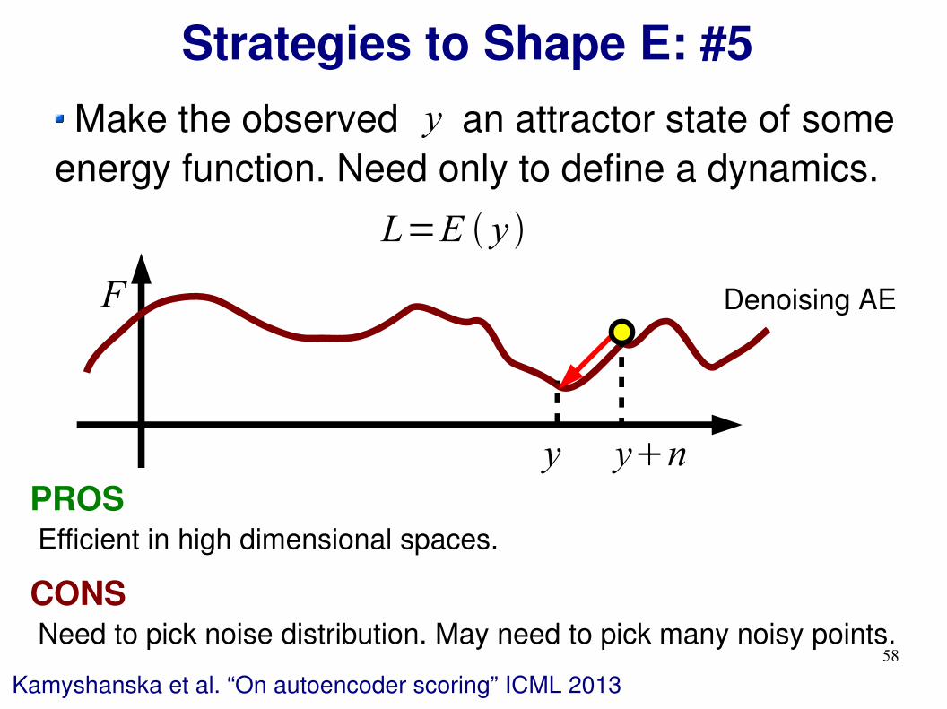
Strategies to Shape E: #5
F Denoising AE
L=E y
Make the observed an attractor state of some energy function. Need only to define a dynamics.
y
E.g.:
L=12∥y−y∥
2
y=W 2 W 1 yn , n∈N 0, I
y
Vincent et al. “Extracting and composing robust features with denoising autoencoders” ICML 2008
Training samples must be stable points (local minima)and attractors.

56
Make the observed an attractor state of some energy function. Need only to define a dynamics.
Strategies to Shape E: #5
Denoising AE
E.g.:yn
Training samples must be stable points (local minima)and attractors.
F
Kamyshanska et al. “On autoencoder scoring” ICML 2013
y
L=E y
y
y=W 2 W 1 yn , n∈N 0, I
L=12∥y−y∥
2
Ranzato

57
Make the observed an attractor state of some energy function. Need only to define a dynamics.
Strategies to Shape E: #5
Denoising AE
E.g.:
F
Training samples must be stable points (local minima)and attractors.
Kamyshanska et al. “On autoencoder scoring” ICML 2013
y
L=E y
y yn
y=W 2 W 1 yn , n∈N 0, I
L=12∥y−y∥
2
Ranzato
58
Make the observed an attractor state of some energy function. Need only to define a dynamics.
Strategies to Shape E: #5
PROS Efficient in high dimensional spaces.
CONS Need to pick noise distribution. May need to pick many noisy points.
Kamyshanska et al. “On autoencoder scoring” ICML 2013
Denoising AEF
y
L=E y
y yn

59
Loss: summary
Goal of loss: make energy lower for correct answer.
Different losses choose differently how to “pull-up”Pull-up all pointsPull up one or a few points onlyMake observations minima & increase curvatureAdd global constraints/penalties on internal statesDefine a dynamics with observations at the minima
Choice of loss depends on desired landscape, computational budget, domain of input (discrete/continouus), task, etc.
Ranzato

60
Final Notes on EBMs
EBMs apply to any predictor (shallow & deep).
EBMs subsume graphical models (e.g., use strategy #1 or #2 to “pull-up”).
EBM is general framework to design good loss functions.
Ranzato

61
Outline
Theory: Energy-Based ModelsEnergy functionLoss function
Examples:Supervised learning: neural netsSupervised learning: convnetsUnsupervised learning: sparse codingUnsupervised learning: gated MRF
Other examples Practical tricks
Ranzato

62
Perceptron
Neural Net
Boosting
SVM
GMM
ΣΠ
BayesNP
CNN
Recurrent Neural Net
AutoencoderNeural Net
Sparse Coding
Restricted BMDBN
Deep (sparse/denoising) Autoencoder
UNSUPERVISED
SUPERVISED
DE
EP
SHA
LL
OW
PROBABILISTIC
Loss: type #1

63
Neural Nets
NOTE: In practice, any (a.e. differentiable) non-linear transformation can be used.
h2h1xmax 0,W 1 x
h3max 0,W 2h1 W 3h2
Ranzato
64
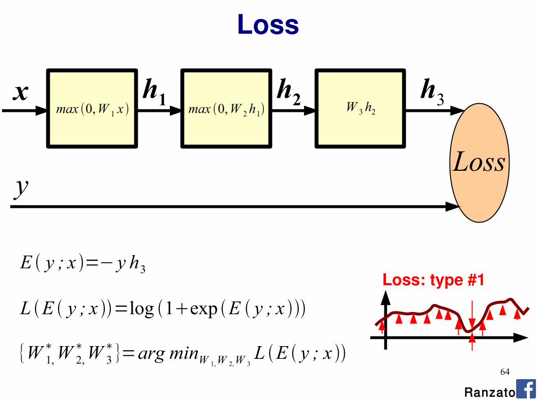
Loss
h2h1x h3
Lossy
max 0,W 1 x max 0,W 2h1 W 3h2
L E y ; x =log 1exp E y ; x
E y ; x =− y h3
{W 1,∗ W 2,
∗ W 3∗}=arg minW 1,W 2,W 3
L E y ; x
Loss: type #1
Ranzato

65
Loss
h2h1x h3
Lossy
max 0,W 1 x max 0,W 2h1 W 3h2
Q.: how to tune the parameters to decrease the loss?
If loss is (a.e.) differentiable we can compute gradients.
We can use chain-rule, a.k.a. back-propagation, to compute the gradients w.r.t. parameters at the lower layers.
Rumelhart et al. “Learning internal representations by back-propagating..” Nature 1986

66
Backward Propagation
h2h1x
Lossy
Given and assuming we can easily compute the Jacobian of each module, we have:
∂ L/∂h3
∂ L∂h2
=∂ L∂h3
∂h3∂h2
∂ L∂W 3
=∂ L∂h3
∂h3∂W 3
∂L∂h3
∂ L∂W 3
= h3− y h2T
max 0,W 1 x max 0,W 2h1 W 3h2
∂ L∂h2
= W 3T h3− y

67
Backward Propagation
h1x
Lossy
Given we can compute now:∂ L∂h2
∂ L∂h1
=∂ L∂h2
∂ h2∂h1
∂ L∂W 2
=∂ L∂h2
∂ h2∂W 2
∂L∂h3
∂ L∂h2 W 3h2max 0,W 2h1max 0,W 1 x
Ranzato

68
Backward Propagation
x
Lossy
Given we can compute now:∂ L∂h1
∂ L∂W 1
=∂ L∂h1
∂ h1∂W 1
∂L∂h3
∂ L∂h2
∂ L∂h1 W 3h2max 0,W 2h1max 0,W 1 x
Ranzato

69
Optimization
Stochastic Gradient Descent (on mini-batches):
−∂ L∂
,∈R
Stochastic Gradient Descent with Momentum:
0.9∂L∂
−
Ranzato

70
Toy Code (Matlab): Neural Net Trainer% F-PROPfor i = 1 : nr_layers - 1 [h{i} jac{i}] = nonlinearity(W{i} * h{i-1} + b{i});endh{nr_layers-1} = W{nr_layers-1} * h{nr_layers-2} + b{nr_layers-1};prediction = softmax(h{l-1});
% CROSS ENTROPY LOSSloss = - sum(sum(log(prediction) .* target)) / batch_size;
% B-PROPdh{l-1} = prediction - target;for i = nr_layers – 1 : -1 : 1 Wgrad{i} = dh{i} * h{i-1}'; bgrad{i} = sum(dh{i}, 2); dh{i-1} = (W{i}' * dh{i}) .* jac{i-1}; end
% UPDATEfor i = 1 : nr_layers - 1 W{i} = W{i} – (lr / batch_size) * Wgrad{i}; b{i} = b{i} – (lr / batch_size) * bgrad{i}; end
Ranzato

71
Perceptron
Neural Net
Boosting
SVM
GMM
ΣΠ
BayesNP
CNN
Recurrent Neural Net
AutoencoderNeural Net
Sparse Coding
Restricted BMDBN
Deep (sparse/denoising) Autoencoder
UNSUPERVISED
SUPERVISED
DE
EP
SHA
LL
OW
PROBABILISTIC
Loss: type #1

72
Example: 200x200 image 40K hidden units
~2B parameters!!!
- Spatial correlation is local- Better to put resources elsewhere!
FULLY CONNECTED NEURAL NET
Ranzato

73
LOCALLY CONNECTED NEURAL NET
Example: 200x200 image 40K hidden units Filter size: 10x10
4M parameters
Ranzato

74
STATIONARITY? Statistics are similar at different locations
Example: 200x200 image 40K hidden units Filter size: 10x10
4M parameters
LOCALLY CONNECTED NEURAL NET
Ranzato

75
CONVOLUTIONAL NET
Share the same parameters across different locations (assuming input is stationary):Convolutions with learned kernels
Ranzato

76
Learn multiple filters.
E.g.: 200x200 image 100 Filters Filter size: 10x10
10K parameters
NOTE: filter responses are non-linearly transformed:
CONVOLUTIONAL NET
h=max0, x∗wRanzato

77
KEY IDEAS
A standard neural net applied to images:- scales quadratically with the size of the input- does not leverage stationarity
Solution:- connect each hidden unit to a small patch of the input- share the weight across hidden units
This is called: convolutional layer.A network with convolutional layers is called convolutional network.
LeCun et al. “Gradient-based learning applied to document recognition” IEEE 1998

78
Let us assume filter is an “eye” detector.
Q.: how can we make the detection robust to the exact location of the eye?
POOLING
Ranzato

79
By “pooling” (e.g., taking max) filterresponses at different locations we gainrobustness to the exact spatial locationof features.
POOLING
Ranzato

80
LOCAL CONTRAST NORMALIZATION
h i1, x , y=hi , x , y−mi , N x , y
i , N x , y
Ranzato

81
LOCAL CONTRAST NORMALIZATION
h i1, x , y=hi , x , y−mi , N x , y
i , N x , y
We want the same response.
Ranzato

82
LOCAL CONTRAST NORMALIZATION
h i1, x , y=hi , x , y−mi , N x , y
i , N x , y
Performed also across features and in the higher layers.
Effects:– improves invariance– improves optimization– increases sparsity
Ranzato

83
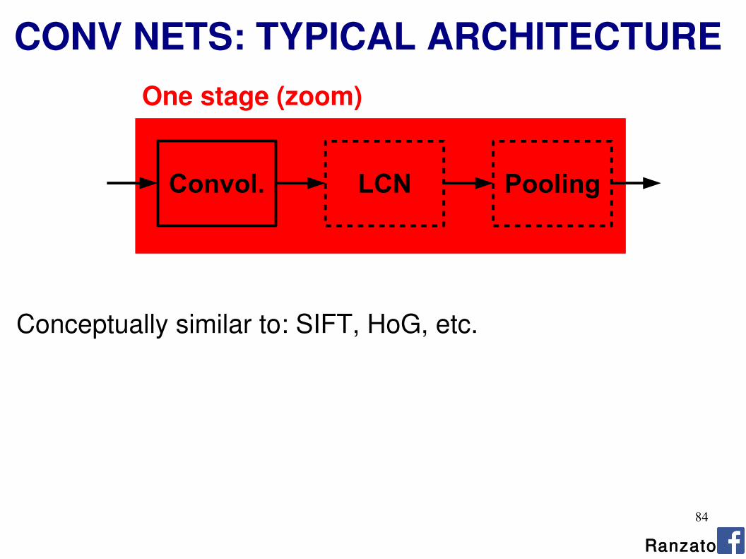
CONV NETS: TYPICAL ARCHITECTURE
Convol. LCN Pooling
One stage (zoom)
courtesy of K. Kavukcuoglu Ranzato
84
CONV NETS: TYPICAL ARCHITECTURE
Convol. LCN Pooling
One stage (zoom)
Conceptually similar to: SIFT, HoG, etc.
Ranzato

85
CONV NETS: TYPICAL ARCHITECTURE
Convol. LCN Pooling
One stage (zoom)
Fully Conn. Layers
Whole system
1st stage 2nd stage 3rd stage
Input Image
ClassLabels
Ranzato

86
CONV NETS: TYPICAL ARCHITECTURE
SIFT → K-Means → Pyramid Pooling → SVM
SIFT → Fisher Vect. → Pooling → SVM
Lazebnik et al. “...Spatial Pyramid Matching...” CVPR 2006
Sanchez et al. “Image classifcation with F.V.: Theory and practice” IJCV 2012
Conceptually similar to:
Ranzato
Fully Conn. Layers
Whole system
1st stage 2nd stage 3rd stage
Input Image
ClassLabels

87
CONV NETS: TRAINING
Algorithm:Given a small mini-batch- F-PROP- B-PROP- PARAMETER UPDATE
All layers are differentiable (a.e.). We can use standard back-propagation.
Ranzato

88
CONV NETS: EXAMPLES- OCR / House number & Traffic sign classification
Ciresan et al. “MCDNN for image classification” CVPR 2012Wan et al. “Regularization of neural networks using dropconnect” ICML 2013

89
CONV NETS: EXAMPLES- Texture classification
Sifre et al. “Rotation, scaling and deformation invariant scattering...” CVPR 2013

90
CONV NETS: EXAMPLES- Pedestrian detection
Sermanet et al. “Pedestrian detection with unsupervised multi-stage..” CVPR 2013

91
CONV NETS: EXAMPLES- Scene Parsing
Farabet et al. “Learning hierarchical features for scene labeling” PAMI 2013RanzatoPinheiro et al. “Recurrent CNN for scene parsing” arxiv 2013

92
CONV NETS: EXAMPLES- Segmentation 3D volumetric images
Ciresan et al. “DNN segment neuronal membranes...” NIPS 2012Turaga et al. “Maximin learning of image segmentation” NIPS 2009 Ranzato

93
CONV NETS: EXAMPLES- Action recognition from videos
Taylor et al. “Convolutional learning of spatio-temporal features” ECCV 2010

94
CONV NETS: EXAMPLES- Robotics
Sermanet et al. “Mapping and planning ...with long range perception” IROS 2008

95
CONV NETS: EXAMPLES- Denoising
Burger et al. “Can plain NNs compete with BM3D?” CVPR 2012
original noised denoised
Ranzato

96
CONV NETS: EXAMPLES- Dimensionality reduction / learning embeddings
Hadsell et al. “Dimensionality reduction by learning an invariant mapping” CVPR 2006

97
CONV NETS: EXAMPLES- Object detection
Sermanet et al. “OverFeat: Integrated recognition, localization, ...” arxiv 2013
Szegedy et al. “DNN for object detection” NIPS 2013 RanzatoGirshick et al. “Rich feature hierarchies for accurate object detection...” arxiv 2013

98
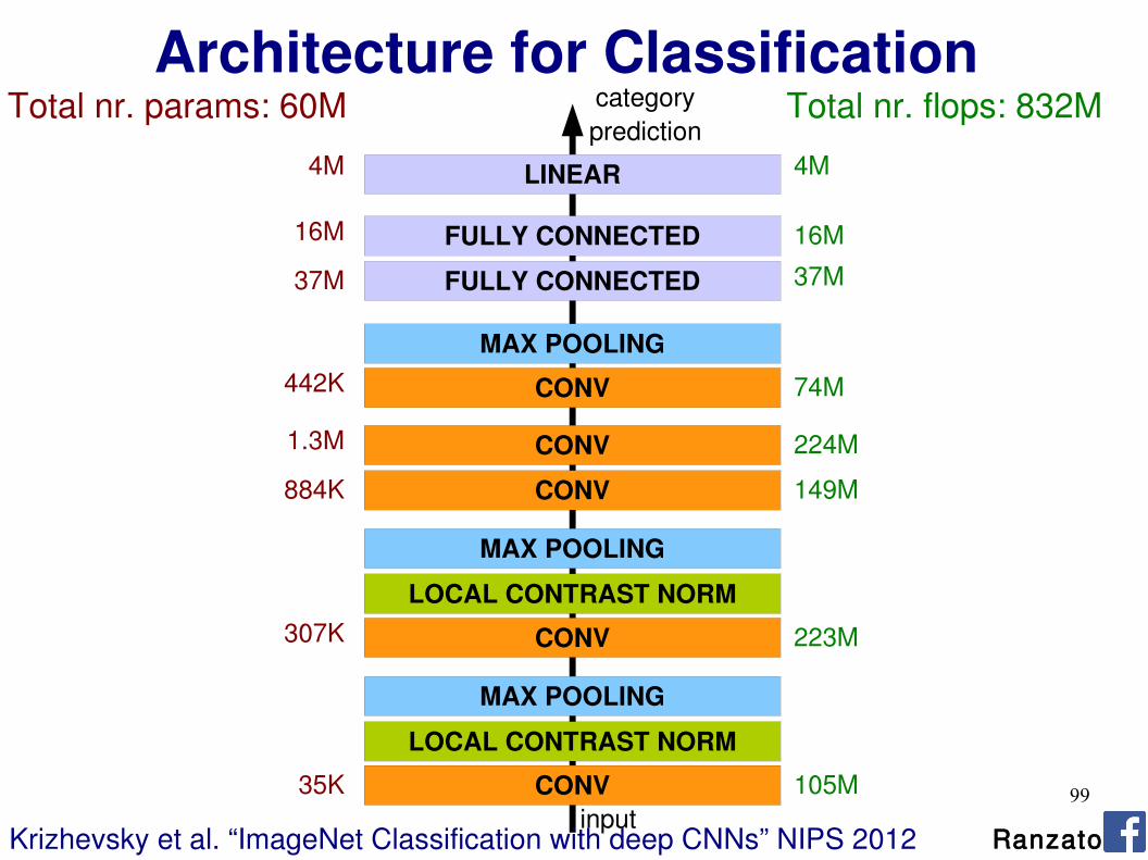
Architecture for Classification
CONV
LOCAL CONTRAST NORM
MAX POOLING
FULLY CONNECTED
LINEAR
CONV
LOCAL CONTRAST NORM
MAX POOLING
CONV
CONV
CONV
MAX POOLING
FULLY CONNECTED
Krizhevsky et al. “ImageNet Classification with deep CNNs” NIPS 2012
category prediction
input Ranzato
99CONV
LOCAL CONTRAST NORM
MAX POOLING
FULLY CONNECTED
LINEAR
CONV
LOCAL CONTRAST NORM
MAX POOLING
CONV
CONV
CONV
MAX POOLING
FULLY CONNECTED
Total nr. params: 60M
4M
16M
37M
442K
1.3M
884K
307K
35K
Total nr. flops: 832M
4M
16M37M
74M
224M
149M
223M
105M
Krizhevsky et al. “ImageNet Classification with deep CNNs” NIPS 2012
category prediction
input Ranzato
Architecture for Classification

100
Optimization
SGD with momentum:
Learning rate = 0.01
Momentum = 0.9
Improving generalization by:
Weight sharing (convolution)
Input distortions
Dropout = 0.5
Weight decay = 0.0005
Ranzato
101
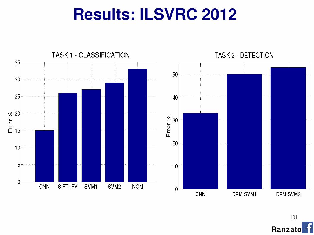
Results: ILSVRC 2012
Ranzato

102
Results
First layer learned filters (processing raw pixel values).
Krizhevsky et al. “ImageNet Classification with deep CNNs” NIPS 2012 Ranzato

103
104
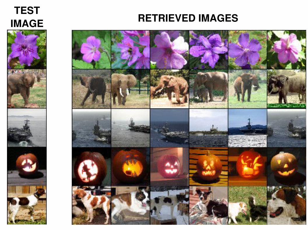
TEST IMAGE RETRIEVED IMAGES

105
http://horatio.cs.nyu.edu/
Demo of classifier by Matt Zeiler & Rob Fergus:

106
http://decafberkeleyvision.org/
Demo of classifier by Yangqing Jia & Trevor Darrell:
DeCAF arXiv 1310.1531 2013

107
1 10 1001
10
100
nr. training samples
% e
rror
DeCAF (1M images)
Donahue, Jia et al. DeCAF arXiv 1310.1531 2013Excerpt from Perona Visual Recognition 2007
Ranzato

108
Outline
Theory: Energy-Based ModelsEnergy functionLoss function
Examples:Supervised learning: neural netsSupervised learning: convnetsUnsupervised learning: sparse codingUnsupervised learning: gated MRF
Other examples Practical tricks
Ranzato

109
Perceptron
Neural Net
Boosting
SVM
GMM
ΣΠ
BayesNP
CNN
Recurrent Neural Net
AutoencoderNeural Net
Sparse Coding
Restricted BMDBN
Deep (sparse/denoising) Autoencoder
UNSUPERVISED
SUPERVISED
DE
EP
SHA
LL
OW
PROBABILISTIC Loss: type #4

110
Energy & latent variables
Energy may have latent variables.
Two major approaches:Marginalization (intractable if space is large)
Minimization
E y =minh E y ,h
E y =log∑hexp −E y ,h
Ranzato

111
Sparse Coding
L= E x ;W
E x ,h ;W =12∥x−W h∥2
2∥h∥1
E x ;W =minhE x ,h ;W Loss type #4: energy loss with (sparsity) constraints.
Ranzato et al. NIPS 2006Olshausen & Field, Nature 1996

112
Inference
Prediction of latent variables
h∗=arg minhE x ,h ; W
Inference is an iterative process.
E x ,h ;W =12∥x−W h∥2
2∥h∥1
Ranzato

113
Inference
Prediction of latent variables
h∗=arg minhE x ,h ; W
Inference is an iterative process.
E x ,h ;W =12∥x−W h∥2
2∥h∥1
Q.: Is it possible to make inference more efficient?A.: Yes, by training another module to directly predict
Kavukcuoglu et al. “Predictive Sparse Decomposition” ArXiv 2008
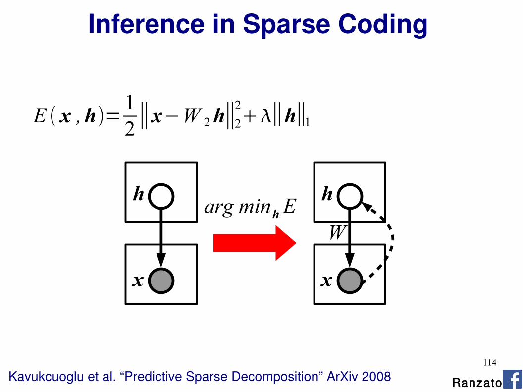
114
Inference in Sparse Coding
E x ,h=12∥x−W 2h∥2
2∥h∥1
Kavukcuoglu et al. “Predictive Sparse Decomposition” ArXiv 2008
x
h
x
h
Warg minhE
Ranzato
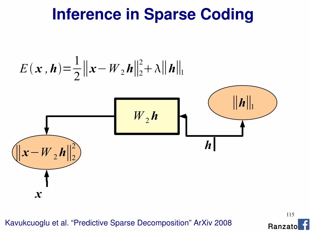
115
E x ,h=12∥x−W 2h∥2
2∥h∥1
Kavukcuoglu et al. “Predictive Sparse Decomposition” ArXiv 2008
W 2h
∥x−W 2h∥22
∥h∥1
h
x
Inference in Sparse Coding
Ranzato

116
Learning To Perform Fast Inference
E x ,h=12∥x−W 2h∥2
2∥h∥1
12∥h−g x ;W 1∥2
2
Kavukcuoglu et al. “Predictive Sparse Decomposition” ArXiv 2008
g x ;W 1
∥h−g x ;W 1∥22
h
x
Ranzato

117
Predictive Sparse Decomposition
E x ,h=12∥x−W 2h∥2
2∥h∥1
12∥h−g x ;W 1∥2
2
Kavukcuoglu et al. “Predictive Sparse Decomposition” ArXiv 2008
g x ;W 1
W 2h
∥x−W 2h∥22
∥h−g x ;W 1∥22
∥h∥1
h
x
Ranzato

118
Sparse Auto-Encoders
Example: Predictive Sparse Decomposition
E x ,h=12∥x−W 2h∥2
2∥h∥1
12∥h−g x ;W 1∥2
2
Kavukcuoglu et al. “Predictive Sparse Decomposition” ArXiv 2008
TRAINING:
For every sample: Initialize (E) Infer optimal latent variables: (M) Update parameters
h=g x ;W 1h∗=minhE x ,h ;W
W 1 , W 2
Inference at test time (fast):h∗≈g x ;W 1
Ranzato

119
E x ,h=12∥x−W 2h∥2
2∥h∥1
12∥h−g x ;W 1∥2
2
Kavukcuoglu et al. “Predictive Sparse Decomposition” ArXiv 2008
x
h
W x h
alternative graphical representations
Predictive Sparse Decomposition
Ranzato

120
Gregor et al. “Learning fast approximations of sparse coding” ICML 2010
LISTA
W 1
W 2
∥x−W 2h∥22
∥h−g x ;W 1∥22
∥h∥1
h
x
++W 3 W 3 W 3
Ranzato

121
KEY IDEAS
Inference can require expensive optimization
We may approximate exact inference well by using a non-linear function (learn optimal approximation to perform fast inference)
The original model and the fast predictor can be trained jointly
Kavukcuoglu et al. “Predictive Sparse Decomposition” ArXiv 2008
Rolfe et al. “Discriminative Recurrent Sparse Autoencoders” ICLR 2013Szlam et al. “Fast approximations to structured sparse coding...” ECCV 2012Gregor et al. “Structured sparse coding via lateral inhibition” NIPS 2011Kavukcuoglu et al. “Learning convolutonal feature hierarchies..” NIPS 2010
Ranzato

122
Outline
Theory: Energy-Based ModelsEnergy functionLoss function
Examples:Supervised learning: neural netsSupervised learning: convnetsUnsupervised learning: sparse codingUnsupervised learning: gated MRF
Other examples Practical tricks
Ranzato

123
Perceptron
Neural Net
Boosting
SVM
GMM
ΣΠ
BayesNP
CNN
Recurrent Neural Net
AutoencoderNeural Net
Sparse Coding
Restricted BMDBN
Deep (sparse/denoising) Autoencoder
UNSUPERVISED
SUPERVISED
DE
EP
SHA
LL
OW
PROBABILISTIC
Loss: type #2

124
Probabilistic Models of Natural Images
INPUT SPACE LATENT SPACE
Training sample Latent vector
p x∣h=N meanh , D
- examples: PPCA, Factor Analysis, ICA, Gaussian RBM
p x∣h
Ranzato

125
Probabilistic Models of Natural Images
input image
model does not represent well dependecies, only mean intensity
ph∣x p x∣h
generated imagelatent variables
p x∣h=N meanh , D
- examples: PPCA, Factor Analysis, ICA, Gaussian RBM
Ranzato

126
Probabilistic Models of Natural Images
Training sample Latent vector
p x∣h=N 0,Covariance h
- examples: PoT, cRBM
p x∣h
Welling et al. NIPS 2003, Ranzato et al. AISTATS 10
INPUT SPACE LATENT SPACE
Ranzato

127
Probabilistic Models of Natural Images
Welling et al. NIPS 2003, Ranzato et al. AISTATS 10
model does not represent well mean intensity, only dependencies
Andy Warhol 1960
input image
ph∣x p x∣h
generated imagelatent variables
p x∣h=N 0,Covariance h
- examples: PoT, cRBM

128
Probabilistic Models of Natural Images
Training sample Latent vector
p x∣h=N mean h ,Covariance h
- this is what we propose: mcRBM, mPoT
Ranzato et al. CVPR 10, Ranzato et al. NIPS 2010, Ranzato et al. CVPR 11
p x∣h
INPUT SPACE LATENT SPACE
Ranzato

129
Probabilistic Models of Natural Images
Training sample Latent vector
Ranzato et al. CVPR 10, Ranzato et al. NIPS 2010, Ranzato et al. CVPR 11
p x∣h
p x∣h=N mean h ,Covariance h
- this is what we propose: mcRBM, mPoT
INPUT SPACE LATENT SPACE
Ranzato

130
PoT PPCA
Our model
N(0,Σ) N(m,I)
N(m,Σ)Ranzato

131
Deep Gated MRFLayer 1:
E x , hc
, hm=12
x ' −1
x
pair-wise MRFx p xq
Ranzato et al. “Modeling natural images with gated MRFs” PAMI 2013
p x , hc , hm e−E x , hc ,h m
Ranzato

132
Deep Gated MRFLayer 1:
E x , hc
, hm=12
x ' C C ' x
pair-wise MRFx p xq
F
Ranzato et al. “Modeling natural images with gated MRFs” PAMI 2013 Ranzato

133
Deep Gated MRFLayer 1:
E x , hc
, hm=12
x ' C [diag hc]C ' x
gated MRF
x p xq
hkc
CCF
F
Ranzato et al. “Modeling natural images with gated MRFs” PAMI 2013 Ranzato

134
Deep Gated MRF
Ranzato et al. “Modeling natural images with gated MRFs” PAMI 2013
Layer 1:
E x , hc
, hm=12
x ' C [diag hc]C ' x
12
x ' x− x ' W hm
x p xq
h jm
W
CCF
M
hkc
N
gated MRF
p x ∫hc∫hm e−E x ,hc , hm

135
Deep Gated MRF
Ranzato et al. “Modeling natural images with gated MRFs” PAMI 2013
Layer 1:
E x , hc
, hm=12
x ' C [diag hc]C ' x
12
x ' x− x ' W hm
Inference of latent variables: just a forward pass
Training:requires approximations
(here we used HMC with PCD)
p x ∫hc∫hm e−E x ,hc , hm
Loss: type #2

136
Deep Gated MRF
Ranzato et al. “Modeling natural images with gated MRFs” PAMI 2013
Layer 1:
E x , hc
, hm=12
x ' C [diag hc]C ' x
12
x ' x− x ' W hm
Inference of latent variables: just a forward pass
Training:requires approximations
(here we used HMC with PCD)
p x ∫hc∫hm e−E x ,hc , hm
Loss: type #2

137
Deep Gated MRF
Ranzato et al. “Modeling natural images with gated MRFs” PAMI 2013
Layer 1:
E x , hc
, hm=12
x ' C [diag hc]C ' x
12
x ' x− x ' W hm
Inference of latent variables: just a forward pass
Training:requires approximations
(here we used HMC with PCD)
p x ∫hc∫hm e−E x ,hc , hm
Loss: type #2
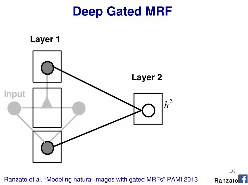
138
Deep Gated MRF
Ranzato et al. “Modeling natural images with gated MRFs” PAMI 2013
Layer 1
Layer 2
inputh2
Ranzato

139
Deep Gated MRF
Ranzato et al. “Modeling natural images with gated MRFs” PAMI 2013
Layer 1
h2
Layer 2
inputh3
Layer 3
Ranzato

140
Gaussian model marginal wavelet
from Simoncelli 2005
Pair-wise MRF FoE
from Schmidt, Gao, Roth CVPR 2010
Sampling High-Resolution Images

141
Gaussian model marginal wavelet
from Simoncelli 2005
Pair-wise MRF FoE
from Schmidt, Gao, Roth CVPR 2010
Sampling High-Resolution Images
gMRF: 1 layer
Ranzato et al. PAMI 2013

142
Gaussian model marginal wavelet
from Simoncelli 2005
Pair-wise MRF FoE
from Schmidt, Gao, Roth CVPR 2010
Sampling High-Resolution Images
Ranzato et al. PAMI 2013
gMRF: 1 layer

143
Gaussian model marginal wavelet
from Simoncelli 2005
Pair-wise MRF FoE
from Schmidt, Gao, Roth CVPR 2010
Sampling High-Resolution Images
Ranzato et al. PAMI 2013
gMRF: 1 layer

144
Gaussian model marginal wavelet
from Simoncelli 2005
Pair-wise MRF FoE
from Schmidt, Gao, Roth CVPR 2010
Sampling High-Resolution Images
Ranzato et al. PAMI 2013
gMRF: 3 layer
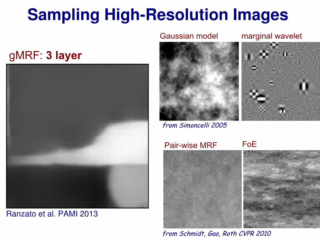
145
Gaussian model marginal wavelet
from Simoncelli 2005
Pair-wise MRF FoE
from Schmidt, Gao, Roth CVPR 2010
Sampling High-Resolution Images
Ranzato et al. PAMI 2013
gMRF: 3 layer

146
Gaussian model marginal wavelet
from Simoncelli 2005
Pair-wise MRF FoE
from Schmidt, Gao, Roth CVPR 2010
Sampling High-Resolution Images
Ranzato et al. PAMI 2013
gMRF: 3 layer

147
Gaussian model marginal wavelet
from Simoncelli 2005
Pair-wise MRF FoE
from Schmidt, Gao, Roth CVPR 2010
Sampling High-Resolution Images
Ranzato et al. PAMI 2013
gMRF: 3 layer

148
Sampling After Training on Face Images
Original Input 1st layer 2nd layer 3rd layer 4th layer 10 times
unconstrained samples
conditional (on the left part of the face) samples
Ranzato et al. PAMI 2013 Ranzato

149
Expression Recognition Under Occlusion
Ranzato et al. PAMI 2013 Ranzato

150
Tang et al. Robust BM for decognition and denoising CVPR 2012 Ranzato

151
Pros Cons Feature extraction is fast Unprecedented generation
quality Advances models of natural
images Trains without labeled data
Training is inefficientSlowTricky
Sampling scales badly with dimensionality What's the use case of
generative models?
Conclusion If generation is not required, other feature learning methods are
more efficient (e.g., sparse auto-encoders). What's the use case of generative models? Given enough labeled data, unsup. learning methods have not produced more useful features.

152
Outline
Theory: Energy-Based ModelsEnergy functionLoss function
Examples:Supervised learning: neural netsSupervised learning: convnetsUnsupervised learning: sparse codingUnsupervised learning: gated MRF
Other examples Practical tricks
Ranzato

153
RNNs
http://www.cs.toronto.edu/~graves/handwriting.html

154
Structured Prediction
LeCun et al. “Gradient-based learning applied to document recognition” IEEE 1998

155
Multi-Modal Learning
P A N D A
Frome et al. “DeVISE: A deep visual semantic embedding model” NIPS 2013Socher et al. Zero-shot learning though cross modal transfer” NIPS 2013

156
Multi-Modal Learning
Ngiam et al. “Multimodal deep learningl” ICML 2011Srivastava et al. “Multi-modal learning with DBM” ICML 2012 Ranzato

157
Outline
Theory: Energy-Based ModelsEnergy functionLoss function
Examples:Supervised learning: neural netsSupervised learning: convnetsUnsupervised learning: sparse codingUnsupervised learning: gated MRF
Other examples Practical tricks for CNNs
Ranzato

158
CHOOSING THE ARCHITECTURE
Task dependent
Cross-validation
[Convolution → LCN → pooling]* + fully connected layer
The more data: the more layers and the more kernelsLook at the number of parameters at each layerLook at the number of flops at each layer
Computational cost
Be creative :)Ranzato

159
HOW TO OPTIMIZE
SGD (with momentum) usually works very well
Pick learning rate by running on a subset of the dataBottou “Stochastic Gradient Tricks” Neural Networks 2012Start with large learning rate and divide by 2 until loss does not divergeDecay learning rate by a factor of ~1000 or more by the end of training
Use non-linearity
Initialize parameters so that each feature across layers has similar variance. Avoid units in saturation.
Ranzato

160
HOW TO IMPROVE GENERALIZATION
Weight sharing (greatly reduce the number of parameters)
Data augmentation (e.g., jittering, noise injection, etc.)
Dropout Hinton et al. “Improving Nns by preventing co-adaptation of feature detectors” arxiv 2012
Weight decay (L2, L1)
Sparsity in the hidden units
Multi-task (unsupervised learning)
Ranzato

161
ConvNets: till 2012
Loss
parameter
Common wisdom: training does not work because we “get stuck in local minima”
162
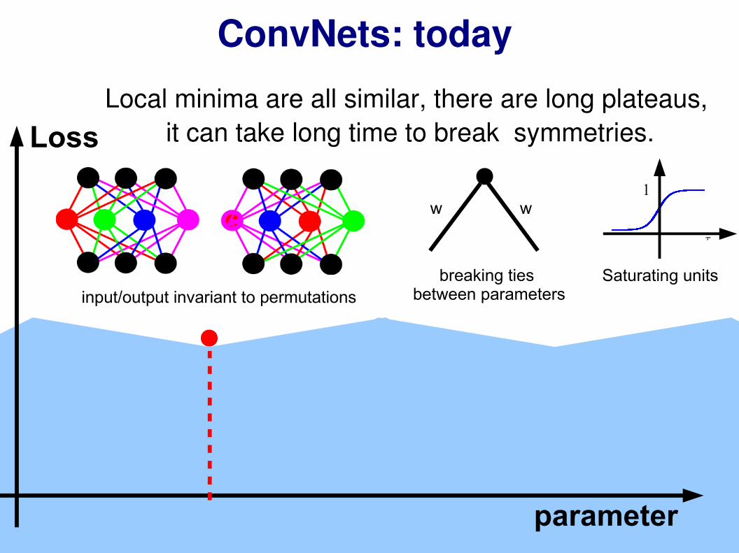
ConvNets: today
Loss
parameter
Local minima are all similar, there are long plateaus, it can take long time to break symmetries.
w w
input/output invariant to permutationsbreaking ties
between parameters
W T X
1
Saturating units

163
Like walking on a ridge between valleys
Neural Net Optimization is...

164
ConvNets: today
Loss
parameter
Local minima are all similar, there are long plateaus, it can take long to break symmetries.
Optimization is not the real problem when:– dataset is large– unit do not saturate too much– normalization layer

165
ConvNets: today
Loss
parameter
Today's belief is that the challenge is about:– generalization How many training samples to fit 1B parameters? How many parameters/samples to model spaces with 1M dim.?
– scalability

166
OTHER THINGS GOOD TO KNOW
Check gradients numerically by finite differences
Visualize features (feature maps need to be uncorrelated) and have high variance.
sam
p les
hidden unitGood training: hidden units are sparse across samples and across features. Ranzato

167
OTHER THINGS GOOD TO KNOW
Check gradients numerically by finite differences
Visualize features (feature maps need to be uncorrelated) and have high variance.
sam
p les
hidden unitBad training: many hidden units ignore the input and/or exhibit strong correlations. Ranzato
168
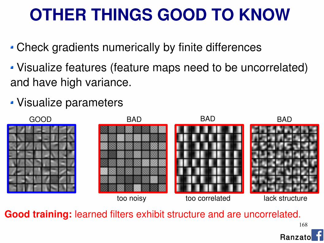
OTHER THINGS GOOD TO KNOW
Check gradients numerically by finite differences
Visualize features (feature maps need to be uncorrelated) and have high variance.
Visualize parameters
Good training: learned filters exhibit structure and are uncorrelated.
GOOD BADBAD BAD
too noisy too correlated lack structure
Ranzato

169
OTHER THINGS GOOD TO KNOW
Check gradients numerically by finite differences
Visualize features (feature maps need to be uncorrelated) and have high variance.
Visualize parameters
Measure error on both training and validation set.
Test on a small subset of the data and check the error → 0.
Ranzato

170
WHAT IF IT DOES NOT WORK?
Training diverges:Learning rate may be too large → decrease learning rateBPROP is buggy → numerical gradient checking
Parameters collapse / loss is minimized but accuracy is low Check loss function:
Is it appropriate for the task you want to solve?Does it have degenerate solutions? Check “pull-up” term.
Network is underperformingCompute flops and nr. params. → if too small, make net largerVisualize hidden units/params → fix optmization
Network is too slowCompute flops and nr. params. → GPU,distrib. framework, make net smaller
Ranzato

171
SUMMARY Deep Learning = Learning Hierarchical representations. Leverage compositionality to gain efficiency.
Unsupervised learning: active research topic.
Supervised learning: most successful set up today.
OptimizationDon't we get stuck in local minima? No, they are all the same!In large scale applications, local minima are even less of an issue.
ScalingGPUsDistributed framework (Google)Better optimization techniques
Generalization on small datasets (curse of dimensionality):Input distortions weight decay dropout Ranzato

172
THANK YOU!
Ranzato
NOTE: IJCV Special Issue on Deep Learning. Deadline: 9 Feb. 2014.

173
SOFTWARETorch7: learning library that supports neural net traininghttp://www.torch.chhttp://code.cogbits.com/wiki/doku.php (tutorial with demos by C. Farabet)
Python-based learning library (U. Montreal)
- http://deeplearning.net/software/theano/ (does automatic differentiation)
Caffe (Yangqing Jia)
– http://caffe.berkeleyvision.org
Efficient CUDA kernels for ConvNets (Krizhevsky)
– code.google.com/p/cuda-convnet
Ranzato

174
REFERENCESConvolutional Nets– LeCun, Bottou, Bengio and Haffner: Gradient-Based Learning Applied to Document Recognition, Proceedings of the IEEE, 86(11):2278-2324, November 1998
- Krizhevsky, Sutskever, Hinton “ImageNet Classification with deep convolutional neural networks” NIPS 2012
– Jarrett, Kavukcuoglu, Ranzato, LeCun: What is the Best Multi-Stage Architecture for Object Recognition?, Proc. International Conference on Computer Vision (ICCV'09), IEEE, 2009
- Kavukcuoglu, Sermanet, Boureau, Gregor, Mathieu, LeCun: Learning Convolutional Feature Hierachies for Visual Recognition, Advances in Neural Information Processing Systems (NIPS 2010), 23, 2010
– see yann.lecun.com/exdb/publis for references on many different kinds of convnets.
– see http://www.cmap.polytechnique.fr/scattering/ for scattering networks (similar to convnets but with less learning and stronger mathematical foundations)
– see http://www.idsia.ch/~juergen/ for other references to ConvNets and LSTMs.Ranzato

175
REFERENCESApplications of Convolutional Nets
– Farabet, Couprie, Najman, LeCun. Scene Parsing with Multiscale Feature Learning, Purity Trees, and Optimal Covers”, ICML 2012
– Pierre Sermanet, Koray Kavukcuoglu, Soumith Chintala and Yann LeCun: Pedestrian Detection with Unsupervised Multi-Stage Feature Learning, CVPR 2013
- D. Ciresan, A. Giusti, L. Gambardella, J. Schmidhuber. Deep Neural Networks Segment Neuronal Membranes in Electron Microscopy Images. NIPS 2012
- Raia Hadsell, Pierre Sermanet, Marco Scoffier, Ayse Erkan, Koray Kavackuoglu, Urs Muller and Yann LeCun. Learning Long-Range Vision for Autonomous Off-Road Driving, Journal of Field Robotics, 26(2):120-144, 2009
– Burger, Schuler, Harmeling. Image Denoisng: Can Plain Neural Networks Compete with BM3D?, CVPR 2012
– Hadsell, Chopra, LeCun. Dimensionality reduction by learning an invariant mapping, CVPR 2006
– Bergstra et al. Making a science of model search: hyperparameter optimization in hundred of dimensions for vision architectures, ICML 2013 Ranzato

176
REFERENCESDeep Learning in general
– deep learning tutorial slides at ICML 2013
– Yoshua Bengio, Learning Deep Architectures for AI, Foundations and Trends in Machine Learning, 2(1), pp.1-127, 2009.
– LeCun, Chopra, Hadsell, Ranzato, Huang: A Tutorial on Energy-Based Learning, in Bakir, G. and Hofman, T. and Schölkopf, B. and Smola, A. and Taskar, B. (Eds), Predicting Structured Data, MIT Press, 2006
Ranzato

177
THANK YOUAckknowledgements to Yann LeCun. Many slides from ICML 2013 and CVPR 2013 tutorial on deep learning.
IJCV SPECIAL ISSUE ON DEEP LEARNING: 9 Febrruary 2014.
Ranzato
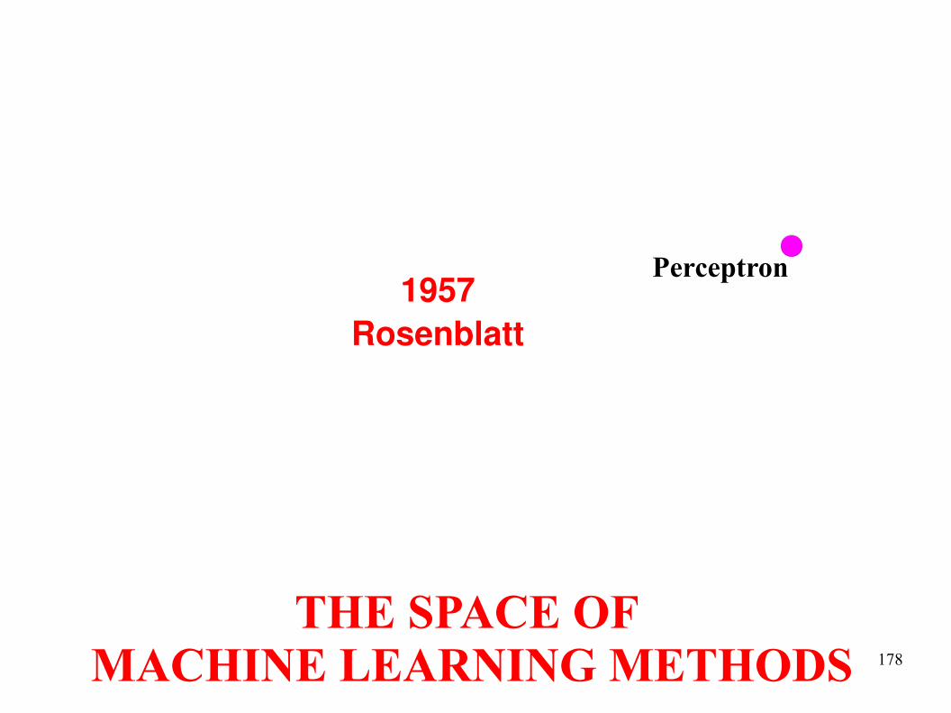
178
Perceptron1957
Rosenblatt
THE SPACE OF MACHINE LEARNING METHODS

179
PerceptronNeural Net
AutoencoderNeural Net
80s back-propagation &
compute power
Ranzato

180
PerceptronNeural Net
AutoencoderNeural Net
90s LeCun's CNNs
Convolutional Neural Net
Recurrent Neural Net
Sparse Coding
GMM
Ranzato

181
Perceptron
AutoencoderNeural Net
Convolutional Neural Net
Recurrent Neural Net
Sparse Coding
SVM
Boosting
GMMRestricted BM
Neural Net
00s SVMs
Ranzato

182
Perceptron
Boosting
SVM
GMM
BayesNP
Recurrent Neural Net
AutoencoderNeural Net
Sparse Coding
Restricted BM
Neural Net
Convolutional Neural Net
Deep Belief Net
2006 Hinton's DBN
Ranzato

183
GMM
BayesNP
Sparse Coding
Restricted BM
Neural Net
Deep Belief Net
Recurrent Neural Net
Boosting
Perceptron
AutoencoderNeural Net
Convolutional Neural Net
SVM
Deep (sparse/denoising) Autoencoder
ΣΠ
2009 ASR (data + GPU)
Ranzato
184
GMM
BayesNP
Sparse Coding
Restricted BM
Neural Net
Deep Belief Net
Recurrent Neural Net
Boosting
Perceptron
AutoencoderNeural Net
Convolutional Neural Net
SVM
Deep (sparse/denoising) Autoencoder
ΣΠ
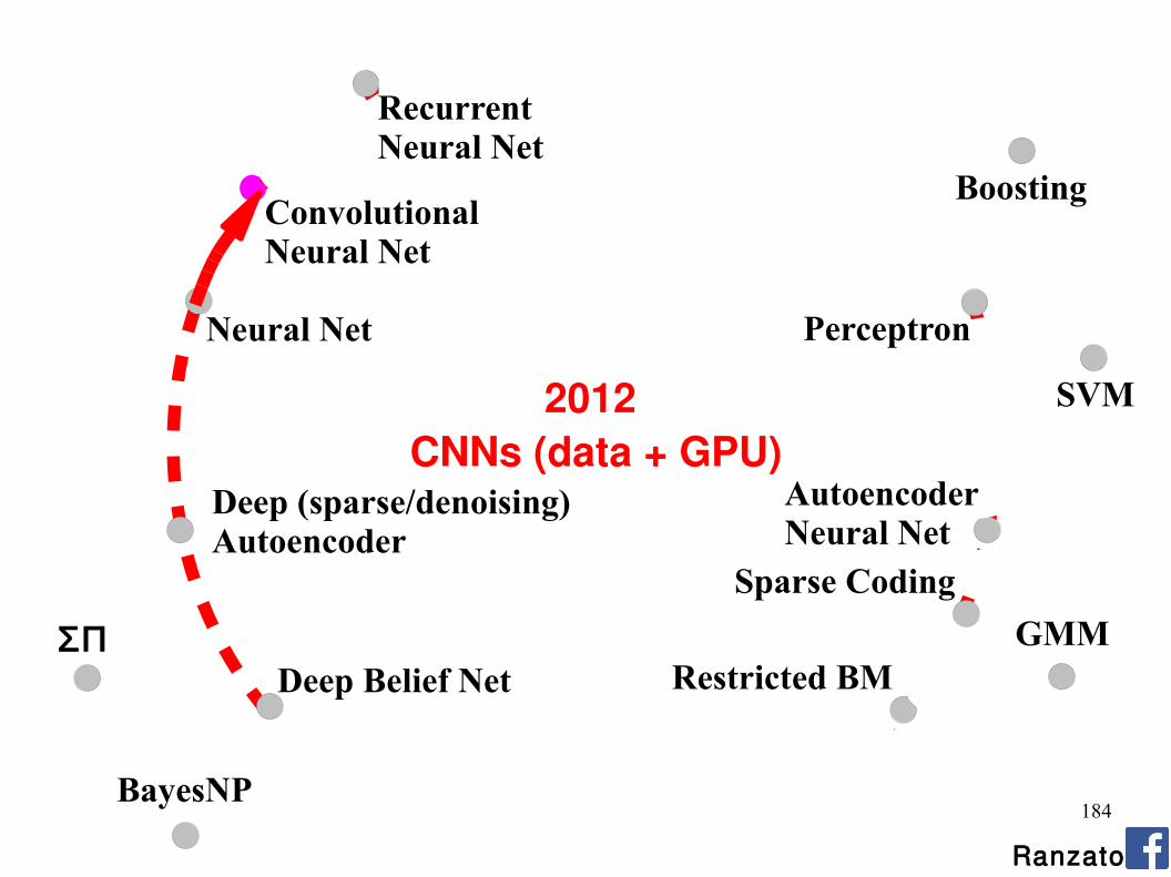
2012 CNNs (data + GPU)
Ranzato

185
PerceptronNeural Net
Boosting
SVM
GMMΣΠ
BayesNP
Convolutional Neural Net
Recurrent Neural Net
AutoencoderNeural Net
Sparse Coding
Restricted BMDeep Belief Net
Deep (sparse/denoising) Autoencoder
Ranzato

186
TIM
E
Convolutional Neural Net 2012
Convolutional Neural Net 1998
Convolutional Neural Net 1988
Q.: Did we make any prgress since then?
A.: The main reason for the breakthrough is: data and GPU, but we have also made networks deeper and more non-linear.
Ranzato

187
- 1980 Fukushima: designed network with same basic structure but did not train by backpropagation.
- late 80s LeCun: figured out backpropagation for CNN, popularized and deployed CNN for OCR applications and others.
- 1999 Poggio: same basic structure but learning is restricted to top layer (k-means at second stage)
- 2006 LeCun: unsupervised feature learning
- 2008 DiCarlo: large scale experiments, normalization layer
- 2009 LeCun: harsher non-linearities, normalization layer, learning unsupervised and supervised.
- 2011 Mallat: provides a theory behind the architecture
- 2012 Hinton: use bigger & deeper nets, GPUs, more data
LeCun et al. “Gradient-based learning applied to document recognition” IEEE 1998
ConvNets: History

188
data
flops/s
capacity
T IME
ConvNets: Why so successful now?
T IM
E
As time goes by, we get more data and more flops/s. The capacity of ML models
should grow accordingly.
1K 1M 1B
1M
100M
10T
Ranzato

189
data
capacity
T IME
ConvNets: Why so successful now?
CNN were in many ways premature, we did not have enough data and flops/s to train them.
They would overfit and be too slow to tran
(apparent local minima).
flops/s
1B
NOTE: methods have to be easily scalable!
Ranzato
![Optimization & Deep Learning 2017. 4. 19. · Z. Y LeCun Dynamic Factor Graphs Target Prop for Recurrent Nets Deep Learning for Time-Series Prediction – [Mirowski & LeCun ECML 09]](https://img.pdfslide.us/doc/110x75/6120d8d60885e46873566971/optimization-deep-learning-2017-4-19-z-y-lecun-dynamic-factor-graphs.jpg)


![arXiv:submit/2340273 [cs.CV] 24 Jul 2018cocosci.princeton.edu/papers/deep-sim-arxiv.pdf · understanding (LeCun, Bengio, & Hinton, 2015), among other breakthroughs in natural language](https://img.pdfslide.us/doc/110x75/601f3dd5aa680b4e06665cf7/arxivsubmit2340273-cscv-24-jul-understanding-lecun-bengio-hinton.jpg)