Deep Learning for Mortgage Risk

Justin A. Sirignano, Apaar Sadhwani, Kay Giesecke∗

September 15, 2015; this version: March 8, 2018†

Abstract

We develop a deep learning model of multi-period mortgage risk and use it to ana-lyze an unprecedented dataset of origination and monthly performance records for over120 million mortgages originated across the US between 1995 and 2014. Our estimatorsof term structures of conditional probabilities of prepayment, foreclosure and variousstates of delinquency incorporate the dynamics of a large number of loan-specific as wellas macroeconomic variables down to the zip-code level. The estimators uncover thehighly nonlinear nature of the relationship between the variables and borrower behav-ior, especially prepayment. They also highlight the effects of local economic conditionson borrower behavior. State unemployment has the greatest explanatory power amongall variables, offering strong evidence of the tight connection between housing financemarkets and the macroeconomy. The sensitivity of a borrower to changes in unemploy-ment strongly depends upon current unemployment. It also significantly varies acrossthe entire borrower population, which highlights the interaction of unemployment andmany other variables. These findings have important implications for mortgage-backedsecurity investors, rating agencies, and housing finance policymakers.

∗Sirignano (jasirign@illinois.edu) is from the University of Illinois at Urbana-Champaign. Sadhwani(apaar@google.com) is from Google Brain, and Giesecke (giesecke@stanford.edu) is from Stanford University.The majority of this work was completed while Sirignano and Sadhwani were doctoral students at Stanford.†The authors gratefully acknowledge support from the National Science Foundation through Methodology,

Measurement, and Statistics Grant No. 1325031 as well as from the Amazon Web Services in EducationGrant award. We are very grateful to Michael Ohlrogge, Andreas Eckner, Jason Su, and Ian Goodfellow forcomments. Chris Palmer, Richard Stanton, and Amit Seru, our discussants at the Macro Financial ModelingWinter 2016 Meeting, provided insightful comments on this work, for which we are very grateful. We arealso grateful for comments from the participants of the Macro Financial Modeling Winter 2016 Meeting, the7th General AMaMeF and Swissquote Conference in Lausanne, the Western Conference on MathematicalFinance, the Machine Learning in Finance Conference at Columbia University, the Consortium of DataAnalytics in Risk Symposium, and seminar participants at Columbia University, UC Berkeley, NorthwesternUniversity, New York University, UT Austin, Imperial College London, Fannie Mae, Freddie Mac, FederalHousing Finance Administration, Federal Reserve Board, International Monetary Fund, Federal ReserveBank of San Francisco, Morgan Stanley, J.P. Morgan, Georgia State University, Payoff, Bank of England,and Winton Capital Management. We are also grateful to Powerlytics, Inc. for providing access to incomedata. Luyang Chen provided excellent research assistance, for which we are very grateful.

1

arX

iv:1

607.

0247

0v2

[q-

fin.

ST]

10

Mar

201

8

1 Introduction

The empirical mortgage literature identifies a number of variables that help predict mortgage

credit and prepayment risk, including borrower credit score and income, loan-to-value ratio,

loan age, interest rates, and housing prices.1 To ensure econometric tractability, researchers

often impose restrictions on the empirical models they use to study the role of various

risk factors. Importantly, the relationship between factors and mortgage performance is

typically constrained to be of a pre-specified form, with the standard choice being linear.

The mortgage performance data, however, do not support such restrictions. They indicate

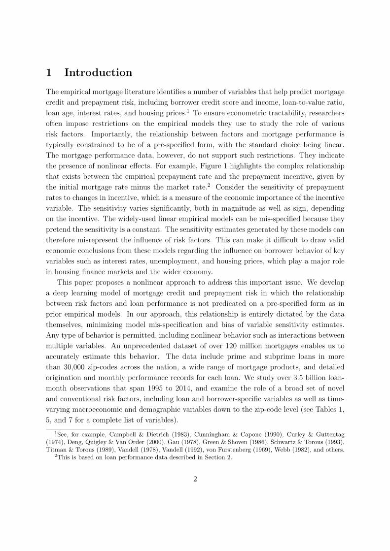
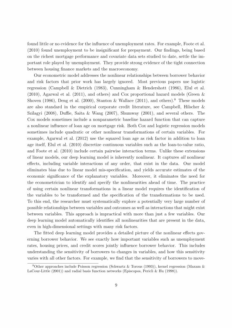
the presence of nonlinear effects. For example, Figure 1 highlights the complex relationship

that exists between the empirical prepayment rate and the prepayment incentive, given by

the initial mortgage rate minus the market rate.2 Consider the sensitivity of prepayment

rates to changes in incentive, which is a measure of the economic importance of the incentive

variable. The sensitivity varies significantly, both in magnitude as well as sign, depending

on the incentive. The widely-used linear empirical models can be mis-specified because they

pretend the sensitivity is a constant. The sensitivity estimates generated by these models can

therefore misrepresent the influence of risk factors. This can make it difficult to draw valid

economic conclusions from these models regarding the influence on borrower behavior of key

variables such as interest rates, unemployment, and housing prices, which play a major role

in housing finance markets and the wider economy.

This paper proposes a nonlinear approach to address this important issue. We develop

a deep learning model of mortgage credit and prepayment risk in which the relationship

between risk factors and loan performance is not predicated on a pre-specified form as in

prior empirical models. In our approach, this relationship is entirely dictated by the data

themselves, minimizing model mis-specification and bias of variable sensitivity estimates.

Any type of behavior is permitted, including nonlinear behavior such as interactions between

multiple variables. An unprecedented dataset of over 120 million mortgages enables us to

accurately estimate this behavior. The data include prime and subprime loans in more

than 30,000 zip-codes across the nation, a wide range of mortgage products, and detailed

origination and monthly performance records for each loan. We study over 3.5 billion loan-

month observations that span 1995 to 2014, and examine the role of a broad set of novel

and conventional risk factors, including loan and borrower-specific variables as well as time-

varying macroeconomic and demographic variables down to the zip-code level (see Tables 1,

5, and 7 for a complete list of variables).

1See, for example, Campbell & Dietrich (1983), Cunningham & Capone (1990), Curley & Guttentag(1974), Deng, Quigley & Van Order (2000), Gau (1978), Green & Shoven (1986), Schwartz & Torous (1993),Titman & Torous (1989), Vandell (1978), Vandell (1992), von Furstenberg (1969), Webb (1982), and others.

2This is based on loan performance data described in Section 2.

2

10 5 0 5 10

Original Interest Rate - National Mortgate Rate

0.00

0.01

0.02

0.03

0.04

0.05

0.06

Em

pir

ical Pre

paym

ent

Rate

Figure 1: Empirical monthly prepayment rate vs. prepayment incentive.

Our empirical analysis reveals that many variables have a highly nonlinear influence on

borrower behavior which prior work does not address. Prepayment events are especially

affected. Variable interactions, including those between more than two factors, are found

to represent a significant component of the nonlinear effects. An interaction between vari-

ables occurs when the sensitivity of loan performance to a variable also depends on one or

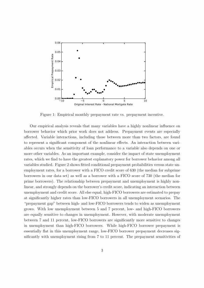
more other variables. As an important example, consider the impact of state unemployment

rates, which we find to have the greatest explanatory power for borrower behavior among all

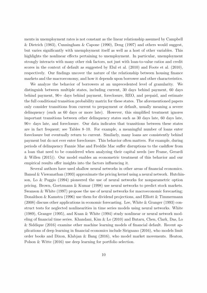
variables studied. Figure 2 shows fitted conditional prepayment probabilities versus state un-

employment rates, for a borrower with a FICO credit score of 630 (the median for subprime

borrowers in our data set) as well as a borrower with a FICO score of 730 (the median for

prime borrowers). The relationship between prepayment and unemployment is highly non-

linear, and strongly depends on the borrower’s credit score, indicating an interaction between

unemployment and credit score. All else equal, high-FICO borrowers are estimated to prepay

at significantly higher rates than low-FICO borrowers in all unemployment scenarios. The

“prepayment gap” between high- and low-FICO borrowers tends to widen as unemployment

grows. With low unemployment between 5 and 7 percent, low- and high-FICO borrowers

are equally sensitive to changes in unemployment. However, with moderate unemployment

between 7 and 11 percent, low-FICO borrowers are significantly more sensitive to changes

in unemployment than high-FICO borrowers. While high-FICO borrower prepayment is

essentially flat in this unemployment range, low-FICO borrower prepayment decreases sig-

nificantly with unemployment rising from 7 to 11 percent. The prepayment sensitivities of

3

5 6 7 8 9 10 11 12 13State Unemployment Rate

0.005

0.010

0.015

0.020

0.025

0.030

0.035

0.040Fi

tted

Prob

abilit

y of

Pre

paym

ent

FICO score 630FICO score 730

Figure 2: Fitted monthly prepayment probability vs. state unemployment.

high- and low-FICO borrowers converge as unemployment rises above 11 percent.

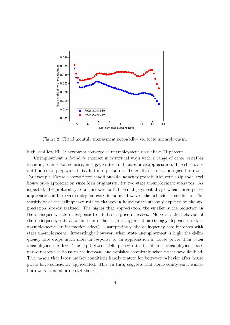
Unemployment is found to interact in nontrivial ways with a range of other variables

including loan-to-value ratios, mortgage rates, and house price appreciation. The effects are

not limited to prepayment risk but also pertain to the credit risk of a mortgage borrower.

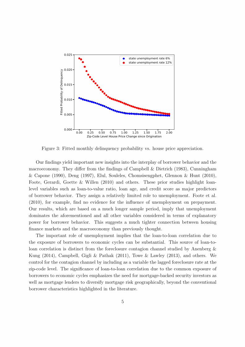
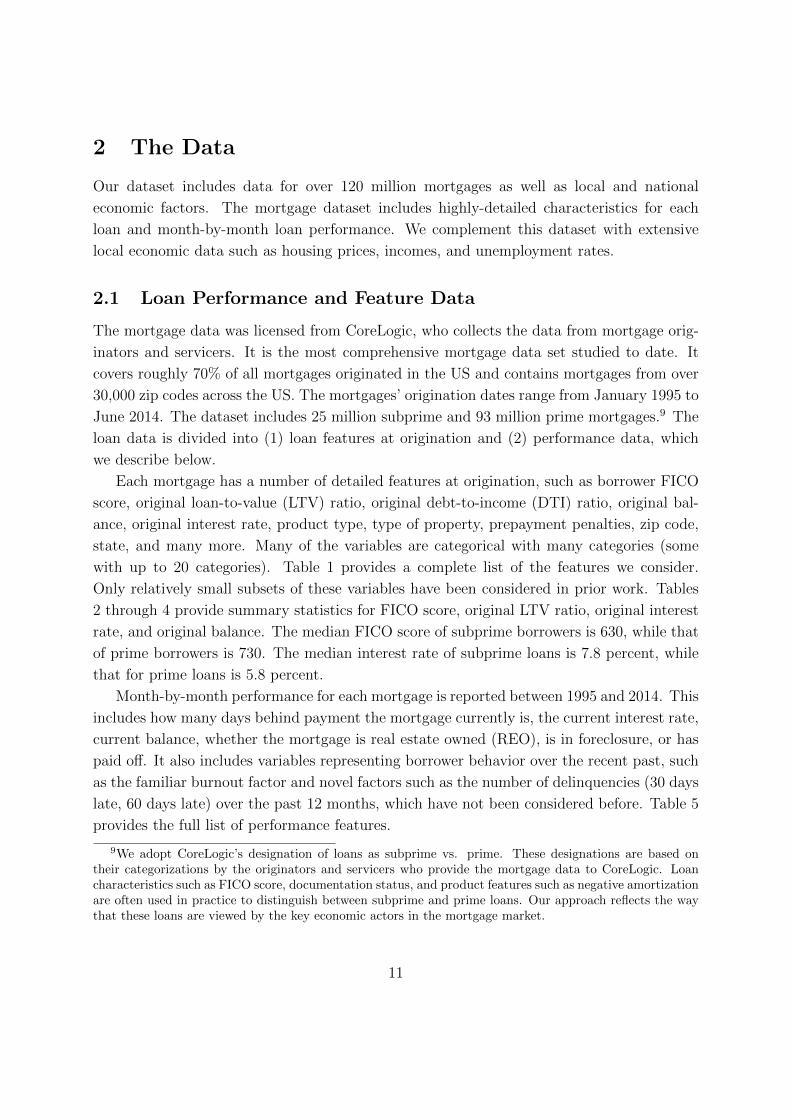
For example, Figure 3 shows fitted conditional delinquency probabilities versus zip-code level

house price appreciation since loan origination, for two state unemployment scenarios. As

expected, the probability of a borrower to fall behind payment drops when house prices

appreciate and borrower equity increases in value. However, the behavior is not linear. The

sensitivity of the delinquency rate to changes in house prices strongly depends on the ap-

preciation already realized. The higher that appreciation, the smaller is the reduction in

the delinquency rate in response to additional price increases. Moreover, the behavior of

the delinquency rate as a function of house price appreciation strongly depends on state

unemployment (an interaction effect). Unsurprisingly, the delinquency rate increases with

state unemployment. Interestingly, however, when state unemployment is high, the delin-

quency rate drops much more in response to an appreciation in house prices than when

unemployment is low. The gap between delinquency rates in different unemployment sce-

narios narrows as house prices increase, and vanishes completely when prices have doubled.

This means that labor market conditions hardly matter for borrower behavior after house

prices have sufficiently appreciated. This, in turn, suggests that home equity can insulate

borrowers from labor market shocks.

4

0.00 0.25 0.50 0.75 1.00 1.25 1.50 1.75 2.00Zip-Code Level House Price Change since Origination

0.000

0.005

0.010

0.015

0.020

0.025

Fitte

d Pr

obab

ility

of D

elin

quen

cystate unemployment rate 6%state unemployment rate 12%

Figure 3: Fitted monthly delinquency probability vs. house price appreciation.

Our findings yield important new insights into the interplay of borrower behavior and the

macroeconomy. They differ from the findings of Campbell & Dietrich (1983), Cunningham

& Capone (1990), Deng (1997), Elul, Souleles, Chomsisengphet, Glennon & Hunt (2010),

Foote, Gerardi, Goette & Willen (2010) and others. These prior studies highlight loan-

level variables such as loan-to-value ratio, loan age, and credit score as major predictors

of borrower behavior. They assign a relatively limited role to unemployment. Foote et al.

(2010), for example, find no evidence for the influence of unemployment on prepayment.

Our results, which are based on a much longer sample period, imply that unemployment

dominates the aforementioned and all other variables considered in terms of explanatory

power for borrower behavior. This suggests a much tighter connection between housing

finance markets and the macroeconomy than previously thought.

The important role of unemployment implies that the loan-to-loan correlation due to

the exposure of borrowers to economic cycles can be substantial. This source of loan-to-

loan correlation is distinct from the foreclosure contagion channel studied by Anenberg &

Kung (2014), Campbell, Gigli & Pathak (2011), Towe & Lawley (2013), and others. We

control for the contagion channel by including as a variable the lagged foreclosure rate at the

zip-code level. The significance of loan-to-loan correlation due to the common exposure of

borrowers to economic cycles emphasizes the need for mortgage-backed security investors as

well as mortgage lenders to diversify mortgage risk geographically, beyond the conventional

borrower characteristics highlighted in the literature.

5

The nonlinear nature of the relationship between unemployment and borrower behavior

entails that the sensitivity of a borrower to changes in unemployment strongly depends on the

prevailing unemployment rate as well as the borrower’s characteristics. For example, a 10%

drop in unemployment from 7% to 6.3% affects a given borrower differently than one from

10% to 9%. Moreover, due to multiple variable interactions, the effect varies very significantly

across the entire borrower population, not just across borrowers with different loan-to-value

ratios and credit scores as suggested by Elul et al. (2010) and Foote et al. (2010) in the case

of borrower default. This is important for mortgage-backed security investors, who need

to account for these effects when hedging their positions against macroeconomic volatility.

Rating agencies need to address the nonlinear behavior when assessing the exposure of

mortgage securities to adverse macroeconomic conditions. Many prior articles studying the

role of unemployment, for example Campbell & Dietrich (1983), Cunningham & Capone

(1990), Deng (1997) and others, ignore the pronounced nonlinear behavior by assuming that

the sensitivity of borrowers to changes in unemployment is constant and independent of all

other variables including borrower characteristics.

Our empirical results are based on a deep learning model for mortgage states over mul-

tiple periods. The model harnesses the unprecedented size of our sample set and the large

number of risk factors we examine (272 in total). It is designed to capture the nonlinear

relationships between variables and mortgage state probabilities present in the data. The

model distinguishes between multiple states, including current, 30 days past due, 60 days

past due, 90+ days past due, foreclosure, REO (real-estate-owned), and prepaid. It offers

likelihood estimators for the term structure of the full conditional transition probability

matrix for these states. The estimators incorporate the significant time-series variation of

the explanatory variables over the 20-year sample period as well as their future movements.

They are shown to yield superior out-of-sample predictions of multi-period mortgage risk at

the individual loan level as well as the mortgage pool level. We also demonstrate that they

enable the selection of performing mortgage investment portfolios. The tests indicate the

ability of the deep learning model to capture the stand-alone risk of a loan as well as the

substantial correlation that exists between the loans in a portfolio. The model’s predictive

accuracy suggests its usefulness for several important applications, including the valuation

of mortgage-backed securities as in Curley & Guttentag (1977), Schwartz & Torous (1989)

and Stanton & Wallace (2011).3

3The valuations generated by our model would harness the detailed data available for each of the under-lying loans. This contrasts with alternative “top-down” valuation approaches such as Schwartz & Torous(1989), McConnell & Singh (1994) and Boudoukh, Whitelaw, Richardson & Stanton (1997), who directlymodel the aggregate behavior of a pool without reference to the pool constituents.

6

Our deep learning model for mortgage state probabilities is a nonlinear extension of the

familiar logistic regression model, which is widely used in the empirical mortgage literature4

and beyond. It can be thought of as a logistic regression of recursively specified basis func-

tions that nonlinearly transform the explanatory variables and are learned from the data.

The model can also be represented by an interconnected set of input, output, and “hidden”

nodes, which is often called a neural network.5 The input nodes represent the explana-

tory variables while the output nodes represent the conditional probabilities of the different

mortgage states (current, 30 days late, prepaid, foreclosed, etc.). The hidden nodes connect

the input and output nodes, and represent the nonlinear transformations of input variables.

Given enough hidden nodes, a neural network can approximate arbitrarily well the true map-

ping between explanatory variables and conditional mortgage state probabilities.6 This of

course includes approximating nonlinear relations and interactions such as the product and

division of variables.

In particular, we examine deep neural networks, which have multiple layers of hidden

nodes. Deep architectures enable sparser representations of complex relationships than shal-

low networks with few hidden layers.7 Our fitting experiments with networks of different

depth indicate a strong preference for deeper networks, highlighting the existence of highly

nonlinear relationships and variable interactions in the mortgage data. The optimal net-

work architecture, determined via cross-validation methods, has five layers of hidden nodes,

each having between 140 and 200 nodes. We develop computationally efficient maximum

likelihood fitting algorithms that take advantage of recent advances in GPU parallel and

cloud computing. Overfitting is tightly controlled by regularization, dropout, and ensemble

modeling, and as a result is found to be insignificant.

The remainder of the introduction discusses the related literature. Section 2 examines

our dataset and performs some exploratory analyses that will inform the specification of

our deep learning model in Section 3. Section 4 discusses likelihood estimation for the deep

learning model. Section 5 reports our empirical results. Section 6 examines the out-of-sample

behavior of the deep learning model. Section 7 offers concluding remarks. There are several

technical appendices.

4See Campbell & Dietrich (1983), Cunningham & Capone (1990), and more recently, Agarwal, Amromin,Ben-David, Chomsisengphet & Evanoff (2011), Agarwal, Chang & Yavaz (2012), Jiang, Nelson & Vytlacil(2014), and Rajan, Seru & Vig (2015).

5For a broad introduction to deep learning, see White (1992) and Goodfellow, Bengio & Courville (2016).6More precisely, a neural network can approximate arbitrarily well continuous functions on compact sets,

see Hornik, Stinchcombe & White (1989) and Hornik (1991).7See Mallat (2016), Telgarsky (2016), Eldan & Shamir (2016), Bengio & LeCun (2007), and Montufar,

Pascanu, Cho & Bengio (2014).

7

1.1 Related Literature

There is a substantial empirical literature on mortgage delinquency and prepayment risk.

In early work, von Furstenberg (1969) establishes the influence on home mortgage default

rates of variables such as income, loan age, and loan-to-value ratio. Gau (1978), Vandell

(1978), Webb (1982), Campbell & Dietrich (1983) and others examine additional variables.

Commercial mortgage default is studied by Titman & Torous (1989) and Vandell (1992),

among others. Curley & Guttentag (1974) is an early study of prepayment rates. Green

& Shoven (1986) and Richard & Roll (1989) examine the influence of interest rates on

prepayments. Cunningham & Capone (1990), Schwartz & Torous (1993), and Deng (1997)

analyze the influence on default and prepayment of several loan-level and macro-economic

variables, recognizing the “competing” nature of default and prepayment events. Deng

et al. (2000) analyze the extent to which option theory can explain default and prepayment

behavior. Schwartz & Torous (1989) pioneered the use of empirical pool-level prepayment

models for the pricing of agency mortgage-backed securities. More recently, Stanton &

Wallace (2011) use empirical models of default and prepayment to price private-label MBS.

Chernov, Dunn & Longstaff (2016) estimate market-implied risk-neutral prepayment rates

and relate them to various explanatory variables.

This study of mortgage credit and prepayment risk represents a significant departure from

earlier work, in several respects. Our empirical analysis is based on an unprecedented dataset

of 120 million prime and subprime mortgages observed over the period 1995–2014. The afore-

mentioned prior work has examined much smaller samples (tens to hundreds of thousands of

loans), focusing on particular geographic regions, time periods, economic regimes, loan prod-

ucts, borrower profiles, and a limited set of loan-level and macro-economic risk factors. It is

unclear to what extent the empirical findings of these earlier studies can be generalized. Our

dataset includes about 70 percent of all US mortgages originated between 1995 and 2014,

and is the most comprehensive mortgage data set studied to date. It covers all product types,

including fixed-rate, adjustable-rate, hybrid, balloon, and other types of loans, and tracks

their performance during several economic cycles. With samples spanning two decades and

spread across over 30,000 zip codes, we are in a position to study the joint influence on

mortgage risk of a broad set of novel and conventional risk factors that describe a variety of

borrower and product characteristics as well as economic and demographic conditions down

to the zip-code level. Our results highlight the importance of the local economic conditions

that borrowers face, after controlling for the influence of the factors that prior studies have

identified as significant predictors of mortgage risk. In particular, we identify state unem-

ployment rates as the factor with the greatest explanatory power for borrower behavior.

Some prior studies, focusing on short sample periods and few controls, found unemployment

to be dominated by borrower variables (e.g., Deng (1997), Elul et al. (2010)) while others

8

found little or no evidence for the influence of unemployment rates. For example, Foote et al.

(2010) found unemployment to be insignificant for prepayment. Our findings, being based

on the richest mortgage performance and covariate data sets studied to date, settle the im-

portant role played by unemployment. They provide strong evidence of the tight connection

between housing finance markets and the macroeconomy.

Our econometric model addresses the nonlinear relationships between borrower behavior

and risk factors that prior work has largely ignored. Most previous papers use logistic

regression (Campbell & Dietrich (1983), Cunningham & Hendershott (1986), Elul et al.

(2010), Agarwal et al. (2011), and others) and Cox proportional hazard models (Green &

Shoven (1986), Deng et al. (2000), Stanton & Wallace (2011), and others).8 These models

are also standard in the empirical corporate credit literature, see Campbell, Hilscher &

Szilagyi (2008), Duffie, Saita & Wang (2007), Shumway (2001), and several others. The

Cox models sometimes include a nonparametric baseline hazard function that can capture

a nonlinear influence of loan age on mortgage risk. Both Cox and logistic regression models

sometimes include quadratic or other nonlinear transformations of certain variables. For

example, Agarwal et al. (2012) use the squared loan age as risk factor in addition to loan

age itself, Elul et al. (2010) discretize continuous variables such as the loan-to-value ratio,

and Foote et al. (2010) include certain pairwise interaction terms. Unlike these extensions

of linear models, our deep learning model is inherently nonlinear. It captures all nonlinear

effects, including variable interactions of any order, that exist in the data. Our model

eliminates bias due to linear model mis-specification, and yields accurate estimates of the

economic significance of the explanatory variables. Moreover, it eliminates the need for

the econometrician to identify and specify the nonlinearities ahead of time. The practice

of using certain nonlinear transformations in a linear model requires the identification of

the variables to be transformed and the specification of the transformations to be used.

To this end, the researcher must systematically explore a potentially very large number of

possible relationships between variables and outcomes as well as interactions that might exist

between variables. This approach is impractical with more than just a few variables. Our

deep learning model automatically identifies all nonlinearities that are present in the data,

even in high-dimensional settings with many risk factors.

The fitted deep learning model provides a detailed picture of the nonlinear effects gov-

erning borrower behavior. We see exactly how important variables such as unemployment

rates, housing prices, and credit scores jointly influence borrower behavior. This includes

understanding the sensitivity of borrowers to changes in variables, and how this sensitivity

varies with all other factors. For example, we find that the sensitivity of borrowers to move-

8Other approaches include Poisson regression (Schwartz & Torous (1993)), kernel regression (Maxam &LaCour-Little (2001)) and radial basis function networks (Episcopos, Pericli & Hu (1998)).

9

ments in unemployment rates is not constant as the linear relationship assumed by Campbell

& Dietrich (1983), Cunningham & Capone (1990), Deng (1997) and others would suggest,

but varies significantly with unemployment itself as well as a host of other variables. This

highlights the nonlinear effects pertaining to unemployment. In particular, unemployment

strongly interacts with many other risk factors, not just with loan-to-value ratios and credit

scores in the context of default as suggested by Elul et al. (2010) and Foote et al. (2010),

respectively. Our findings uncover the nature of the relationship between housing finance

markets and the macroeconomy, and how it depends upon borrower and other characteristics.

We analyze the behavior of borrowers at an unprecedented level of granularity. We

distinguish between multiple states, including current, 30 days behind payment, 60 days

behind payment, 90+ days behind payment, foreclosure, REO, and prepaid, and estimate

the full conditional transition probability matrix for these states. The aforementioned papers

only consider transitions from current to prepayment or default, usually meaning a severe

delinquency (such as 60 days or more late). However, this simplified treatment ignores

important transitions between other delinquency states such as 30 days late, 60 days late,

90+ days late, and foreclosure. Our data indicates that transitions between these states

are in fact frequent; see Tables 8–10. For example, a meaningful number of loans enter

foreclosure but eventually return to current. Similarly, many loans are consistently behind

payment but do not ever enter foreclosure. This behavior often matters. For example, during

periods of delinquency Fannie Mae and Freddie Mac suffer disruptions to the cashflow from

a loan that need to be considered when analyzing their capital needs (see Frame, Gerardi

& Willen (2015)). Our model enables an econometric treatment of this behavior and our

empirical results offer insights into the factors influencing it.

Several authors have used shallow neural networks in other areas of financial economics.

Bansal & Viswanathan (1993) approximate the pricing kernel using a neural network. Hutchin-

son, Lo & Poggio (1994) pioneered the use of neural networks for nonparametric option

pricing. Brown, Goetzmann & Kumar (1998) use neural networks to predict stock markets.

Swanson & White (1997) propose the use of neural networks for macroeconomic forecasting;

Donaldson & Kamstra (1996) use them for dividend projections, and Elliott & Timmermann

(2008) discuss other applications in economic forecasting. Lee, White & Granger (1993) con-

struct tests for neglected nonlinearities in time series models using neural networks. White

(1989), Granger (1995), and Kuan & White (1994) study nonlinear or neural network mod-

eling of financial time series. Khandani, Kim & Lo (2010) and Butaru, Chen, Clark, Das, Lo

& Siddique (2016) examine other machine learning models of financial default. Recent ap-

plications of deep learning in financial economics include Sirignano (2016), who models limit

order books and Dixon, Klabjan & Bang (2016), who model market movements. Heaton,

Polson & Witte (2016) use deep learning for portfolio selection.

10

2 The Data

Our dataset includes data for over 120 million mortgages as well as local and national

economic factors. The mortgage dataset includes highly-detailed characteristics for each

loan and month-by-month loan performance. We complement this dataset with extensive

local economic data such as housing prices, incomes, and unemployment rates.

2.1 Loan Performance and Feature Data

The mortgage data was licensed from CoreLogic, who collects the data from mortgage orig-

inators and servicers. It is the most comprehensive mortgage data set studied to date. It

covers roughly 70% of all mortgages originated in the US and contains mortgages from over

30,000 zip codes across the US. The mortgages’ origination dates range from January 1995 to

June 2014. The dataset includes 25 million subprime and 93 million prime mortgages.9 The

loan data is divided into (1) loan features at origination and (2) performance data, which

we describe below.

Each mortgage has a number of detailed features at origination, such as borrower FICO

score, original loan-to-value (LTV) ratio, original debt-to-income (DTI) ratio, original bal-

ance, original interest rate, product type, type of property, prepayment penalties, zip code,

state, and many more. Many of the variables are categorical with many categories (some

with up to 20 categories). Table 1 provides a complete list of the features we consider.

Only relatively small subsets of these variables have been considered in prior work. Tables

2 through 4 provide summary statistics for FICO score, original LTV ratio, original interest

rate, and original balance. The median FICO score of subprime borrowers is 630, while that

of prime borrowers is 730. The median interest rate of subprime loans is 7.8 percent, while

that for prime loans is 5.8 percent.

Month-by-month performance for each mortgage is reported between 1995 and 2014. This

includes how many days behind payment the mortgage currently is, the current interest rate,

current balance, whether the mortgage is real estate owned (REO), is in foreclosure, or has

paid off. It also includes variables representing borrower behavior over the recent past, such

as the familiar burnout factor and novel factors such as the number of delinquencies (30 days

late, 60 days late) over the past 12 months, which have not been considered before. Table 5

provides the full list of performance features.

9We adopt CoreLogic’s designation of loans as subprime vs. prime. These designations are based ontheir categorizations by the originators and servicers who provide the mortgage data to CoreLogic. Loancharacteristics such as FICO score, documentation status, and product features such as negative amortizationare often used in practice to distinguish between subprime and prime loans. Our approach reflects the waythat these loans are viewed by the key economic actors in the mortgage market.

11

The dataset covers various mortgage products including, for example, fixed rate mort-

gages, adjustable rate mortgages (ARMs), hybrid mortgages, and balloon mortgages.10 Table

6 lists the fraction of mortgages in each product category. The vast majority of the prime

mortgages are fixed-rate (86%), followed by ARMs (9%) and hybrids (4%). 48% of the

subprime mortgages are fixed-rate, 29% are ARMs, and 9% are hybrids. Prior work has

typically focused on a particular product such as fixed-rate loans.

Every monthly observation from each of the loans constitutes a data sample. After clean-

ing the data as described in Appendix A, there are roughly 3.5 billion monthly observations

remaining. 90% of the samples are for prime mortgages and the remaining are for subprime.

The samples cover the period January, 1995 to May, 2014. Each sample (i.e., monthly obser-

vation) has 272 explanatory variables as well as the outcome for that month (i.e., if the loan

is current, 30 days delinquent, 60 days delinquent, etc.). Of these explanatory variables, 234

are loan-level feature and performance variables, 25 are indicators for missing features (see

Appendix A), and 13 are economic variables which are introduced next.

2.2 Local and National Economic Factors

We complement the loan-level data described above by data for local and national economic

factors which may influence loan performance. Table 7 lists the factors we consider. We use

a mortgage’s zip code to match a mortgage with local factors such as the monthly housing

price in that zip code. Housing prices are obtained from Zillow and the Federal Housing

Administration (FHA). Zillow housing prices are at the five-digit zip code level and cover

roughly 10,000 zip codes. In order to cover less populated areas not covered by the Zillow

dataset, we also include FHA housing prices which cover all three-digit zip codes. The

monthly national mortgage rate is obtained from Freddie Mac, is also included as a factor.11

Unemployment rates at the county level for each year and state unemployment rates for each

month are obtained from the Bureau of Labor Statistics.12 Our data also includes the yearly

median income in each zip code, which was acquired from the data provider Powerlytics.

Moreover, we include a dummy variable for the vintage year. Finally, the granular geographic

data is used to construct the lagged default and prepayment rates in each zip code across

the US, using the historical data for all mortgages. The inclusion of these rates allows us

10A fixed rate mortgage has constant interest and principal payments over the lifetime of the mortgage.An ARM has interest payments which fluctuate with some other index interest rate (such as the Treasuryrate) plus some fixed margin. A hybrid mortgage has a period with a fixed rate followed by a period withan adjustable rate. Hybrid mortgages can also have other features such as interest rate caps. A balloonmortgage only partially amortizes; a portion of the loan principal is due at maturity.

11The monthly national mortgage rate used in this paper is an average of 30 year fixed rates for first-lienprime conventional conforming home purchase mortgages with a loan-to-value of 80 percent.

12We match counties and zip codes in order to associate each mortgage with a particular county.

12

to capture a potential contagion effect where defaults of mortgages increase the likelihood

of default for nearby surviving mortgages. Such a feedback mechanism has been supported

by several recent empirical papers; see Agarwal, Ambrose & Yildirim (2015), Anenberg &

Kung (2014), Campbell et al. (2011), Harding, Rosenblatt & Yao (2009), Lin, Rosenblatt &

Yao (2009), Towe & Lawley (2013), and others.

2.3 Mortgage States and Transitions

Mortgages are allowed to transition between 7 states: current, 30 days delinquent, 60 days

delinquent, 90+ days delinquent, foreclosed, REO, and paid off. X days delinquent simply

means the mortgage borrower is X days behind on their payments to the lender. We use

the standard established by the Mortgage Bankers Association of America for determining

the state of delinquency. A mortgage is determined to be 1 month delinquent if no payment

has been made by the last day of the month and the payment was due on the first day of

the month. REO stands for real estate owned property. When a foreclosed mortgage does

not sell at auction, the lender or servicer will assume ownership of the property. Paid off

can occur from a mortgage prepaying, maturing (this is very rare since the mortgages in the

dataset are almost entirely originated in the 2000s), a shortsale, or a foreclosed mortgage

being sold at auction to a third party (this is again rare in comparison to prepayments,

which form the bulk of the paid off events in the dataset).13

The state transition matrix for the monthly transitions between states are given in Tables

8, 9, and 10 for subprime, prime, and all mortgages, respectively. The state transition matrix

records the empirical frequency of the different types of transitions between states. For the

calculation of these transition matrices and the remainder of the paper, REO and paid off

are treated as absorbing states.14 That is, we stop tracking the mortgage after the first

time it enters REO or paid off. The transition matrices highlight that mortgages frequently

transition back and forth between current and various delinquency states. Disruptions in

cashflow to the lender or servicer are common due to the mortgage being behind payment.

Similarly, even loans that are extremely delinquent may return to current; the transition

from foreclosed back to current is actually a relatively frequent occurrence.15 A foreclosure

could get cured via paying the outstanding balance, there could be a pre-auction sale that

covers all or some of the amount outstanding, or there could be a sale at the foreclosure

13A foreclosed loan sold at auction may or may not be sold for a loss. The CoreLogic dataset makes nodistinction between the two events.

14In some states in the USA there are laws that allow the mortgage borrower to reclaim their mortgageeven after it has entered REO. However, such events are exceedingly rare.

15Many servicers follow a “dual path servicing approach” where they foreclose on the borrower as a threatin order to force the borrower to become current on payments.

13

auction that covers all or some of the amount outstanding. Any of these will register as a

foreclosure to paid off transition. Mortgages can also transition directly from current, 30

days delinquent, 60 days delinquent, or 90+ days delinquent to REO via a “deed in lieu of

foreclosure”.16

2.4 Nonlinear Effects

The relationships between state transition rates and explanatory variables (i.e., loan-level

features and economic factors) are often highly nonlinear. For instance, Figure 1 shows the

empirical monthly prepayment rate versus the “incentive to prepay”, initial interest rate

minus national mortgage rate.17 A higher interest rate on the loan (as compared to the

national mortgage rate) should encourage the borrower to seek better terms by refinancing

the loan, implying that an upward trend should be observed in the graph. The observed

data, however, point to more complicated underlying mechanisms, such as the presence of

prepayment penalties or the lack of refinancing options due to other factors such as low FICO

scores. For example, a low initial interest rate may have been facilitated by prepayment

penalties or points upfront, which will be disincentives to prepaying. Figure 4 shows the

empirical monthly prepayment rate versus the FICO score. The propensity to prepay is less

for borrowers with lower FICO scores but it plateaus once the score crosses a threshold of

about 500 points. Figure 5 shows the empirical monthly prepayment rate versus the time

since origination. Several spikes in the rate occur at 1, 2, and 3 years. These might be due

to the expiration of prepayment penalties or adjustable rate and hybrid mortgages having

rate resets. Many of the subprime mortgages started with low teaser rates and would later

jump to higher rates; borrowers would refinance to avoid these rate jumps. Figure 6 plots

the empirical monthly prepayment rate versus the loan-to-value (LTV) ratio. One should

expect this curve to have a downward slope since a loan with high LTV will have lesser

opportunities to refinance due to a large loan amount relative to the value of the asset.

Each of these charts displays significant nonlinear relationships between the variable and the

empirical prepayment rate. This reinforces the need for a loan performance model that is

capable of addressing such relationships.

16A “deed in lieu of foreclosure” is when the loan is in default and the borrower gives ownership of theproperty directly to the lender, thereby forgoing foreclosure.

17A more accurate proxy for the incentive to prepay would be the current interest rate minus the mortgagerate. However, a large portion of the mortgages in the dataset are missing the current interest rate so theinitial interest rate was used instead to achieve greater coverage.

14

3 Deep Learning Model

We propose a dynamic nonlinear model for the performance of a pool of mortgage loans

over time. We adopt a discrete-time formulation for periods 0, 1, . . . , T (e.g., months).18 We

enumerate the possible mortgage states (current, 30 days delinquent, etc.), and let U ⊂ Ndenote the set of these states. The variable Un

t ∈ U prescribes the state of the n-th mortgage

at time t after origination. A mortgage will transition between the various states over its

lifetime. For instance, a trajectory of the state process might be:

Un0 = 1 (current), Un

1 = 2 (30 days late), Un2 = 1 (current), Un

3 = 5 (paid off).

We allow the dynamics of the state process to be influenced by a vector of explanatory

variables Xnt ∈ RdX which includes the mortgage state Un

t . In our empirical implementation,

Xnt represents the original and contemporary loan-level features in Tables 1 and 5, and the

contemporary local and national economic factors in Table 7.19 We specify a probability

transition function hθ : U × RdX → [0, 1] satisfying

P[Unt = u | Ft−1] = hθ(u,X

nt−1), u ∈ U , (1)

where θ is a parameter to be estimated. Equation (1) gives the marginal conditional prob-

ability for the transition of the n-th mortgage from its state Unt−1 at time t − 1 to state

u at time t given the explanatory variables Xnt−1. The family of conditional probabilities

give a conditional transition probability matrix, which is the conditional counterpart of the

empirical transition matrix reported in Table 10. Note that the conditional probabilities will

be correlated across loans if Xnt−1 includes variables that are common to several loans. This

formulation allows us to capture loan-to-loan correlation due to geographic proximity and

common economic factors.

We propose to model the transition function hθ by a neural network. Let g denote the

standard softmax function:

g(z) =

(ez1∑Kk=1 e

zk, . . . ,

ezK∑Kk=1 e

zk

), z = (z1, . . . , zK) ∈ RK , (2)

where K = |U|.20 The vector output of the function g is a probability distribution on U .

18We fix a probability space (Ω,F ,P) and an information filtration (Ft)t=0,1,...,T .19As usual, categorial variables are encoded in terms of indicator functions (dummy variables).20Certain transitions are not allowed in the dataset (e.g., current to 60 days delinquent). Although such

a transition is theoretically allowed in the formulation (2), the transition probabilities of transitions whichdo not occur in the dataset will be driven to zero during training.

15

The specification hθ(u, x) = (g(Wx+ b))u, where W ∈ RK × RdX , b ∈ RK , and Vu is the

u-th element of the vector V , gives a logistic regression model.21 Here, the link function

g takes a linear function of the covariates x as its input. The output hθ(u, x) varies only

in the constant direction given by W . A standard approach to achieve a more complex

model with greater flexibility is to replace x in the specification with a nonlinear function

of x. Let φ : RdX → Rdφ and set hθ(u, x) = (g(Wφ(x) + b))u, where W ∈ RK × Rdφ and

b ∈ Rdφ . This is a logistic regression of the basis functions φ = (φ1, . . . , φdφ). For instance,

polynomials, step functions, or splines could be chosen as the basis functions. It is important

to recognize that, even if the basis functions are nonlinear in the input space, the logistic

regression model remains a link function of a model which is linear in the parameters θ. The

logistic model may perform poorly if the chosen basis functions are not appropriate for the

problem. Instead of fixing a set of basis functions φ ahead of time, a neural network learns

these feature functions directly from the data. The function φ is replaced by a parameterized

function φθ where θ is estimated from data. A neural network is composed of a sequence of

nonlinear operations (or “layers”). Each operation takes the output from the previous layer

and applies (1) a linear function and then (2) an element-wise nonlinearity. As a whole, a

neural network is a flexible function, highly nonlinear in the parameters, which can learn the

best feature functions φθ for the problem.

Define the nonlinear transformation φθ(x) as hθ,L−1(x). A multi-layer neural network

repeatedly passes linear combinations of learned basis functions through simple nonlinear

link functions to produce a highly nonlinear function. Formally, the output hθ,l : RdX → Rdl

of the l-th layer of the neural network is:

hθ,l(x) = gl(W>l hθ,l−1(x) + bl), (3)

where Wl ∈ Rdl × Rdl−1 , bl ∈ Rdl , and hθ,0(x) = x. For l = 1, . . . , L − 1, the nonlinear

transformation gl(z) = (σ(z1), . . . , σ(zdl)) for z = (z1, . . . , zdl) ∈ Rdl and gL(z) is given by

the softmax function g(z) defined in (2). Note that dL = K = |U|. The function σ : R→ Ris a simple nonlinear link function; typical choices are sigmoidal functions, tanh, and rectified

linear units (i.e., max(x, 0)). The final output of the neural network is given by:

hθ(u, x) = (hθ,L(x))u = (g(W>L hθ,L−1(x) + bL))u. (4)

The parameter specifying the neural network is

θ = (W1, . . . ,WL, b1, . . . , bL), (5)

21Campbell & Dietrich (1983), Cunningham & Hendershott (1986), Elul et al. (2010), Agarwal et al.(2011), and many others use logistic regression models to analyze mortgage performance.

16

where L is the number of layers in the neural network. At each layer l, the output hθ,l(x) is

a simple nonlinear link function gl of a linear combination of the nonlinear basis functions

hθ,l−1(x), where the nonlinear basis function hθ,l−1(x) must be learned from data via the

parameter θ. The output hθ,l(x) from the l-th layer of the neural network becomes the basis

function for the (l + 1)-th layer.

The layers between the input at layer l = 0 and the output at layer l = L are referred

to as the hidden layers. Thus, the neural network hθ has L − 1 hidden layers. A neural

network with zero hidden layers (L = 1) is a logistic regression model. More hidden layers

allow for the neural network to fit more complex patterns. Each subsequent layer extracts

increasingly nonlinear features from the data. Early layers pick up simpler features while

later layers will build upon these simple features to produce more complex features. The

l-th layer has dl outputs where each output is an affine transformation of the output of layer

l − 1 followed by an application of the nonlinear function σ. This composition of functions

is called a hidden unit, or simply, a unit, since it is the fundamental building block of neural

networks. The number of units in the l-th layer is dl and the complexity of any layer (and the

complexity of the features it can extract) increases with the number of units in that layer.

Thus, increased complexity can be achieved by increasing either the number of units or the

number of layers. Given enough units, a neural network can approximate arbitrarily well

continuous functions on compact sets (Hornik 1991). This of course includes approximating

arbitrarily well interactions such as the product and division of features. The advantage of

more layers (as opposed to simply adding more units to existing layers) is that the later

layers learn features of greater complexity by utilizing features of the lower layers as their

inputs. Moreover, deep neural networks, i.e., networks with three or more hidden layers,

typically need exponentially fewer units than shallow networks or logistic regressions with

basis functions; see Bengio & LeCun (2007) and Montufar et al. (2014).22

(1) is a dynamic model and therefore gives transition probabilities between the states

over multiple periods (2 month, 6 month, 1 year, etc.). The transition probability matrix for

1-month ahead transitions is specified by the transition function in (1). The transition prob-

ability matrix for t-months ahead is simply the expectation of the product of the transition

probability matrices at months 0, 1, . . . , t− 1. Note that the transition probability matrices

at months t = 1, 2, . . . , t− 1 are random due to their dependence on the random covariates

Xnt . To compute these expectations, a time-series model for Xn

t needs to be formulated

and Monte Carlo samples from Xnt need to be generated. An alternate approach, which is

advantageous for reducing the computational burden and can be accurate for shorter time

horizons, is that the economic covariates in Xnt are frozen at t = 0. That is, only the state

22The number of layers and the number of neurons in each layer, along with other hyperparameters of themodel, are chosen by the standard approach of cross-validation. Section C provides the details.

17

of the mortgage and deterministic elements of Xnt (e.g., the balance of a fixed rate mortgage

and time to maturity) are allowed to evolve over time. Then, the transition probability

matrix for a horizon t > 1 is the product of the deterministic transition probability matrices

at months 0, 1, . . . , t− 1. The two approaches are implemented in Section 5.23

Our formulation captures loan-to-loan correlation due to geographic proximity and com-

mon economic factors. Pool-level quantities, such as the distribution of the prepayment rate

for a given pool, can also be computed via standard Monte Carlo simulation. The cashflow

from a pool is the sum of the cashflows from the individual loans. Thus, one simply needs

to simulate all of the individual loans based on the fitted model and then aggregate the

individual cashflows.24 If the economic covariates are frozen at time t = 0, the pool-level

distribution can be approximated in closed-form via a Poisson approximation or the central

limit theorem. Such approximations are accurate (for the distribution where covariates are

frozen) even for pools with only a few hundred loans.

We have considered alternative model architectures. For instance, one could individually

model transitions from each particular initial state with a neural network; such an approach

would require fitting K different neural networks. Another approach would be to have

separate models for each product (fixed-rate vs. ARM, etc.) or borrower class (prime

vs. subprime). Clearly, our neural network architecture is more parsimonious, which is a

desirable characteristic. However, in addition to parsimony, there is a statistical motive for

our architecture. Neural networks learn via their hidden layers recognizing, and abstracting,

nonlinear features from the data (i.e., nonlinear functions of the initial input). Different

transitions may strongly depend upon the same nonlinear features. Similarly, different types

of products are likely to depend on some of the same nonlinear features. For instance, it is

likely that there are many similar factors driving the transitions current → paid off and 30

days delinquent → paid off. In our neural network architecture, all transitions are modeled

by the same neural network, which has the advantage that more data can be used to better

estimate the nonlinear factors which drive multiple types of transitions.

4 Likelihood Estimation

This section discusses the estimation of the parameter (5) specifying the deep learning model

by the method of maximum likelihood. We are given observations of Xt = (X1t , . . . , X

Nt )

23An alternative approach to the dynamic model (1) is to fit a model for each different time horizon, asin Campbell et al. (2008). Many static models could be fitted for each of the time horizons (1 month, 2months, 6 months, 1 year, 1.5 years, 2 years, etc.). Fitting so many models is computationally expensiveand the two approaches mentioned above do not incur this cost.

24Large portfolios can be rapidly simulated using methods from Sirignano & Giesecke (2015). Fast optimalselection of loan portfolios can be performed using methods from Sirignano, Tsoukalas & Giesecke (2016).

18

at each time t = 0, . . . , T where N is the number of mortgages which are observed. We let

Xnt = (Un

t , LNt , V

nt ), where Un

t ∈ U is the state of the n-th mortgage, and Lnt includes the

lagged default and prepayment rates in the zip code of the n-th mortgage.25 The vector

V nt ∈ RdY includes the remaining contemporary local and national economic factors in Table

7, as well as the original and contemporary loan-level features in Tables 1 and 5. We make the

standard assumption26 that the variables V nt are exogenous in the sense that the law of V =

(V0, . . . , VT ), where Vt = (V 1t , . . . , V

Nt ) does not depend on the parameter θ specifying the

law of the observed mortgage states U = (U0, . . . , UT ), where Ut = (U1t , . . . , U

Nt ). Therefore,

the likelihood problem for V can be treated separately from that for U .

Although the model framework (1) is a dynamic model where the function hθ may assume

a very complicated form, the likelihood of the observed states U takes an analytical form.

The likelihood of U depends only on the observed value of V and is independent of V ’s

exact form or parameterization since V is exogenous. Letting L = (L0, . . . , LT ) and writing

informally, the log-likelihood function for θ given V is

LT,N(θ) = logPθ[U,L|V

]= logPθ

[L|U, V

]Pθ[U |V

]= logPθ

[U |V

],

where we use the fact that Pθ[L|U, V

]= 1 since Lt = (L1

t , . . . , LNt ) is a deterministic function

of U0, . . . , Ut. Under the standard assumption that the variables U1t , . . . , U

Nt are conditionally

independent given Xt−1, we have27

LT,N(θ) =T∑

t=1

logPθ[Ut∣∣Ut−1, Vt−1

]=

T∑

t=1

N∑

n=1

logPθ[Unt

∣∣Unt−1, V

nt−1

]

=N∑

n=1

T∑

t=1

log hθ(Unt , X

nt−1).

A maximum likelihood estimator (MLE) θ = θT,N for the parameter θ satisfies

θT,N ∈ arg maxθ∈ΘLT,N(θ). (6)

The asymptotic properties of the MLEs have been studied before. Under certain conditions,

the estimators are consistent and asymptotically normal; see White (1989a) and White

(1989b). Sussmann (1992) and Albertini & Sontag (1993) study identifiability.

Neural networks tend to be low-bias, high-variance models. We use several methods to

25In general, Lnt could include any variables describing the aggregate lagged performance of the mortgages.

26See Duffie et al. (2007), Campbell et al. (2008), and many others.27This expression assumes that every mortgage is originated at time t = 0. The modification for the case

where mortgages have different origination dates is straightforward.

19

address overfitting, including regularization, dropout, and ensemble modeling. A standard

`2 regularization term is included in the objective function in addition to the log-likelihood

LT,N(θ). The `2 term represents the sum of the squares of the parameters. Secondly, we use

dropout in each of the layers. Dropout is a widely-used technique in deep learning that has

proven to be very successful; see Srivastava, Hinton, Krizhevsky & Sutskever (2014). Dur-

ing fitting, hidden units are randomly removed from the network. This prevents complex

“fictitious” relationships forming between different neurons since neuron i cannot depend

upon neuron j being present. Finally, we also build an ensemble of neural networks. This

simply means that we fit a set of randomly initialized neural networks on datasets obtained

by bootstrapping from the original datasets. Typically, each neural network reaches a dif-

ferent local minimum due to each being trained with a different random initial starts and

random sequence of bootstrapped samples. Variance (i.e., overfitting) of an individual neural

network’s prediction can be reduced by taking the prediction as the average of the neural

networks’ predictions. The averaged prediction, or ensemble prediction, has lower variance

since the idiosyncratic variance for each neural network is averaged out.

Appendix B discusses the implementation of the MLE. We develop fitting algorithms

that can deal very efficiently with the large number of samples and explanatory variables we

observe. The algorithms harness recent advances in GPU parallel computing and run on a

cluster of Amazon Web Services nodes.

Appendix C details our cross-validation approach to the selection of the hyperparameters,

which include the number of layers and number of neurons per layer, the type of the activation

function σ, the size of the regularization penalty, and several other parameters governing the

fitting algorithm (see Appendix B). The optimal network architecture has five hidden layers,

with 200 units in the first hidden layer and 140 units in each subsequent one. The rectified

linear unit activation function σ(x) = max(0, x) was found to yield better performance and

faster convergence than the sigmoid σ(x) = 1/(1 + e−x).

The training set includes all the data before May 1, 2012. The validation set, which is

used for the selection of hyperparameters (see Appendix C), is May 1, 2012 until October

31, 2012. Once the hyperparameters are chosen, the model is re-fitted on the combined

training and validation sets. The final trained model is then tested out-of-sample on the

test set, which is from November 1, 2012 until May 31, 2014. All explanatory variables are

normalized by their means and standard deviations (which are calculated using data only

from the training set).

20

5 Empirical Results

The fitted deep learning model is used to understand the relationship between explanatory

factors and borrower behavior. Our analysis shows that many highly nonlinear relationships

exist. Furthermore, borrower behavior is found to have nontrivial dependencies on the

nonlinear interaction between multiple factors.

5.1 Explanatory Power of Variables

We begin by studying the explanatory power of the different factors for the behavior of

borrowers. To this end we consider the behavior of the out-of-sample negative average log-

likelihood with respect to changes to the composition of the set of factors. The negative

average log-likelihood 1NLT,N(θ) is a standard measure of fit, which is sometimes called the

cross-entropy error or simply the loss. We measure by how much the loss increases when a

variable is removed as an explanatory variable. Variables that have large explanatory power,

and whose information is not also largely contained in the other remaining covariates, will

produce large increases in the loss if they are removed.

Table 11 reports the results.28 The state unemployment rate is the variable with by far

the highest explanatory power among all variables, emphasizing the importance of local eco-

nomic conditions for borrower behavior. Standard loan-level variables such as credit score

and loan-to-value ratio, which were highlighted by Campbell & Dietrich (1983), Cunningham

& Capone (1990), Curley & Guttentag (1974), and others as major predictors of borrower

behavior, have less explanatory power. This finding suggests a much tighter connection

between housing finance markets and the macroeconomy than previously thought. Earlier

studies have assigned a relatively limited role to unemployment, see Campbell & Dietrich

(1983), Cunningham & Capone (1990), Deng (1997), Elul et al. (2010), Foote et al. (2010)

and others. Relative to our analysis, these earlier studies are based on much shorter sam-

ple periods, selected loan products (such as 30 year fixed-rate loans) and borrower profiles

(such as prime borrowers), and much smaller samples. Thus, these earlier findings are not

necessarily inconsistent with ours. However, our results provide a more definitive picture

regarding the role of unemployment than prior results because our results are based on an

unprecedented sample that spans several economic cycles over two decades.

The dominant role of unemployment suggests that the loan-to-loan correlation due to

the exposure of borrowers to economic cycles can be substantial. This source of loan-to-loan

correlation is distinct from the foreclosure contagion channel studied by Anenberg & Kung

28For clarity, we exclude from Table 11 the variable representing the current state as well as the dummiesrepresenting missing values (see Appendix A).

21

(2014), Campbell et al. (2011), Towe & Lawley (2013), and others.29 Contagion entails

a foreclosure having negative spillover effects on neighboring properties that increase the

likelihood of additional foreclosures. We control for the contagion channel by including the

lagged default rate for prime and subprime borrowers at the zip-code level as explanatory

variables (see Section 2.2). The results in Table 11 suggest that these variables have some

explanatory power, which is consistent with the existence of a contagion channel. The

fact that unemployment plays a critical role even after controlling for the contagion channel

provides evidence for the prevalence of additional loan-to-loan correlation due to the exposure

of borrowers to the local economy. This, in turn, emphasizes the need for mortgage-backed

security investors to diversify loan risk geographically, beyond the conventional borrower

characteristics highlighted in the literature.

5.2 Economic Significance of Variables

We now turn to analyzing the economic significance of the different explanatory factors for

borrower behavior. The economic significance of a particular variable is measured by the

magnitude of the derivative of a fitted transition probability with respect to the variable

(averaged over the data). The derivative is over a representative sample drawn from the

dataset rather than a single point. Specifically, we calculate the sensitivity (with respect to

j-th variable) of the fitted probability for a transition from state u to v as:

E[∣∣ ∂∂xj

hθ(V,X)∣∣∣∣∣∣V = v, U = u

]. (7)

A sensitivity of value z for a given variable means that the probability for a transition from

state u to v will approximately change (in magnitude) by z∆ if that variable is changed by a

small amount ∆. As explained in Appendix D, the sensitivity (7) can be estimated directly

from the dataset and the fitted model.

In our model formulation, the sensitivity is governed by multiple model parameters that

represent the nonlinear connections between a variable and a transition probability. It is

instructive to contrast that with the linear formulations widely used in earlier studies of

borrower behavior (see the references in Section 1.1). In the case of a linear model, a single

coefficient governs the sensitivity. When nonlinear relations are present, as in our data

(see Section 5.3 below), these coefficients/sensitivities can severely misrepresent the true

economic significance of variables.30

29See Azizpour, Giesecke & Schwenkler (2017) for a discussion of the sources of loan-to-loan correlation.30To see this, consider the linear regression f(x;α, β) = α+ βx fitted to data produced from the function

y = x2 on x ∈ [−1, 1]. The least-squares estimators are α = 13 and β = 0. This suggests that there is no

relationship between y and the covariate x. However, clearly there is a very strong relationship, which would

22

Table 12 reports sensitivities for a transition from current to paid off (i.e., prepayment).

The sensitivities indicate the strong economic significance for prepayment of original and

current outstanding loan balance.31 Other economically significant variables include origi-

nal interest rate, interest rate differentials, house price appreciation, loan age, FICO score,

lagged prepayment rates, and state unemployment.32 The importance of loan balance vari-

ables is interesting in light of earlier studies of prepayment such as Green & Shoven (1986),

Cunningham & Capone (1990) and Richard & Roll (1989). These studies focus on the influ-

ence of interest rate differentials, premium burnout, loan age, LTV ratio and several other

variables, all of which are included in our analysis. Our results indicate that loan balance

variables in fact overshadow all those previously considered variables in terms of economic

significance. Our results also firmly establish the economic significance of unemployment, a

variable which earlier studies such as Cunningham & Capone (1990) and Foote et al. (2010)

found to have no significant influence on prepayment.33

Table 13 reports sensitivities for a transition from current to 30 days delinquent.34 What

stands out is the significant role of variables that describe borrower behavior over the recent

past. These variables include the number of delinquencies (30, 60, and 90+ days late) over

the past year as well as the number of times current over the past year. The number of times

the borrower was 30 days delinquent in the last year dominates all other variables in terms

of economic significance for a transition from current to 30 days delinquent. The strong

influence of these variables indicates that borrower behavior is strongly path dependent.

Prior work on mortgage default risk such as von Furstenberg (1969), Gau (1978), Vandell

(1978), Webb (1982), Campbell & Dietrich (1983), Elul et al. (2010), Foote et al. (2010)

has not analyzed the influence of path-dependent borrower behavior variables, and instead

focused on the role of standard loan and borrower characteristics such as FICO score, interest

rates, and LTV ratios. Our results suggest that these standard variables are less influential

predictors of mortgage delinquency than previously thought.

have been identified if a nonlinear model (such as a neural network) was used.31We compare the sensitivities implied by the linear logistic regression model (i.e., a 0-layer network)

with those in Table 12 (the values are available upon request). The logistic regression model significantlyunderstates the sensitivity and hence economic importance of original and current outstanding loan balance,and overstates the sensitivity for the interest rate and interest rate differentials. Our analysis in Section 5.3below shows that prepayment has a nonlinear relationship with all these variables. A linear model such aslogistic regression can produce inaccurate sensitivities for such nonlinear relationships.

32Unemployment is not the most economically significant variable. However, this is not inconsistent withour earlier finding that unemployment is the dominant variable in terms of explanatory power. In this sectionwe are considering a particular transition and the sensitivity of that transition to small changes in a variablesuch as unemployment. In Section 5.1 above, we consider the ability of variables to explain the observeddata jointly for all transitions, not just a particular one.

33Note that these earlier studies are based on much smaller samples and shorter sample periods.34The sensitivities for other transitions are available upon request.

23

5.3 Nonlinear Effects

This section studies nonlinear relationships between borrower behavior and variables. In par-

ticular, we examine the “one-dimensional” relationships between borrower behavior and the

most influential real-valued variables that were identified above. The interactions between

multiple variables and borrower behavior will be analyzed in subsequent sections.

5.3.1 Prepayment Behavior

Figures 2 and 7 show the relationship between prepayment and some of the most influen-

tial variables. In each plot, the fitted prepayment probability’s dependence on a particular

variable is examined, keeping all other variables constant. The other covariates are fixed at

their average values in the dataset, thus representing the “average borrower/loan.” Most of

the relationships in Figures 2 and 7 are highly nonlinear. They reveal new and important

patterns in borrower behavior. Having discussed the significant effects associated with un-

employment already in Section 1, below we focus on the relationship between prepayment

and some of the other influential variables identified in Table 12, including loan balance

variables, interest rates and interest rate differentials, and house price appreciation.

The fitted prepayment probability is a decreasing function of the current outstanding

balance, which is the most influential variable for prepayment. Borrowers with relatively low

current balances are quite likely to prepay, with prepayment probabilities topping 60% for

the smallest balances. This could suggest that borrowers prefer closing out their mortgages

towards the end of the lifetime of the loan, when they have the means to do so, rather than

continue making monthly payments until maturity. The prepayment probability decreases

very quickly to about 10% with the current balance increasing to about $8, 000. The like-

lihood of prepayment decreases at a much slower rate for balances increasing beyond that

amount, and is relatively flat for balances larger than $15, 000. This means that borrower

behavior is relatively insensitive to changes in the current outstanding balance for sufficiently

high balances. Borrower behavior changes very significantly once the balance reaches a level

of about $8, 000.

The behavior of the fitted prepayment probability as a function of original loan balance

is markedly different. The prepayment probability is non-monotonic with regards to the

original loan balance, which is the second most influential variable for prepayment. The

probability increases roughly linearly until the original loan balance reaches a level of about

$350, 000. The rate of change then decreases, with the probability peaking at around 5% for

original loan balances around $600, 000. It then levels off and finally decreases for very large

original loan balances. Large loan balances may be harder to refinance, and borrowers with

large balances may not care much about the benefits of a refinancing in light of the effort it

24

takes to close the transaction (assuming it is optimal to refinance).

The current interest rate minus the national mortgage rate indicates the incentive of

the mortgage holder to prepay, and is another highly influential variable for prepayment.

The prepayment probability is highly nonlinear as a function of this quantity. For negative

values, the probability is almost 0 as the mortgage holder has no incentive to prepay. Near

to 0%, the probability suddenly jumps to 3%. In the range 2.5−5%, the probability linearly

increases. Then, for values greater than 5%, the probability increases at a much faster rate.

Above the threshold of 5%, the advantage of prepaying may outweigh prepayment penalties

that certain mortgages have.

The fitted prepayment probability is an approximately piece-wise linear function of house

price appreciation in a borrower’s zip-code since origination. After home prices double a

borrower is 50% more likely to prepay. This is consistent with a behavior where borrowers

sell to realize significant price gains and move into more expensive homes. The sensitivity of

borrowers to additional price appreciation is somewhat lower. The likelihood of prepayment

levels off for price appreciation beyond 250%.

5.3.2 Delinquency Behavior

Figures 3 and 8 show the relationship between delinquency and some of the most influential

variables. In each plot, the fitted probability of a transition from current to 30 days delin-

quent is plotted versus a particular variable, keeping all other variables fixed at their average

values in the dataset. The plots reveal that many of the variables have a highly nonlinear

influence on delinquency. They point to several new and interesting patterns in delinquency

behavior. Having discussed the role of house price appreciation already in Section 1 (see

Figure 3 and the attendant discussion), below we focus on the relationship between delin-

quency and some of the other influential variables identified in Table 13, including variables

that describe recent borrower behavior.

The fitted delinquency probability is an increasing function of the number times a bor-

rower was 30 days delinquent during the past year, which is the most influential variable for

delinquency. (The behavior of delinquency with respect to the number of times a borrower

was 60 days delinquent is similar.) Without delinquencies during the past year, the likelihood

of a delinquency is under 0.5%. With a single delinquency, the likelihood increases to about

4%, which represents a very significant percentage increase in borrower credit risk. With two

delinquencies during the past year, the likelihood increases to about 7%, and with three the

likelihood stands at 12%. This behavior indicates the path-dependent nature of mortgage

credit risk. It is consistent with borrowers “getting used” to being behind payment after

falling behind payment for the first time. Delinquency loses its stigma after the borrower

has fallen behind payment for the first time. The path-dependent behavior is also consis-

25

tent with the existence of borrowers who have a hard time making their monthly mortgage

payments and who fall behind payment multiple times a year.

The fitted delinquency probability is a decreasing function of the original loan balance.

For a $100, 000 loan, the likelihood of a delinquency is around 3.5% while for a $200, 000

loan, the likelihood is 1.5%. For loans of $300, 000 and larger, the likelihood of delinquency

is flat at around 0.1%, consistent with the fact that borrowers for larger loans are typically

better off financially.

5.4 Interactions between Variables

Borrower behavior is a high-dimensional function of the explanatory variables. We wish to

understand how borrower behavior simultaneously depends upon multiple variables, i.e., how

different variables interact to influence a certain state transition. To this end we estimate

cross partial derivatives of the fitted transition probabilities, which measure how the effect

of a shift in one variable depends on the size of the shift in another variable. Specifically,

we measure the economic significance of the interaction between covariates i and j for a

transition from state u to v by the derivative

E[∣∣

2∑

i,j=1

∂2

∂xi∂xjhθ(V,X)

∣∣∣∣∣∣V = v, U = u

]. (8)

This derivative can be generalized to measure higher-order interactions. Appendix D provides

a finite-difference estimator for (8) and a third-order extension.

5.4.1 Prepayment

Tables 14 and 15 present the most influential pairs of variables and triplets of variables

for prepayment. We see that original interest rate, state unemployment, loan balance vari-

ables, and FICO score, which we have identified above as the most influential variables for

prepayment on a stand-alone basis, also strongly interact.

To develop a detailed understanding of the interactions, in Figure 9 we present contour

plots describing the relationship between prepayment and some of the most influential pairs

of variables, and in Figure 10 we present contour plots describing the relationship between

prepayment and triplets of variables. The contour plots represent the joint effects on pre-

payment of multiple variables. In our nonlinear framework, they replace the analysis of the

coefficients of the dummy variables encoding variable interactions in a linear framework such

as Elul et al. (2010) and Foote et al. (2010). The contour plots uncover, for the first time in

the empirical mortgage literature, the complex interplay of many variables.

26

Consider the interaction between current outstanding balance and original loan balance,

which are the two economically most significant variables for prepayment. For any given

value of the original loan balance, the likelihood of prepayment is a decreasing function of

the current outstanding balance. However, the behavior strongly depends upon the original

loan balance. The higher the original loan balance, the larger the likelihood of prepayment,

for any given value of the current outstanding balance. Borrowers who took out relatively

large loans and whose current outstanding balance is relatively small are the most likely to

prepay. Those borrowers tend to be more creditworthy, and therefore can more easily obtain

refinancing for relatively small current outstanding loan balances (they have already paid

down a substantial portion of the loan).

Figure 9 also shows the relationship between current outstanding balance and the pre-

payment incentive, as measured by the current interest rate minus national mortgage rate.

For any given value of the incentive, prepayment becomes more likely as the current out-

standing balance decreases. For any given value of the current outstanding balance, as the

prepayment incentive increases, prepayment becomes more likely. For very large outstanding

balances, even if the prepayment incentive is large, borrowers do not prepay. This obser-

vation is consistent with the fact that larger loans are typically more difficult to refinance.

For negative prepayment incentives, even if the outstanding balance is very small, borrowers

also do not prepay. While borrowers with low current balances might want to close out their

mortgage as argued in Section 5.3.1 above, even if they do have the required liquidity they

might recognize the disincentive to prepay. Borrowers with small outstanding balances and

high prepayment incentives are the most likely to prepay.

The relationship between original term of the loan and the number of times that a

borrower was current during the last year is also shown in Figure 9. The prepayment

probability is an increasing function of the number of times current, for any loan term.

Borrowers with 30 year loans which were current during each of the past 12 months are the

most likely to prepay. Borrowers with 30 year loans which were not current at all during the

12 months are the least likely to prepay.

Three-dimensional interactions can be analyzed via the stacked contour plots in Figures

10. For example, consider Figure 11, which focuses on one of the panels in Figure 10. Fig-

ure 11 displays the three-dimensional interaction between the original interest rate, original

interest rate - national mortgage rate, and state unemployment rate. In favorable economic

scenarios when the unemployment rate is low (the bottom contour plot in the stack), pre-

payment probabilities strongly depend upon the original interest and the original interest -

national mortgage rate. Under adverse economic conditions, when the unemployment rate

is high (the top contour plot in the stack), the prepayment probability is very low and is in

fact insensitive to the original interest rate and original interest - national mortgage rate.

27

That is, very few borrowers will prepay no matter how great the financial incentive there is

for prepaying.

5.4.2 Delinquency

Tables 16 and 17 present the most influential pairs of variables and triplets of variables for

30-day delinquency. We find that original interest rate, interest rate differentials, original

loan term, FICO score, loan balance variables, and past delinquency behavior, which we have

identified above as influential variables for delinquency on a stand-alone basis, also strongly

interact.

Figure 12 presents contour plots describing the relationship between delinquency and

different pairs of covariates. The plots offer insights into the joint effects on delinquency be-

havior of multiple influential variables. Consider the relationship between past delinquency

behavior, current outstanding balance, and transitions to delinquency. The probability of a

transition from current to 30 days delinquent increases if the borrower has been delinquent

in the past. For example, if the borrower has been delinquent more than 8 times in the past

12 months, then a transition from current to 30 days delinquent occurs at an almost 20%

monthly rate. The behavior strongly depends upon the current outstanding balance. Specif-

ically, the probability of becoming delinquent increases as the current outstanding balance

increases. A larger outstanding balance places significant financial stress on the borrower.

Borrowers with large outstanding balances and who have frequently been delinquent in the

past are very likely to return to delinquency.

Figure 12 also includes a contour plot describing the relationship between FICO score,

current outstanding balance, and transitions to delinquency. As the FICO score decreases, a

transition to delinquency becomes more likely. As the current outstanding balance increases,

a transition to delinquency also becomes more likely. This is to be expected since borrowers

will find it more difficult to service larger loans. Even borrowers with high FICO scores have

a nontrivial probability of becoming delinquent for very large loans. Borrowers with low

FICO scores and large outstanding balances are very likely to become delinquent. In any

given month, a transition from current to 30 days delinquent occurs at a 10% rate for this

group of borrowers. In contrast, borrowers with high FICO scores and small outstanding

balances almost never become delinquent.

Another of the contour plots in Figure 12 describes interaction of original interest rate

and FICO score. There are several regimes; within each regime, the delinquency behavior is

very different. For very high FICO scores (> 800), borrowers rarely become delinquent no

matter how high the original interest rate is. That is, in the high FICO score regime, the

probability of delinquency is insensitive to the interest rate. For low FICO scores (< 650),

the probability of delinquency strongly depends upon the interest rate. In this regime, the

28

likelihood of delinquency increases as the interest rate increases. Notably, there is a nonlinear

relationship within the low FICO score regime. The sensitivity to the interest rate is smaller

in the low interest rate, low FICO score regime than in the high interest rate, low FICO

score regime.

Figure 13 displays the interactions between triplets of variables. Figure 14 focuses on one

of the panels of Figure 13. It displays the relationship between FICO score, original interest

rate, number of times current in last 12 months, and transitions to delinquency. When the

borrower is rarely current, the borrower’s FICO score is low, and the interest rate is high,

then the borrower is highly likely to fall behind payment again (the likelihood exceeds 25%

on a monthly basis). Furthermore, there is a very nonlinear relationship between FICO score

and interest rate, and this relationship strongly depends on the number of times current.

In the high FICO score regime (> 800), the probability of delinquency is insensitive to the

interest rate. For low FICO scores (< 650), the probability of delinquency strongly depends

upon the interest rate. If the loan is more frequently current, the probability of delinquency

decreases, across all FICO scores and original interest rates. Furthermore, the delinquency

probability quickly asymptotes to a small value as the FICO score increases or the original

interest rate decreases.

6 Out-of-Sample Analysis

This section examines the out-of-sample behavior of the deep learning model. The results

illustrate the model’s goodness-of-fit and predictive accuracy. They also provide insights

into the nature and significance of the nonlinear effects associated with borrower behavior.

In particular, the results suggest that a prepayment event involves the strongest nonlinear

effects among all events. This is shown to have import implications for mortgage investment

management and the behavior of pool-level mortgage risk.

6.1 Goodness-of-Fit

We begin by considering the goodness-of-fit of the deep learning model. Since model param-

eters were fitted to maximize the log-likelihood, we use the negative average log-likelihood

(loss) as a measure of the overall goodness-of-fit of a model across all possible state transi-

tions. Table 18 reports the in- and out-of-sample loss for neural networks with 0, 1, 3, 5,

and 7 hidden layers, as well as an ensemble model composed of eight 5-layer networks.

The results indicate the behavior of the goodness-of-fit as a function of the depth of the

network. As expected, the more complex the network the better the in-sample fit. However,

deeper networks do not always yield better out-of-sample fit due to higher model capacity;

29

there are several other factors at play, such as over-fitting and difficulty in estimating the

model, that affect the out-of-sample performance. We also observe that the use of dropout

significantly improves out-of-sample fit for networks with greater depths. This shows that

dropout provides effective regularization and addresses over-fitting for networks with larger

numbers of layers. The characteristic U-shaped behavior of the out-of-sample loss in Table

18 suggests that the optimal number of hidden layers (in the sense of out-of-sample goodness-

of-fit) is five when using dropout and three when dropout is not applied.35 The goodness-

of-fit optimality of deep networks provides strong evidence for the existence of complex

nonlinearities in the mortgage performance data.

We also observe that the ensemble model, which is composed of eight 5-layer networks,

outperforms all other formulations in terms of fit. Figure 15 shows the out-of-sample loss

versus the number of models in the ensemble. Including just eight networks in the ensem-

ble significantly improves out-of-sample fit, indicating that ensemble modeling effectively

reduces over-fitting. Although larger ensembles lead to marginal improvements in fit, the

computational cost (which increases linearly with the number of neural networks used) may

not justify using larger ensembles in practice. Henceforth, we only consider ensembles of

eight independently fitted networks.

Finally, Table 18 reports test statistics for likelihood ratio tests of 0- vs. 1-layer mod-

els, 1- vs. 3-layer models, 3- vs. 5-layer models, and 5- vs. 7-layer models. All tests are

highly significant (with p-values of less than 0.01). Moreover, the behavior of the test statis-

tic suggests that the most significant improvement of model fit is obtained by permitting

nonlinear relationships between borrower behavior and explanatory variables. Going from a

linear model (0-layer network) to the simplest nonlinear model (1-layer network) generates

the most significant improvement in the test statistic, which provides additional evidence for

the existence of nonlinear relationships in the data.

6.2 Loan-Level Predictive Accuracy

We next consider Receiver Operating Characteristic (ROC) curve and Area Under Curve

(AUC), which are standard measures of predictive accuracy for a binary classifier. The

binary classifier generates an estimate of the probability that the input sample belongs to

the positive class (e.g., 30 days past due). The ROC curve plots the true positive rate versus

the false positive rate as the discriminative threshold is varied between 0 and 1. The AUC is

the area under the ROC curve and a higher value shows an improved ability of the classifier

to discern between the two classes (the maximum value of the AUC is 1, corresponding to

perfect forecasts). Alternatively, the AUC can be interpreted as the probability that the

35See Goodfellow et al. (2016) for an excellent discussion of the optimal depth and number of hidden units.

30

model generates a larger value for a sample randomly chosen from the positive class than

for a sample randomly chosen from the negative class.

We consider the out-of-sample AUC for the ROC curve for the transition of a mortgage

between two states (paid off, current, 30 days delinquent, 60 days delinquent, 90+ days

delinquent, foreclosure, and REO). Specifically, the AUC for transition u → v is the AUC

for the two-way classification of whether the mortgage is in state v or not in state v at a

1-month horizon conditional on the mortgage currently being in state u. Figures 16, 17, 18,

19, and 20 report the AUCs for networks with 0, 1, 3, and 5 hidden layers, and an ensemble

of eight 5-layer networks. They give a complete picture of model performance in different

states and for different types of transitions. They also yield interesting insights into the

behavior of the nonlinear effects associated with transitions.

We see that in general, the greater the depth of the network, the larger are the out-of-

sample AUCs. The improvements in performance are most striking for transitions to paid

off (i.e., prepayments). This suggest that prepayments involve highly nonlinear effects, more

so than other transition events. Table 19 reports the AUCs for prepayment, and Figure 21

provides several of the corresponding ROC curves. The prepayment AUCs of the 1-layer

neural network represent improvements between 3 percent (for transitions from 30 days

delinquent to paid off) and 30 percent (for transitions from 90+ days delinquent to paid

off) over the AUCs of the linear 0-layer network. This suggests that the nonlinear effects

associated with transitions from severe delinquency to prepaid are the strongest among all

transitions to prepaid.

6.3 Mortgage Investment Portfolios

To analyze the implications of nonlinear effects for investment management, we consider the

out-of-sample investment performance of mortgage portfolios constructed using networks of

different depths. Consider an investor who seeks to design a loan portfolio with uninterrupted

cashflow. An example is a financial institution which originates loans and retains some

loans on their balance sheet. Another example is an asset manager who constructs a loan

investment portfolio. Delinquency often produces a loss of cashflow while prepayments lead

to early cashflows that might have to be reinvested at lower interest rates. Uninterrupted

cashflows require loans which are both unlikely to be delinquent and unlikely to prepay. This

is equivalent to designing a portfolio of loans which are highly likely to remain current. Given

an available pool of loans to select a portfolio from, loans can be ranked by a model-implied

likelihood that they remain current. For a portfolio of size N , one then chooses the N loans

with the highest probabilities of remaining current.

The above approach can be used to evaluate the importance for investment management

31

of capturing nonlinear effects in mortgage state transitions. We form two portfolios of N

loans from an available pool of 100,000 mortgages (randomly chosen from the test dataset).

The first portfolio is chosen using the nonlinear 5-layer network and the second portfolio

is chosen using the linear 0-layer network. A portfolio is chosen by ranking the available

loans according to their probability of being current as predicted by the model and then

choosing the N loans mostly likely to be current.36 Figure 22 shows how the portfolios

perform out-of-sample over 1 month and 1 year time horizons.37 The portfolio generated

by the nonlinear 5-layer network significantly outperforms the portfolio generated by the

linear 0-layer model in terms of prepayment rates. This finding is consistent with our earlier

finding in Section 6.2 that prepayment events involve strong nonlinear effects, which the

0-layer model fails to capture. Table 20 (Table 21) reports the percent of the two portfolios

with size N = 20, 000 in each state (REO, paid off, etc.) at a 1 month (1 year) time horizon.

At a 1 year horizon, the 5-layer network portfolio has a significantly lower prepayment rate

than the 0-layer network portfolio. This feature of the 5-layer network portfolio directly

translates into improved return for an investor. Conservatively assume that prepayment

results in a loss of 5% of notional, foreclosure and REO produce losses of 40% of notional,

and m months delinquent leads a loss of m360× 100% of notional. Then, the 5-layer network

portfolio has a 46% smaller loss than the 0-layer network portfolio at a 1 year time horizon.

These results indicate the significant importance for investment management of capturing

nonlinear effects in borrower behavior, especially prepayment.

6.4 Pool-Level Accuracy

We finally evaluate the accuracy of out-of-sample predictions of pool-level risk, which is

especially relevant to mortgage-backed security investors. The expected delinquency rates,

prepayment rate, and return of a mortgage pool is easily calculated by simply summing the

expectations of the individual mortgages. We examine the pool-level predictions of the 5-

layer network for 2,000 pools created from 2 million mortgages in our test dataset. Each pool

contains 1,000 mortgages. Pools are created by rank ordering the loans according to a given

loan characteristic (e.g., the interest rate) and then sequentially placing the loans in pools

of size 1,000.38 This produces pools with varying levels of risk. Four cases are examined.

We create pools by rank ordering according to FICO score, interest rate, LTV ratio, and the

36The same approach can be used to rank loans according to other criteria. For instance, if one wantedto account for both the interest rate and the risk of the loan, the expected return for each loan could becalculated for each model. Then, the loans could be ranked according to their expected returns.

37The 1 year transition probabilities are produced using the method described in Section 3 where thetime-varying covariates (e.g., unemployment rates) are frozen.

38The loans with the top thousand highest interest rates are placed in the first pool, loans with the1001-2000th highest interest rates are placed in the second pool, etc.

32

predicted probability that the loan is current. Figures 23, 24, 25, and 26 show the pool-level

prediction of prepayment for a 1 year time horizon. The 1 year transition probabilities and

the pool-level prediction are produced using the method described in Section 3 where the

time-varying covariates are frozen. The diagonal line represents a perfect prediction. The

prediction generated by the 5-layer model is fairly accurate; for comparison we also show the

prediction produced by the linear 0-layer model.39

Figures 27 and 28 show the pool-level distribution of prepayment for the 5-layer neural

network for several different pools. Each pool has 10,000 mortgages and the time horizon is 1

year. The national mortgage rate was simulated forward and all other time-varying covariates

were frozen. For illustrative purposes, we use a simple AR(4) model that was fitted to

historical data for the national mortgage rate obtained from Freddie Mac.40 This formulation

accounts for correlated prepayment behavior due to the common exposure of borrowers to

future movements of the mortgage rate. Note that the actual observed prepayments in

Figures 27 and 28 falls in the center of the distribution generated by the 5-layer network

while it falls in the tail of the distribution of the linear 0-layer model, which is included here

for comparison. Thus, in these cases, the 5-layer network-produced prepayment distribution

accurately captured the out-of-sample outcome at pool-level.

To obtain a more comprehensive understanding of pool-level accuracy, we consider 50 test

portfolios with 10,000 mortgages each obtained by slicing a pool of 500,000 mortgages. Table

22 reports average statistics (over the 50 test portfolios) for the prepayment distributions

produced by the 5-layer neural network, and gives a sense of the out-of-sample prediction

error. The statistics for 0-layer model are included for comparison. The 5-layer network-

produced distribution tends to have less variance with the mean of the distribution closer

to the observed number of prepayments, thereby predicting pool-level prepayments more

accurately. These pool-level results suggest that nonlinear effects are not only associated

with individual borrower behavior, but also with correlated borrower behavior, especially

correlated prepayment events.

39The 0-layer model’s pool-level predictions in Figures 23, 24, 25, and 26 appear to be systematicallybiased upwards (i.e., above the diagonal line). This systematic bias is due to the predictions for all poolsdepending upon the same covariates. For instance, if one prediction is biased upwards due to the realizedvalue of the national mortgage rate, it is likely that all pool predictions will be biased upwards since theyall depend upon the same realization of the national mortgage rate.

40The fitted parameters are [0.6687, 1.3514,−0.5131, 0.2410,−0.0838]. The lag was chosen using the partialautocorrelation plot. Of course, more complex models could be chosen alternatively.

33

7 Conclusion

This paper analyzes the behavior of mortgage borrowers using an unprecedented dataset of

origination and monthly performance records for over 120 million mortgages originated across

the US between 1995 and 2014. The analysis is based on a nonlinear deep learning model of

multi-period borrower state transitions that incorporates the influence on borrower behav-

ior of a large number of loan- and borrower-specific as well as economic and demographic

variables at national, state, county and zip-code levels.

Our empirical findings yield a range of important new insights into the behavior of mort-

gage borrowers. The relationship between borrower behavior and risk factors is found to be

highly nonlinear, which questions many linear models studied in prior work. Interaction ef-

fects, where the impact of a variable depends on the values of other variables, are ubiquitous.

We find evidence suggesting that prepayments are most affected; they involve the strongest

nonlinear effects among all events. The major drivers of prepayment, which include original

and current outstanding loan balances even before standard factors such interest rates and

interest rate spreads, strongly interact. Jumbo loan borrowers whose current outstanding

balance is relatively small are the most likely to prepay.

Our results also highlight the importance of local economic conditions for borrower be-

havior. State unemployment is found to have the greatest explanatory power among all

factors. This indicates a tighter connection of housing finance markets and the macroe-

conomy than previously thought. We find that the sensitivity of a borrower to changes in

unemployment is not constant as often assumed in prior work, but strongly depends upon

current unemployment. The sensitivity also significantly varies across the entire borrower

population, highlighting an interaction effect between unemployment and many standard

borrower characteristics that were previously studied only individually.

Our empirical results have significant implications for mortgage-backed security (MBS)

investors. The dominant role of unemployment highlights the exposure of borrowers to eco-

nomic cycles, which can be a substantial source of loan-to-loan correlation. The prevalence of

this correlation emphasizes the need for MBS investors to diversify mortgage risk geograph-

ically, beyond the conventional borrower characteristics highlighted in the literature. The

nonlinear nature of the influence on borrower behavior of many variables including unem-

ployment has implications for the rating and hedging of MBS. Investors need to account for

the nonlinear effects when constructing hedging positions against macroeconomic volatility.

Rating agencies need to address the nonlinear behavior when assessing the exposure of MBS

investors with respect to adverse macroeconomic conditions.

34

A Data Cleaning

A fraction of the mortgages have missing data, including missing data for some of the key

features such as FICO, LTV ratio, original interest rate, and original balance. The missing

data is a result of reporting errors by the originator or servicer, or incomplete information

provided by the borrower at the time of origination. Key features that are missing are more

likely to be the result of reporting errors. For instance, original balance and original interest

rate are required details in any mortgage contract. If they are missing, it must be due to

a reporting error and not the borrower failing to provide this information. Similarly, FICO

score and LTV ratio are almost universally available for mortgage borrowers. Other features,

however, may simply not have been provided by the borrower at the time of origination. An

example is debt-to-income ratio, which is often not available for subprime borrowers. We

take the following approach towards missing data. We insist that any sample must have at

least FICO, LTV ratio, original interest rate, and original balance. Samples missing one of

these variables are removed. Missing data for other features, which are more likely to be due

to incomplete information provided by the borrower, are typically encoded as an additional

indicator variable (1 if it’s missing, 0 if it’s not missing). This standard approach eliminates

the need to remove the corresponding samples, and allows us to measure the implications of

missing features. For a discussion of this approach, see Gelman & Hill (2007, Chapter 25).

There are also certain events reported in the CoreLogic dataset which are errors. For

instance, monthly mortgage transitions from current to 60 days delinquent or from 30 days

delinquent to 90+ days delinquent are not possible. Errors of this type are very infrequent

in the dataset and we remove those samples where such errors occur. Mortgages can also

have their “servicing released” or their state may be reported as “unknown”, “status no

longer provided”, or “invalid data”. “Servicing released” means the servicer which previously

reported the data to CoreLogic for that particular mortgage no longer services that mortgage

and therefore no longer reports data for it. The mortgage state being “unknown”, “status

no longer provided”, or “invalid data” could be due to a range of clerical/software errors.

Whenever a mortgage is in any of these states or has its “servicing released”, we exclude any

subsequent monthly data from our sample.

B Implementation of MLE

There are significant computational hurdles to training models due to the large size of our

dataset as well as due to the size of the deep neural networks. The dataset includes the

individual characteristics of each loan as well as monthly updates on loan performance. We

include 272 features for each mortgage. Since our models are dynamic, there is a sample for

35

each month of data. In total, we train over roughly 3.5 billion samples, which is almost 2

terabytes of data, and only a fraction of the dataset can be loaded into (RAM) memory at

any one time. Further, many of the deep neural networks contain tens of thousands of free

parameters. Estimating these parameters in order to fit the model requires computing the

gradients using backpropagation, which is a time and memory intensive procedure. Fitting

just one such model on our data using typical computing resources (e.g., using MATLAB

or R on a desktop with conventional CPU) would require weeks of training time, which

makes fitting and iterating through models impractically slow. In contrast, we train up to

10 models simultaneously in a span of few days. This is made possible by using several tools

that harness both optimized hardware as well as computational tricks, which we describe in

the remainder of the section.

While training, every data sample undergoes the same series of transformations through

the layers of the neural network, which makes the procedure very amenable to paralleliza-

tion. Accelerated training can be achieved by employing Graphics Processing Units (GPU)

which enable performing several thousand simple operations, such as matrix multiplication,

simultaneously. We harness the power of GPUs, which provide more than a 10x speedup over

CPU, to address the problem of a large dataset. Moreover, to iterate faster it is important

to be able to train multiple models simultaneously. Therefore, we set up a cluster computing

environment where each model is trained independently on individual nodes (powered by

GPUs) and all nodes have access to a central data server. This avoids the need for repli-

cating data on individual nodes and enables efficient training. We achieve this practically

by using Amazon Web Services (AWS), which is a cloud computing platform that allows

flexible scaling of compute resources. In our implementation, we use up to 10 single-GPU

nodes, where each GPU contains 1,536 CUDA cores and 4 GB of memory. The bandwidth

of the central data server allows up to 15 nodes to fetch data simultaneously to train their

models.

There are several other software optimizations that help make the training faster. We

use a specialized deep learning library Torch, which has been developed by Facebook and

Google and uses the Lua programming language. Such specialized libraries optimize the

commonly used operations for neural networks and have fast routines written in C that

speed up training by an order of magnitude. Further, we use single precision floating point

operations (instead of double precision) throughout our code. This has no practical effect

on the parameter estimates and it halves the memory requirements and leads to substantial

speed up in the computations.

Gradient descent for fitting models is impractical due to the size of the data. We use

the standard machine learning method of minibatch gradient descent with momentum; see

Ngiam, Coates, Lahiri, Prochnow, Le & Ng (2011) for a discussion of minibatch gradient

36

descent for deep neural networks. In minibatch gradient descent, gradient steps are sequen-

tially taken using subsets of the dataset. A block of the data is loaded into memory and the

gradient of the objective function is calculated on this block of data. A step is then taken in

the direction of the minibatch gradient with the step size determined by the “learning rate”.

Another block of data is then loaded into memory and the process repeats. The size of this

block of data, referred to as the batch size, and the learning rate are optimized in order for

fast (but stable) convergence of the model parameters.

In order that the minibatch gradients are unbiased, blocks of data must be drawn at

random from the entire dataset. If gradients are biased, training may not converge and

accuracy may be lost. A typical issue with mortgage and other types of loan data is that

it is not stored randomly, but instead split into categories such as geographic region, time

period, and loan type. Due to the size of the data, randomly scrambling the data can

be computationally challenging. The original CoreLogic dataset needs to be reorganized

for model fitting. The original dataset provided by CoreLogic is divided into static data

(origination features) and dynamic data (monthly loan performance). The static data itself

is divided into separate geographic regions (e.g., Pacific, Northeast, Southeast). The dynamic

data is divided into geographic regions and then into months. In order to create a training

sample, one has to match the static data for a loan with all of the monthly updates for that

loan in the dynamic data files. In addition, one has to randomly order the training samples

such that there is no bias towards a particular origination time or geographic location.

Matching static data with the dynamic data via a search through these different subsets is

impractical due to the size of the dataset. In order join the static and dynamic data, we

create a hash table whose keys are the loan IDs and whose values are the destination folders

1, . . . , L (randomly chosen). This hash table is used to randomly distribute the loans to the

folders. Secondly, we use another hash table to match static data with dynamic data with

these destination folders in order to avoid a search.

C Hyperparameter Selection

Neural networks have a number of hyperparameters which need to be chosen. The standard

approach to choosing these hyperparameters is to cross-validate them via a validation set.

We train neural networks with different hyperparameters on the training set and compare

the log-likelihood on the validation set. In particular, we cross-validate the number of layers

and number of neurons per layer. The more layers and more neurons, the more complex

the neural network is and the better able it is to fit complex relationships. However, with

more complexity, there is also a higher chance of overfitting. We also cross-validate the size

of the `2 penalty, the learning rate schedule, batch size (see Appendix B), and the type of

37

nonlinearity via a sparse grid search. For each grid point, we train a neural network and

record its validation error. We then choose the hyperparameters at the grid point with the

lowest validation error.

Several learning rate schedules were tested. The learning rate schedule is critical for

training the neural network. If the learning rate is too high, there can be large oscillations

that may drive the estimates away from the optimal value. If the learning rate is too low,

the neural network will learn very slowly. The chosen learning rate schedule is:

Learning rate =LR0

1 + t/800, (9)

where the initial learning rate LR0 = 0.1 and t is the epoch number. The half-life (i.e., the

number of epochs until the learning rate is reduced by half) is 800. Each epoch contains

approximately 1.5 million training samples. The batchsize is 4, 000, meaning approximately

375 gradient steps are taken per epoch.

Cross-validation leads to the choice of 5 hidden layers, with 200 units in the first hidden

layer and 140 units in each subsequent one. The rectified linear unit (ReLU) nonlinearity

(i.e., σ(x) = max(0, x)) was found to yield better performance and faster convergence than

the sigmoid nonlinearity (σ(x) = 1/(1 + e−x)).

D Finite-Difference Approximation of Sensitivities

This appendix provides finite-difference estimators for the sensitivities considered in in Sec-

tion 5.4. The sensitivity (7) can be estimated directly from the dataset using the formula

Sensitivity(u, v, j) =1

|Mu|∑

(n,t)∈Mu

∣∣∣∣∂hθ(v, x)

∂xj

∣∣∣∣x=Xn

t

(10)

where Mu = (n, t) : Unt = u, 1 ≤ t ≤ T, 1 ≤ n ≤ N, xj is the j-th element of x, and θ is

the MLE. Here Xnt and Un

t are the vector of explanatory variables and the state of mortgage

n at time t, respectively. Note that the quantity in (10) aggregates over only the relevant

mortgages and times, namely those in Mu. This allows computing the probability that this

mortgage attains state v at time t + 1, which in turn facilitates computing the sensitivity

for transition from state u to v. The formula (10) is the sensitivity across the entire dataset

rather than the sensitivity at a single representative point.

We now develop a finite-difference approximation for the sensitivity (8). Importantly,

the finite-difference formulas can be used to analyze the sensitivity of nonlinear functions

38

which are piecewise linear (such as neural networks with ReLU units). Let

Interaction(u, v, i, j) =1

|Mu|∑

(n,t)∈Mu

∣∣∣∣(hθ(v, ·, xi + ∆i, ·, xj + ∆j, ·)− hθ(v, ·, xi, ·, xj, ·)

)

−(hθ(v, ·, xi + ∆i, ·, xj, ·)− hθ(v, ·, xi, ·, xj, ·)

)

−(hθ(v, ·, xi, ·, xj + ∆j, ·)− hθ(v, ·, xi, ·, xj, ·)

)∣∣∣∣x=Xn

t

(11)

The formula (11) measures how much of the change in the fitted transition probability hθcannot be explained by independent shifts xi → xi + ∆i and xj → xj + ∆j. It is a second-

order sensitivity. If hθ is smooth and ∆i = ∆j = ∆ 1, 2∆2 Interaction(u, v, i, j) is a

finite-difference estimator for

E[∣∣

2∑

i,j=1

∂2hθ∂xi∂xj

(V,X)∣∣∣∣∣∣V = v, U = u

](12)

If there is no interaction (for example, loan performance depends linearly on the covariates),

Interaction(u, v, i, j) of course equals 0.

Similarly, the importance of the interaction between three covariates i, j, k for a transition

from state u to v is measured by:

Interaction(u, v, i, j, k) =1

|Mu|∑

(n,t)∈Mu

∣∣∣∣(hθ(v, ·, xi + ∆i, xj + ∆j, xk + ∆k)− hθ(v, ·, xi, xj, xk)

)

−(hθ(v, ·, xi + ∆i, xj + ∆j, xk)− hθ(v, ·, xi, xj, xk)

−(hθ(v, ·, xi + ∆i, xj, xk + ∆k)− hθ(v, ·, xi, xj, xk)

−(hθ(v, ·, xi, xj + ∆j, xk + ∆k)− hθ(v, ·, xi, xj, xk)

)∣∣∣∣x=Xn

t

(13)

The formula (13) measures the third-order interactions. It detects interactions between three

covariates which are not explained by the sum of the pairwise interactions. If hθ is smooth

and ∆i = ∆j = ∆ 1, 6∆3 Interaction(u, v, i, j, k) is a finite-difference estimator for

E[∣∣ ∑

α+β+ζ=3

∂3hθ∂xαi ∂x

βj ∂x

ζk

(V,X)∣∣∣∣∣∣V = v, U = u

]. (14)

If there are only pairwise interactions (for example, loan performance depends quadratically

on the covariates), Interaction(u, v, i, j, k) of course equals 0. If Interaction(u, v, i, j, k) 6= 0, it

indicates that there is significant nonlinearity beyond even a quadratic model. More impor-

39

tantly, it indicates which triplets of covariates are interacting most strongly with each other.

The formula (13) can be generalized to measure even higher order interactions (fourth, fifth,

etc.); however, this paper only empirically investigates second- and third-order interactions.

40

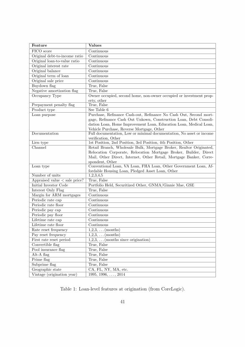
Feature Values

FICO score ContinuousOriginal debt-to-income ratio ContinuousOriginal loan-to-value ratio ContinuousOriginal interest rate ContinuousOriginal balance ContinuousOriginal term of loan ContinuousOriginal sale price ContinuousBuydown flag True, FalseNegative amortization flag True, FalseOccupancy Type Owner occupied, second home, non-owner occupied or investment prop-

erty, otherPrepayment penalty flag True, FalseProduct type See Table 6Loan purpose Purchase, Refinance Cash-out, Refinance No Cash Out, Second mort-

gage, Refinance Cash Out Unkown, Construction Loan, Debt Consoli-dation Loan, Home Improvement Loan, Education Loan, Medical Loan,Vehicle Purchase, Reverse Mortgage, Other

Documentation Full documentation, Low or minimal documentation, No asset or incomeverification, Other

Lien type 1st Position, 2nd Position, 3rd Position, 4th Position, OtherChannel Retail Branch, Wholesale Bulk, Mortgage Broker, Realtor Originated,

Relocation Corporate, Relocation Mortgage Broker, Builder, DirectMail, Other Direct, Internet, Other Retail, Mortgage Banker, Corre-spondent, Other

Loan type Conventional Loan, VA Loan, FHA Loan, Other Government Loan, Af-fordable Housing Loan, Pledged Asset Loan, Other

Number of units 1,2,3,4,5Appraised value < sale price? True, FalseInitial Investor Code Portfolio Held, Securitized Other, GNMA/Ginnie Mae, GSEInterest Only Flag True, FalseMargin for ARM mortgages ContinuousPeriodic rate cap ContinuousPeriodic rate floor ContinuousPeriodic pay cap ContinuousPeriodic pay floor ContinuousLifetime rate cap ContinuousLifetime rate floor ContinuousRate reset frequency 1,2,3, . . . (months)Pay reset frequency 1,2,3, . . . (months)First rate reset period 1,2,3, . . . (months since origination)Convertible flag True, FalsePool insurance flag True, FalseAlt-A flag True, FalsePrime flag True, FalseSubprime flag True, FalseGeographic state CA, FL, NY, MA, etc.Vintage (origination year) 1995, 1996, . . . , 2014

Table 1: Loan-level features at origination (from CoreLogic).

41

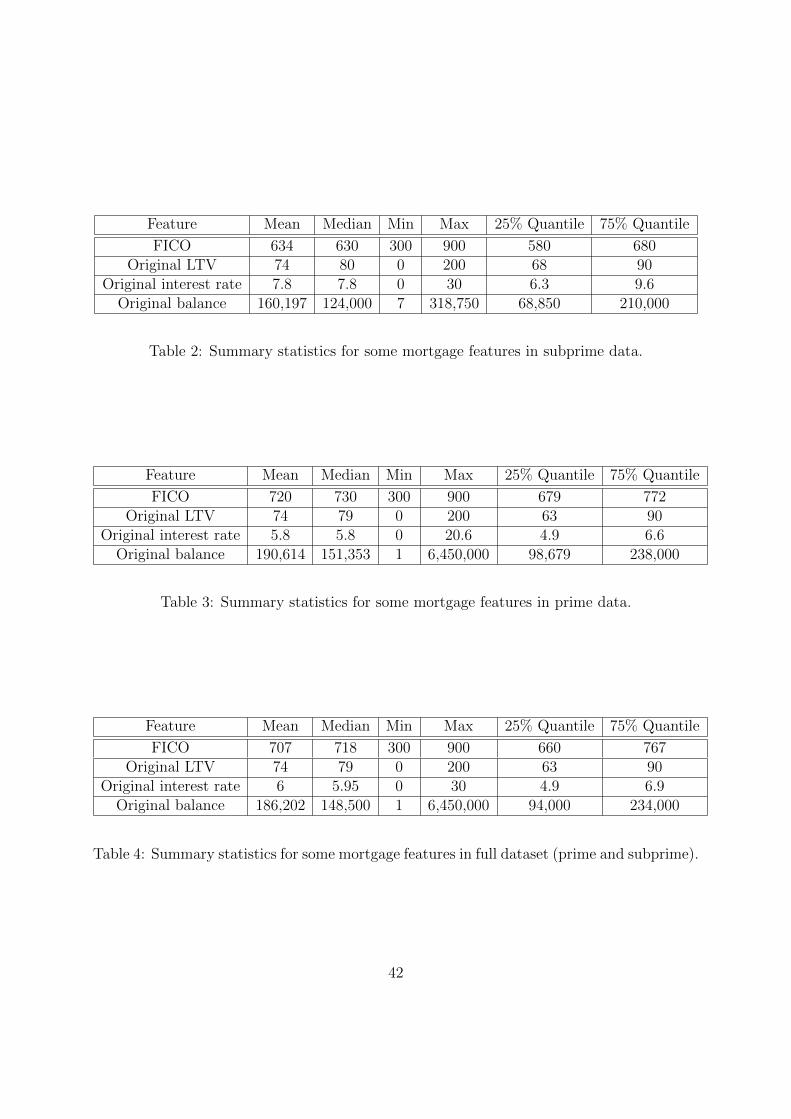
Feature Mean Median Min Max 25% Quantile 75% Quantile

FICO 634 630 300 900 580 680Original LTV 74 80 0 200 68 90

Original interest rate 7.8 7.8 0 30 6.3 9.6Original balance 160,197 124,000 7 318,750 68,850 210,000

Table 2: Summary statistics for some mortgage features in subprime data.

Feature Mean Median Min Max 25% Quantile 75% Quantile

FICO 720 730 300 900 679 772Original LTV 74 79 0 200 63 90

Original interest rate 5.8 5.8 0 20.6 4.9 6.6Original balance 190,614 151,353 1 6,450,000 98,679 238,000

Table 3: Summary statistics for some mortgage features in prime data.

Feature Mean Median Min Max 25% Quantile 75% Quantile

FICO 707 718 300 900 660 767Original LTV 74 79 0 200 63 90

Original interest rate 6 5.95 0 30 4.9 6.9Original balance 186,202 148,500 1 6,450,000 94,000 234,000

Table 4: Summary statistics for some mortgage features in full dataset (prime and subprime).

42

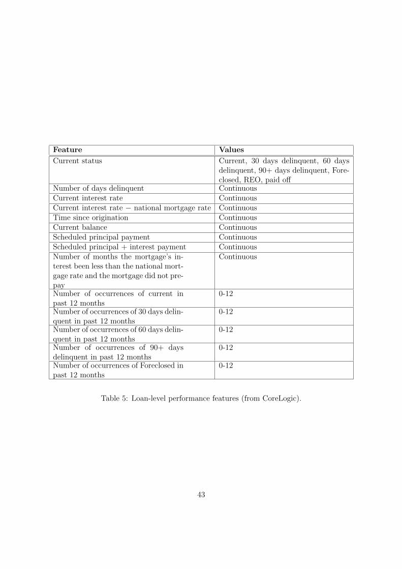
Feature Values

Current status Current, 30 days delinquent, 60 daysdelinquent, 90+ days delinquent, Fore-closed, REO, paid off

Number of days delinquent ContinuousCurrent interest rate ContinuousCurrent interest rate − national mortgage rate ContinuousTime since origination ContinuousCurrent balance ContinuousScheduled principal payment ContinuousScheduled principal + interest payment ContinuousNumber of months the mortgage’s in-terest been less than the national mort-gage rate and the mortgage did not pre-pay

Continuous

Number of occurrences of current inpast 12 months

0-12

Number of occurrences of 30 days delin-quent in past 12 months

0-12

Number of occurrences of 60 days delin-quent in past 12 months

0-12

Number of occurrences of 90+ daysdelinquent in past 12 months

0-12

Number of occurrences of Foreclosed inpast 12 months

0-12

Table 5: Loan-level performance features (from CoreLogic).

43

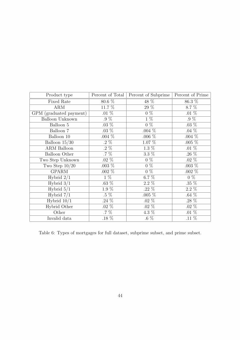
Product type Percent of Total Percent of Subprime Percent of Prime

Fixed Rate 80.6 % 48 % 86.3 %ARM 11.7 % 29 % 8.7 %

GPM (graduated payment) .01 % 0 % .01 %Balloon Unknown .9 % 1 % .9 %

Balloon 5 .03 % 0 % .03 %Balloon 7 .03 % .004 % .04 %Balloon 10 .004 % .006 % .004 %

Balloon 15/30 .2 % 1.07 % .005 %ARM Balloon .2 % 1.3 % .01 %Balloon Other .7 % 3.3 % .26 %

Two Step Unknown .02 % 0 % .02 %Two Step 10/20 .003 % 0 % .003 %

GPARM .002 % 0 % .002 %Hybrid 2/1 1 % 6.7 % 0 %Hybrid 3/1 .63 % 2.2 % .35 %Hybrid 5/1 1.9 % .22 % 2.2 %Hybrid 7/1 .5 % .005 % .64 %Hybrid 10/1 .24 % .02 % .28 %Hybrid Other .02 % .02 % .02 %

Other .7 % 4.3 % .01 %Invalid data .18 % .6 % .11 %

Table 6: Types of mortgages for full dataset, subprime subset, and prime subset.

44

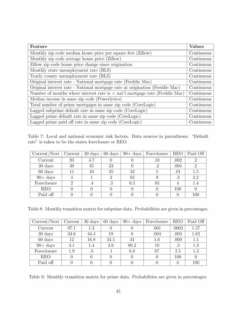
Feature Values

Monthly zip code median house price per square feet (Zillow) ContinuousMonthly zip code average house price (Zillow) ContinuousZillow zip code house price change since origination ContinuousMonthly state unemployment rate (BLS) ContinuousYearly county unemployment rate (BLS) ContinuousOriginal interest rate - National mortgage rate (Freddie Mac) ContinuousOriginal interest rate - National mortgage rate at origination (Freddie Mac) ContinuousNumber of months where interest rate is < nat’l mortgage rate (Freddie Mac) ContinuousMedian income in same zip code (Powerlytics) ContinuousTotal number of prime mortgages in same zip code (CoreLogic) ContinuousLagged subprime default rate in same zip code (CoreLogic) ContinuousLagged prime default rate in same zip code (CoreLogic) ContinuousLagged prime paid off rate in same zip code (CoreLogic) Continuous

Table 7: Local and national economic risk factors. Data sources in parentheses. “Defaultrate” is taken to be the states foreclosure or REO.

Current/Next Current 30 days 60 days 90+ days Foreclosure REO Paid Off

Current 93 4.7 0 0 .01 .002 230 days 30 45 23 0 .2 .004 260 days 11 16 35 32 5 .01 1.5

90+ days 4 1 2 82 9 .3 2.2Foreclosure 2 .4 .3 6.5 85 4 1.4

REO 0 0 0 0 0 100 0Paid off 0 0 0 0 0 0 100

Table 8: Monthly transition matrix for subprime data. Probabilities are given in percentages.

Current/Next Current 30 days 60 days 90+ days Foreclosure REO Paid Off

Current 97.1 1.3 0 0 .001 .0002 1.5730 days 34.6 44.4 19 0 .004 .003 1.8260 days 12 16.8 34.5 34 1.6 .009 1.1

90+ days 4.1 1.4 2.6 80.2 10 .3 1.3Foreclosure 1.9 .3 .1 6.8 87 2.5 1.3

REO 0 0 0 0 0 100 0Paid off 0 0 0 0 0 0 100

Table 9: Monthly transition matrix for prime data. Probabilities are given in percentages.

45

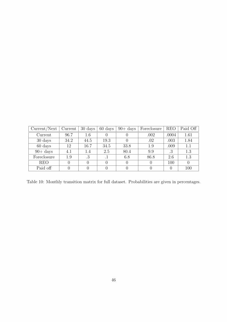
Current/Next Current 30 days 60 days 90+ days Foreclosure REO Paid Off

Current 96.7 1.6 0 0 .002 .0004 1.6130 days 34.2 44.5 19.3 0 .02 .003 1.8460 days 12 16.7 34.5 33.8 1.9 .009 1.1

90+ days 4.1 1.4 2.5 80.4 9.9 .3 1.3Foreclosure 1.9 .3 .1 6.8 86.8 2.6 1.3

REO 0 0 0 0 0 100 0Paid off 0 0 0 0 0 0 100

Table 10: Monthly transition matrix for full dataset. Probabilities are given in percentages.

46

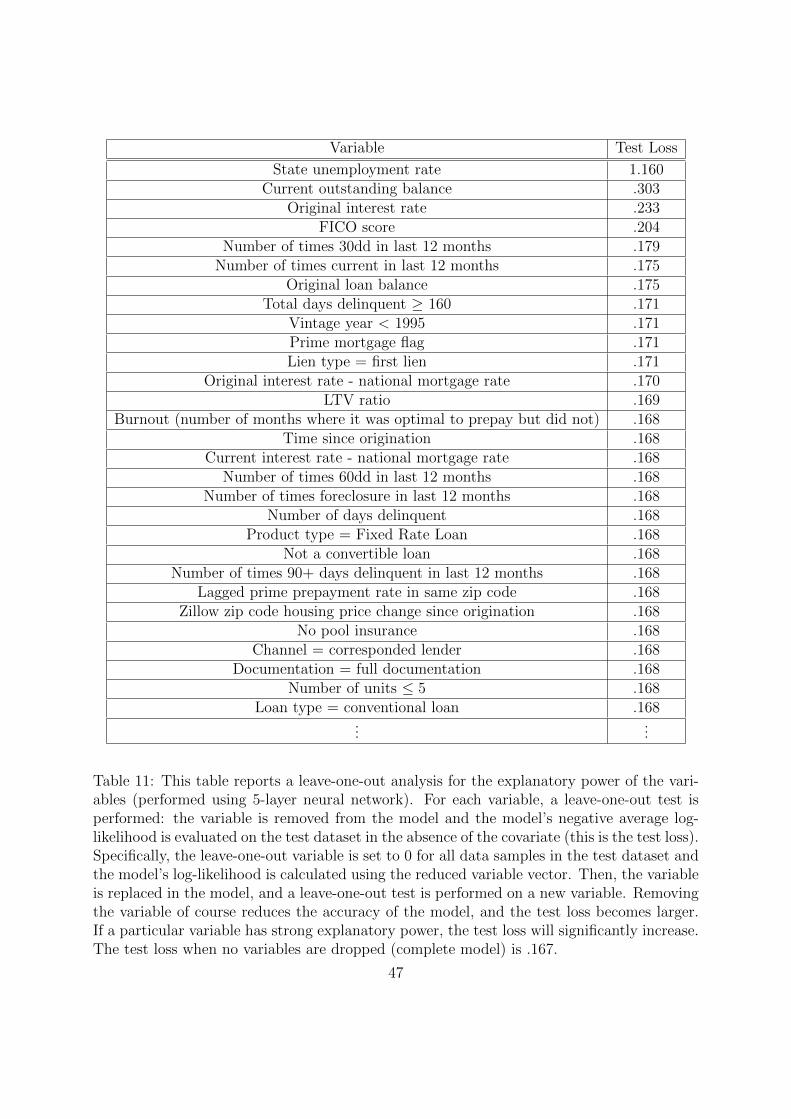
Variable Test Loss

State unemployment rate 1.160Current outstanding balance .303

Original interest rate .233FICO score .204

Number of times 30dd in last 12 months .179Number of times current in last 12 months .175

Original loan balance .175Total days delinquent ≥ 160 .171

Vintage year < 1995 .171Prime mortgage flag .171Lien type = first lien .171

Original interest rate - national mortgage rate .170LTV ratio .169

Burnout (number of months where it was optimal to prepay but did not) .168Time since origination .168

Current interest rate - national mortgage rate .168Number of times 60dd in last 12 months .168

Number of times foreclosure in last 12 months .168Number of days delinquent .168

Product type = Fixed Rate Loan .168Not a convertible loan .168

Number of times 90+ days delinquent in last 12 months .168Lagged prime prepayment rate in same zip code .168

Zillow zip code housing price change since origination .168No pool insurance .168

Channel = corresponded lender .168Documentation = full documentation .168

Number of units ≤ 5 .168Loan type = conventional loan .168

......

Table 11: This table reports a leave-one-out analysis for the explanatory power of the vari-ables (performed using 5-layer neural network). For each variable, a leave-one-out test isperformed: the variable is removed from the model and the model’s negative average log-likelihood is evaluated on the test dataset in the absence of the covariate (this is the test loss).Specifically, the leave-one-out variable is set to 0 for all data samples in the test dataset andthe model’s log-likelihood is calculated using the reduced variable vector. Then, the variableis replaced in the model, and a leave-one-out test is performed on a new variable. Removingthe variable of course reduces the accuracy of the model, and the test loss becomes larger.If a particular variable has strong explanatory power, the test loss will significantly increase.The test loss when no variables are dropped (complete model) is .167.

47

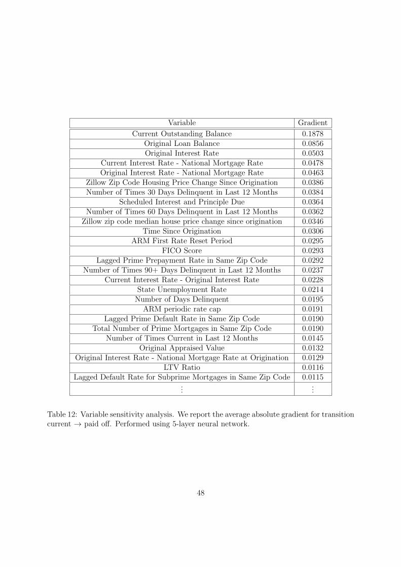
Variable Gradient

Current Outstanding Balance 0.1878Original Loan Balance 0.0856Original Interest Rate 0.0503

Current Interest Rate - National Mortgage Rate 0.0478Original Interest Rate - National Mortgage Rate 0.0463

Zillow Zip Code Housing Price Change Since Origination 0.0386Number of Times 30 Days Delinquent in Last 12 Months 0.0384

Scheduled Interest and Principle Due 0.0364Number of Times 60 Days Delinquent in Last 12 Months 0.0362

Zillow zip code median house price change since origination 0.0346Time Since Origination 0.0306

ARM First Rate Reset Period 0.0295FICO Score 0.0293

Lagged Prime Prepayment Rate in Same Zip Code 0.0292Number of Times 90+ Days Delinquent in Last 12 Months 0.0237

Current Interest Rate - Original Interest Rate 0.0228State Unemployment Rate 0.0214

Number of Days Delinquent 0.0195ARM periodic rate cap 0.0191

Lagged Prime Default Rate in Same Zip Code 0.0190Total Number of Prime Mortgages in Same Zip Code 0.0190

Number of Times Current in Last 12 Months 0.0145Original Appraised Value 0.0132

Original Interest Rate - National Mortgage Rate at Origination 0.0129LTV Ratio 0.0116

Lagged Default Rate for Subprime Mortgages in Same Zip Code 0.0115...

...

Table 12: Variable sensitivity analysis. We report the average absolute gradient for transitioncurrent → paid off. Performed using 5-layer neural network.

48

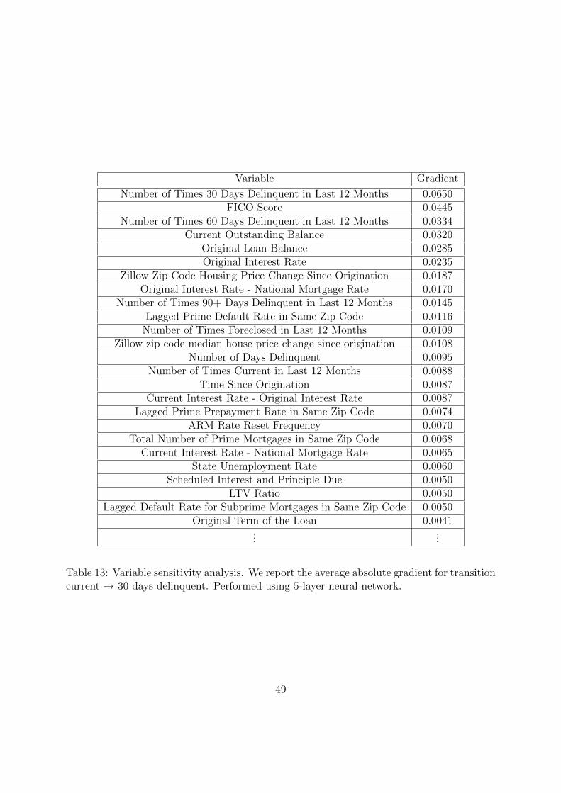
Variable Gradient

Number of Times 30 Days Delinquent in Last 12 Months 0.0650FICO Score 0.0445

Number of Times 60 Days Delinquent in Last 12 Months 0.0334Current Outstanding Balance 0.0320

Original Loan Balance 0.0285Original Interest Rate 0.0235

Zillow Zip Code Housing Price Change Since Origination 0.0187Original Interest Rate - National Mortgage Rate 0.0170

Number of Times 90+ Days Delinquent in Last 12 Months 0.0145Lagged Prime Default Rate in Same Zip Code 0.0116

Number of Times Foreclosed in Last 12 Months 0.0109Zillow zip code median house price change since origination 0.0108

Number of Days Delinquent 0.0095Number of Times Current in Last 12 Months 0.0088

Time Since Origination 0.0087Current Interest Rate - Original Interest Rate 0.0087

Lagged Prime Prepayment Rate in Same Zip Code 0.0074ARM Rate Reset Frequency 0.0070

Total Number of Prime Mortgages in Same Zip Code 0.0068Current Interest Rate - National Mortgage Rate 0.0065

State Unemployment Rate 0.0060Scheduled Interest and Principle Due 0.0050

LTV Ratio 0.0050Lagged Default Rate for Subprime Mortgages in Same Zip Code 0.0050

Original Term of the Loan 0.0041...

...

Table 13: Variable sensitivity analysis. We report the average absolute gradient for transitioncurrent → 30 days delinquent. Performed using 5-layer neural network.

49

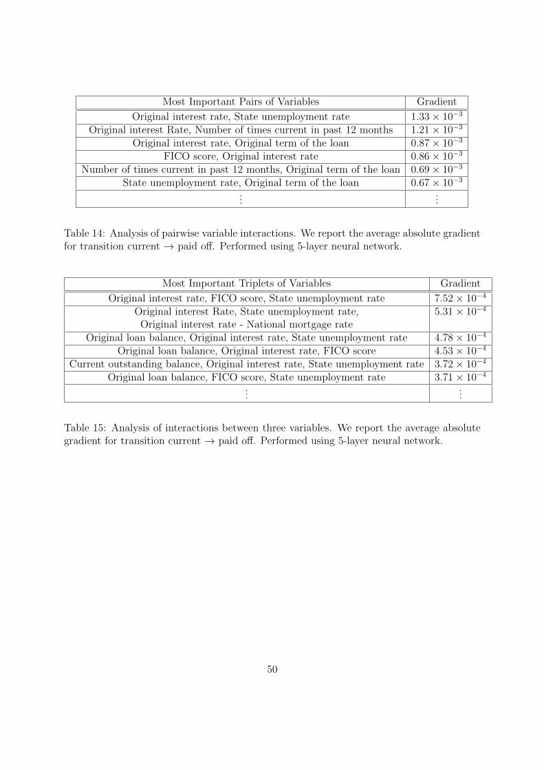
Most Important Pairs of Variables Gradient

Original interest rate, State unemployment rate 1.33× 10−3

Original interest Rate, Number of times current in past 12 months 1.21× 10−3

Original interest rate, Original term of the loan 0.87× 10−3

FICO score, Original interest rate 0.86× 10−3

Number of times current in past 12 months, Original term of the loan 0.69× 10−3

State unemployment rate, Original term of the loan 0.67× 10−3

......

Table 14: Analysis of pairwise variable interactions. We report the average absolute gradientfor transition current → paid off. Performed using 5-layer neural network.

Most Important Triplets of Variables Gradient

Original interest rate, FICO score, State unemployment rate 7.52× 10−4

Original interest Rate, State unemployment rate, 5.31× 10−4

Original interest rate - National mortgage rateOriginal loan balance, Original interest rate, State unemployment rate 4.78× 10−4

Original loan balance, Original interest rate, FICO score 4.53× 10−4

Current outstanding balance, Original interest rate, State unemployment rate 3.72× 10−4

Original loan balance, FICO score, State unemployment rate 3.71× 10−4

......

Table 15: Analysis of interactions between three variables. We report the average absolutegradient for transition current → paid off. Performed using 5-layer neural network.

50

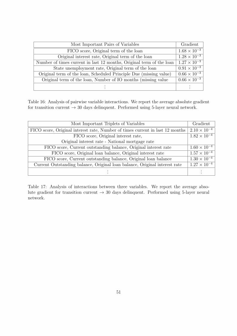
Most Important Pairs of Variables Gradient

FICO score, Original term of the loan 1.68× 10−3

Original interest rate, Original term of the loan 1.28× 10−3

Number of times current in last 12 months, Original term of the loan 1.27× 10−3

State unemployment rate, Original term of the loan 0.91× 10−3

Original term of the loan, Scheduled Principle Due (missing value) 0.66× 10−3

Original term of the loan, Number of IO months (missing value 0.66× 10−3

......

Table 16: Analysis of pairwise variable interactions. We report the average absolute gradientfor transition current → 30 days delinquent. Performed using 5-layer neural network.

Most Important Triplets of Variables Gradient

FICO score, Original interest rate, Number of times current in last 12 months 2.10× 10−4

FICO score, Original interest rate, 1.82× 10−4

Original interest rate - National mortgage rateFICO score, Current outstanding balance, Original interest rate 1.60× 10−4

FICO score, Original loan balance, Original interest rate 1.57× 10−4

FICO score, Current outstanding balance, Original loan balance 1.30× 10−4

Current Outstanding balance, Original loan balance, Original interest rate 1.27× 10−4

......

Table 17: Analysis of interactions between three variables. We report the average abso-lute gradient for transition current → 30 days delinquent. Performed using 5-layer neuralnetwork.

51

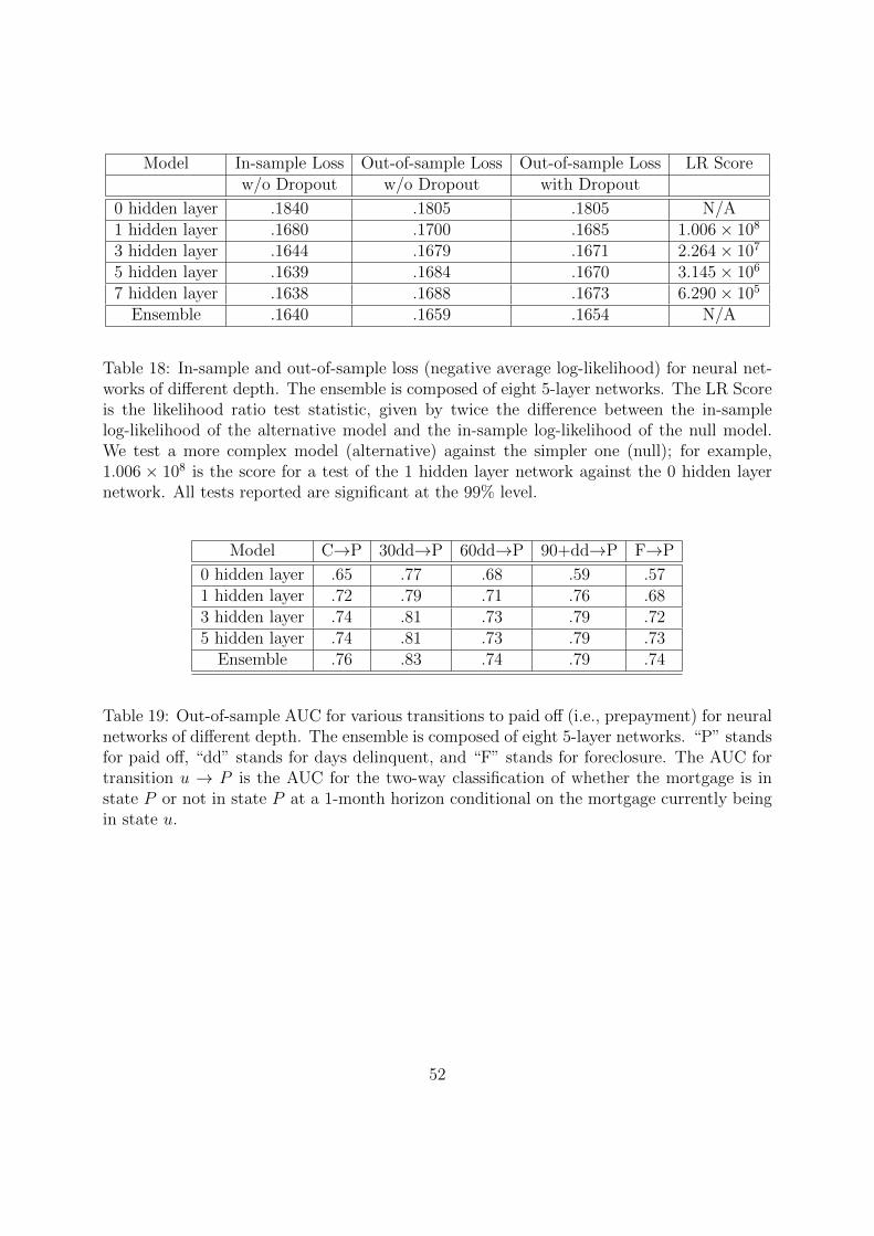
Model In-sample Loss Out-of-sample Loss Out-of-sample Loss LR Scorew/o Dropout w/o Dropout with Dropout

0 hidden layer .1840 .1805 .1805 N/A1 hidden layer .1680 .1700 .1685 1.006× 108

3 hidden layer .1644 .1679 .1671 2.264× 107

5 hidden layer .1639 .1684 .1670 3.145× 106

7 hidden layer .1638 .1688 .1673 6.290× 105

Ensemble .1640 .1659 .1654 N/A

Table 18: In-sample and out-of-sample loss (negative average log-likelihood) for neural net-works of different depth. The ensemble is composed of eight 5-layer networks. The LR Scoreis the likelihood ratio test statistic, given by twice the difference between the in-samplelog-likelihood of the alternative model and the in-sample log-likelihood of the null model.We test a more complex model (alternative) against the simpler one (null); for example,1.006 × 108 is the score for a test of the 1 hidden layer network against the 0 hidden layernetwork. All tests reported are significant at the 99% level.

Model C→P 30dd→P 60dd→P 90+dd→P F→P

0 hidden layer .65 .77 .68 .59 .571 hidden layer .72 .79 .71 .76 .683 hidden layer .74 .81 .73 .79 .725 hidden layer .74 .81 .73 .79 .73

Ensemble .76 .83 .74 .79 .74

Table 19: Out-of-sample AUC for various transitions to paid off (i.e., prepayment) for neuralnetworks of different depth. The ensemble is composed of eight 5-layer networks. “P” standsfor paid off, “dd” stands for days delinquent, and “F” stands for foreclosure. The AUC fortransition u → P is the AUC for the two-way classification of whether the mortgage is instate P or not in state P at a 1-month horizon conditional on the mortgage currently beingin state u.

52

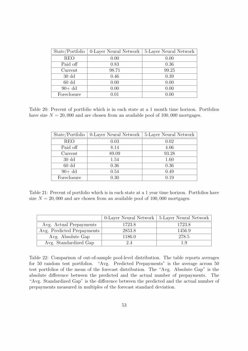
State/Portfolio 0-Layer Neural Network 5-Layer Neural Network

REO 0.00 0.00Paid off 0.83 0.36Current 98.71 99.2530 dd 0.46 0.3960 dd 0.00 0.00

90+ dd 0.00 0.00Foreclosure 0.01 0.00

Table 20: Percent of portfolio which is in each state at a 1 month time horizon. Portfolioshave size N = 20, 000 and are chosen from an available pool of 100, 000 mortgages.

State/Portfolio 0-Layer Neural Network 5-Layer Neural Network

REO 0.03 0.02Paid off 8.14 4.06Current 89.09 93.2830 dd 1.54 1.6060 dd 0.36 0.36

90+ dd 0.54 0.49Foreclosure 0.30 0.19

Table 21: Percent of portfolio which is in each state at a 1 year time horizon. Portfolios havesize N = 20, 000 and are chosen from an available pool of 100, 000 mortgages.

0-Layer Neural Network 5-Layer Neural Network

Avg. Actual Prepayments 1723.8 1723.8Avg. Predicted Prepayments 2853.8 1456.9

Avg. Absolute Gap 1186.0 278.5Avg. Standardized Gap 2.4 1.9

Table 22: Comparison of out-of-sample pool-level distribution. The table reports averagesfor 50 random test portfolios. “Avg. Predicted Prepayments” is the average across 50test portfolios of the mean of the forecast distribution. The “Avg. Absolute Gap” is theabsolute difference between the predicted and the actual number of prepayments. The“Avg. Standardized Gap” is the difference between the predicted and the actual number ofprepayments measured in multiples of the forecast standard deviation.

53

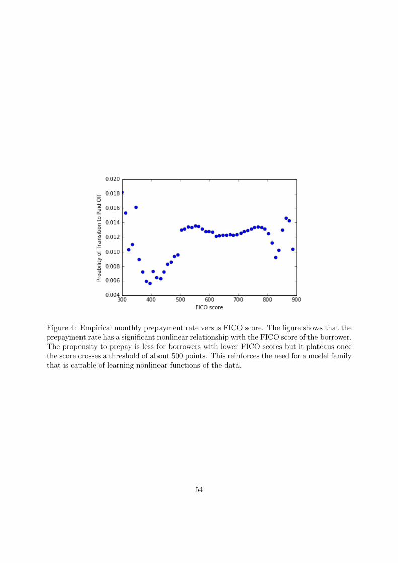
Figure 4: Empirical monthly prepayment rate versus FICO score. The figure shows that theprepayment rate has a significant nonlinear relationship with the FICO score of the borrower.The propensity to prepay is less for borrowers with lower FICO scores but it plateaus oncethe score crosses a threshold of about 500 points. This reinforces the need for a model familythat is capable of learning nonlinear functions of the data.

54

Figure 5: Empirical monthly prepayment rate versus time since origination (loan age). Thefigure shows that the prepayment rate has a significant nonlinear relationship with the ageof the mortgage. Several spikes in the rate occur at 1, 2, and 3 years. These might be dueto the expiration of prepayment penalties or ARM and hybrid mortgages having rate resets.Many of the subprime mortgages started with low teaser rates and would later jump tohigher rates; borrowers would refinance to avoid these rate jumps.

55

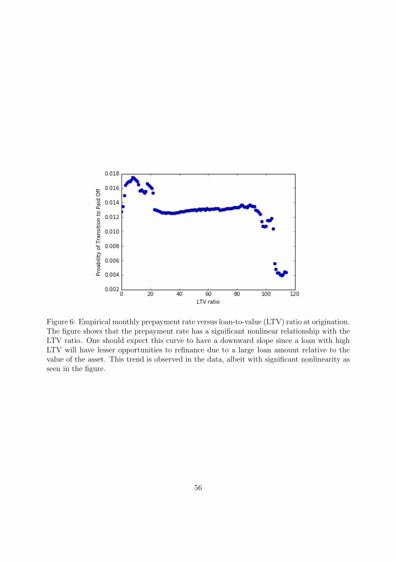
Figure 6: Empirical monthly prepayment rate versus loan-to-value (LTV) ratio at origination.The figure shows that the prepayment rate has a significant nonlinear relationship with theLTV ratio. One should expect this curve to have a downward slope since a loan with highLTV will have lesser opportunities to refinance due to a large loan amount relative to thevalue of the asset. This trend is observed in the data, albeit with significant nonlinearity asseen in the figure.

56

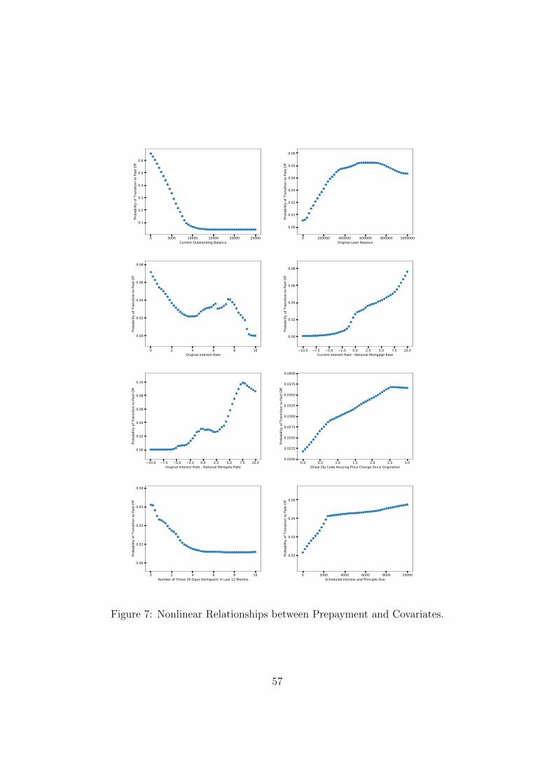
0 5000 10000 15000 20000 25000Current Outstanding Balance

0.1

0.2

0.3

0.4

0.5

0.6

Prob

abilit

y of

Tra

nsiti

on to

Pai

d Of

f

0 200000 400000 600000 800000 1000000Original Loan Balance

0.00

0.01

0.02

0.03

0.04

0.05

0.06

Prob

abilit

y of

Tra

nsiti

on to

Pai

d Of

f

0 2 4 6 8 10Original Interest Rate

0.00

0.02

0.04

0.06

0.08

Prob

abilit

y of

Tra

nsiti

on to

Pai

d Of

f

10.0 7.5 5.0 2.5 0.0 2.5 5.0 7.5 10.0Current Interest Rate - National Mortgage Rate

0.00

0.02

0.04

0.06

0.08

Prob

abilit

y of

Tra

nsiti

on to

Pai

d Of

f

10.0 7.5 5.0 2.5 0.0 2.5 5.0 7.5 10.0Original Interest Rate - National Mortgate Rate

0.00

0.02

0.04

0.06

0.08

0.10

Prob

abilit

y of

Tra

nsiti

on to

Pai

d Of

f

0.0 0.5 1.0 1.5 2.0 2.5 3.0Zillow Zip Code Housing Price Change Since Origination

0.0200

0.0225

0.0250

0.0275

0.0300

0.0325

0.0350

0.0375

0.0400

Prob

abilit

y of

Tra

nsiti

on to

Pai

d Of

f

0 2 4 6 8 10Number of Times 30 Days Delinquent in Last 12 Months

0.00

0.01

0.02

0.03

0.04

Prob

abilit

y of

Tra

nsiti

on to

Pai

d Of

f

0 2000 4000 6000 8000 10000Scheduled Interest and Principle Due

0.02

0.03

0.04

0.05

Prob

abilit

y of

Tra

nsiti

on to

Pai

d Of

f

Figure 7: Nonlinear Relationships between Prepayment and Covariates.

57

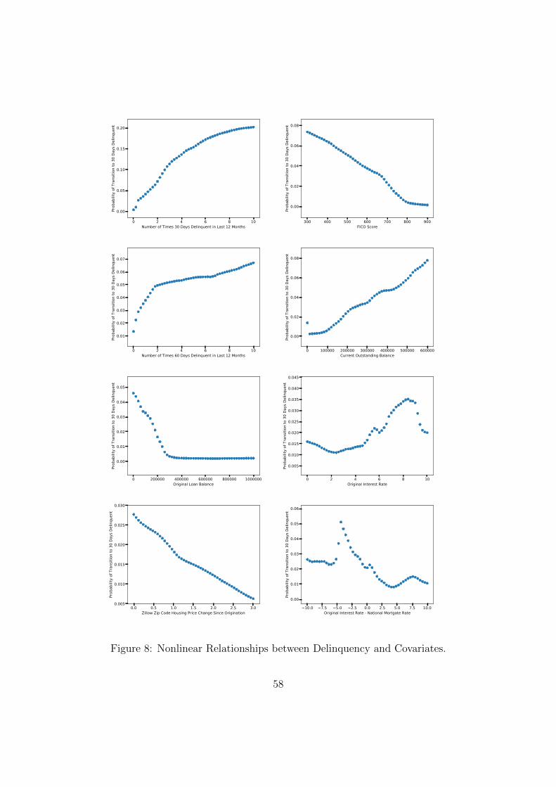
0 2 4 6 8 10Number of Times 30 Days Delinquent in Last 12 Months

0.00

0.05

0.10

0.15

0.20

Prob

abilit

y of

Tra

nsiti

on to

30

Days

Del

inqu

ent

300 400 500 600 700 800 900FICO Score

0.00

0.02

0.04

0.06

0.08

Prob

abilit

y of

Tra

nsiti

on to

30

Days

Del

inqu

ent

0 2 4 6 8 10Number of Times 60 Days Delinquent in Last 12 Months

0.01

0.02

0.03

0.04

0.05

0.06

0.07

Prob

abilit

y of

Tra

nsiti

on to

30

Days

Del

inqu

ent

0 100000 200000 300000 400000 500000 600000Current Outstanding Balance

0.00

0.02

0.04

0.06

0.08

Prob

abilit

y of

Tra

nsiti

on to

30

Days

Del

inqu

ent

0 200000 400000 600000 800000 1000000Original Loan Balance

0.00

0.01

0.02

0.03

0.04

0.05

Prob

abilit

y of

Tra

nsiti

on to

30

Days

Del

inqu

ent

0 2 4 6 8 10Original Interest Rate

0.005

0.010

0.015

0.020

0.025

0.030

0.035

0.040

0.045

Prob

abilit

y of

Tra

nsiti

on to

30

Days

Del

inqu

ent

0.0 0.5 1.0 1.5 2.0 2.5 3.0Zillow Zip Code Housing Price Change Since Origination

0.005

0.010

0.015

0.020

0.025

0.030

Prob

abilit

y of

Tra

nsiti

on to

30

Days

Del

inqu

ent

10.0 7.5 5.0 2.5 0.0 2.5 5.0 7.5 10.0Original Interest Rate - National Mortgate Rate

0.00

0.01

0.02

0.03

0.04

0.05

0.06

Prob

abilit

y of

Tra

nsiti

on to

30

Days

Del

inqu

ent

Figure 8: Nonlinear Relationships between Delinquency and Covariates.

58

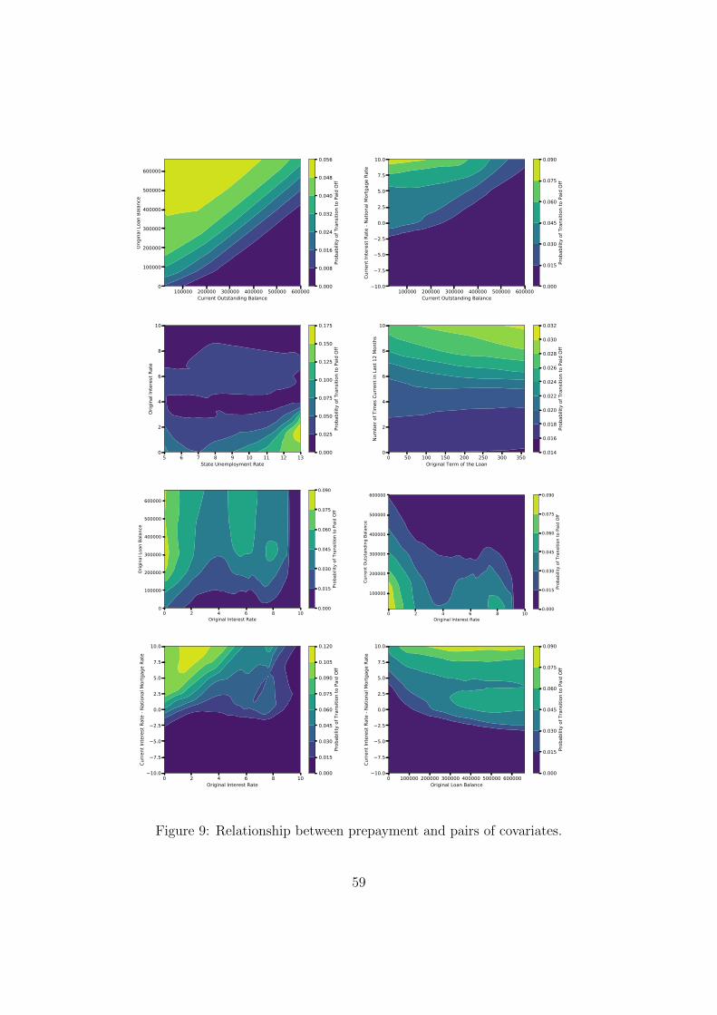
100000 200000 300000 400000 500000 600000Current Outstanding Balance

0

100000

200000

300000

400000

500000

600000

Orig

inal

Loa

n Ba

lanc

e

0.000

0.008

0.016

0.024

0.032

0.040

0.048

0.056

Prob

abilit

y of

Tra

nsiti

on to

Pai

d Of

f

100000 200000 300000 400000 500000 600000Current Outstanding Balance

10.0

7.5

5.0

2.5

0.0

2.5

5.0

7.5

10.0

Curre

nt In

tere

st R

ate

- Nat

iona

l Mor

tgag

e Ra

te

0.000

0.015

0.030

0.045

0.060

0.075

0.090

Prob

abilit

y of

Tra

nsiti

on to

Pai

d Of

f

5 6 7 8 9 10 11 12 13State Unemployment Rate

0

2

4

6

8

10

Orig

inal

Inte

rest

Rat

e

0.000

0.025

0.050

0.075

0.100

0.125

0.150

0.175Pr

obab

ility

of T

rans

ition

to P

aid

Off

0 50 100 150 200 250 300 350Original Term of the Loan

0

2

4

6

8

10

Num

ber o

f Tim

es C

urre

nt in

Las

t 12

Mon

ths

0.014

0.016

0.018

0.020

0.022

0.024

0.026

0.028

0.030

0.032

Prob

abilit

y of

Tra

nsiti

on to

Pai

d Of

f

0 2 4 6 8 10Original Interest Rate

0

100000

200000

300000

400000

500000

600000

Orig

inal

Loa

n Ba

lanc

e

0.000

0.015

0.030

0.045

0.060

0.075

0.090

Prob

abilit

y of

Tra

nsiti

on to

Pai

d Of

f

0 2 4 6 8 10Original Interest Rate

100000

200000

300000

400000

500000

600000

Curre

nt O

utst

andi

ng B

alan

ce

0.000

0.015

0.030

0.045

0.060

0.075

0.090

Prob

abilit

y of

Tra

nsiti

on to

Pai

d Of

f

0 2 4 6 8 10Original Interest Rate

10.0

7.5

5.0

2.5

0.0

2.5

5.0

7.5

10.0

Curre

nt In

tere

st R

ate

- Nat

iona

l Mor

tgag

e Ra

te

0.000

0.015

0.030

0.045

0.060

0.075

0.090

0.105

0.120

Prob

abilit

y of

Tra

nsiti

on to

Pai

d Of

f

0 100000 200000 300000 400000 500000 600000Original Loan Balance

10.0

7.5

5.0

2.5

0.0

2.5

5.0

7.5

10.0

Curre

nt In

tere

st R

ate

- Nat

iona

l Mor

tgag

e Ra

te

0.000

0.015

0.030

0.045

0.060

0.075

0.090

Prob

abilit

y of

Tra

nsiti

on to

Pai

d Of

f

Figure 9: Relationship between prepayment and pairs of covariates.

59

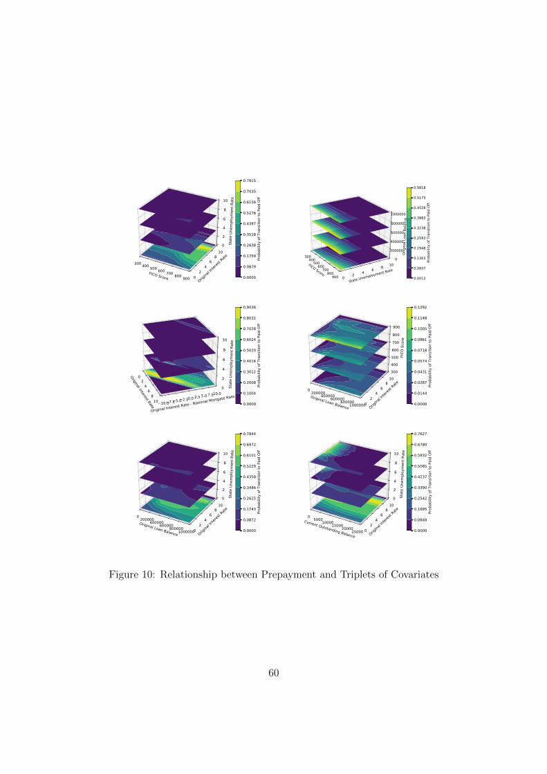
FICO Score

300 400 500 600 700 800 900 Origina

l Inter

est Rate

02

46

810

Stat

e Un

empl

oym

ent R

ate

0

2

4

6

8

10

0.0000

0.0879

0.1759

0.2638

0.3518

0.4397

0.5276

0.6156

0.7035

0.7915

Prob

abilit

y of

Tra

nsiti

on to

Pai

d Of

fFICO Score

300400

500600

700800

900State Unemployment Rate

0 2 4 6 8 10

Orig

inal

Loa

n Ba

lanc

e

0

200000

400000

600000

800000

1000000

0.0012

0.0657

0.1303

0.1948

0.2593

0.3238

0.3883

0.4528

0.5173

0.5818

Prob

abilit

y of

Tra

nsiti

on to

Pai

d Of

f

Original Interest Rate

02

46

810

Original Interest Rate - National Mortgate Rate10.07.5 5.0 2.50.0 2.5 5.0 7.510.0

Stat

e Un

empl

oym

ent R

ate

0

2

4

6

8

10

0.0000

0.1004

0.2008

0.3012

0.4016

0.5020

0.6024

0.7028

0.8032

0.9036

Prob

abilit

y of

Tra

nsiti

on to

Pai

d Of

f

Original Loan Balance

0 2000004000006000008000001000000 Orig

inal In

terest

Rate

02

46

810

FICO

Sco

re

300400500600700800

900

0.0000

0.0144

0.0287

0.0431

0.0574

0.0718

0.0861

0.1005

0.1148

0.1292

Prob

abilit

y of

Tra

nsiti

on to

Pai

d Of

f

Original Loan Balance

0 2000004000006000008000001000000 Orig

inal In

terest

Rate

02

46

810

Stat

e Un

empl

oym

ent R

ate

0

2

4

6

8

10

0.0000

0.0872

0.1743

0.2615

0.3486

0.4358

0.5229

0.6101

0.6972

0.7844

Prob

abilit

y of

Tra

nsiti

on to

Pai

d Of

f

Current Outstanding Balance

0 500010000150002000025000 Orig

inal In

terest

Rate

02

46

810

Stat

e Un

empl

oym

ent R

ate

0

2

4

6

8

10

0.0000

0.0848

0.1695

0.2542

0.3390

0.4237

0.5085

0.5932

0.6780

0.7627Pr

obab

ility

of T

rans

ition

to P

aid

Off

Figure 10: Relationship between Prepayment and Triplets of Covariates

60

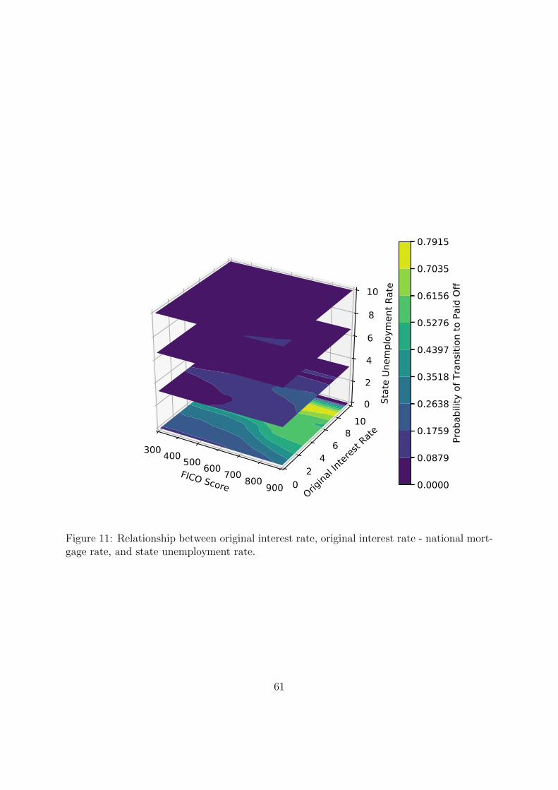
FICO Score

300 400 500 600 700 800 900 Origina

l Inter

est Rate

02

46

810

Stat

e Un

empl

oym

ent R

ate

0

2

4

6

8

10

0.0000

0.0879

0.1759

0.2638

0.3518

0.4397

0.5276

0.6156

0.7035

0.7915

Prob

abilit

y of

Tra

nsiti

on to

Pai

d Of

f

Figure 11: Relationship between original interest rate, original interest rate - national mort-gage rate, and state unemployment rate.

61

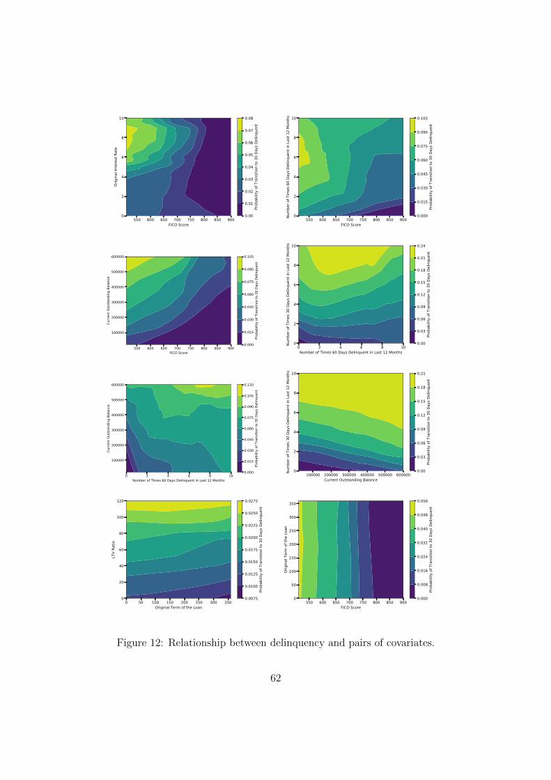
550 600 650 700 750 800 850 900FICO Score

0

2

4

6

8

10Or

igin

al In

tere

st R

ate

0.00

0.01

0.02

0.03

0.04

0.05

0.06

0.07

0.08

Prob

abilit

y of

Tra

nsiti

on to

30

Days

Del

inqu

ent

550 600 650 700 750 800 850 900FICO Score

0

2

4

6

8

10

Num

ber o

f Tim

es 6

0 Da

ys D

elin

quen

t in

Last

12

Mon

ths

0.000

0.015

0.030

0.045

0.060

0.075

0.090

0.105

Prob

abilit

y of

Tra

nsiti

on to

30

Days

Del

inqu

ent

550 600 650 700 750 800 850 900FICO Score

100000

200000

300000

400000

500000

600000

Curre

nt O

utst

andi

ng B

alan

ce

0.000

0.015

0.030

0.045

0.060

0.075

0.090

0.105Pr

obab

ility

of T

rans

ition

to 3

0 Da

ys D

elin

quen

t

0 2 4 6 8 10Number of Times 60 Days Delinquent in Last 12 Months

0

2

4

6

8

10

Num

ber o

f Tim

es 3

0 Da

ys D

elin

quen

t in

Last

12

Mon

ths

0.00

0.03

0.06

0.09

0.12

0.15

0.18

0.21

0.24

Prob

abilit

y of

Tra

nsiti

on to

30

Days

Del

inqu

ent

0 2 4 6 8 10Number of Times 60 Days Delinquent in Last 12 Months

100000

200000

300000

400000

500000

600000

Curre

nt O

utst

andi

ng B

alan

ce

0.000

0.015

0.030

0.045

0.060

0.075

0.090

0.105

0.120

Prob

abilit

y of

Tra

nsiti

on to

30

Days

Del

inqu

ent

100000 200000 300000 400000 500000 600000Current Outstanding Balance

0

2

4

6

8

10

Num

ber o

f Tim

es 3

0 Da

ys D

elin

quen

t in

Last

12

Mon

ths

0.00

0.03

0.06

0.09

0.12

0.15

0.18

0.21

Prob

abilit

y of

Tra

nsiti

on to

30

Days

Del

inqu

ent

0 50 100 150 200 250 300 350Original Term of the Loan

0

20

40

60

80

100

120

LTV

Ratio

0.0075

0.0100

0.0125

0.0150

0.0175

0.0200

0.0225

0.0250

0.0275

Prob

abilit

y of

Tra

nsiti

on to

30

Days

Del

inqu

ent

550 600 650 700 750 800 850 900FICO Score

0

50

100

150

200

250

300

350

Orig

inal

Ter

m o

f the

Loa

n

0.000

0.008

0.016

0.024

0.032

0.040

0.048

0.056

Prob

abilit

y of

Tra

nsiti

on to

30

Days

Del

inqu

ent

Figure 12: Relationship between delinquency and pairs of covariates.

62

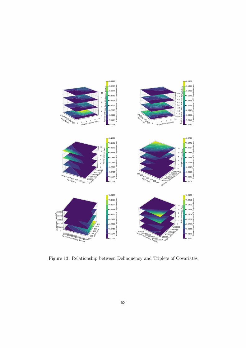
FICO Score

300400500600700800900Original Interest Rate

0 2 4 6 8 10

Num

ber o

f Tim

es C

urre

nt in

Las

t 12

Mon

ths

0

2

4

6

8

10

0.0015

0.0337

0.0660

0.0983

0.1306

0.1629

0.1952

0.2274

0.2597

0.2920

Prob

abilit

y of

Tra

nsiti

on to

30

Days

Del

inqu

ent

FICO Score

300400500600700

800900

Original Interest Rate0 2 4 6 8 10

Orig

inal

Inte

rest

Rat

e - N

atio

nal M

ortg

ate

Rate

10.07.55.02.5

0.02.55.07.510.0

0.0012

0.0189

0.0366

0.0543

0.0721

0.0898

0.1075

0.1252

0.1429

0.1607

Prob

abilit

y of

Tra

nsiti

on to

30

Days

Del

inqu

ent

FICO Score

300 400 500 600 700 800 900 Origina

l Loan

Balance

0200000

400000600000

8000001000000

Orig

inal

Inte

rest

Rat

e

0

2

4

6

8

10

0.0006

0.0204

0.0402

0.0600

0.0799

0.0997

0.1195

0.1393

0.1592

0.1790

Prob

abilit

y of

Tra

nsiti

on to

30

Days

Del

inqu

ent

FICO Score

300400

500600

700800

900Current O

utstanding Balance

100000200000

300000400000

500000600000

Orig

inal

Inte

rest

Rat

e

0

2

4

6

8

10

0.0006

0.0310

0.0615

0.0919

0.1224

0.1528

0.1833

0.2137

0.2442

0.2746

Prob

abilit

y of

Tra

nsiti

on to

30

Days

Del

inqu

ent

FICO

Scor

e

300400

500600

700800

900Current Outstanding Balance

100000200000300000400000500000600000

Original Loan Balance

0

200000

400000

600000

800000

1000000

0.0005

0.0244

0.0483

0.0722

0.0961

0.1200

0.1438

0.1677

0.1916

0.2155

Prob

abilit

y of

Tra

nsiti

on to

30

Days

Del

inqu

ent

Current Outstanding Balance

100000200000

300000400000

500000600000 Orig

inal Loan

Balance

0200000

400000600000

8000001000000

Orig

inal

Inte

rest

Rat

e

0

2

4

6

8

10

0.0020

0.0278

0.0535

0.0793

0.1051

0.1308

0.1566

0.1823

0.2081

0.2338Pr

obab

ility

of T

rans

ition

to 3

0 Da

ys D

elin

quen

t

Figure 13: Relationship between Delinquency and Triplets of Covariates

63

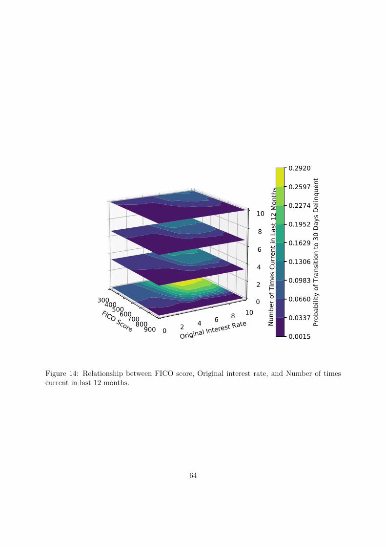
FICO Score

300400500600700800900Original Interest Rate

0 2 4 6 8 10

Num

ber o

f Tim

es C

urre

nt in

Las

t 12

Mon

ths

0

2

4

6

8

10

0.0015

0.0337

0.0660

0.0983

0.1306

0.1629

0.1952

0.2274

0.2597

0.2920

Prob

abilit

y of

Tra

nsiti

on to

30

Days

Del

inqu

ent

Figure 14: Relationship between FICO score, Original interest rate, and Number of timescurrent in last 12 months.

64

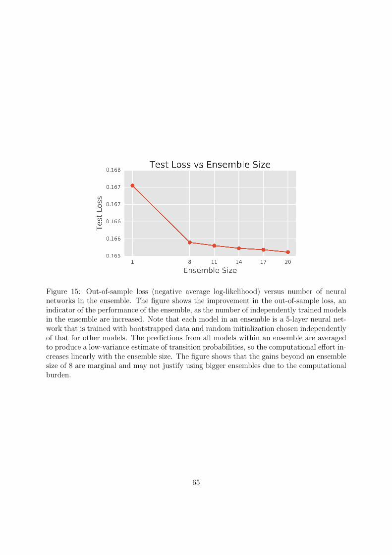
Figure 15: Out-of-sample loss (negative average log-likelihood) versus number of neuralnetworks in the ensemble. The figure shows the improvement in the out-of-sample loss, anindicator of the performance of the ensemble, as the number of independently trained modelsin the ensemble are increased. Note that each model in an ensemble is a 5-layer neural net-work that is trained with bootstrapped data and random initialization chosen independentlyof that for other models. The predictions from all models within an ensemble are averagedto produce a low-variance estimate of transition probabilities, so the computational effort in-creases linearly with the ensemble size. The figure shows that the gains beyond an ensemblesize of 8 are marginal and may not justify using bigger ensembles due to the computationalburden.

65

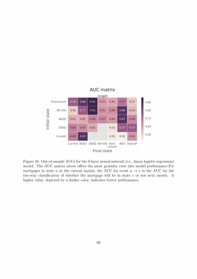
Figure 16: Out-of-sample AUCs for the 0-layer neural network (i.e., linear logistic regression)model. The AUC matrix above offers the most granular view into model performance.Formortgages in state u in the current month, the AUC for event u → v is the AUC for thetwo-way classification of whether the mortgage will be in state v or not next month. Ahigher value, depicted by a darker color, indicates better performance.

66

Figure 17: Out-of-sample AUCs for the 1-layer neural network. The AUC matrix above offersthe most granular view into model performance. For mortgages in state u in the currentmonth, the AUC for event u → v is the AUC for the two-way classification of whether themortgage will be in state v or not next month. A higher value, depicted by a darker color,indicates better performance. We see marked improvement in the AUC values in going fromthe 0-layer model to the 1-layer network, especially for transitions to foreclosure and paidoff as well as for the transitions from the delinquent states to current.

67

Figure 18: Out-of-sample AUCs for the 3-layer neural network. The AUC matrix above offersthe most granular view into model performance. For mortgages in state u in the currentmonth, the AUC for event u → v is the AUC for the two-way classification of whether themortgage will be in state v or not next month. A higher value, depicted by a darker color,indicates better performance. We see further improvement in the AUC values in going fromthe shallow networks to the deeper networks.

68

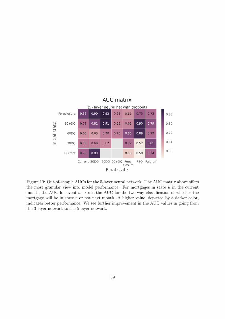
Figure 19: Out-of-sample AUCs for the 5-layer neural network. The AUC matrix above offersthe most granular view into model performance. For mortgages in state u in the currentmonth, the AUC for event u → v is the AUC for the two-way classification of whether themortgage will be in state v or not next month. A higher value, depicted by a darker color,indicates better performance. We see further improvement in the AUC values in going fromthe 3-layer network to the 5-layer network.

69

Figure 20: Out-of-sample AUCs for an ensemble of independently trained 5-layer neuralnetworks. The AUC matrix above offers the most granular view into model performance.For mortgages in state u in the current month, the AUC for event u → v is the AUC forthe two-way classification of whether the mortgage will be in state v or not next month. Ahigher value, depicted by a darker color, indicates better performance. In going from the5-layer neural network to their ensemble, every transition in the matrix sees an improvementin prediction.

70

Figure 21: Out-of-sample ROC curves for various models for the transition current → paidoff. The ROC curve corresponding to the ensemble dominates the curves for the individualnetworks, which in turn dominate the curve for the 0-layer (logistic regression) model. Thisimplies that for those mortgages that are presently in the current state, predicting whetherthe state next month would be paid off or not is best predicted by the ensemble, followedby the networks with at least one layer, and then by the 0-layer model. Further, the gapbetween the curves for the 0-layer model and those for the deep neural networks indicatesthe significant gain in predictive power due to the modeling of more complex nonlinearrelationships obtained by adding multiple hidden layers to the model.

71

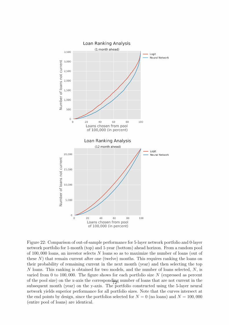
Figure 22: Comparison of out-of-sample performance for 5-layer network portfolio and 0-layernetwork portfolio for 1-month (top) and 1-year (bottom) ahead horizon. From a random poolof 100, 000 loans, an investor selects N loans so as to maximize the number of loans (out ofthese N) that remain current after one (twelve) months. This requires ranking the loans ontheir probability of remaining current in the next month (year) and then selecting the topN loans. This ranking is obtained for two models, and the number of loans selected, N , isvaried from 0 to 100, 000. The figure shows for each portfolio size N (expressed as percentof the pool size) on the x-axis the corresponding number of loans that are not current in thesubsequent month (year) on the y-axis. The portfolio constructed using the 5-layer neuralnetwork yields superior performance for all portfolio sizes. Note that the curves intersect atthe end points by design, since the portfolios selected for N = 0 (no loans) and N = 100, 000(entire pool of loans) are identical.

72

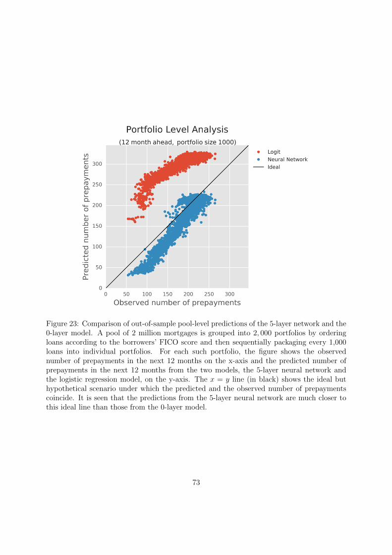
Figure 23: Comparison of out-of-sample pool-level predictions of the 5-layer network and the0-layer model. A pool of 2 million mortgages is grouped into 2, 000 portfolios by orderingloans according to the borrowers’ FICO score and then sequentially packaging every 1,000loans into individual portfolios. For each such portfolio, the figure shows the observednumber of prepayments in the next 12 months on the x-axis and the predicted number ofprepayments in the next 12 months from the two models, the 5-layer neural network andthe logistic regression model, on the y-axis. The x = y line (in black) shows the ideal buthypothetical scenario under which the predicted and the observed number of prepaymentscoincide. It is seen that the predictions from the 5-layer neural network are much closer tothis ideal line than those from the 0-layer model.

73

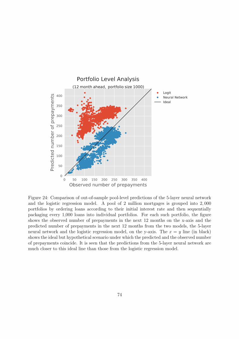
Figure 24: Comparison of out-of-sample pool-level predictions of the 5-layer neural networkand the logistic regression model. A pool of 2 million mortgages is grouped into 2, 000portfolios by ordering loans according to their initial interest rate and then sequentiallypackaging every 1,000 loans into individual portfolios. For each such portfolio, the figureshows the observed number of prepayments in the next 12 months on the x-axis and thepredicted number of prepayments in the next 12 months from the two models, the 5-layerneural network and the logistic regression model, on the y-axis. The x = y line (in black)shows the ideal but hypothetical scenario under which the predicted and the observed numberof prepayments coincide. It is seen that the predictions from the 5-layer neural network aremuch closer to this ideal line than those from the logistic regression model.

74

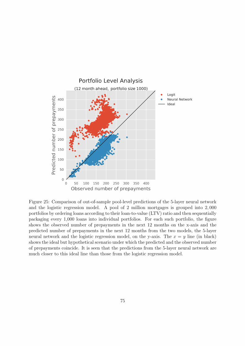
Figure 25: Comparison of out-of-sample pool-level predictions of the 5-layer neural networkand the logistic regression model. A pool of 2 million mortgages is grouped into 2, 000portfolios by ordering loans according to their loan-to-value (LTV) ratio and then sequentiallypackaging every 1,000 loans into individual portfolios. For each such portfolio, the figureshows the observed number of prepayments in the next 12 months on the x-axis and thepredicted number of prepayments in the next 12 months from the two models, the 5-layerneural network and the logistic regression model, on the y-axis. The x = y line (in black)shows the ideal but hypothetical scenario under which the predicted and the observed numberof prepayments coincide. It is seen that the predictions from the 5-layer neural network aremuch closer to this ideal line than those from the logistic regression model.

75

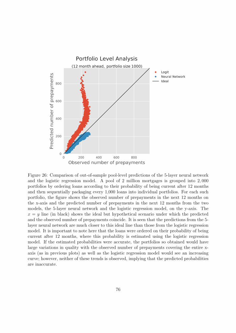
Figure 26: Comparison of out-of-sample pool-level predictions of the 5-layer neural networkand the logistic regression model. A pool of 2 million mortgages is grouped into 2, 000portfolios by ordering loans according to their probability of being current after 12 monthsand then sequentially packaging every 1,000 loans into individual portfolios. For each suchportfolio, the figure shows the observed number of prepayments in the next 12 months onthe x-axis and the predicted number of prepayments in the next 12 months from the twomodels, the 5-layer neural network and the logistic regression model, on the y-axis. Thex = y line (in black) shows the ideal but hypothetical scenario under which the predictedand the observed number of prepayments coincide. It is seen that the predictions from the 5-layer neural network are much closer to this ideal line than those from the logistic regressionmodel. It is important to note here that the loans were ordered on their probability of beingcurrent after 12 months, where this probability is estimated using the logistic regressionmodel. If the estimated probabilities were accurate, the portfolios so obtained would havelarge variations in quality with the observed number of prepayments covering the entire x-axis (as in previous plots) as well as the logistic regression model would see an increasingcurve; however, neither of these trends is observed, implying that the predicted probabilitiesare inaccurate.

76

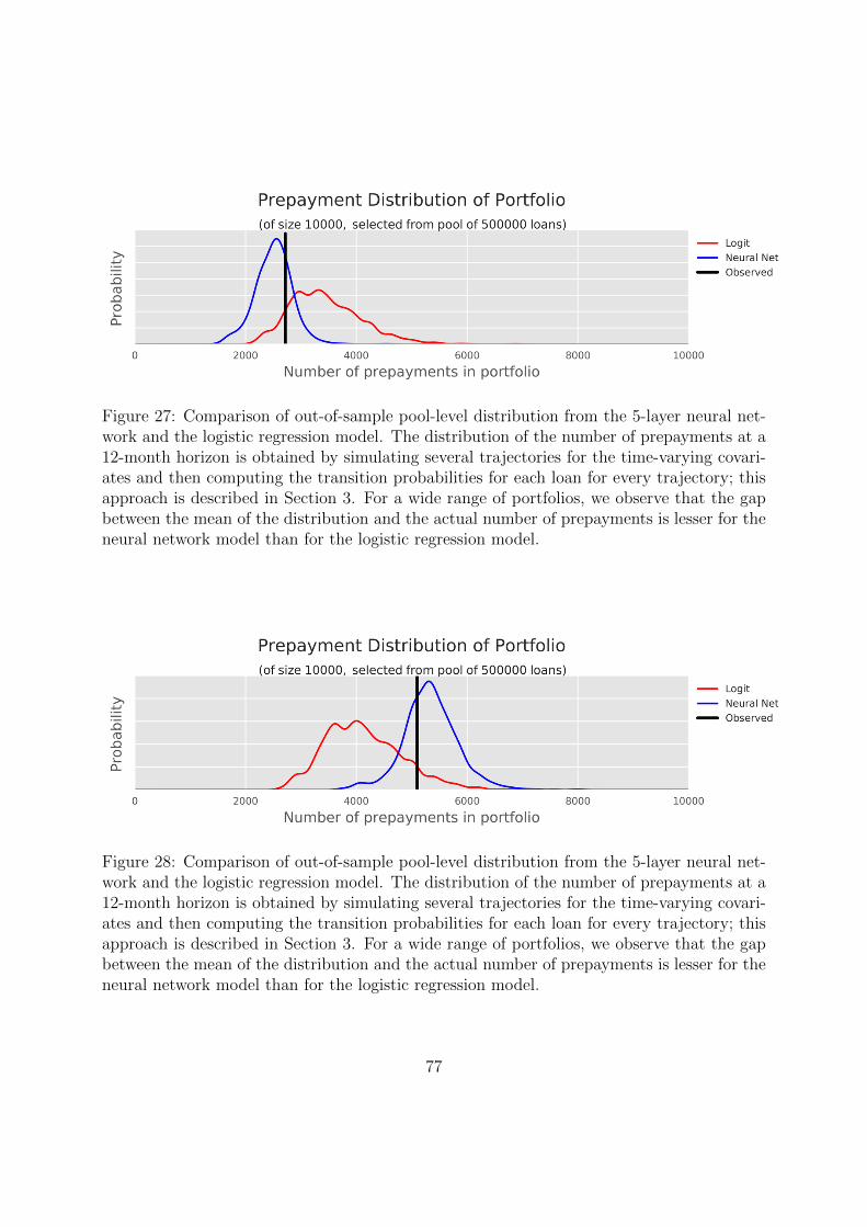
Figure 27: Comparison of out-of-sample pool-level distribution from the 5-layer neural net-work and the logistic regression model. The distribution of the number of prepayments at a12-month horizon is obtained by simulating several trajectories for the time-varying covari-ates and then computing the transition probabilities for each loan for every trajectory; thisapproach is described in Section 3. For a wide range of portfolios, we observe that the gapbetween the mean of the distribution and the actual number of prepayments is lesser for theneural network model than for the logistic regression model.

Figure 28: Comparison of out-of-sample pool-level distribution from the 5-layer neural net-work and the logistic regression model. The distribution of the number of prepayments at a12-month horizon is obtained by simulating several trajectories for the time-varying covari-ates and then computing the transition probabilities for each loan for every trajectory; thisapproach is described in Section 3. For a wide range of portfolios, we observe that the gapbetween the mean of the distribution and the actual number of prepayments is lesser for theneural network model than for the logistic regression model.

77

References

Agarwal, S., B. Ambrose & Y. Yildirim (2015), ‘The subprime virus’, Real Estate Economics

43(4), 891–915.

Agarwal, Sumit, Gene Amromin, Itzhak Ben-David, Souphala Chomsisengphet & Douglas

Evanoff (2011), ‘The role of securitization in mortgage renegotiation’, Journal of Fi-

nancial Economics 102, 559–578.

Agarwal, Sumit, Yan Chang & Abdullah Yavaz (2012), ‘Adverse selection in mortgage secu-

ritization’, Journal of Financial Economics 105, 640–660.

Albertini, F. & E. Sontag (1993), ‘For neural networks, function determines form’, Neural

Networks 6, 975–990.

Anenberg, E. & E. Kung (2014), ‘Estimates of the size and source of price declines due to

nearby foreclosures’, American Economic Review 104(8), 2527–51.

Azizpour, S., K. Giesecke & G. Schwenkler (2017), Exploring the sources of default clustering.

Journal of Financial Economics, forthcoming.

Bansal, R. & S. Viswanathan (1993), ‘No arbitrage and arbitrage pricing: A new approach’,

The Journal of Finance 48(4), 1231–1262.

Bengio, Y. & Y. LeCun (2007), ‘Scaling learning algorithms towards AI’, Large-scale kernel

machines 34(5).

Boudoukh, J., R. Whitelaw, M. Richardson & R. Stanton (1997), ‘Pricing mortgage-backed

securities in a multifactor interest rate environment’, Review of Financial Studies

10(2), 405–446.

Brown, S., W. Goetzmann & A. Kumar (1998), ‘The dow theory: William peter hamilton’s

track record reconsidered’, The Journal of Finance 53(4), 1311–1333.

Butaru, F., Q. Chen, B. Clark, S. Das, A. Lo & A. Siddique (2016), ‘Risk and risk manage-

ment in the credit card industry’, Journal of Banking and Finance 72, 218–239.

Campbell, J., S. Gigli & P. Pathak (2011), ‘Forced sales and house prices’, American Eco-

nomic Review 101(5), 2108–2131.

Campbell, John Y., Jens Hilscher & Jan Szilagyi (2008), ‘In search of distress risk’, Journal

of Finance LXIII(6), 2899–2939.

78

Campbell, T. & J. Dietrich (1983), ‘The determinants of default on insured conventional

residential mortgage loans’, Journal of Finance 38, 1569–1581.

Chernov, M., B. Dunn & F. Longstaff (2016), Macroeconomic-driven prepayment risk and

the valuation of mortgage-backed securities. Review of Financial Studies, forthcoming.

Cunningham, D. & P. Hendershott (1986), ‘Pricing fha mortgage default insurance’, Housing

Finance Review 13, 373–392.

Cunningham, Donald F. & Charles A. Capone (1990), ‘The relative termination experience

of adjustable to fixed-rate mortgages’, The Journal of Finance 45(5), 1687–1703.

Curley, A. & J. Guttentag (1974), ‘The yield on insured residential mortgages’, Explorations

in Economic Research 1, 114–161.

Curley, Anthony J. & Jack M. Guttentag (1977), ‘Value and yield risk on outstanding insured

residential mortgages’, The Journal of Finance 32(2), 403–412.

Deng, Y. (1997), ‘Mortgage termination: An empirical hazard model with a stochastic term

structure’, The Journal of Real Estate Finance and Economics 14(3), 309–331.

Deng, Y., J. Quigley & R. Van Order (2000), ‘Mortgage terminations, heterogeneity, and

the exercise of mortgage options’, Econometrica 68(2), 275–307.

Dixon, M., D. Klabjan & J.H. Bang (2016), Classification-based financial markets prediction

using deep neural networks. Working Paper, Northwestern University.

Donaldson, R. & M. Kamstra (1996), ‘A new dividend forecasting procedure that rejects

bubbles in asset price: The case of the 1929’s stock crash’, The Review of Financial

Studies 9(2), 333–383.

Duffie, D., L. Saita & K. Wang (2007), ‘Multi-period corporate default prediction with

stochastic covariates’, Journal of Financial Economics 83, 635665.

Eldan, R. & O. Shamir (2016), ‘The power of depth for feedforward neural networks’, Con-

ference on Learning Theory (COLT) .

Elliott, G. & A. Timmermann (2008), ‘Economic forecasting’, Journal of Economic Litera-

ture 46(1), 3–56.

Elul, Ronel, Nicholas S. Souleles, Souphala Chomsisengphet, Dennis Glennon & Robert Hunt

(2010), ‘What ”triggers” mortgage default?’, The American Economic Review, Papers

and Proceedings 100(2), 490–494.

79

Episcopos, A., A. Pericli & J. Hu (1998), ‘Commercial mortgage default: A comparison of

logit with radial basis function networks’, Journal of Real Estate Finance and Economics

17(2), 163–178.

Foote, Christopher, Kristopher Gerardi, Lorenz Goette & Paul Willen (2010), ‘Reducing

foreclosures: No easy answers’, NBER Macroeconomics Annual 24(1), 89–138.

Frame, Scott, Kristopher Gerardi & Paul Willen (2015), The failure of supervisory stress

testing: Fannie mae, freddie mac, and ofheo. Working Paper, Federal Reserve Bank of

Boston, 2015.

Gau, G. (1978), ‘A taxonomic model for the risk-rating of residential mortgages’, The Journal

of Business 51(4), 687–706.

Gelman, A. & J. Hill (2007), Data Analysis Using Regression and Multilevel/Hierarchical

Models, Cambridge University Press, Cambridge.

Goodfellow, Ian, Yoshua Bengio & Aaron Courville (2016), Deep Learning, MIT Press.

Granger, C. (1995), ‘Modelling nonlinear relationships between extended-memory variables’,

Econometrica 63(2), 265–279.

Green, J. & J. Shoven (1986), ‘The effects of interest rates on mortgage prepayments’,

Journal of Money, Credit and Banking 18, 41–59.

Harding, J., E. Rosenblatt & V. Yao (2009), ‘The contagion effect of foreclosed properties’,

Journal of Urban Economics 66, 164–178.

Heaton, J. B., N. G. Polson & J. H. Witte (2016), Deep portfolio theory. Working Paper,

University of Chicago.

Hornik, K. (1991), ‘Approximation capabilities of multilayer feedforward networks’, Neural

Networks 4(2), 251–257.

Hornik, K., M. Stinchcombe & H. White (1989), ‘Multilayer feedforward networks are uni-

versal approximators’, Neural Networks 2(5), 359366.

Hutchinson, J., A. Lo & T. Poggio (1994), ‘A nonparametric approach to pricing and hedging

derivative securities via learning networks’, Journal of Finance 49, 851–889.

Jiang, W., A. Nelson & E. Vytlacil (2014), ‘Securitization and loan performance: A contrast

of ex ante and ex post relations in the mortgage market’, Review of Financial Studies

27, 454–483.

80

Khandani, A., A. Kim & A. Lo (2010), ‘Consumer credit-risk models via machine-learning

algorithms’, Journal of Banking and Finance 34(11), 2767–2787.

Kuan, C. & H. White (1994), ‘Artificial neural networks: an econometric perspective’, Econo-

metric reviews 13(1), 1–91.

Lee, T., H. White & C. Granger (1993), ‘Testing for neglected nonlinearity in time-series

models’, Journal of Econometrics 56, 269–290.

Lin, Z., E. Rosenblatt & V. Yao (2009), ‘Spillover effects of foreclosures on neighborhood

property values’, Journal of Real Estate Finance and Economics 38(4), 387–407.

Mallat, S. (2016), ‘Understanding deep convolutional networks’, Philosophical Transactions

of the Royal Society A 374(2065).

Maxam, C. & M. LaCour-Little (2001), ‘Applied nonparametric regression techniques: Es-

timating prepayments on fixed-rate mortgage-backed securities’, Journal of Real Estate

Finance and Economics 32(2), 139–160.

McConnell, J. & M. Singh (1994), ‘Rational prepayments and the valuation of collateralized

mortgage obligations’, The Journal of Finance 49(3), 891–921.

Montufar, G., R. Pascanu, K. Cho & Y. Bengio (2014), ‘On the number of linear regions of

deep neural networks’, Advances in Neural Information Processing Systems pp. 2924–

2932.

Ngiam, J., A. Coates, A. Lahiri, B. Prochnow, Q. Le & A. Ng (2011), ‘On optimization

methods for deep learning’, International Conference on Machine Learning (ICML-11)

pp. 265–272.

Rajan, U., A. Seru & V. Vig (2015), ‘The failure of models that predict failure: Distance,

incentives and defaults’, Journal of Financial Economics 111, 237–260.

Richard, Scott & Richard Roll (1989), ‘Prepayments on fixed-rate mortgage-backed securi-

ties’, Journal of Portfolio Management 15, 73–82.

Schwartz, E. & W. Torous (1989), ‘Prepayment and the valuation of mortgage-backed secu-

rities’, The Journal of Finance 44(2), 375–392.

Schwartz, E. & W. Torous (1993), ‘Mortgage prepayment and default decisions: A pois-

son regression approach’, Journal of the American Real Estate and Urban Economics

Association 21(4), 431–449.

81

Shumway, T. (2001), ‘Forecasting bankruptcy more accurately: A simple hazard model’,

Journal of Business 74(1), 101–124.

Sirignano, J. (2016), Deep learning for limit order books. Working Paper, University of

Illinois at Urbana-Champaign.

Sirignano, J., G. Tsoukalas & K. Giesecke (2016), ‘Large-scale loan portfolio selection’,

Operations Research 64, 1239–1255.

Sirignano, J. & K. Giesecke (2015), Risk analysis for large pools of loans. Management

Science, forthcoming.

Srivastava, N., G. Hinton, A. Krizhevsky & I. Sutskever (2014), ‘Dropout: A simple way to

prevent neural networks from overfitting’, The Journal of Machine Learning Research

15(1), 1929–1958.

Stanton, R. & N. Wallace (2011), ‘The bear’s lair: Index credit default swaps and the

subprime mortgage crisis’, Review of Financial Studies 24(10), 3250–3280.

Sussmann, H. (1992), ‘Uniqueness of the weights for minimal feedforward nets with a given

input-output map’, Neural Networks 5(4), 589–593.

Swanson, N. & H. White (1997), ‘A model selection approach to real-time macroeconomic

forecasting using linear models and artificial neural networks’, The Review of Economics

and Statistics 79(4), 540–550.

Telgarsky, M. (2016), ‘Benefits of depth in neural networks’, Conference on Learning Theory

(COLT) .

Titman, S. & W. Torous (1989), ‘Valuing commercial mortgages: An empirical investigation

of the contingent-claims approach to pricing risky debt’, Journal of Finance 44(2), 345–

373.

Towe, C. & C. Lawley (2013), ‘The contagion effect of neighboring foreclosures’, American

Economic Journal: Economic Policy 5(2), 313–35.

Vandell, K. (1978), ‘Default risk under alternative mortgage instruments’, The Journal of

Finance 33(5), 1279–1296.

Vandell, K. (1992), ‘Predicting commercial mortgage foreclosure experience’, Journal of the

American Real Estate and Urban Economics Association 20, 55–88.

82

von Furstenberg, G. (1969), ‘Default risk on fha-insured home mortgages as a function of

the terms of financing: A quantitative analysis’, Journal of Finance 24, 459–477.

Webb, Bruce G. (1982), ‘Borrower risk under alternative mortgage instruments’, The Journal

of Finance 37(1), 169–183.

White, H. (1989), ‘Some asymptotic results for learning in single hidden layer feedforward

networks’, Journal of the American Statistical Association 84(408), 1008–1013.

White, Halbert (1989a), ‘Learning in artificial neural networks: A statistical perspective’,

Neural Computation 1(4), 425–464.

White, Halbert (1989b), ‘Some asymptotic results for learning in single hidden-layer feedfor-

ward network models’, Journal of the American Statistical Association 84(408), 1003–

1013.

White, Halbert (1992), Artificial Neural Networks: Approximation and Learning Theory,

Blackwell Publishers, Inc., Cambridge, MA, USA.

83