Deep Learning-Based Autonomous Scanning Electron Microscope

Jonggyu Jang1, Hyeonsu Lyu1, Hyun Jong Yang2,3, Moohyun Oh3, and Junhee Lee4

Abstract— By virtue of their ultra high resolution, scanningelectron microscopes (SEMs) are essential to study topography,morphology, composition, and crystallography of materials,and thus are widely used for advanced researches in physics,chemistry, pharmacy, geology, etc. The major hindrance ofusing SEMs is that obtaining high quality images from SEMsrequires a professional control of many control parameters.Therefore, it is not an easy task even for an experiencedresearcher to get high quality sample images without any helpfrom SEM experts. In this paper, we propose and implement adeep learning-based autonomous SEM machine, which assessesimage quality and controls parameters autonomously to gethigh quality sample images just as if human experts do. Thisworld’s first autonomous SEM machine may be the first stepto bring SEMs, previously used only for advanced researchesdue to its difficulty in use, into much broader applications suchas education, manufacture, and mechanical diagnosis, whichare previously meant for optical microscopes.

Index Terms— Scanning electron microscope (SEM), deepreinforcement learning (DRL), deep deterministic policy gra-dient (DDPG), advanced robotics

I. INTRODUCTION

A scanning electron microscope (SEM) produces three-dimensional surface images of a sample from secondaryelectrons generated by projecting focused electron beamson the sample surface. The output quality of sample imagesis highly susceptible to many interrelated SEM parameterssuch as working distance, brightness, magnification, con-trast, etc. Furthermore, an optimal set of these parametersis dependent on the direction and height of the samplestage, intensity of illumination, types of samples, etc. Hence,only well-trained SEM experts can find optimal parameterswithin feasible time. As a consequence, despite of their ultrahigher resolution, SEMs have been used only for limited usecases such as advanced researches in physics, chemistry,geology, etc. In this paper, we propose and implement afully autonomous machine which can evaluate the quality of

This work was supported in part by the MSIT(Ministry of Science andICT), Korea, under the ITRC(Information Technology Research Center)support program(IITP-2020-2017-0-01635) supervised by the IITP(Institutefor Information & communications Technology Promotion), and the Tech-nology Innovation Program (or Industrial Strategic Technology Develop-ment Program (20005526, Development of Artificial Intelligence ScanningElectron Microscope) funded By the Ministry of Trade, Industry & En-ergy(MOTIE, Korea).

1Jonggyu Jang and Hyeonsu Lyu are with the School of Elec-trical and Computer Engineering, Ulsan National Institute of Scienceand Technology (UNIST), Ulsan 44919, Republic of Korea, (e-mail:{jonggyu,hslyu}@unist.ac.kr)

2Hyun Jong Yang (corresponding author) is with department of electricalengineering, Pohang University of Science and Technology (POSTECH),Pohang 37673, Republic of Korea, (email: hyunyang@postech.ac.kr)

3Hyun Jong Yang and Moohyun Oh are with Egovid Inc., Ulsan 44919,Republic of Korea, (e-mail: {hjyang,mhoh}@egovid.com)

4Junhee Lee is with Coxem Co. Ltd, Daejeon 34025, Republic of Korea,(e-mail: junhee@coxem.com)

Fig. 1: Examples of the gradient and variance for Grid andTinball samples, which are normalized into the range of[0, 10].sample images and control SEM parameters just as highly-skilled human experts do.

A. Related Works1) Existing Autofocus Schemes: Recently developed

SEMs often have an ‘autofocus’ (AF) functionality that au-tomatically controls the SEM parameters to improve imagequality. In the literature [1], [2], AF schemes have beenproposed to control one or multiple SEM parameters, withthe aim of maximizing various image quality metrics definedbased on mathematical functions such as the variance orspatial gradient of pixel values. However, there are fataltheoretical limitations in the existing image quality metricsin some cases, such as recognizing the picture of whitenoise as a high quality image because of the high varianceand spatial gradients of its pixel values. For instance, Fig.1 depicts the variance and average gradient of the pixelvalues for two different sample types, Grid and Tinball,which are normalized into the range of [0, 10]. As seen,the gradient and variance of the out-focused images are stillhigh and not distinguishable from the well-focused cases.Consequently, no existing AF scheme can measure imagequality while considering both the whole and partial partsof the sample, and consistently perform well for varioussample types, sample stage heights, scales, etc. In reality, theexisting AF functions are used merely to set initial values ofthe SEM parameters, and it still requires fine manual controlof SEM experts to obtain a high-quality image.

2) Deep Learning for Microscope: Deep learning pow-ered by deep neural networks (DNNs) and abundant trainingdata has shown its miraculous capability in overdetermined,stationary, and deterministic problems such as classifyingimages, optimizing digital filters, solving an NP-hard sta-tionary problem, etc. Recently, deep learning has expandedits application to SEM image classification and analysis [3],[4]. While the majority of the literature have studied deeplearning as a SEM image classifier or analyzer, our previousstudy [5] is the only work showing that deep learningcan be potentially used as a SEM parameter controller toget high quality images. However, only the image qualityprediction problem is addressed in [5], and no parameter

2020 IEEE/RSJ International Conference on Intelligent Robots and Systems (IROS)October 25-29, 2020, Las Vegas, NV, USA (Virtual)

978-1-7281-6211-9/20/$31.00 ©2020 IEEE 2886

control scheme is proposed. Though our scope is restrictedto SEMs, there also have been few works studying deeplearning as a controller even for optical microscopes [6].

B. Challenges

To implement a deep learning-based autonomous SEMmachine, there are three major challenges:

• A new image quality evaluation metric should be de-fined, which overcomes the known critical limitationsof the existing metrics and shows robust accuracy fora variety of environments such as sample types, heightof the sample stage, magnifications, etc.

• Instead of simple supervised learning, a well-designedreinforcement learning-based machine should be de-signed, which controls the SEM parameters adaptingitself to varying environments.

• A full integrated system should be implemented in-cluding the following parts: i) softwares and hardwaresinterconnecting a SEM and a computing node; ii) deeplearning-based software machines at the computingnode, which evaluates image quality and controls SEMparameters autonomously.

C. Contributions

Our main contributions are summarized as follows:

• To overcome the known limitations of the existingAF metrics, we develop a new metric to evaluateSEM images based on highly-qualified SEM experts’assessment on the quality of images.

• We develop a reinforcement learning-based controlmachine which controls SEM parameters in order toobtain high quality images autonomously. Our controlmachine employs the newly developed metric as itsreward, and adapts itself to the change in environmentsincluding sample types, heights of the sample stage,magnifications, etc., yielding robust control accuracy.Since human experts cannot give the control machinetheir assessment results on a real-time basis to com-pute the reward online, we also develop a supervisedlearning-based scoring machine that mimics humanexperts to evaluate image quality.

• To train our scoring and control machines, we pro-pose a method to construct a dataset composed ofexperts’ assessment scores, sample images, and controlparameters. To make our machines perform robust forvarying environments with limited amount of dataset,we design the reward by combining experts’ scores andthe existing AF metrics.

• We renovate an off-the-shelf SEM, EM-30, and im-plement the world’s first autonomous SEM machine.Specifically, we develop a software/hardware to enablethe SEM and the computing node to communicate witheach other. We implement a deep learning-based soft-ware/hardware system at the computing node, whichanalyzes input images from the SEM and generatescommands to the SEM for adjusting parameters. Our

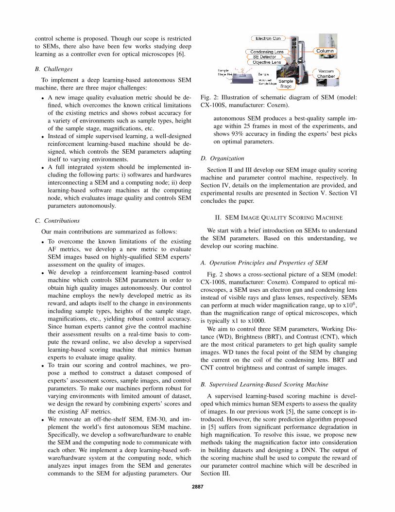
Fig. 2: Illustration of schematic diagram of SEM (model:CX-100S, manufacturer: Coxem).

autonomous SEM produces a best-quality sample im-age within 25 frames in most of the experiments, andshows 93% accuracy in finding the experts’ best pickson optimal parameters.

D. Organization

Section II and III develop our SEM image quality scoringmachine and parameter control machine, respectively. InSection IV, details on the implementation are provided, andexperimental results are presented in Section V. Section VIconcludes the paper.

II. SEM IMAGE QUALITY SCORING MACHINE

We start with a brief introduction on SEMs to understandthe SEM parameters. Based on this understanding, wedevelop our scoring machine.

A. Operation Principles and Properties of SEM

Fig. 2 shows a cross-sectional picture of a SEM (model:CX-100S, manufacturer: Coxem). Compared to optical mi-croscopes, a SEM uses an electron gun and condensing lensinstead of visible rays and glass lenses, respectively. SEMscan perform at much wider magnification range, up to x106,than the magnification range of optical microscopes, whichis typically x1 to x1000.

We aim to control three SEM parameters, Working Dis-tance (WD), Brightness (BRT), and Contrast (CNT), whichare the most critical parameters to get high quality sampleimages. WD tunes the focal point of the SEM by changingthe current on the coil of the condensing lens. BRT andCNT control brightness and contrast of sample images.

B. Supervised Learning-Based Scoring Machine

A supervised learning-based scoring machine is devel-oped which mimics human SEM experts to assess the qualityof images. In our previous work [5], the same concept is in-troduced. However, the score prediction algorithm proposedin [5] suffers from significant performance degradation inhigh magnification. To resolve this issue, we propose newmethods taking the magnification factor into considerationin building datasets and designing a DNN. The output ofthe scoring machine shall be used to compute the reward ofour parameter control machine which will be described inSection III.

2887

1) Dataset: While the range of BRT and CNT values inwhich SEM images are clearly visible is relatively wide,the range of such WD values is very narrow. Hence, manydifferent WD values should be considered in the datasetconstruction. SEM images are collected in the dataset forvarious (WD, BRT, CNT) values so that both out-focusedand focused images are sufficiently included in the dataset.

Several highly-qualified SEM experts labeled perfectlyfocused images by 10 points, and totally unrecognizableimages such as a noise image by 0 point. Though it isclear for 10-point and 0-point cases, it is not an easy taskto evaluate images which are focused to some extent butnot perfectly. For each sample type and magnification, theSEM experts selected several reference images representing1-point to 9-point cases. Then, the other images were labeledin comparison to these representative reference images. Notethat how accurately images are labeled in the range of 1point to 9 points is not critical in constructing the dataset,since the goal is to get 10-point images after all avoiding0-point cases.

Though finer granularity in the scoring range [0, 10] mayhelp our parameter control machine adjust the parametersmore carefully, it may be impossible for human expertsto recognize very small difference in the image quality.To compromise, we employed integer scores of 0, 1, ...,10. In Section III, we will introduce a new metric tocomplement the weakness of this experts’ scoring, suchas human mistakes, discrete score values, theoretically notperfect definition of the 1 to 9 points, by combining experts’scores with the existing AF metrics.

Finally, an equal number of images were collected foreach magnification of x(500, 1000, 2000, 5000, 10000),because the DNN used in our parameter control machinecould be biased if images at a particular magnification aredominating the other magnification cases.

2) Deep Neural Network Design: Our deep learning-based scoring machine architecture is illustrated in Fig. 3,which mimics human experts to evaluate the image qualityscore. In fact, if a DNN is excessively deep, i.e., it includesmany hidden layers, then it may show robust prediction ac-curacy even without the magnification value as an input forvarying magnification. However, unlike the DNN structurein [5], we propose to use a magnification value as an inputas well as a sample image in order to keep the computationalcomplexity feasible while enhancing the prediction accuracyfor varying magnification. To standardize the input format,an input image is cropped to be 240× 320-sized. In pursuitof enriching the training dataset, an image in the dataset iscropped randomly and flipped vertically and horizontallyto generate multiple training images. In the testing, the240×320-sized center block is cropped from an input image.

As seen from Fig. 3, we used ResNet18 [7]1 as an imageprocessing network, which extracts a 512× 1-sized featurevector from an input image.

1Although some other existing models such as ResNet50, ResNet101,VGG11, and VGG19 [8] perform also well, ResNet18 shows the bestcompromise between computation time and score prediction performance.

Fig. 3: Illustration of the proposed supervised learning-basedscoring machine.

To restrict the cardinality of the variable domain, themagnification value is normalized into [0,1]. Similarly, the512×1-dimensional feature vector passes through a nonlin-ear soft-max layer so that each element is normalized into[0,1]. Then, the soft-max layer output is augmented withthe normalized magnification value to form a 513× 1-sizedvector. This augmented vector passes through three fullyconnected network (FCN) layers, where the final output isthe predicted score.

Let us define our scoring machine as SCORE :R240×320 × R → R and the dataset as S. Formally, theinputs are defined as X ∈ R240×320 and MAG, where Xdenotes the pixel value matrix of an input image, and MAGis the normalized magnification. The elements of dataset Sare tuples of (X, MAG, ES), where ES denotes the experts’score. In the training, the DNN is updated such that thefollowing root-mean-square-error (RMSE) loss function isminimized:√√√√ 1

|S|∑

(X,MAG,ES)∈S

(ES− SCORE(X,MAG))2. (1)

III. PARAMETER CONTROL MACHINE FOR ADJUSTINGSEM PARAMETERS

In this section, our reinforcement learning-based param-eter control machine is presented, which controls the threeparameters of (WD, BRT, CNT) to get high quality imageautonomously. For continuous control of the parameters, thedeep deterministic policy gradient (DDPG) algorithm [9] isadapted with careful design of states, actions, and rewards.Since in each reinforcement step, it is not possible forhuman experts to give the machine their score for computingreward online, we utilize the output of our scoring machinedescribed in Section II, which predicts experts’ scores.Furthermore, we also exploit the existing AF metrics indesigning the reward to cope with cases unexplored in thetraining.

A. Notation of Variables

Let us denote WD, BRT, CNT, and the sample imageupdated at the t-th reinforced control step by p1,t, p2,t,p3,t, and Xt ∈ R240×320, respectively. Note that the sampleimage also changes as a consequence of the change inthe parameters. For notional convenience, the followingnotations are used: pt = [p1,t, p2,t, p3,t]

T ∈ R3; the upper

2888

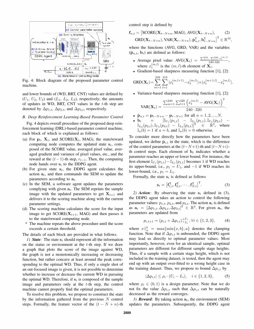
Fig. 4: Block diagram of the proposed parameter controlmachine.

and lower bounds of (WD, BRT, CNT) values are defined by(U1, U2, U3) and (L1, L2, L3), respectively; the amountsof updates in WD, BRT, CNT values in the t-th step aredenoted by ∆p1,t, ∆p2,t, and ∆p3,t, respectively.

B. Deep Reinforcement Learning-Based Parameter Control

Fig. 4 depicts overall procedure of the proposed deep rein-forcement learning (DRL)-based parameter control machine,each block of which is explained as follows:(a) For pt, Xt, and SCORE(Xt, MAG), the state/reward

computing node computes the updated state st, com-posed of the SCORE value, averaged pixel value, aver-aged gradient and variance of pixel values, etc., and thereward at the (t−1)-th step, rt−1. Then, the computingnode hands over st to the DDPG agent.

(b) For given state st, the DDPG agent calculates theaction at, and then commands the SEM to update theparameters according to at.

(c) In the SEM, a software agent updates the parameterscomplying with given at. The SEM reprints the sampleimage with the updated parameters to get Xt+1 anddelivers it to the scoring machine along with the currentparameter settings.

(d) The scoring machine calculates the score for the inputimage to get SCORE(Xt+1, MAG) and then passes itto the state/reward computing node.

* The machine repeats the above procedure until the scoreexceeds a certain threshold.

The details of each block are provided in what follows.1) State: The state st should represent all the information

on the status or environment at the t-th step. If we drawa graph that plots the score of the image against WD,the graph is not a monotonically increasing or decreasingfunction, but rather concave at least around the peak corre-sponding to the optimal WD. Thus, if only a single shot ofan out-focused image is given, it is not possible to determinewhether to increase or decrease the current WD in pursuingthe optimal WD. Therefore, if st is composed of the sampleimage and parameters only at the t-th step, the controlmachine cannot properly find the optimal parameters.

To resolve this problem, we propose to construct the stateby the information gathered from the previous N controlsteps. Formally, the feature vector of the (t − N + n)-th

control step is defined by

fn,t =[SCORE(Xt−N+n,MAG),AVG(Xt−N+n), (2)

GRD(Xt−N+n),VAR(Xt−N+n), pTn,t,b

Tt−N+n

]T ∈ R10,

where the functions (AVG, GRD, VAR) and the variables(pn,t, bt) are defined as follows:

• Average pixel value: AVG(Xt) =∑240

m=1

∑320l=1 x

(m,l)t

240·320 ,where x(m,l)t is the (m, l)-th element of Xt.

• Gradient-based sharpness measuring function [1], [2]:

GRD(Xt)=

239∑m=1

319∑l=1

|x(m,l+1)t −x(m,l)t |+|x(m+1,l)

t −x(m,l)t |.

• Variance-based sharpness measuring function [1], [2]:

VAR(Xt) =

∑240m=1

∑320l=1

(x(m,l)t − AVG(Xt)

)2240 · 320

.

• pn,t = pt−N+n − pt−N+1 for all n = 1, 2, ..., N .• bt = [IU1(p1,t) − IL1(p1,t), IU2(p2,t) −

IL2(p2,t), IU3

(p3,t) − IL3(p3,t)]

T ∈ R3, whereIa(b) = 1 if a = b, and Ia(b) = 0 otherwise.

To consider more directly how the parameters have beenupdated, we define pi,t in the state, which is the differenceof the control parameters at the (t−N+1)-th and (t−N+i)-th control steps. Each element of bt indicates whether aparameter reaches an upper or lower bound. For instance, thefirst element IU1

(p1,t)−IL1(p1,t) becomes 1 if WD reaches

its upper-bound, i.e., p1 = U1, and −1 if WD reaches itslower-bound, i.e., p1 = L1.

Formally, the state st is defined as follows

st =[fT1,t, f

T2,t, · · · , fT

N,t

]T. (3)

2) Action: By observing the state st defined in (3),the DDPG agent takes an action to control the followingparameter values: p1,t, p2,t, and p3,t. The action at is definedas at = [∆p1,t,∆p2,t,∆p3,t]

T ∈ R3. For given at, theparameters are updated from

pi,t+1 = (pi,t + ∆pi,t)⊥Ui

>Li,∀i ∈ {1, 2, 3}, (4)

where x⊥b>a = max{min{x, b}, a} denotes the clampingfunction. Note that if ∆pi,t is unbounded, the DDPG agentmay lead us directly to optimal parameter values. Mostimportantly, however, even for an identical sample, optimalparameters are different for different sample stage heights.Thus, if a sample with a certain stage height, which is notincluded in the training dataset, is tested, then the agent mayend up with an output over-fitted to a wrong height case inthe training dataset. Thus, we propose to bound ∆pi,t by

|∆pi,t| ≤ ρi · (Ui − Li), i ∈ {1, 2, 3}, (5)

where ρi ∈ (0, 1) is a design parameter. Note that we donot fix the value ∆pi,t such that ∆pi,t can be naturallydecreased as the reward converges.

3) Reward: By taking action at, the environment (SEM)updates the parameters. Subsequently, the DDPG agent

2889

receives the reward for that action from the state/rewardcomputing node as in Fig. 4. The reward is generally definedas a goal to maximize in DRL, such as winning rate,incomes, and game scores. Our goal is obviously to get animage with a high experts’ score. Thus, the reward shouldbe designed such that the output of our scoring machine ismaximized.

In reality, however, we have limited data in the trainingdataset. Hence, if some cases with stage heights and sampletypes, which are not included in the training dataset, areencountered, then there is a chance that the control per-formance is degraded or the DDPG agent gives an over-fitted output. Furthermore, score labeling cannot be perfectlyconsistent for many data, since it is done by human experts.

Thus, we design the reward also with supplementary de-terministic functions such as averaged gradient and varianceof the input pixel values, which played a role of measuringimage quality in the conventional studies. Supposedly, onemay think of the reward SCORE(Xt,MAG) + GRD(Xt) +VAR(Xt). Recall that our control machine terminates theprocedure if SCORE exceeds a certain threshold, say ω.Suppose that the DDPG has reached ω − ε in reward withan arbitrarily small number ε. If the DDPG tries to exceedω, then it is obvious that the future reward becomes 0.Since the ultimate goal of DRL is to maximize the futurereward, our DDPG will be trained with the aforementionedreward design such that it stays forever at a set of parametersproducing the reward of ω − ε.

As a remedy, we define the reward of the t-th step as

rt = SCORE(Xt+1,MAG)− SCORE(Xt,MAG) (6)+c1(GRD(Xt+1)−GRD(Xt))+c2(VAR(Xt+1)−VAR(Xt)),

where c1 and c2 are weight coefficients. Note that sincethe reward is defined by the change in the image qualityfrom the t-th to (t+1)-th step, the termination policy lookshazy to the DDPG agent during the training. Hence, theDDPG is simply trained such that the reward increases at anyinstance. Furthermore, this reward design results in robustdeep learning performance in different SEM hardwares,where the scale of the measurements on X can be differentunder different hardware settings.

4) State-Action Function (Actor DNN): In the conven-tional DDPG algorithm [9], an actor DNN is a function ofstate st, and designed to obtain the value of the action atin a continuous space. Specifically, if we denote the optimalaction as a∗t = A∗(st), then the actor DNN aims to estimateA∗(st). For the DNN parameter θ, the output of the actorDNN is denoted by as A(st;θ) .

5) Action-state-value Function (Critic DNN): By theBellman equation, the action-state-value function with pol-icy π and forgetting factor γ is defined as

Q(st,at) = Est+1,at+1,st+2,...

[ ∞∑n=t

γn−trn

](a)= E

st+1,at+1∼π[rt + γQπ(st+1,at+1)] . (7)

With the DNN parameter φ, the critic DNN outputs the esti-mate of Q(st+1,at+1), denoted by Q(st+1, A(st+1;θ);φ).

6) Training Objectives and Target DNN Parameters:From (7), the target value in update of the critic DNNis rt + γQ(st+1, A(st+1;θ);φ). Note that φ and θ arerecursively included in this target value. Hence, if φ andθ are trained for the DNNs to pursuit this target value, theyoften diverge during the training. Therefore, the conceptof target parameters is considered as in [10]. The targetDNN parameters for φ and θ are denoted by φ− and θ−,respectively. Then, the target value for the critic DNN updateis defined as

zt = rt + γQ(st+1, A(st+1;θ−);φ−). (8)

Therefore, the critic DNN parameter φ is updated to reducethe critic loss function, which is defined as

L(φ) = E δ2t , (9)

where δt = zt − Q(st,at;φ) represents the temporaldifference error.

On the other hand, the aim of the actor DNN A(st;θ) isto obtain an estimate of the optimal policy. Hence, the actorDNN parameter is updated to maximize the output of thecritic DNN, Q(st, A(st;θ);φ), with policy A(st;θ).

7) Exploration and Exploitation: The DDPG agent ei-ther randomly explores the environment to get more in-formation or exploits its best actions during training. Weemploy the ε-greedy policy for exploration and exploitation.Specifically, the action at is taken from

at =

{A(st;θ), with probability 1− εA(st;θ) + nt, otherwise,

(10)

where nt denotes additive Gaussian random noise, i.e., nt ∼N (0, σ2I3).

8) Prioritized Experience Replay: In the training, anexperience tuple et = (st,at, rt, st+1) is obtained aftereach control step. Because experience tuples of consecutivecontrol steps are highly correlated, the DNN parametersconverge slow during training. Therefore, we resolve thisissue by employing the prioritized experience replay (PER)scheme [11]. Let us denote the set of indices of experiencetuples stored in the replay buffer by D. Then, each of expe-rience tuples in the replay buffer is selected by probabilityPt to form a mini-batch R, where Pt is defined by

Pt =oκt∑j∈D o

κj

. (11)

Here, ot = |δt| and κ denote the priority of experience etand a hyper-parameter, respectively.

9) Training and Target DNN Update: For the updateof the target DNNs for given mini-batch R, we employ theimportant-sampling (IS) method such that the DNN updatescan be not over-fitted to the experiences which are frequentlyselected in R. Specifically, the IS weight wt for the t-th

2890

experience is defined by

wt =

(1

|D|1

Pt

)ζ, (12)

where ζ is a hyper-parameter. Then, the critic DNN param-eter φ is updated to minimize the loss function (9) by thestochastic gradient method with the IS weight (12) as

φ← φ + αφ

∑t∈R

wtδt∇φQ(st,at,φ), (13)

where αφ represents learning rate of the critic DNN.The actor DNN parameter θ is updated to obtain the

action policy A(st;θ) that maximizes the critic DNN outputQ(st, A(st;θ);φ) as follows:

θ ← θ + αθ

∑t∈R∇θA(st;θ)

(∇aQ(st,a;φ)|a=A(st;θ)

),

(14)where αθ denotes learning rate of the actor DNN.

On the other hand, the target DNN parameters are updatedby the soft target DNN update scheme [9] as follows:

θ− ← τθ + (1− τ)θ−, φ− ← τφ + (1− τ)φ−, (15)

where τ � 1 is a hyper-parameter.10) DNN Structure: The actor and critic DNNs have

(input size, output size) of (10N , 3) and (10N + 3, 1),respectively. Since the input of the actor/critic network isa simple feature vector with no spatial correlation unlikeimages, the control machine can be operated effectivelyenough without complicated network design. The critic andactor DNNs are designed to have the same hidden layers ofsize of 256, 512, 512, 512, 512 and 256 neurons, and havethe same ReLU activation function.

The overall proposed DRL algorithm is summarized inAlgorithm 1.

IV. IMPLEMENTATION OF THE AUTONOMOUS SEM

Fig. 5 shows the overall implementation of our au-tonomous SEM. The SEM software named ‘NanoStation’saves the SEM image and the current SEM parameters inimage and text files, respectively in the parameter controlmachine (‘ (a)’ in Fig. 5). After reading the saved files, thescoring machine (‘(b)’ in Fig. 5) and state/reward computingnode (‘(c) in Fig. 5) calculate the score of the image andstate/reward, respectively. The parameter control machinereads the calculated score, state, and reward to calculatethe action value and write the calculated action value ina text file (‘(d)’ in Fig. 5). A software named ‘MiddleClient’ transmits the contents of that txt file to NanoStation(‘(e)’ in Fig. 5). The SEM hardware controls the parametercomplying with the message from Middle Client (‘(f)’ inFig. 5), and prints a new image to deliver it to NanoStation(‘(g)’ in Fig. 5).

A. SEM Hardware Specification

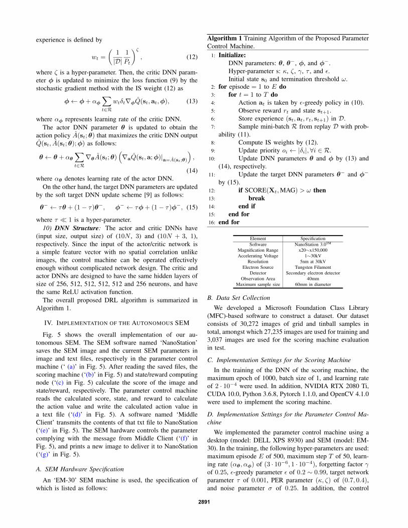
An ‘EM-30’ SEM machine is used, the specification ofwhich is listed as follows:

Algorithm 1 Training Algorithm of the Proposed ParameterControl Machine.

1: Initialize:DNN parameters: θ, θ−, φ, and φ−.Hyper-parameter s: κ, ζ, γ, τ , and ε.Initial state s0 and termination threshold ω.

2: for episode = 1 to E do3: for t = 1 to T do4: Action at is taken by ε-greedy policy in (10).5: Observe reward rt and state st+1.6: Store experience (st,at, rt, st+1) in D.7: Sample mini-batch R from replay D with prob-

ability (11).8: Compute IS weights by (12).9: Update priority oi ← |δi|,∀i ∈ R.

10: Update DNN parameters θ and φ by (13) and(14), respectively.

11: Update the target DNN parameters θ− and φ−

by (15).12: if SCORE(Xt,MAG) > ω then13: break14: end if15: end for16: end for

Element SpecificationSoftware NanoStation 3.0TM

Magnification Range x20∼x150,000Accelerating Voltage 1∼30kV

Resolution 5nm at 30kVElectron Source Tungsten Filament

Detector Secondary electron detectorObservation Area 40mm

Maximum sample size 60mm in diameter

B. Data Set Collection

We developed a Microsoft Foundation Class Library(MFC)-based software to construct a dataset. Our datasetconsists of 30,272 images of grid and tinball samples intotal, amongst which 27,235 images are used for training and3,037 images are used for the scoring machine evaluationin test.

C. Implementation Settings for the Scoring Machine

In the training of the DNN of the scoring machine, themaximum epoch of 1000, batch size of 1, and learning rateof 2 · 10−4 were used. In addition, NVIDIA RTX 2080 Ti,CUDA 10.0, Python 3.6.8, Pytorch 1.1.0, and OpenCV 4.1.0were used to implement the scoring machine.

D. Implementation Settings for the Parameter Control Ma-chine

We implemented the parameter control machine using adesktop (model: DELL XPS 8930) and SEM (model: EM-30). In the training, the following hyper-parameters are used:maximum episode E of 500, maximum step T of 50, learn-ing rate (αθ, αφ) of (3 · 10−6, 1 · 10−4), forgetting factor γof 0.25, ε-greedy parameter ε of 0.2 ∼ 0.99, target networkparameter τ of 0.001, PER parameter (κ, ζ) of (0.7, 0.4),and noise parameter σ of 0.25. In addition, the control

2891

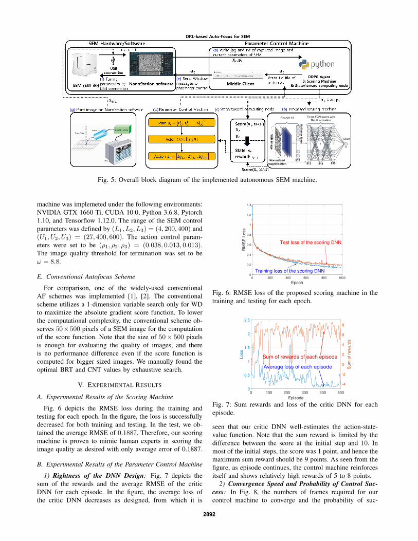
Fig. 5: Overall block diagram of the implemented autonomous SEM machine.

machine was implemeted under the following environments:NVIDIA GTX 1660 Ti, CUDA 10.0, Python 3.6.8, Pytorch1.10, and Tensorflow 1.12.0. The range of the SEM controlparameters was defined by (L1, L2, L3) = (4, 200, 400) and(U1, U2, U3) = (27, 400, 600). The action control param-eters were set to be (ρ1, ρ2, ρ3) = (0.038, 0.013, 0.013).The image quality threshold for termination was set to beω = 8.8.

E. Conventional Autofocus Scheme

For comparison, one of the widely-used conventionalAF schemes was implemented [1], [2]. The conventionalscheme utilizes a 1-dimension variable search only for WDto maximize the absolute gradient score function. To lowerthe computational complexity, the conventional scheme ob-serves 50×500 pixels of a SEM image for the computationof the score function. Note that the size of 50× 500 pixelsis enough for evaluating the quality of images, and thereis no performance difference even if the score function iscomputed for bigger sized images. We manually found theoptimal BRT and CNT values by exhaustive search.

V. EXPERIMENTAL RESULTS

A. Experimental Results of the Scoring Machine

Fig. 6 depicts the RMSE loss during the training andtesting for each epoch. In the figure, the loss is successfullydecreased for both training and testing. In the test, we ob-tained the average RMSE of 0.1887. Therefore, our scoringmachine is proven to mimic human experts in scoring theimage quality as desired with only average error of 0.1887.

B. Experimental Results of the Parameter Control Machine

1) Rightness of the DNN Design: Fig. 7 depicts thesum of the rewards and the average RMSE of the criticDNN for each episode. In the figure, the average loss ofthe critic DNN decreases as designed, from which it is

0 200 400 600 800 1000

Epoch

0

0.2

0.4

0.6

0.8

1

1.2

1.4

RM

SE

Lo

ss

Test loss of the scoring DNN

Training loss of the scoring DNN

Fig. 6: RMSE loss of the proposed scoring machine in thetraining and testing for each epoch.

0 100 200 300 400 500

Episode

0

0.5

1

1.5

2

2.5

Loss

-4

-2

0

2

4

6

8

Sum

of

rew

ard

s

Average loss of each episode

Sum of rewards of each episode

Fig. 7: Sum rewards and loss of the critic DNN for eachepisode.

seen that our critic DNN well-estimates the action-state-value function. Note that the sum reward is limited by thedifference between the score at the initial step and 10. Inmost of the initial steps, the score was 1 point, and hence themaximum sum reward should be 9 points. As seen from thefigure, as episode continues, the control machine reinforcesitself and shows relatively high rewards of 5 to 8 points.

2) Convergence Speed and Probability of Control Suc-cess: In Fig. 8, the numbers of frames required for ourcontrol machine to converge and the probability of suc-

2892

Fig. 8: Number of frames required for converge and prob-ability of successful control under various environmentsettings.

sample Scheme Magnification RMSE of WD Prob. of successfulBRT & CNT control

Avg.Score

Grid Proposed

500 0.2267 1.0000 9.53531000 0.1893 0.9796 9.25352000 0.1324 1.0000 9.55595000 0.0932 1.0000 9.0366

Conventional 0.3681 - 7.0182

Tinball Proposed

500 0.1292 1.0000 9.37481000 0.1034 1.0000 9.27492000 0.0813 1.0000 9.15045000 0.0718 1.0000 9.3766

Conventional 0.2153 - 7.5945

TABLE I: Parameter control accuracy and the average scoreafter the control.

cessful controls are depicted for various magnifications oftinball and grid samples. It is seen that the proposed schemerequires much less frames than the conventional schemeuntil converge, while having higher probability of success.In addition, the proposed scheme performs consistentlyunder various environment settings except for ‘grid withmagnification of 5000’. This is because images of the gridsample in high magnification sometimes capture hollowparts of the sample, i.e., there is no feature on the capturedimages.

3) Control Accuracy: Table I summarizes the controlaccuracy of the proposed control machine and the averagescore after the control. In general, it becomes more difficultto find the optimal WD value in high magnification. As seenfrom the table, our control machine even with the highestmagnification shows higher accuracy in finding the optimalWD than the conventional scheme, even though the RMSEof the conventional scheme is averaged across the entiremagnification range. Unlike WD, we can get high qualityimages for relatively wide ranges of BRT and CNT values.As seen from the table, our control machine successfullyadjusts BRT and CNT to make them fall into the highquality ranges with almost 100% probability. Finally, as seenfrom the last column of the table, the average score afterthe control significantly surpasses that of the conventionalscheme for both the sample types under all the magnificationsetups.

4) Exemplary Results: Fig. 9 shows examples of sampleimages before and after our parameter control for fourdifferent magnification setups and two different sampletypes. As seen from the figure, the images after the controllooks almost like those of experts’ best picks.

Fig. 9: Control result examples for Grid and Tinball sampletypes.

VI. CONCLUSION

An autonomous SEM has been implemented by proposingand implementing a image quality scoring and parametercontrol machines. Our autonomous SEM can produce highquality images, to which human experts would give 9 pointsout of 10 points. Therefore, it can be said that our machinecan deal with the SEM just as if human experts do. Usingour scoring and parameter control machines, SEMs becomeextremely easy to use and thereby can replace opticalmicroscopes in a variety of applications such as education,mechanical diagnosis, and manufacture. Exemplary videoresults of our implementation experiments can be found inthe following link: https://youtu.be/MvSaoPQvDdo.

REFERENCES

[1] A. Santos, C. O. D. Solorzano, J. J. Vaquero, J. M. Pena, N. Malpica,and F. D. Pozo, “Evaluation of autofocus functions in molecularcytogenetic analysis,” Journal of Microscopy, vol. 188, 1997.

[2] F. C. A. Groen, I. T. Young, and G. Ligthart, “A comparison ofdifferent focus functions for use in autofocus algorithms,” Cytometry,vol. 6, no. 2, pp. 81–91, 1985.

[3] M. H. Modarres, R. Aversa, S. Cozzini, R. Ciancio, A. Leto, andG. P. Brandino, “Neural network for nanoscience scanning electronmicroscope image recognition,” Scientific Reports, vol. 7, 2017.

[4] C. D. Nobili and S. Cozzini, “Deep learning for nanoscience scanningelectron microscope image recognition,” Master in High PerformanceComputing (MHPC), 2017.

[5] H. Kim, M. Oh, H. Lee, J. Jang, M. U. Kim, H. J. Yang, M. Ryoo, andJ. Lee, “Deep-learning based autofocus score prediction of scanningelectron microscope,” in Microscopy and Microanalysis (M&M),2019.

[6] H. Pinkard, Z. Phillips, A. Babakhani, D. A. Fletcher, and L. Waller,“Deep learning for single-shot autofocus microscopy,” Optica, vol. 6,no. 6, pp. 794–797, Jun. 2019.

[7] K. He, X. Zhang, S. Ren, and J. Sun, “Deep residual learningfor image recognition,” CoRR, vol. abs/1512.03385, 2015. [Online].Available: http://arxiv.org/abs/1512.03385

[8] K. Simonyan and A. Zisserman, “Very deep convolutional networksfor large-scale image recognition,” CoRR, vol. abs/1409.1556, 2014.[Online]. Available: http://arxiv.org/abs/1409.1556

[9] T. P. Lillicrap, J. J. Hunt, A. Pritzel, N. Heess, T. Erez, Y. Tassa,D. Silver, and D. Wierstra, “Continuous control with deep rein-forcement learning,” in Proc. International Conference on LearningRepresentations (ICLR), 2016.

[10] V. Mnih et al., “Human-level control through deep reinforcementlearning,” Nature, vol. 518, no. 7540, pp. 529–533, 2015.

[11] T. Schaul, J. Quan, I. Antonoglou, and D. Silver, “Prioritizedexperience replay,” CoRR, vol. abs/1511.05952, Nov. 2015. [Online].Available: http://arxiv.org/abs/1511.05952

2893