Embed Size (px)
Citation preview

Deep Learning & Artificial Intelligence
WS 2018/2019
Linear Regression
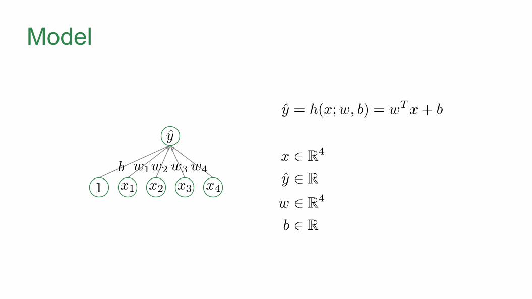
Model

Model

Error Function: Squared Error
Prediction Ground truth / target
Has no special meaning except it makes gradients look nicer

Objective Function
… with a single example
… with a set of examples

Objective Function
Solution

Closed Form Solution
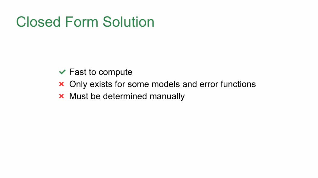
Closed Form Solution
Fast to compute Only exists for some models and error functions Must be determined manually

Gradient Descent

Gradient Descent
1. Initialize at random2. Compute error3. Compute gradients w.r.t. parameters4. Apply the above update rule5. Go back to 2. and repeat until error does not
decrease anymore

Computing Gradients

Computing Gradients
Kronecker delta

Computing Gradients

Computing Gradients

Gradient Descent (Result)
1. Initialize at random2. Compute error3. Compute gradients w.r.t. parameters4. Apply the above update rule5. Go back to 2. and repeat until error does not
decrease anymore
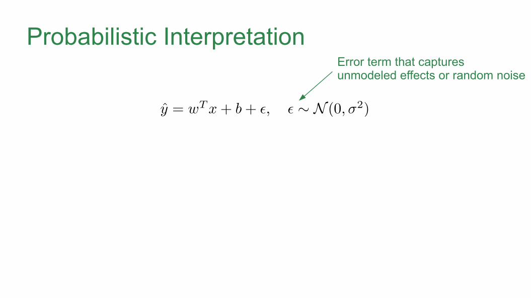
Probabilistic InterpretationError term that captures unmodeled effects or random noise

Probabilistic InterpretationError term that captures unmodeled effects or random noise
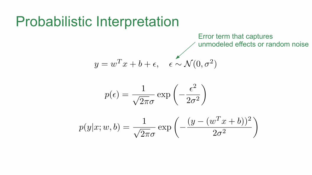
Probabilistic InterpretationError term that captures unmodeled effects or random noise

Likelihood

Maximum Likelihood

Log-Likelihood

Maximum Log-Likelihood
Neural Networks & Backpropagation

Error Function
Prediction Ground truth / target
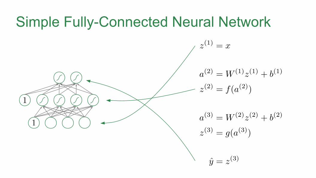
Simple Fully-Connected Neural Network
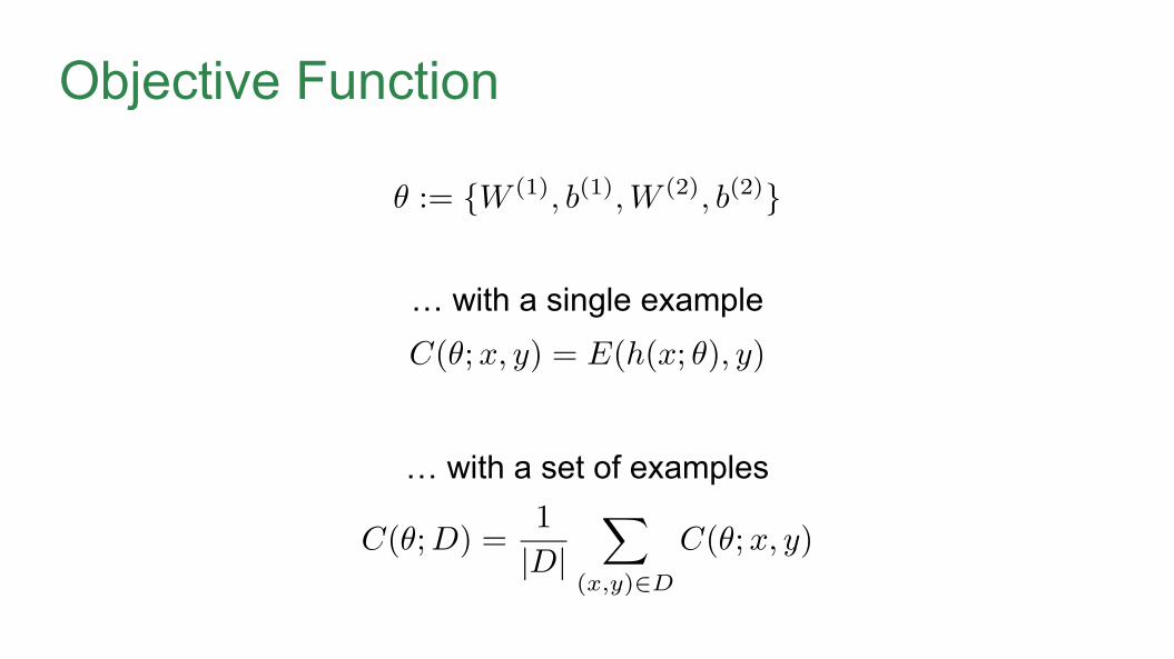
Objective Function
… with a single example
… with a set of examples

Gradients: Towards Backpropagation
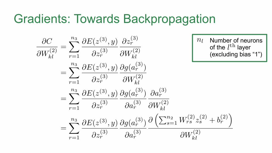
Gradients: Towards Backpropagation
Number of neurons of the layer (excluding bias “1”)

Gradients: Towards Backpropagation
Gradients: Towards Backpropagation
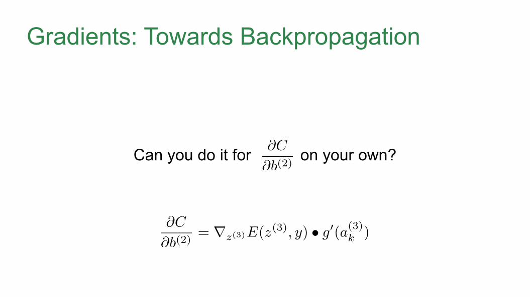
Can you do it for on your own?
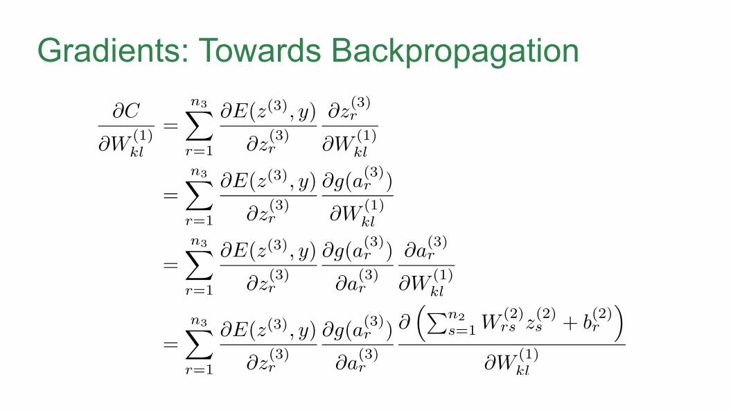
Gradients: Towards Backpropagation

Gradients: Towards Backpropagation

Gradients: Towards Backpropagation

Gradients: Towards Backpropagation

Gradients: Towards Backpropagation

Gradients: Towards Backpropagation
Can you do it for on your own?

Backpropagation
“Delta messages”

Activation Functions
&
Vanishing Gradients

Common Activation Functions

Common Activation FunctionsSmall or even tiny gradient

Vanishing Gradients
Element-wise multiplication with small or even tiny gradients for each layer
In a neural network with many layers, the gradients of the objective function w.r.t. the weights of a layer close to the inputs may become near zero!
⇒ Gradient descent updates will starve

Weight Initialization

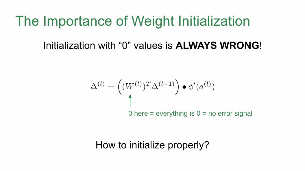
The Importance of Weight Initialization
● Simple CNN trained on MNIST for 12 epochs
● 10-batch rolling average of training loss
Image Source: https://intoli.com/blog/neural-network-initialization/
The Importance of Weight Initialization
Initialization with “0” values is ALWAYS WRONG!
How to initialize properly?
0 here = everything is 0 = no error signal

Information Flow in a Neural Network
Consider a network with ...
● 5 hidden layers and 100 neurons per hidden layer
● the hidden layer activation function = identity function
Let’s omit the bias term for simplicity (commonly initialized with all 0’s).

Information Flow in a Neural Network
Image Source: https://intoli.com/blog/neural-network-initialization/

Information Flow in a Neural Network
What’s the explanation for the previous image?
One layer with some activation function andwithout the bias term:

Information Flow in a Neural Network

Information Flow in a Neural Network
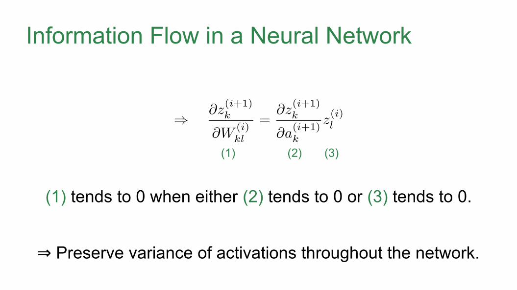
Information Flow in a Neural Network
(1) tends to 0 when either (2) tends to 0 or (3) tends to 0.
⇒ Preserve variance of activations throughout the network.
(1) (2) (3)
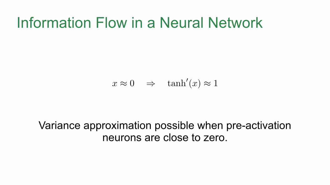
Information Flow in a Neural Network
Variance approximation possible when pre-activationneurons are close to zero.

Variance
Basic properties of variance for independent random variables with expected value = 0

Variance of Activations
Random variables

Variance of Activations
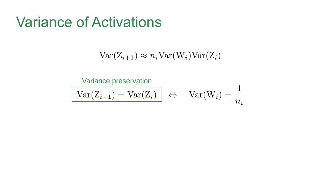
Variance of Activations
Variance preservation

Variance of Error Contribution

Variance of Error Contribution

Variance of Error Contribution
assumption
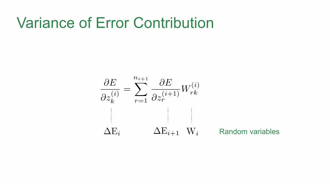
Variance of Error Contribution
Random variables

Variance of Error Contribution

Variance of Error Contribution
Variance preservation
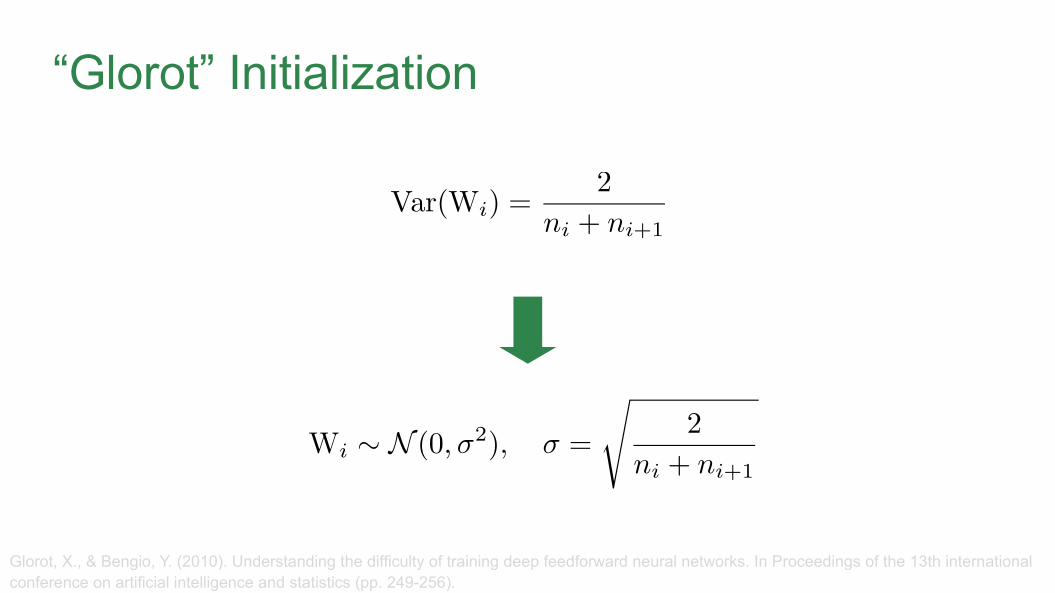
“Glorot” Initialization
Glorot, X., & Bengio, Y. (2010). Understanding the difficulty of training deep feedforward neural networks. In Proceedings of the 13th international conference on artificial intelligence and statistics (pp. 249-256).

Optimization Methods

Gradient Descent
Martens, J. (2010). Deep Learning via Hessian-Free Optimization. In Proceedings of the 27th International Conference on Machine Learning (pp. 735-742).
Too large learning rate ⇒ zig-zag
Too small learning rate ⇒ starvation

Batch Gradient Descent
● Update based on the entire training data set● Susceptible to converging to local minima● Expensive and inefficient for large training data sets

Stochastic Gradient Descent (SGD)
● Update based on a single example● More robust against local minima● Noisy updates ⇒ small learning rate

Mini-Batch Gradient Descent
● Update based on multiple examples● More robust against local minima● More stable than stochastic gradient descent● Most common● Often also called SGD despite multiple examples

Gradient Descent with Momentum
● Momentum dampens oscillations● Gradient is computed before momentum is applied● Typical momentum term:
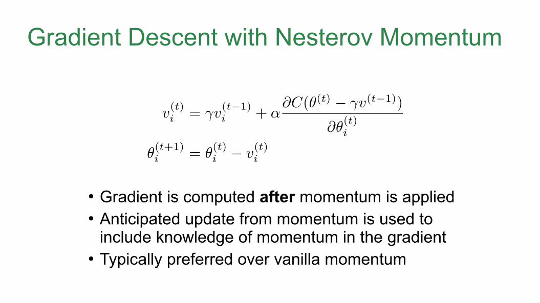
Gradient Descent with Nesterov Momentum
● Gradient is computed after momentum is applied● Anticipated update from momentum is used to
include knowledge of momentum in the gradient● Typically preferred over vanilla momentum

AdaGrad
● Adaptive (per-weight) learning rates● Learning rates of frequently occurring features are
reduced while learning rates of infrequent features remain large
● Monotonically decreasing learning rates● Suited for sparse data● Typical learning rate:

RMSProp
Typical hyperparameters:

Adam
● Often used these days● Typical hyperparameters:

Computation Graphs
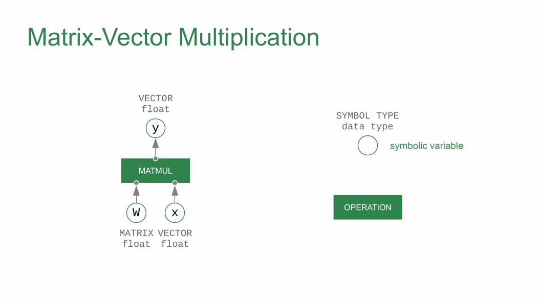
Matrix-Vector Multiplication
MATMUL
W
y
x
MATRIXfloat
VECTORfloat
VECTORfloat
SYMBOL TYPEdata type
OPERATION
symbolic variable

Indexing
INDEXING
A
B
i
MATRIXfloat
VECTORint
MATRIXfloat
2
5
0
A i B
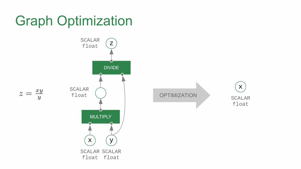
Graph Optimization
MULTIPLY
x
SCALARfloat
SCALARfloat
SCALARfloat
DIVIDE
zSCALARfloat
OPTIMIZATION
x
SCALARfloat
y

Automatic Differentiation
SQUARE
x
y
SCALARfloat
SCALARfloat
GRAD(y, x)
2
SCALARfloat
MULTIPLY
dy/dx
SCALARfloat
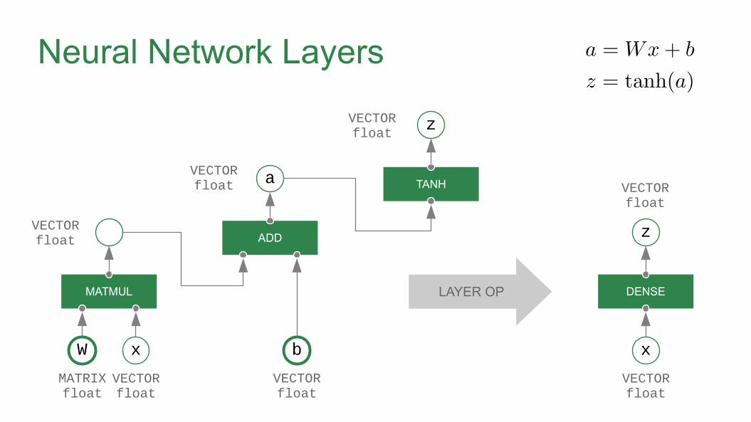
Neural Network Layers
MATMUL
W x
MATRIXfloat
VECTORfloat
VECTORfloat ADD
b
VECTORfloat
a TANH
z
VECTORfloat
VECTORfloat
LAYER OP DENSE
z
x
VECTORfloat
VECTORfloat