DEEP DIVE CASE STUDY 2 - QUT · Energy Efficiency Education Resources for Engineering Project Companion Guide DEEP DIVE CASE STUDY 2: Heavy Industry Electrical Energy Use and System

Energy Efficiency Education Resources for Engineering Project Companion Guide

DEEP DIVE CASE STUDY 2:

Heavy Industry Electrical Energy Use and System

Design for Energy Efficiency and Sustainability

Companion Guide

Project EEERE: Energy Efficiency Education Resources for Engineering

Consortium Partners:

Project Partners:

http://www.google.com.au/url?sa=t&rct=j&q=&esrc=s&frm=1&source=images&cd=&cad=rja&ved=0CAQQjRw&url=http://data.gov.au/organization/department-of-industry&ei=7OYLU8zhJIS6kgWz94Eo&usg=AFQjCNGGH9GdYFBiOTz774Tdodd-voi9VA&sig2=2eII_LgNz5JDgfNwzHAyiw&bvm=bv.61725948,d.dGI


2

Citation Details

All resources developed for the EEERE project are made available to the public through the Creative

Commons Attributes licence. Accordingly, this document should be cited in the following manner:

H.P.A.P. Jayawardana, D. Robinson, (2014) Deep Dive Case Study 2: Heavy Industry Electrical Energy Use and System

Design for Energy Efficiency and Sustainability – Companion Guide, a guide produced by University of Wollongong for

the Energy Efficiency Education Resources for Engineering (EEERE) Project, led by the Queensland University of

Technology. An initiative of the Australian Government’s Department of Industry, Canberra.

Acknowledgements

The consortium thanks the 40 workshop participants (Brisbane, Sydney and Melbourne) including

stakeholder partners, college members, industry and academic colleagues, who provided their time and

ideas so generously during the stakeholder engagement parts of the project, and to those who have

assisted in reviewing the drafted resources. The consortium thanks our project partners for their

continued commitment to building capacity in delivering sustainable solutions, the federal government

for funding the initiative, and the following individuals for their ongoing support of capacity building in

engineering education: Mr Stuart Richardson, Mr Luiz Ribeiro, Ms Denise Caddy and Mr Nick Jackson. The

authors acknowledge the invaluable inputs made by Dr Cheryl Desha of Queensland University of

Technology for her inputs into this case study and leadership of the consortium of academics

participating in the Energy Efficiency Education Resources for Engineering (EEERE) project.

Project Background

Energy efficiency is widely recognised as the simplest and most cost-effective way to manage rising

energy costs and reduce Australia’s greenhouse gas emissions. Promoting and implementing energy

efficiency measures across multiple sectors requires significant development and advancement of the

knowledge and skills base in Australia. Engineering has been specifically identified as a profession with

opportunities to make substantial contributions to a clean and energy-efficient future. To further enable

skills development in this field, the Department of Industry commissioned a consortium of Australian

universities to collaboratively develop four innovative and highly targeted resources on energy efficiency

assessments, for use within engineering curricula. This includes:

1. Ten short ‘multi-media bite’ videos for each engineering college of Engineers Australia and an

introduction (led by Queensland University of Technology with the University of Adelaide);

2. Ten ‘flat-pack’ supporting teaching and learning notes (led by University of Adelaide with QUT);

3. Two ‘deep-dive case studies’ including worked calculations (led by University of Wollongong); and

4. A ‘virtual reality experience’in an energy efficiency assessment (led by Victoria University).

Specifically, these resources address the graduate attributes of ‘identifying’, ‘evaluating’ and

‘implementing’ energy efficiency opportunities in the workplace, incorporating a range of common and

discipline specific, technical and enabling (non-technical) knowledge and skill areas.The four resources

were developed with reference to the 2012 Industry Consultation Report and Briefing Note 1 funded by

the Australian Government’s former Department of Resources, Energy and Tourism (RET), and through

further consultation workshops with project partners and industry stakeholders. At these workshops,

participants confirmed the need for urgent capacity building in energy efficiency assessments,

accompanied by clear guidance for any resources developed, to readily incorporate them into existing

courses and programs. Industry also confirmed three key graduate attributes of priority focus for these

education resources, comprising the ability to: think in systems; communicate between and beyond

engineering disciplines; and develop a business case for energy efficiency opportunities.

1 Desha, C. and Hargroves, K. (2012) Report on Engineering Education Consultation 2012, a report and accompanying Briefing Note,

Australian Government Department of Resources, Energy and Tourism, Canberra.

http://eex.gov.au/business-support/energy-efficiency-skills-and-training/engineering-skills-research-reports-and-information/


3

Contents

Citation Details ................................................................................................................................... 2

Acknowledgements ............................................................................................................................ 2

Project Background ............................................................................................................................ 2

1 Overview .................................................................................................................................. 4

2 Benefits you will gain ................................................................................................................ 4

3 The case study task ................................................................................................................... 5

3.1 The design brief ................................................................................................................... 5

3.1.1 Plant energy demand profile ........................................................................................... 6

3.1.2 Design of plant electrical distribution system and load.................................................... 6

3.1.3 Variable speed drive for plant pumping system............................................................... 6

3.2 Task outcomes ..................................................................................................................... 6

3.3 Task outputs ........................................................................................................................ 7

4 Energy usage analysis ............................................................................................................... 7

4.1 How to use the software ...................................................................................................... 8

5 Energy efficient electrical design............................................................................................. 10

5.1 Transformer selection ........................................................................................................ 10

5.1.1 Transformer selection for energy efficiency .................................................................. 10

5.1.2 Calculations for transformer selection .......................................................................... 11

5.2 Cable selection .................................................................................................................. 11

5.2.1 Cable selection for energy efficiency ............................................................................. 12

5.2.2 Calculations for cable selection ..................................................................................... 12

5.3 Lighting selection ............................................................................................................... 13

5.3.1 Lighting selection for energy efficiency ......................................................................... 13

5.3.2 Calculations for luminaire selection .............................................................................. 14

5.4 Motor selection ................................................................................................................. 14

5.4.1 Motor selection for energy efficiency............................................................................ 15

5.4.2 Calculations for motor selection ................................................................................... 16

6 Variable speed drive systems .................................................................................................. 16

6.1.1 Variable speed drives for energy efficiency ................................................................... 16

6.1.2 Calculations for variable speed drive application........................................................... 18


4

1 Overview

Australia generates about 1.5% of global greenhouse gas emissions. However, on a per capita basis,

Australia is one of the world’s largest polluters2. It is reported that 38% of Australia’s total

greenhouse gas emissions are a result of electrical energy production and industrial processes3.

Reduction in electricity use across all sectors, including heavy industry, and an increase in cleaner

energy production via renewables, is essential for a timely reduction in global energy related

emissions and the promotion of environmental sustainability. Significant reduction in electricity use

in industrial plants can be achieved through increased energy efficiency knowledge and

implemented measures in electricity distribution and plant design.

This document is the Companion Guide to a Deep Dive Case Study analysing energy efficiency in

heavy industry, focusing on electricity distribution and utilisation. This Deep Dive Case Study focuses

on providing knowledge of energy efficiency management strategies and technological options for

improving electrical energy utilisation. The case study provides an overview of energy use within a

typical industrial plant, allows the student to develop an understanding of the energy loss

mechanisms, and enables them to improve their understanding of the impact of design decisions

and equipment selection on overall energy efficiency.

This Deep Dive Case Study will utilise a whole system approach to analysing a heavy industry plant

and electrical distribution system in order to illustrate energy efficiency principals during the design

process. The Deep Dive Case Study will provide the energy requirements for various mechanical and

process loads, identifying how to reduce energy consumption and optimise the design of loads such

as motor and lighting systems. It will also illustrate how to use life cycle cost analysis to determine

the optimal system component rating and type, under the given design conditions, in order to

achieve increased energy efficiency.

2 Benefits you will gain

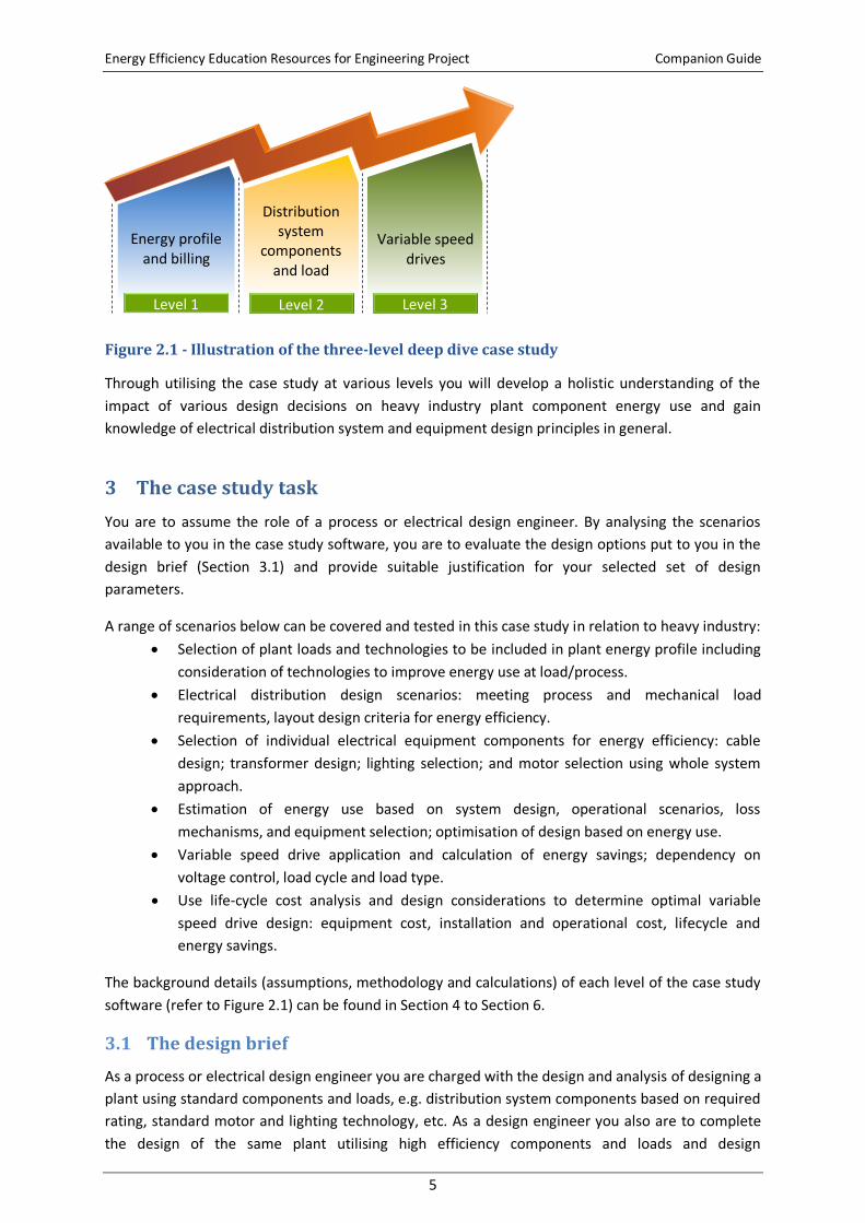
The case study was developed with three different levels of technical details, knowledge and skills,

as illustrated in Figure 2.1. Level 1 focuses on energy use analysis and billing. Based on a base set of

typical industrial loads and design conditions, the students can act as an engineering designer to

estimate the energy use profile of an industrial plant including components such as lighting, air-

conditioning, information technology, plant motors, etc. The students can also evaluate the impact

of modifying time of use of equipment and understand the impact on overall energy use and peak

load. This level allows for discussion on matching load to generation, including the impact of

localised renewable generation, and the cost impact based on flat rate, time of use, or demand

based energy charges.

Level 2 mainly focuses on the energy efficiency and life cycle costs associated with the design of the

electrical supply system. This includes transformer selection, cable sizing and loss calculation, and

lighting and motor type selection. Level 3 focuses on the estimation of energy savings, and impact

on operating cost, for the application of a variable speed drive to a simple pumping system with

variable flow rate requirements. Level 2 and Level 3 use a problem-based learning approach to

highlighting engineering considerations in the design of electrical and pumping systems and

selection of equipment technologies.

2 http://www.carbonneutral.com.au/climate-change/australian-emissions.html, accessed 10th December 2013

3 Commonwealth of Australia, Quarterly Update of Australia’s National Greenhouse Gas Inventory: March 2014,

Department of Environment, http://www.environment.gov.au

http://www.carbonneutral.com.au/climate-change/australian-emissions.html

http://www.environment.gov.au/


5

C

Figure 2.1 - Illustration of the three-level deep dive case study

Through utilising the case study at various levels you will develop a holistic understanding of the

impact of various design decisions on heavy industry plant component energy use and gain

knowledge of electrical distribution system and equipment design principles in general.

3 The case study task

You are to assume the role of a process or electrical design engineer. By analysing the scenarios

available to you in the case study software, you are to evaluate the design options put to you in the

design brief (Section 3.1) and provide suitable justification for your selected set of design

parameters.

A range of scenarios below can be covered and tested in this case study in relation to heavy industry:

Selection of plant loads and technologies to be included in plant energy profile including

consideration of technologies to improve energy use at load/process.

Electrical distribution design scenarios: meeting process and mechanical load

requirements, layout design criteria for energy efficiency.

Selection of individual electrical equipment components for energy efficiency: cable

design; transformer design; lighting selection; and motor selection using whole system

approach.

Estimation of energy use based on system design, operational scenarios, loss

mechanisms, and equipment selection; optimisation of design based on energy use.

Variable speed drive application and calculation of energy savings; dependency on

voltage control, load cycle and load type.

Use life-cycle cost analysis and design considerations to determine optimal variable

speed drive design: equipment cost, installation and operational cost, lifecycle and

energy savings.

The background details (assumptions, methodology and calculations) of each level of the case study

software (refer to Figure 2.1) can be found in Section 4 to Section 6.

3.1 The design brief

As a process or electrical design engineer you are charged with the design and analysis of designing a

plant using standard components and loads, e.g. distribution system components based on required

rating, standard motor and lighting technology, etc. As a design engineer you also are to complete

the design of the same plant utilising high efficiency components and loads and design

Level 1

Energy profile and billing

Level 2

Distribution system

components and load

Level 3

Variable speed drives


6

methodologies aligning with energy efficient practises. You are to complete a full life cycle analysis

of cost of ownership of each plant design, establish energy requirements and quantify emissions.

You are to complete the activities outlined below related to the design of the plants. Assistance in

defining the detailed scope of the task related to the two plant designs will be provided through

workshop discussion.

3.1.1 Plant energy demand profile

By selecting all relevant loads and establishing their time of use, or duty cycle, develop a demand

profile for each equipment type and establish the total plant demand. Analyse how the plant

demand can be manipulated by altering processes in order to produce different plant profiles. By

applying the available billing system options, determine which plant profile provides the least cost

option for each billing type.

3.1.2 Design of plant electrical distribution system and load

For the plant equipment established in Level 1 spreadsheet, design a suitably rated electrical

distribution system based on required ratings only. Establish the energy profile using standing

equipment, e.g. use the least efficient motor and lighting systems. Determine an alternative design

by selecting more energy efficient equipment technologies for motor and lighting, also utilise a more

efficient power system transformer and optimise cable sizing for energy efficiency. Quantify the

difference in up front, operational and life cycle costs of the more efficient plant.

3.1.3 Variable speed drive for plant pumping system

Given that a number of the motor systems in a heavy industrial plant will be related to pumping,

assign a number of the motors in your demand profile from Level 2 spreadsheet to be considered for

variable speed drive applications. Assume that the assigned pumps are throttle controlled in the low

efficiency plant design. Establish the life cycle cost benefit of making those throttle controlled

pumping systems variable speed drive applications.

3.2 Task outcomes

On completing this task, you will have gained knowledge on energy usage analysis and energy

efficient electrical design constraints for heavy industry plants, and established the impact of various

energy efficiency design principles in general.

In the area of plant energy use analysis the key learning activities are as follows:

Understand how each load contributes to create the total demand curve and how control of

loads can bring down the peak demand value;

Understand the effects of a range of variables and equipment selection options (e.g. ratings,

system losses, duty cycle and time of use, etc.) on plant energy use; and

Understand how to optimise the electrical distribution system design in order to reduce

energy consumption and energy costs (including application of different tariff schemes);

Energy efficient Electrical Design:

Understand the effects of a range of variables (e.g. duty cycle, peak demand) have on the

design and selection of electrical distribution system components;

Understand how to determine economic factors such as net present value and return on

investment for justification of energy efficiency projects;

Understand how to appropriately selection power system components, e.g. transformer and

cabling, in order to optimise design for energy efficiency and reduced life cycle costs; and


7

Compare the performance of lighting and electrical motor system under different design

options and energy efficiency retrofit applications.

In the area of variable speed drive design, the key learning activities are as follows:

Understand the effects of a range of variables (e.g. motor rating, process flow requirements,

motor speed) on energy losses in a flow control process;

Understand how to appropriately size pumping system components based on given design

flow rate and system pressure drop calculations;

Understand how to optimise control methods for energy efficiency;

Compare energy losses of electronic variable speed drive controlled systems with valve

controlled pumping systems; and

Understand how variable speed drive applications enable energy efficiency improvements.

3.3 Task outputs

The deliverable output of this task is to be a summary report (limited to six pages) which details the

considerations and design options outlined in the design brief. Specific outputs generated from case

study calculations are to be included in the report to justify design parameter selections and/or

verify impact of design alternatives (where applicable). Discussion and/or recommendations for

optimal plant component and equipment design with respect to the low and high efficiency plant

are to be included in the summary report. Include any external factors (beyond the case study

software options) which you think would be important in regards to minimising plant energy use.

Where activities are undertaken in a group, the summary report must indicate the contributions

from each member. Presentation of results will be required during tutorial discussion.

4 Energy usage analysis

This section is focused on providing knowledge on how each load of a heavy industrial plant impacts

on the overall electrical energy demand, how it contributes to the total annual energy usage, and

how the time of operation impacts on plant peak demand. Users can study various demand curves

related to the different types of loads and compare to the total demand curve. Also, this section

provides an understanding of how the total demand curve changes when the usage percentage

values (time of use and duty cycle) change during a day. Furthermore, in this section the user can

understand how different types of tariff schemes work and establish their selection impacts on

overall operational costs.

The following default loads, listed below, are considered for the initial calculations. The user can

manipulate all these load types and provide additional loads where required. The ranges of

equipment loads are not limited but may be introduced as part of the Deep Dive Case Study task.

Lighting Loads 50 kVA

HVAC loads 50 kVA

Lifts 20 kVA

Computer Loads 75 kVA

Other Loads 50 kVA

Motor loads 20, 2.2 kW

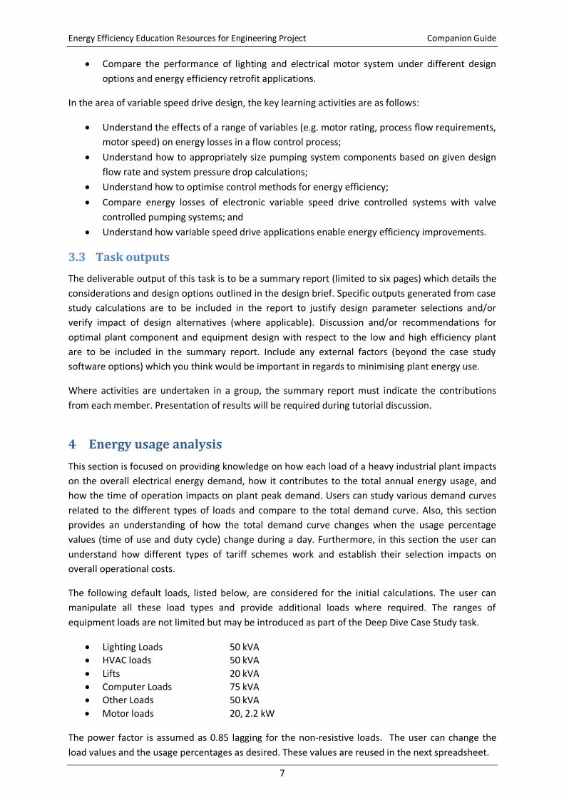
The power factor is assumed as 0.85 lagging for the non-resistive loads. The user can change the

load values and the usage percentages as desired. These values are reused in the next spreadsheet.


8

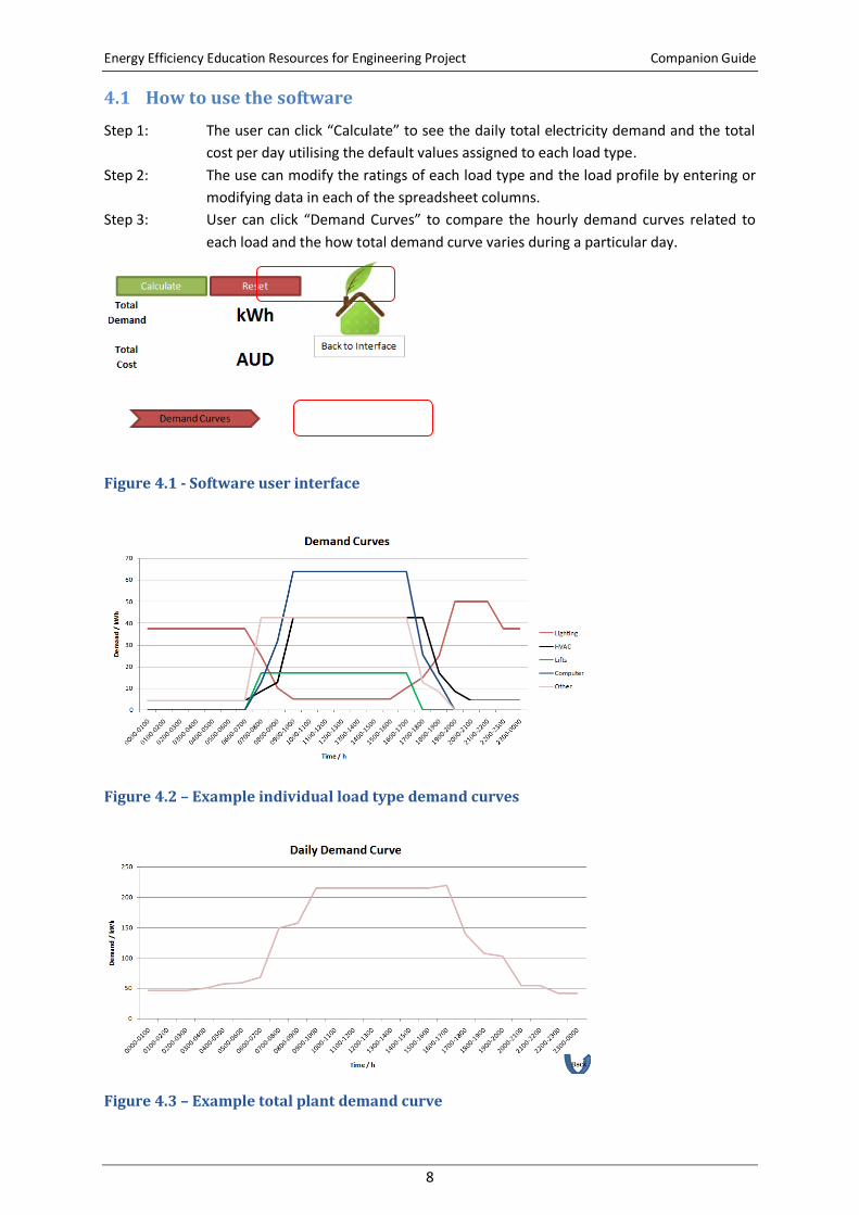
4.1 How to use the software

Step 1: The user can click “Calculate” to see the daily total electricity demand and the total

cost per day utilising the default values assigned to each load type.

Step 2: The use can modify the ratings of each load type and the load profile by entering or

modifying data in each of the spreadsheet columns.

Step 3: User can click “Demand Curves” to compare the hourly demand curves related to

each load and the how total demand curve varies during a particular day.

Figure 4.1 - Software user interface

Figure 4.2 – Example individual load type demand curves

Figure 4.3 – Example total plant demand curve


9

Examples of the graphical output for the individual hourly energy load profiles and total hourly

energy demand curve are illustrated in Figure 4.2 and Figure 4.3.

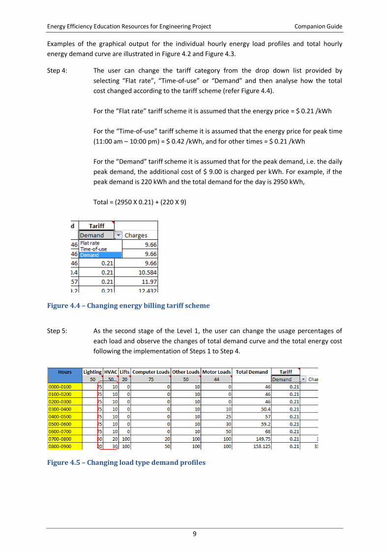
Step 4: The user can change the tariff category from the drop down list provided by

selecting “Flat rate”, “Time-of-use” or “Demand” and then analyse how the total

cost changed according to the tariff scheme (refer Figure 4.4).

For the “Flat rate” tariff scheme it is assumed that the energy price = $ 0.21 /kWh

For the “Time-of-use” tariff scheme it is assumed that the energy price for peak time

(11:00 am – 10:00 pm) = $ 0.42 /kWh, and for other times = $ 0.21 /kWh

For the “Demand” tariff scheme it is assumed that for the peak demand, i.e. the daily

peak demand, the additional cost of $ 9.00 is charged per kWh. For example, if the

peak demand is 220 kWh and the total demand for the day is 2950 kWh,

Total = (2950 X 0.21) + (220 X 9)

Figure 4.4 – Changing energy billing tariff scheme

Step 5: As the second stage of the Level 1, the user can change the usage percentages of

each load and observe the changes of total demand curve and the total energy cost

following the implementation of Steps 1 to Step 4.

Figure 4.5 – Changing load type demand profiles


10

5 Energy efficient electrical design

In the Level 2 spreadsheet of the software, the user can gain knowledge on incorporating energy

efficiency criteria into the design and selection of the major components of a heavy industry

electrical distribution system. For this task, the theory of life cycle costing is used to identify the

present values of the savings from the components of the system. Transformer, cables, lighting

types and motors are considered as the default major components in the system. For each major

component, detailed analysis is provided to assist the user in selection the optimal energy efficient

components.

Data from the Level 1 (energy usage analysis) is used as the default values for this level but may be

altered as required to suit activities.

5.1 Transformer selection

For the energy efficient electrical design (Level 2) spreadsheet within the software the user can

select a suitable rating for the distribution transformer based on system load, standard sizing or by

optimising for energy efficiency. The desired loading of the distribution transformer is selected, a

percentage value can be entered, and by clicking “Calculate” the total load data from the Level 1

spreadsheet is imported into the Level 2 spreadsheet and displayed accordingly. Refer to Figure 5.1.

Then, by comparing with total load, the user can select an appropriate transformer rating (in kVA)

from a drop down list.

Figure 5.1 – Interfacing for Level 2 software platform

5.1.1 Transformer selection for energy efficiency

In this analysis, a standard transformer and a high efficient transformer are compared with their

purchase value, load and no-load losses and derived values for the total owning costs and the

relevant savings.

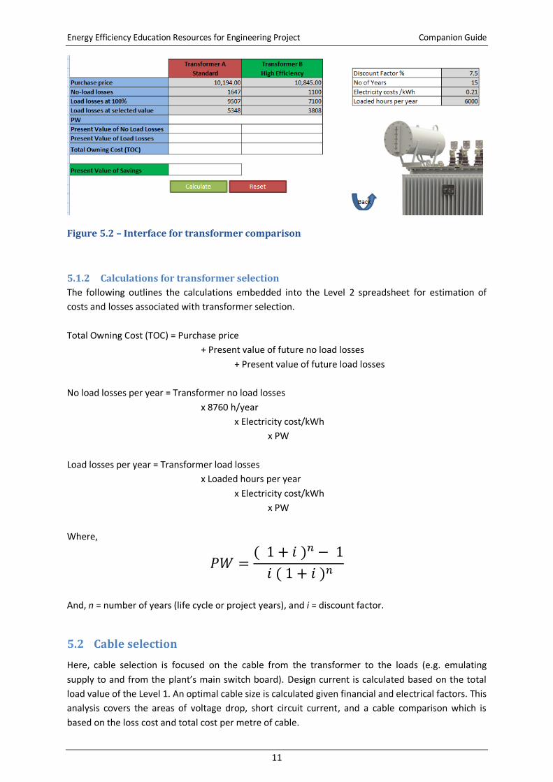
Step 1: Click “Calculate” to see the savings values.

Step 2: Change the loaded hours per year, life cycle of transformer (i.e. number of years),

and determine how the transformer losses and total owning cost change for various

scenarios.


11

Figure 5.2 – Interface for transformer comparison

5.1.2 Calculations for transformer selection

The following outlines the calculations embedded into the Level 2 spreadsheet for estimation of

costs and losses associated with transformer selection.

Total Owning Cost (TOC) = Purchase price

+ Present value of future no load losses

+ Present value of future load losses

No load losses per year = Transformer no load losses

x 8760 h/year

x Electricity cost/kWh

x PW

Load losses per year = Transformer load losses

x Loaded hours per year

x Electricity cost/kWh

x PW

Where,

𝑃𝑊 =( 1 + 𝑖 )𝑛 − 1

𝑖 ( 1 + 𝑖 )𝑛

And, n = number of years (life cycle or project years), and i = discount factor.

5.2 Cable selection

Here, cable selection is focused on the cable from the transformer to the loads (e.g. emulating

supply to and from the plant’s main switch board). Design current is calculated based on the total

load value of the Level 1. An optimal cable size is calculated given financial and electrical factors. This

analysis covers the areas of voltage drop, short circuit current, and a cable comparison which is

based on the loss cost and total cost per metre of cable.


12

5.2.1 Cable selection for energy efficiency

In this analysis, a design using standard cable sizing and a design considering energy efficiency

parameters are completed.

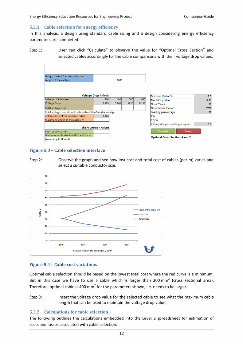
Step 1: User can click “Calculate” to observe the value for “Optimal Cross Section” and

selected cables accordingly for the cable comparisons with their voltage drop values.

Figure 5.3 – Cable selection interface

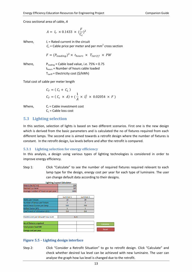
Step 2: Observe the graph and see how lost cost and total cost of cables (per m) varies and select a suitable conductor size.

Figure 5.4 – Cable cost variations

Optimal cable selection should be based on the lowest total cost where the red curve is a minimum.

But in this case we have to use a cable which is larger than 300 mm2 (cross sectional area).

Therefore, optimal cable is 400 mm2 for the parameters shown, i.e. needs to be larger.

Step 3: Insert the voltage drop value for the selected cable to see what the maximum cable length that can be used to maintain the voltage drop value.

5.2.2 Calculations for cable selection


costs and losses associated with cable selection.


13

Cross sectional area of cable, A

𝐴 = 𝐼𝑟 × 0.1433 × (𝐹

𝐶𝑐)2

Where, Ir = Rated current in the circuit Cc = Cable price per meter and per mm2 cross section

𝐹 = (𝑃𝑙𝑜𝑎𝑑𝑖𝑛𝑔)2 × 𝑡ℎ𝑜𝑢𝑟𝑠 × 𝑇𝑡𝑎𝑟𝑖𝑓𝑓 × 𝑃𝑊

Where, Ploading = Cable load value, i.e. 75% = 0.75 thours = Number of hours cable loaded

Ttariff = Electricity cost ($/kWh)

Total cost of cable per meter length

𝐶𝑇 = ( 𝐶𝐼 + 𝐶𝐿 )

𝐶𝑇 = ( 𝐶𝑐 × 𝐴) + ( 1

𝐴 × 𝐼𝑟

2 × 0.02054 × 𝐹 )

Where, CI = Cable investment cost CL = Cable loss cost

5.3 Lighting selection

In this section, selection of lights is based on two different scenarios. First one is the new design

which is derived from the basic parameters and is calculated the no of fixtures required from each

different lamps. The second one is aimed towards a retrofit design where the number of fixtures is

constant. In the retrofit design, lux levels before and after the retrofit is compared.

5.3.1 Lighting selection for energy efficiency

In this analysis, a design using various types of lighting technologies is considered in order to

improve energy efficiency.

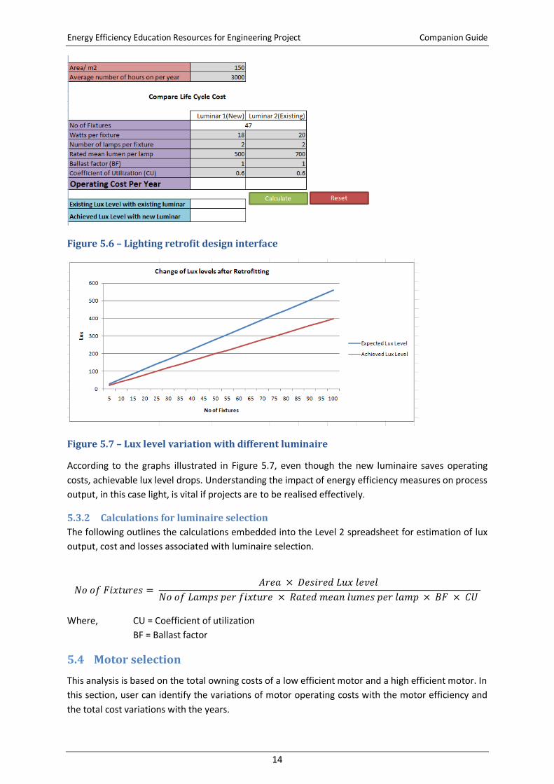
Step 1: Click “Calculate” to see the number of required fixtures required relevant to each

lamp type for the design, energy cost per year for each type of luminaire. The user

can change default data according to their designs.

Figure 5.5 – Lighting design interface

Step 2: Click “Consider a Retrofit Situation” to go to retrofit design. Click “Calculate” and

check whether desired lux level can be achieved with new luminaire. The user can

analyse the graph how lux level is changed due to the retrofit.


14

Figure 5.6 – Lighting retrofit design interface

Figure 5.7 – Lux level variation with different luminaire

According to the graphs illustrated in Figure 5.7, even though the new luminaire saves operating

costs, achievable lux level drops. Understanding the impact of energy efficiency measures on process

output, in this case light, is vital if projects are to be realised effectively.

5.3.2 Calculations for luminaire selection

The following outlines the calculations embedded into the Level 2 spreadsheet for estimation of lux

output, cost and losses associated with luminaire selection.

𝑁𝑜 𝑜𝑓 𝐹𝑖𝑥𝑡𝑢𝑟𝑒𝑠 = 𝐴𝑟𝑒𝑎 × 𝐷𝑒𝑠𝑖𝑟𝑒𝑑 𝐿𝑢𝑥 𝑙𝑒𝑣𝑒𝑙

𝑁𝑜 𝑜𝑓 𝐿𝑎𝑚𝑝𝑠 𝑝𝑒𝑟 𝑓𝑖𝑥𝑡𝑢𝑟𝑒 × 𝑅𝑎𝑡𝑒𝑑 𝑚𝑒𝑎𝑛 𝑙𝑢𝑚𝑒𝑠 𝑝𝑒𝑟 𝑙𝑎𝑚𝑝 × 𝐵𝐹 × 𝐶𝑈

Where, CU = Coefficient of utilization

BF = Ballast factor

5.4 Motor selection

This analysis is based on the total owning costs of a low efficient motor and a high efficient motor. In

this section, user can identify the variations of motor operating costs with the motor efficiency and

the total cost variations with the years.


15

5.4.1 Motor selection for energy efficiency

In this analysis, a design using various types of motor efficiencies is considered in order to improve

overall plant energy efficiency.

Step 1: User can click “Calculate” to compare total owning costs, simple payback periods

and operating costs of motors with different efficiencies. User can change the

efficiency values and related motor cost to see how total owning cost changes.

Figure 5.8 – Motor comparison interface

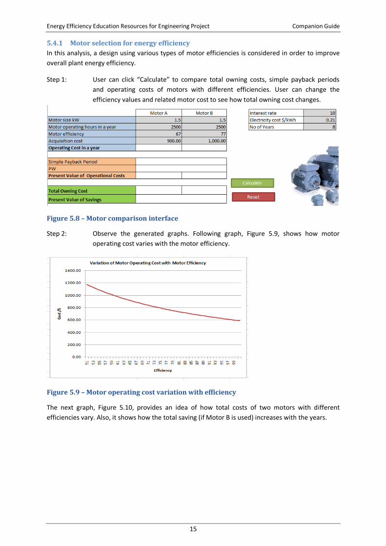
Step 2: Observe the generated graphs. Following graph, Figure 5.9, shows how motor

operating cost varies with the motor efficiency.

Figure 5.9 – Motor operating cost variation with efficiency

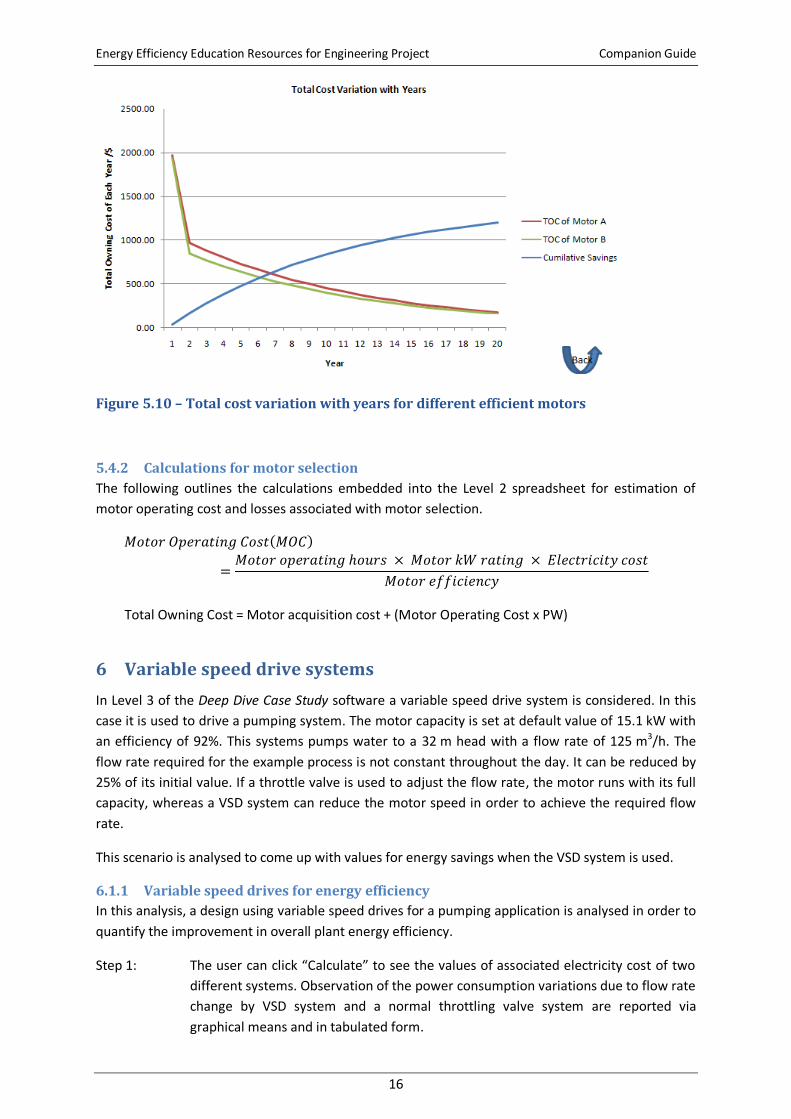
The next graph, Figure 5.10, provides an idea of how total costs of two motors with different

efficiencies vary. Also, it shows how the total saving (if Motor B is used) increases with the years.


16

Figure 5.10 – Total cost variation with years for different efficient motors

5.4.2 Calculations for motor selection


motor operating cost and losses associated with motor selection.

𝑀𝑜𝑡𝑜𝑟 𝑂𝑝𝑒𝑟𝑎𝑡𝑖𝑛𝑔 𝐶𝑜𝑠𝑡(𝑀𝑂𝐶)

=𝑀𝑜𝑡𝑜𝑟 𝑜𝑝𝑒𝑟𝑎𝑡𝑖𝑛𝑔 ℎ𝑜𝑢𝑟𝑠 × 𝑀𝑜𝑡𝑜𝑟 𝑘𝑊 𝑟𝑎𝑡𝑖𝑛𝑔 × 𝐸𝑙𝑒𝑐𝑡𝑟𝑖𝑐𝑖𝑡𝑦 𝑐𝑜𝑠𝑡

𝑀𝑜𝑡𝑜𝑟 𝑒𝑓𝑓𝑖𝑐𝑖𝑒𝑛𝑐𝑦

Total Owning Cost = Motor acquisition cost + (Motor Operating Cost x PW)

6 Variable speed drive systems

In Level 3 of the Deep Dive Case Study software a variable speed drive system is considered. In this

case it is used to drive a pumping system. The motor capacity is set at default value of 15.1 kW with

an efficiency of 92%. This systems pumps water to a 32 m head with a flow rate of 125 m3/h. The

flow rate required for the example process is not constant throughout the day. It can be reduced by

25% of its initial value. If a throttle valve is used to adjust the flow rate, the motor runs with its full

capacity, whereas a VSD system can reduce the motor speed in order to achieve the required flow

rate.

This scenario is analysed to come up with values for energy savings when the VSD system is used.

6.1.1 Variable speed drives for energy efficiency

In this analysis, a design using variable speed drives for a pumping application is analysed in order to

quantify the improvement in overall plant energy efficiency.

Step 1: The user can click “Calculate” to see the values of associated electricity cost of two

different systems. Observation of the power consumption variations due to flow rate

change by VSD system and a normal throttling valve system are reported via

graphical means and in tabulated form.


17

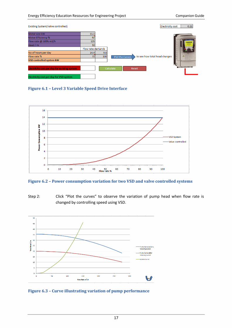
Figure 6.1 – Level 3 Variable Speed Drive Interface

Figure 6.2 – Power consumption variation for two VSD and valve controlled systems

Step 2: Click “Plot the curves” to observe the variation of pump head when flow rate is

changed by controlling speed using VSD.

Figure 6.3 – Curve illustrating variation of pump performance


18

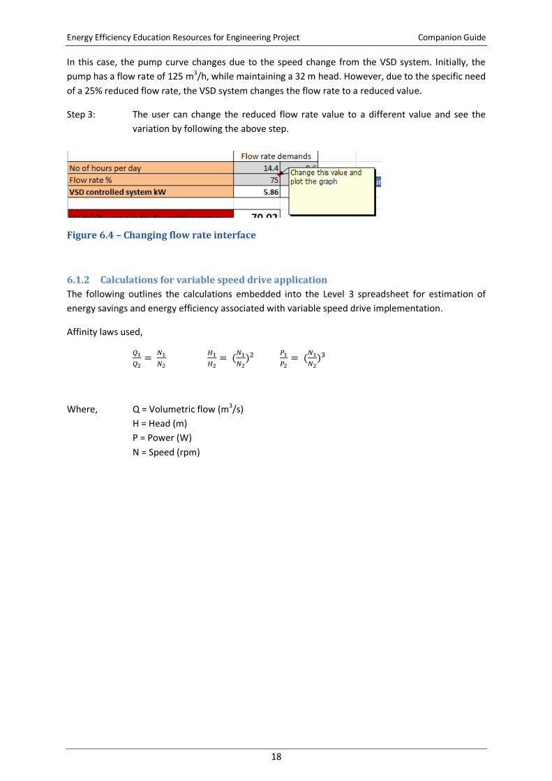
In this case, the pump curve changes due to the speed change from the VSD system. Initially, the

pump has a flow rate of 125 m3/h, while maintaining a 32 m head. However, due to the specific need

of a 25% reduced flow rate, the VSD system changes the flow rate to a reduced value.

Step 3: The user can change the reduced flow rate value to a different value and see the

variation by following the above step.

Figure 6.4 – Changing flow rate interface

6.1.2 Calculations for variable speed drive application


energy savings and energy efficiency associated with variable speed drive implementation.

Affinity laws used,

𝑄1

𝑄2=

𝑁1

𝑁2

𝐻1

𝐻2= (

𝑁1

𝑁2)2

𝑃1

𝑃2= (

𝑁1

𝑁2)3

Where, Q = Volumetric flow (m3/s)

H = Head (m)

P = Power (W)

N = Speed (rpm)

Documents

DEEP DIVE CASE STUDY 2 - QUT · Energy Efficiency Education Resources for Engineering Project Companion Guide DEEP DIVE CASE STUDY 2: Heavy Industry Electrical Energy Use and System