Decreasing Inequality Under Latin America's â€œSocial Democratic

Decreasing Inequality Under Latin

America’s “Social Democratic” and

“Populist” Governments:

Is the Difference Real?

Juan A. Montecino

October 2011

Center for Economic and Policy Research

1611 Connecticut Avenue, NW, Suite 400

Washington, D.C. 20009

202-293-5380

www.cepr.net

CEPR Decreasing Inequality Under Latin America’s “Social Democratic” and “Populist” Governments

i

Contents

Executive Summary ........................................................................................................................................... 1

Introduction ........................................................................................................................................................ 2

A Bit of Background: Good Policies or Good Luck? .................................................................................. 2

Data and Methodology ..................................................................................................................................... 4

Results .................................................................................................................................................................. 6

The Data Source Matters: ECLAC or SEDLAC? ........................................................................................ 9

Conclusion ........................................................................................................................................................ 12

References ......................................................................................................................................................... 13

Appendix ........................................................................................................................................................... 15

Acknowledgements

The author would like to thank John Schmitt and Mark Weisbrot for comments and suggestions, as well as Darryl McLeod for a helpful discussion and for kindly sharing his data.

About the Author

Juan Montecino is a Research Assistant at the Center for Economic and Policy Research in Washington, D.C.

CEPR Decreasing Inequality Under Latin America’s “Social Democratic” and “Populist” Governments 1

Executive Summary This paper addresses the claim that the governments of Argentina, Bolivia, Ecuador and Venezuela, Latin America’s so-called “left-populist” governments, have failed to effectively reduce inequality in the 2000s and have only benefitted from high commodity prices and other benign external conditions. In particular, it examines the econometric evidence presented by McLeod and Lustig (2011) that the “social democratic” governments of Brazil, Chile and Uruguay were more successful and finds that their original results are highly sensitive to which source of data on income inequality is employed. Using data from the Socioeconomic Database for Latin America and the Caribbean (SEDLAC), McLeod and Lustig show that after accounting for favorable external conditions, structural determinants of inequality and the impact of historical and institutional factors, Latin America’s “social democratic” governments appear to have effectively reduced inequality, while the so-called “left-populist” governments have not. However, this paper finds that conducting the same analysis using data on income inequality from the Economic Commission for Latin America and the Caribbean (ECLAC) yields the exact opposite results: it is the so-called “left-populist” governments that appear to have effectively reduced inequality while the “social-democratic” governments have not. The marked contrast between these two results suggests that the choice of sources for data on income inequality is not immaterial and that how SEDLAC and ECLAC handle the underlying household income surveys is the likely culprit. The key difference between data from SEDLAC and ECLAC is that the latter corrects for income underreporting—when households in an income survey underreport their true amount of income, thus biasing the measurement of inequality—while the former does not. Because income underreporting is likely more pronounced in wealthier households, failing to adjust for underreporting is expected to lead to a lower and biased estimate of inequality. However, since the actual pattern of underreporting is unknown, adjusting for underreporting often tends to produce estimates of inequality with an upward bias. Absent reasonable criteria for favoring one source for data on income inequality over the other, this paper suggests that any econometric results should prove robust to both data sources. The paper also examines other issues surrounding McLeod and Lustig’s original approach, including the definitions of the so-called “social democratic” and “left-populist” governments, which are problematic and arguably subjective. Furthermore, the paper also finds econometric evidence that McLeod and Lustig’s original model may be misspecified. These problems, together with the sensitivity to the choice of data source, suggest that McLeod and Lustig’s results should be regarded with a healthy amount of skepticism and that there is no statistical basis to claim that one type of government was more effective at reducing inequality than the other type.


Introduction This paper addresses the claim that the governments of Argentina, Bolivia, Ecuador and Venezuela, Latin America’s so-called “left-populist” governments, have failed to effectively reduce inequality in the 2000s and have only benefitted from high commodity prices and other benign external conditions. In particular, it examines the econometric evidence presented by McLeod and Lustig (2011), who test the effectiveness of Latin America’s leftist regimes at reducing inequality using data on inequality from the Socioeconomic Database for Latin America and the Caribbean (SEDLAC).1 McLeod and Lustig show that after accounting for favorable external conditions, structural determinants of inequality and the impact of historical and institutional factors, Latin America’s “social democratic” governments—Brazil, Chile and Uruguay—appear to have effectively reduced inequality, while the so-called “left-populist” governments have not. This paper attempts to reproduce their findings using data from the Economic Commission for Latin America and the Caribbean (ECLAC). The main result that emerges is that the choice of data source matters tremendously. In fact, conducting the same analysis using data from ECLAC, instead of from SEDLAC, leads to the exact opposite results as those reported by McLeod and Lustig: it is the so-called “left-populist” governments that now appear to have most effectively reduced inequality. The paper proceeds as follows. The first section provides context and a brief summary of the evidence presented by McLeod and Lustig. The second section deals with methodological and data issues. The third presents the results and addresses some relevant econometric issues. The fourth section provides a discussion of the differences between ECLAC and SEDLAC inequality data. The fifth and final section concludes.

A Bit of Background: Good Policies or Good Luck? Latin America has undergone major changes throughout the last two decades. Where once authoritarian regimes of one form or another ruled most of the region, democracy has now become the rule rather than the exception.2 Perhaps more remarkably, beginning around the end of the 1990s, the consolidation of democracy was accompanied by a marked shift to the left of the political spectrum. Starting with the 1998 election of Hugo Chávez in Venezuela, left and center-left governments were repeatedly elected across the region. With the election of Ricardo Lagos in Chile in 2000, Lula da Silva in Brazil in 2002 and then Evo Morales in Bolivia in 2005, by the middle of last decade, the majority of the region was ruled by left of center governments with explicit redistributive platforms.3

1 McLeod and Lustig have presented various versions of this evidence. The current analysis is based on McLeod and

Lustig (2011). The other versions are Lustig and McLeod (2009) and Birdsall, Lustig and McLeod (2011). 2 Of course, the 2009 overthrow of the democratically elected president of Honduras, Mel Zelaya, and the subsequent

and ongoing repression provide a sobering exception to this rule. 3 The other left-of-center governments are the administrations of Nestor Kirchner in Argentina (2003), Tabaré Vázquez

in Uruguay (2005), Rafael Correa in Ecuador (2007), and Fernando Lugo in Paraguay (2008).


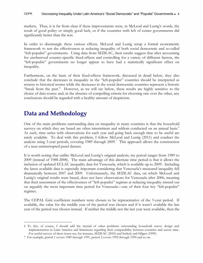
As the number of left-of-center governments increased, however, some scholars and commentators began to distinguish between what they saw as two lefts: a moderate left with respect for property rights and market forces, and an “undemocratic” left rooted in the region’s populist past.4 The former, according to these narratives, is modern, technocratic, and delivers on its promises because of well-designed policies. The latter type, on the other hand, has simply benefitted temporarily from a commodity boom and their policies will eventually prove unsustainable. These changes in the political realm coincided with sustained improvements in social indicators, including significant reductions in inequality in most countries of Latin America.5 Figure 1 compares the levels of inequality, as measured by the Gini coefficient, for the 2007-2009 period and for 2001-2003. The farther a country appears below (above) the 45-degree line, the more it decreased (increased) inequality between the two periods. Thus, as can be seen below, by the end of last decade most countries for which data is available managed to reduce inequality, and in some cases by considerable amounts.

FIGURE 1

Change in Inequality: 2007-09 vs. 2001-03 (Gini Coefficient)

Source: The Economic Commission for Latin America and the Caribbean.

The causes behind these widespread improvements, however, are disputed. As McLeod and Lustig observe, this period was also marked by remarkably benign external conditions, as exemplified, for instance, by favorable terms of trade and bountiful inflows of capital from international financial

4 See Castañeda (2006) for a prominent example of this argument. Another example is, for instance, Vargas Llosa

(2007). 5 For a comprehensive account of social trends in Latin America throughout the last decade see ECLAC (2010).

Gasparini and Lustig (2011) provide an overview of trends in inequality.


markets. Thus, it is far from clear if these improvements were, in McLeod and Lustig’s words, the result of good policy or simply good luck, or if the countries with left of center governments did significantly better than the rest. In order to disentangle these various effects, McLeod and Lustig setup a formal econometric framework to test the effectiveness at reducing inequality of both social democratic and so-called “left-populist” governments. Using data from SEDLAC, their results suggest that after accounting for unobserved country-specific fixed-effects and controlling for a variety of different factors, the “left-populist” governments no longer appear to have had a statistically significant effect on inequality. Furthermore, on the basis of their fixed-effects framework, discussed in detail below, they also conclude that the decreases in inequality in the “left-populist” countries should be interpreted as returns to historical norms while the decreases in the social democratic countries represent a historic “break from the past.” However, as we will see below, these results are highly sensitive to the choice of data source and, in the absence of compelling criteria for choosing one over the other, any conclusions should be regarded with a healthy amount of skepticism.

Data and Methodology One of the main problems surrounding data on inequality in many countries is that the household surveys on which they are based are often intermittent and seldom conducted on an annual basis.6 As such, time series with observations for each year and going back enough time to be useful are rarely available. To deal with this problem, I follow McLeod and Lustig (2011) and conduct the analysis using 3-year periods, covering 1989 through 2009.7 This approach allows the construction of a near uninterrupted panel dataset. It is worth noting that unlike McLeod and Lustig’s original analysis, my period ranges from 1989 to 2009 (instead of 1988-2008). The main advantage of this alternate time period is that it allows the inclusion of updated ECLAC inequality data for Venezuela, which is available up to 2009. Including the latest available data is especially important considering that Venezuela’s measured inequality fell dramatically between 2007 and 2009. Unfortunately, the SEDLAC data, on which McLeod and Lustig’s original results were based, does not have observations for Venezuela after 2006, meaning that their assessment of the effectiveness of “left-populist” regimes at reducing inequality missed out on arguably the most important time period for Venezuela—one of their four key “left-populist” regimes. The CEPAL Gini coefficient numbers were chosen to be representative of the 3-year period. If available, the value for the middle year of the period was chosen and if it wasn’t available the last year of the period was chosen instead. If neither the middle nor the last year were available, then the

6 To this, of course, I should add the myriad of other problems surrounding household survey design and

implementation in Latin America and limitations regarding their comparability between countries and across time. For useful surveys of these issues see, for instance, SEDLAC (2010) and Székely and Hilgert (1999).

7 For example, period 1 covers 1989 through 1991, period 2 covers 1992 through 1994 and so on.


first year of the 3-year period was chosen. The rest of the explanatory variables, with the only exception of the political regime variables, are averages over each 3-year period. The main explanatory variables of interest, the cumulative years in power of social democratic and “left-populist” governments, were constructed using McLeod and Lustig’s methodology, which is based on the political regime typology discussed in Kaufman (2007). These variables count the cumulative number of “effective” years in power for each type of leftist government, or in other words, they count each year after the first in office. This captures the idea that any policies implemented by a particular government wouldn’t take effect right away.

TABLE 1

Cumulative Effective Years in Power by Regime Type

Period 4 Period 5 Period 6 Period 7

(1998-2000) (2001-2003) (2004-2006) (2007-2009)

"Left-Populist"

Argentina 0 0 3 6

Bolivia 0 0 0 3

Ecuador 0 0 0 2

Venezuela 1 4 7 10

Social Democratic

Brazil 0 0 3 6

Chile 0 3 6 9

Uruguay 0 0 1 4

Source: Author’s calculations based on McLeod and Lustig (2011) and Kaufman (2007).

Table 1 shows the cumulative years in power of each regime type. Venezuela’s Hugo Chávez became the first of the new left leaders elected in Latin America in December 1998 and assumed power in February 1999. As such, Venezuela receives one effective year in power for the “left-populist” category in period 4, which spans 1998 to 2000. Similarly, under this typology the election of Chile’s Ricardo Lagos in 2000 marks Chile’s turn to the left and the social democratic category registers three cumulative effective years in period 5. It should be mentioned that this typology of Latin American leftist regimes should be considered cautiously. For instance, classifying Chile as social democratic beginning with the election of socialist Ricardo Lagos is problematic and debatable considering the political continuity between his administration and his predecessor’s, Eduardo Frei. Chile’s turn to the left, in other words, could arguably have begun much earlier with the defeat of General Pinochet during the plebiscite of 1988 and the Concertación’s first transitional administration of Patricio Alwyn. Similarly in Brazil, Lula da Silva’s predecessor, Fernando Henrique Cardoso, could also qualify as a social democrat. Following McLeod and Lustig, I run a panel regression with country and time-fixed effects of the form,


where and are the cumulative effective years in power of social democratic and “left-

populist” regimes, respectively, in country i during period t; is a vector of control variables,

described below; is the country-specific intercept or fixed-effect of each country i; are time-

dummies; and is an independent and identically distributed error term. The fixed country effects control for unobserved time invariant differences between countries, while the time-dummies control for unobserved effects that vary across time. The fixed-effects capture the notion that there are deep historical and institutional factors in each country that determine the level of inequality while the latter takes into account the possibility of external shocks influencing inequality across the entire region. To capture the structural impact of the level of development on inequality, the regressions also control for each country’s level of GDP per capita. In order to examine the extent to which the changes in inequality were driven by favorable external conditions, the regressions also include a measure of the terms of trade, as well as the size of merchandise exports as share of GDP and fuel exports as a share of total merchandise trade.

Results Table 2 shows the results of the regression analysis using data from ECLAC instead of from SEDLAC.8 As can be seen in the table, the main results that emerge from the regression analysis is that the so-called “left-populist” regimes appear to have significantly reduced inequality while the social democratic ones did not; and these results are robust across several different specifications. The estimates suggest that after controlling for structural, external and unobserved country-specific factors, “left-populist” governments effectively reduced the Gini coefficient by between 0.47 and 0.65 percentage points per cumulative year in office. The five regressions, shown in columns (1) through (5), match McLeod and Lustig’s original specifications, which are shown in the Appendix. It is worth mentioning that in their original analysis using SEDLAC data, much of the significance of the social democratic regime variables hinged on the exclusion of Uruguay. This is problematic considering that Uruguay is one of only three social democratic governments in the sample. Nevertheless, in order to match their original specifications, Uruguay is excluded from the analysis in the regressions in columns (1) through (4) and is included in the last regression in column (5).

Column (1) shows the results of the regression without the control variables, with the Gini coefficient as a function of only the cumulative years in power of social democratic and “left-populist” regimes and the level of real GDP per capita in purchasing power parity terms. The coefficient on the “left-populist” cumulative years in power variable is negative indicating that “left-populist” governments are associated with reduced inequality; and it is statistically significant at the 5 percent level. Log real GDP per capita is also negative and significant, consistent with the idea that more developed countries tend to have lower structural levels of inequality.

8 Summary statistics are provided in the Appendix.


TABLE 2

Gini Coefficient Regression Resultsa

(1) (2) (3) (4) (5)

VARIABLES ECLAC ECLAC ECLAC ECLAC ECLAC

SD Years in Power

-0.672 -0.758

(0.538) (0.448)

SD Cumulative Years in Power -0.130 -0.218

-0.305

(0.175) (0.167)

(0.217)

LP Years in Power

-0.499 -0.898***

(0.305) (0.291)

LP Cumulative Years in Power -0.472** -0.648***

-0.648***

(0.175) (0.136)

(0.210)

Government Consumption (log % of GDP)

4.348***

4.295*** 4.496***

(1.023)

(1.040) (1.185)

Social Spending (log % of GDP)

-2.577

-2.596 -2.821

(1.772)

(1.856) (1.821)

Log Real GDP per capita (2005 PPP dollars) -7.678* -7.554* -9.261** -10.048** -10.038**

(4.066) (3.670) (3.829) (3.744) (3.749)

Inflation Rate (Average CPI)

0.018

0.029

(0.074)

(0.076)

Log Terms of Trade Index

-2.727 -3.658** -1.301

(2.098) (1.631) (1.646)

Remittances/GDP

-0.219 -0.178 -0.119

(0.178) (0.187) (0.182)

Log Merchandise Exports (% of GDP)

-0.026 -0.335 -0.770

(1.856) (1.829) (1.836)

Fuel Exports (Log Share of Merchandise)

0.479 0.627* 0.532

(0.340) (0.340) (0.312)

Constant 116.8*** 111.2*** 142.3*** 149.7*** 140.1***

(34.995) (32.744) (30.530) (31.766) (33.702)

Observations 103 98 101 96 99

Number of Countries 17 17 17 17 18

Time Dummies? Yes Yes Yes Yes Yes

R-Squared: Within 0.291 0.358 0.304 0.378 0.385

Time Dummies Joint Significance (p > 0) 0.068 0.410 0.055 0.035 0.075

Wooldridge Panel Autocorrelation Test (p > 0) 0.084 0.028 0.046 0.035 0.078

Robust standard errors in parentheses

*** p<0.01, ** p<0.05, * p<0.1

Note: Columns (1) through (5) correspond to columns 1.4 through 1.8 in Table 2, page 19 of McLeod and Lustig

(2011). McLeod and Lustig’s original results are reproduced in full in the Appendix. a/

Following McLeod and Lustig, Uruguay is excluded from the analysis in (1) through (4) and only included in (5).


By contrast, the coefficient on the cumulative years of power for “social democratic” governments is not significant. Thus, the results for this regression, for both of these variables, are the opposite of what McLeod and Lustig found. Following McLeod and Lustig’s specifications, the regression in column (2) introduces controls for the level of government consumption, public social spending and the rate of inflation.9 As can be seen above, “left-populist” regimes now appear to have had an even larger effect on reducing inequality than in the first regression, and are significant at the 1 percent level. The coefficient on social spending as a percent of GDP is negative, as expected, though not statistically significant. Government consumption appears highly regressive and significant at the 1 percent level. It is worth noting that the use of government consumption and social spending as control variables in these regressions is highly questionable, since these are likely to be important channels through which governments that intend to reduce inequality may do so. Although this regression shows government consumption to be regressive, the opposite was found to be true when looking only at “left-populist” governments; and social spending was found to be correlated with reduced inequality for both “social democratic” and “left-populist” governments.10 Columns (3) and (4) show the results from using alternate regime variables and controlling for the terms of trade, remittances, merchandise exports and the fuel share of exports. Instead of the cumulative years in power of each regime type, the alternate regime variables count the number of years in power per period.11 As can be seen above, the alternate regime variable is less robust than the cumulative years in power. While neither the “left-populist” nor the social democratic governments appear significant in regression (3), the results change significantly after controlling for the level of government consumption and social spending in regression (4). The coefficient on the alternate “left-populist” variable is now almost twice as large and more statistically significant than in regression (1). These large differences between (3) and (4) suggest that the alternate regime variables are likely not very reliable and that the cumulative years in power provide a better measure. The regression in column (5) uses the original cumulative years in power variables and controls for the level of real GDP per capita, the rate of inflation, the terms of trade, remittances, merchandise exports as a share of GDP and the fuel share of exports. As can be seen in the table, the coefficient on the “left-populist” variable is significant at the 1 percent level and the same as the estimate in regression (2). The “social democratic” regime variable is not significant, once again reversing the results of McCleod and Lustig. Finally, the control variables meant to capture the impact of external conditions do not appear very robust. As can be seen in the table, the terms of trade variable has the expected negative sign in (3) through (5) but is only significant in (4). Similarly, the variable for the fuel share of merchandise exports appears consistently positive—in line with theories about the so-called “resource curse”—but is only significant in (4) and only at the 10 percent level. Remittances flows and merchandise

9 Because data on social spending in Venezuela was not available for 2009, a two-year average was used for period 7

instead of the regular three-year averages. 10 Author’s calculations. This is in line with McLeod and Lustigs’s earlier results from McLeod and Lustig (2009). 11 For example, the alternate social democratic variable records 3 years in period 7 for Chile, instead of 9 years in the

cumulative variable.


exports as a share of GDP both have the expected negative signs but neither appears statistically significant in any of the specifications. One common problem associated with the analysis of time-series data is the possibility of serial correlation in the error term, when the model’s disturbances are correlated across time. Serial correlation violates the assumption that the model’s disturbances are random and non-correlated with each other, rendering the estimated coefficients inefficient and leading to unreliably lower standard errors in the regression. In other words, if serial correlation is a problem, variables will tend to appear more statistically significant than they actually are and one may be inclined to reject the null hypothesis that the coefficients are significantly different from zero when perhaps one should not. To assess if serial correlation is a problem I use a panel data serial correlation test discussed by Wooldridge (2002) and implemented by Drukker (2003). The test is based on Wooldridge’s insight that if the model does not exhibit serial correlation, then regressing the residuals from a regression of the model’s first difference on the lagged residuals should yield a coefficient of -0.50. As such, the test runs a regression of the model’s first difference and then performs a Wald test to see whether the coefficient on the lagged residuals is significantly different from -0.50. The p-values from the Wooldridge test are shown at the bottom of Table 2. The null hypothesis is that there is no serial correlation. As can be seen, the null hypothesis is rejected at the 10 percent level in regressions (1) and (5), and at the 5 percent level in regressions (2) through (4). This suggests the presence of serial correlation and that the standard errors could be biased. The evidence of serial correlation is surprising considering that the regressions use 3-year periods and could likely indicate that the model is misspecified.12

The Data Source Matters: ECLAC or SEDLAC? It is clearly problematic that such completely different results—reversing the main conclusions of McLeod and Lustig—emerge simply from using different data sources. Such a major discrepancy suggests that—absent a good reason to trust one source over the other—this research should be regarded with a healthy amount of skepticism, and that further research on the underlying differences between SEDLAC and ECLAC data is in order. This is especially the case if one considers the broader political narratives to which these conflicting results can lend themselves.

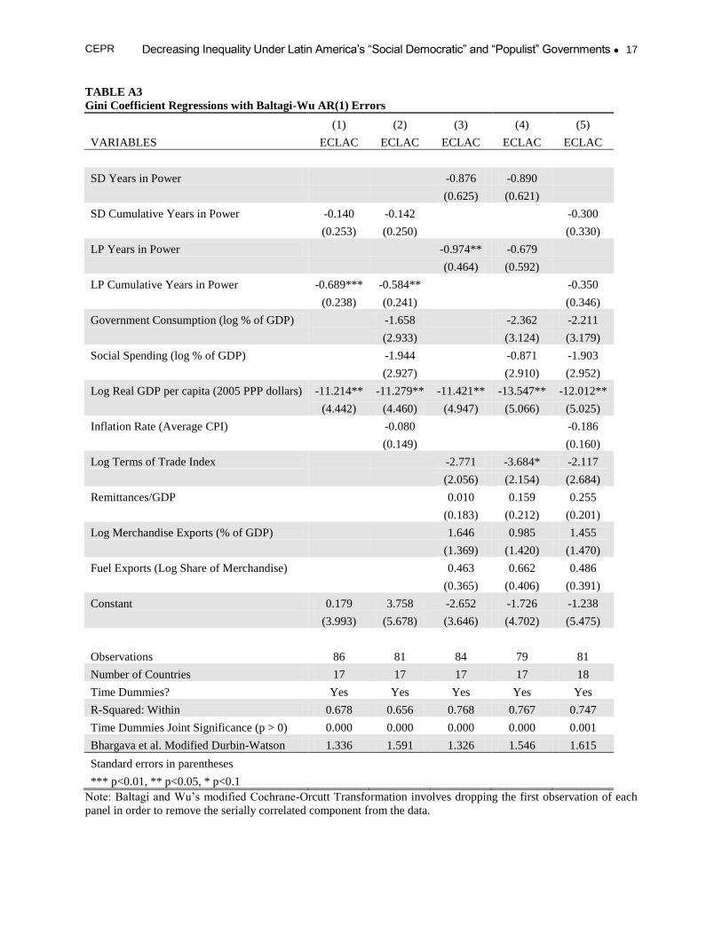
12 It is possible to correct for the presence of serial correlation although it is unclear if this is appropriate if there is

reason to suspect the serial correlation is driven by misspecification. One common way to take it into account is to use fixed-effects regressions with Baltagi-Wu serial correlation-robust (AR(1)) standard errors. The estimation process is based on Baltagi and Wu’s (1999) panel data extension of the Cochrane-Orcutt transformation, which uses

the estimated value of , the serial correlation parameter, to remove the serially correlated component from the data.

The approach estimates by running a Prais-Winsten and Cochrane-Orcutt regression on the demeaned data. Rerunning regressions (1) through (5) with Baltagi-Wu AR(1) errors (see the Appendix) suggests that the main results are not affected significantly by the presence of serial correlation as the “left-populist” regimes are now significant at the 1 percent level in (1) and at the 5 percent level in (2) and (3). However, as expected considering the evidence of serial correlation, the standard errors are larger in all five specifications and the “left-populist” variables lose their significance in (4) and (5).


TABLE 3

Differences Between ECLAC and SEDLAC Gini Coefficients (Percent)

Period 1 Period 2 Period 3 Period 4 Period 5 Period 6 Period 7

(1989-91) (1992-94) (1995-97) (1998-00) (2001-03) (2004-06) (2007-09)

"Left-Populist"

Argentina 7.7 14.4 9.1 10.4 10.7 6.9 11.4

Bolivia .. .. -8.4 -12.5 -7.8 -3.8 -12.8

Ecuador .. .. -17.4 -10.5 -5.9 -4.3 -4.4

Venezuela 10.8 17.7 8.8 6.0 5.3 2.9 ..

Social Democratic

Brazil 0.3 0.8 4.6 6.7 7.0 7.1 8.1

Chile -1.5 -0.5 -0.5 1.1 0.2 -0.2 1.0

Uruguay 16.0 0.5 0.5 0.0 0.2 1.1 -0.2

Source: Author’s calculations based on data from the Economic Commission for Latin America and the Caribbean

and the Socio-economic Database for Latin America and the Caribbean.

As can be seen in Table 3, the Gini coefficients reported by ECLAC in some cases differ from SEDLAC’s by as much as 17 percent. These large differences in measured inequality are all the more surprising considering that both datasets are based on the same underlying official household income surveys. The key difference between the two datasets lies in the handling of the raw surveys. In particular, ECLAC explicitly adjusts the surveys for income underreporting—when households in an income survey underreport their true amount of income, thus biasing the measurement of inequality— while SEDLAC does not.13 Because income underreporting is likely more pronounced in wealthier households, failing to adjust for underreporting is expected to lead to a lower and biased estimate of inequality. However, since the actual pattern of underreporting is unknown, adjusting for underreporting often tends to produce estimates of inequality with an upward bias. 14

The now well-known adjustment process, which was originally outlined by Altimir (1987), is based on reconciling the income reported in the household surveys with macro data from the national accounts. This was motivated by the systematically lower income per capita obtained from household survey data, as compared to the national accounts.15 To give a rough sketch of the process: first, aggregate per capita income by category is obtained from the household survey data and then compared to that derived from the national accounts. Then, based on the gap between the

13 Of course, other methodological differences exist. For instance, ECLAC addresses the problem of income non-

response while SEDLAC does not, although no consensus exists over the proper way to deal with missing observations. See Paraje (2003) for an analysis of the impact of non-response on the measurement of inequality and Helwege and Birch (2007) for an account of the differences between SEDLAC and ECLAC’s handling of household surveys.

14 Székely and Hilgert (1999) provide detailed evidence that Latin American surveys are particularly deficient when it comes to measuring the income of those at the top of the income distribution. For instance, they find that in several countries the average income of the top 10 richest households in the surveys were significantly smaller than the wages of a typical manager of an average Latin American firm, suggesting that the income of the rich is grossly underestimated.

15 See Atkinson and Micklewright (1983) for an early account of this discrepancy for the United Kingdom. Similarly, Atkinson et al (1995) extend this analysis to OECD countries. Altimir (1987) provides a comprehensive survey of these discrepancies in Latin America. Ravallion (2001) systematically examines the discrepancy between survey data and national accounts for a large sample of developing countries.


two, an adjustment factor is derived for each income category. In the final step, the income reported in the surveys is scaled-up by multiplying it by the adjustment factor. One detail about the final step deserves special attention. Altimir argues that it is reasonable to assume that the underreporting of property income is limited to the top quintile of the income distribution. Thus, whereas the adjustment factors are applied to the entire distribution of the other income categories, only the top quintile of reported property incomes receive the adjustment for property income. Despite the importance of this well-known correction process, relatively little has been written on its merits and shortcomings. Several studies have pointed out that the adjustment process may simply replace the bias from underreporting with a new bias from the correction method, but few have tried to systematically quantify the tradeoff or how it affects different inequality indexes.16 A notable exception is Paraje (2003), who employs an experimental approach to quantify the magnitude of the bias introduced by the underreporting of property income and the bias produced by the national accounts-based adjustment method. Using a range of simulated income distributions with varying patterns and degrees of underreporting, Paraje shows that the bias from underreporting in an unadjusted sample is broadly comparable in magnitude to —and in some cases smaller than —the bias from the adjustment process.17 The magnitude of the differences between ECLAC and SEDLAC data wouldn’t matter very much for a fixed-effects approach if these were constant across time because what is important for this type of analysis is the variation within each country. However, the differences between the two data sets appear to fluctuate quite a lot in some countries and in a few cases are most pronounced in the first few observations. Since the fixed-effects approach relies on accounting for unobserved time-invariant factors by allowing country-specific intercepts, the large observed differences between ECLAC and SEDLAC’s data for the first few observations can have large implications and alter the sign and significance of the explanatory variables. To give a concrete example, Venezuela’s initial inequality is much higher according to ECLAC data than according to SEDLAC’s, which contributes to a positive fixed-effect instead of the negative one reported by McLeod and Lustig. This could be interpreted as meaning that the unobserved impact of historical and institutional factors increase inequality in Venezuela according to ECLAC’s data while SEDLAC’s suggests that inequality, in the long-run, should be lower than current levels. Clearly, both cannot simultaneously be true and the difference matters quite a lot when interpreting Venezuela’s experience over the last decade. 16 It is beyond the scope of this paper to provide a full survey of this literature. However, see Lustig and Mitchell

(1995) for early applications of the adjustment process to poverty estimates in Mexico. Helwege and Birch (2007) provide a useful survey of the differences in the handling of income surveys between various international organizations. World Bank (2004) discusses some problems with common underreporting correction methods. Bravo and Valderrama Torres (2011) decompose the effects of the adjustment process by income category for the case of Chile’s Casen surveys.

17 For instance, in one simulation where property income is concentrated in the top 10% of the income distribution and as many as 75% of survey respondents underreport, the underreporting bias leads to an underestimation of the Gini coefficient of between 5.6% and 5.8%. The bias from the correction method, on the other hand, leads to an overestimation of the Gini coefficient of between 2% and 4.3%. Paraje also shows that out of all the most common inequality measures, the Gini coefficient is relatively less sensitive to underreporting adjustments made at both the lower and upper tails of the income distribution.


McLeod and Lustig note that they avoid ECLAC data because its correction for income underreporting is “controversial.” Although relying instead on SEDLAC’s unadjusted data certainly has its appeals and ECLAC’s adjustment method is imperfect, there is nevertheless no clear a priori rationale for discarding an imperfect adjustment in favor of no adjustment at all, especially when the bias due to underreporting is likely at least comparable to the bias introduced by the correction method. Thus, in the absence of compelling criteria for privileging one data set over the other, it is reasonable to suggest that econometric results should be robust to both sources.

Conclusion This paper examined the claim that Latin America’s “social democratic” governments have effectively lowered income inequality in their respective countries through effective policies, while so-called “left-populist” governments have not. It found that using inequality data from ECLAC leads to the exact opposite conclusion: it is the “left-populist” countries (i.e. Argentina, Bolivia, Ecuador and Venezuela) that appear to have effectively lowered income inequality. The original results reported by McLeod and Lustig (2011), thus, appear highly sensitive to the use of data from SEDLAC. It is worth noting that the McLeod and Lustig study is problematic for a whole host of reasons, beginning with the arbitrary and ill-defined nature of the distinction between the two types of government that it is comparing. It is not clear that the distinction captures anything more than a general antipathy toward one group of governments and a more positive attitude toward the other group. As noted above, Chile’s “social democratic” period could just as easily have begun with the first Concertación transitional government in 1989, and Brazil’s with the Cardoso administration of 1995 through 2002. And as also noted, there are econometric indications that their model may be otherwise misspecified. For these reasons, the current study makes no attempt, as McLeod and Lustig do, to draw conclusions about the relative effectiveness of countries classified into these two rather dubious categories, in reducing income inequality. Nor does it argue that one data set, which produces opposite results from the other, is superior to that other data set. Rather, the aim is simply to caution against attempts to draw conclusions with potentially major policy implications when something as fundamental as the choice of dataset so drastically alters the results. Thus, for further cross-country econometric research on the determinants of income inequality in Latin America to be useful, more effort needs to be devoted to systematically understand the differences between the main sources of data on income inequality and the relative biases introduced by their underlying methods. In this context, empirical research on the patterns of income underreporting, both between countries and across time, as well as their impact on the measurement of inequality in Latin America would likely be a fruitful avenue for future research.


References Altimir, Oscar. 1987. “Income Distribution Statistics in Latin America and Their Reliability.” Review of Income and Wealth. Vol. 33, Issue 2, pp. 111-155. Atkinson, Anthony Barnes and John Micklewright. 1983. “On the Reliability of Income Data in the Family Expenditure Survey 1970-1977.” Journal of the Royal Statistical Society. Vol. 146, No. 1, pp. 33-61. Baltagi, Badi H and Ping X. Wu. 1999. “Unequally Spaced Panel Data Regressions With AR(1) Disturbances.” Econometric Theory 15: 814-823 Barro, Robert. 2008. “Inequality and Growth Revisited.” Asian Development Bank. Working Paper Series on Regional Economic Integration. N.11. Birdsall, Nancy, Nora Lustig and Darryl McLeod. 2011. “Declining Inequality in Latin America: Some Economics, Some Politics.” Center for Global Development. Working Paper 251. Bravo, David and Jose A. Valderrama Torres. 2011. “The Impact of Income Adjustment in the Casen Survey on the Measurement of Inequality in Chile.” Universidad de Chile. Estudios de Economía. Vol. 38 – N.1, pp. 43-65. Castañeda, Jorge. 2006. Latin America’s Left Turn. Foreign Affairs. CEDLAS and the World Bank. 2010. “A Guide to the Socioeconomic Database for Latin America and the Caribbean.” CEPAL. 2010. “La hora de la igualdad: brechas por cerrar, caminos por abrir.” Drukker, David M. 2003. “Testing for Serial Correlation in Linear Panel-Data Models.” The Stata Journal 3, Number 2, pp. 168-177. Gasparini, Leonardo and Nora Lustig. 2011. “The Rise and Fall of Inequality in Latin America.” Society for the Study of Economic Inequality. Working Paper Series 2011-213. Helwege, Ann and Melissa Birch. 2007. “Declining Poverty in Latin America? A Critical Analysis of New Estimates by International Institutions.” Global Development and Environment Institute. Working Paper No. 07-02. Kaufman, Robert. 2007. “Political Economy and the ‘New Left.’” The ‘New Left’ and Democratic Governance in Latin America. Edited by Arnson, Cynthia, and José Raúl Perales. Woodrow Wilson International Center for Scholars. Lustig, Nora and Darryl McLeod. 2009. “Are Latin America’s New Left Regimes Reducing Inequality Faster?” Addendum to Poverty, Inequality and the New Left in Latin America. Woodrow Wilson International Center for Scholars. Latin America Program.


Lustig, Nora and Ann Mitchell. 1995. “Poverty in Mexico: The Effects of Adjusting Survey Data for Under-Reporting.” Estudios Económicos. Vol. 10, No. 1 (19), pp. 2-28. McLeod, Darryl and Nora Lustig. 2011. “Inequality and Poverty under Latin America’s New Left Regimes.” Tulane Economics Working Paper Series. Working Paper 1117. Paraje, Guillermo Raul. 2003. “How Does Underreporting Affect Inequality Evaluation? A Simulation Approach.” Three Essays on Inequality Measurement (with a special reference to Argentina). Doctoral Dissertation submitted to the University of Cambridge. Székely, Miguel and Marianne Hilgert. 1999. “What’s Behind the Inequality We Measure: An Investigation Using Latin American Data.” The Inter-American Development Bank. Working Paper #409. Vargas Llosa, Alvaro. 2007. “The Return of the Idiot.” Foreign Policy. Wooldridge, Jefferey M. 2002. Econometric Analysis of Cross Section and Panel Data. Cambridge, MA: MIT Press. World Bank. 2004. “Inequality in Latin America and the Caribbean: Breaking with the Past?”


Appendix TABLE A1

Summary Statistics

Variable Obs. Mean

Std.

Dev. Min

Ma

x

ECLAC Gini Coefficient 110 51.33 4.95 41.2 62.5

SD Cumulative Years in Power 126 0.25 1.20 0 9

SD Regime Years per Period 126 0.15 0.65 0 3

LP Cumulative Years in Power 126 0.30 1.32 0 10

LP Regime Years per Period 126 0.18 0.69 0 3

Government Consumption (log % of GDP) 126 2.43 0.33 1.3 3.4

Social Spending (log % of GDP) 119 2.32 0.48 1.2 3.2

Log Real GDP per capita (2005 PPP

dollars) 126 8.70 0.49 7.5 9.5

Inflation Rate (Average CPI) 126 1.13 5.20 0 37.6

Log Terms of Trade Index 126 4.61 0.17 4.2 5.4

Remittances/GDP 119 3.37 4.43 0 19.8

Log Merchandise Exports (% of GDP) 126 2.88 0.51 1.6 3.9

Fuel Exports (Log Share of Merchandise) 124 1.10 2.12 -5.7 4.6

Number of Countries 18

Number of Periods 7

Source: Author’s calculations. Data for government consumption, real GDP per capita, terms of trade, remittances,

merchandise exports and fuel exports come from the World Bank’s World Development Indicators. Inflation data

came from the IMF’s World Economic Outlook. Social spending as a percent of GDP came from the Economic

Commission for Latin America and the Caribbean.

FIGURE A1

ECLAC vs. SEDLAC Gini Coefficients (1989-2009, 3-year periods)


TABLE A2

Original SEDLAC Gini Coefficient Regressions from McLeod and Lustig (2011)a

a This table was reproduced from Page 19 of McLeod and Lustig (2011).


TABLE A3

Gini Coefficient Regressions with Baltagi-Wu AR(1) Errors

(1) (2) (3) (4) (5)

VARIABLES ECLAC ECLAC ECLAC ECLAC ECLAC

SD Years in Power

-0.876 -0.890

(0.625) (0.621)

SD Cumulative Years in Power -0.140 -0.142

-0.300

(0.253) (0.250)

(0.330)

LP Years in Power

-0.974** -0.679

(0.464) (0.592)

LP Cumulative Years in Power -0.689*** -0.584**

-0.350

(0.238) (0.241)

(0.346)

Government Consumption (log % of GDP)

-1.658

-2.362 -2.211

(2.933)

(3.124) (3.179)

Social Spending (log % of GDP)

-1.944

-0.871 -1.903

(2.927)

(2.910) (2.952)

Log Real GDP per capita (2005 PPP dollars) -11.214** -11.279** -11.421** -13.547** -12.012**

(4.442) (4.460) (4.947) (5.066) (5.025)

Inflation Rate (Average CPI)

-0.080

-0.186

(0.149)

(0.160)

Log Terms of Trade Index

-2.771 -3.684* -2.117

(2.056) (2.154) (2.684)

Remittances/GDP

0.010 0.159 0.255

(0.183) (0.212) (0.201)

Log Merchandise Exports (% of GDP)

1.646 0.985 1.455

(1.369) (1.420) (1.470)

Fuel Exports (Log Share of Merchandise)

0.463 0.662 0.486

(0.365) (0.406) (0.391)

Constant 0.179 3.758 -2.652 -1.726 -1.238

(3.993) (5.678) (3.646) (4.702) (5.475)

Observations 86 81 84 79 81

Number of Countries 17 17 17 17 18

Time Dummies? Yes Yes Yes Yes Yes

R-Squared: Within 0.678 0.656 0.768 0.767 0.747

Time Dummies Joint Significance (p > 0) 0.000 0.000 0.000 0.000 0.001

Bhargava et al. Modified Durbin-Watson 1.336 1.591 1.326 1.546 1.615

Standard errors in parentheses

*** p<0.01, ** p<0.05, * p<0.1

Note: Baltagi and Wu’s modified Cochrane-Orcutt Transformation involves dropping the first observation of each

panel in order to remove the serially correlated component from the data.

Documents

Decreasing Inequality Under Latin America's â€œSocial Democratic