Decoupled and unidirectional asymptotic models for the ... · PDF fileDecoupled and unidirectional asymptotic models for the propagation of internal waves Vincent Duch^ene December

Decoupled and unidirectional asymptotic models for the

propagation of internal waves

Vincent Duchene∗

December 17, 2012

Abstract

We study the relevance of various scalar equations, such as inviscid Burgers’, Korteweg-deVries (KdV), extended KdV, and higher order equations (of Camassa-Holm type), as asymptoticmodels for the propagation of internal waves in a two-fluid system. These scalar evolutionequations may be justified with two approaches. The first method consists in approximatingthe flow with two decoupled, counterpropagating waves, each one satisfying such an equation.One also recovers homologous equations when focusing on a given direction of propagation,and seeking unidirectional approximate solutions. This second justification is more restrictiveas for the admissible initial data, but yields greater accuracy. Additionally, we present severalnew coupled asymptotic models: a Green-Naghdi type model, its simplified version in the so-called Camassa-Holm regime, and a weakly decoupled model. All of the models are rigorouslyjustified in the sense of consistency.

1 Introduction

1.1 Motivation

In this paper, we study asymptotic models for the propagation of internal waves in a two-fluid sys-tem, which consists in two layers of immiscible, homogeneous, ideal, incompressible and irrotationalfluids under the only influence of gravity. We assume that there is no topography (the bottom isflat) and that the surface is confined by a flat rigid lid, although the case of a free surface could behandled with our method. The interface between the two layers of fluids is given as the graph of afunction, ζ(t, x), which expresses the deviation from its rest position (x, z), z = 0 at the spatialcoordinate x and at time t. As we will focus on scalar models, we restrict ourselves to the case ofhorizontal dimension one. The governing equations of such a system, describing the evolution ofthe deformation of the interface, ζ(t, x), as well as the velocity flow inside the two layers of fluid isrecalled in Figure 1 (see Section 2 for more details).

The mathematical theory for this system of equation (the so-called full Euler system) is ex-tremely challenging; see [46] in particular. which has led to extensive works concerning simplified,asymptotic models, aiming at capturing the main characteristics of the flow with much simplerequations, provided the size of given parameters. Relevant dimensionless parameters that may besmall in oceanographic situations include1

ε =a

d1; µ =

d21

λ2;

where ε measures the amplitude of the deformation at the interface with respect to the depth of thelayers of fluids, and µ measures the shallowness of the two layers of fluid, when compared with thetypical wavelength of the deformation. Among other works, we would like to highlight [9], where

∗Department of Applied Physics and Applied Mathematics, Columbia University, New York, U.S.A.1Of course, these two dimensionless parameters describe only part of the many different regimes that may be

considered; see (1.1) for the precise regime we consider in this work. Other relevant regimes are quickly discussedthereafter and we refer to the survey article [33] and references therein for a good overview of the oceanographicsignificance of asymptotic models in our regime.

2 Decoupled and unidirectional asymptotic models for the propagation of internal waves

Figure 1: Sketch of the domain, and full Euler system

many asymptotic models are presented and rigorously justified, in a wide range of regimes. In eachcase, the resulting model consists in two relatively simple evolution equations coupling the shearvelocity and the deformation at the interface.

However, in this work, we are mainly interested in scalar models, which can be used in particular(but not only as we shall see) to describe the unidirectional propagation of gravity waves. Thederivation and study of such models have a very rich and ancient history, starting with the work ofBoussinesq [12] and Korteweg-de Vries [44] which introduced the famous Korteweg-de Vries equation

(KdV) ∂tu + c∂xu + αu∂xu + ν∂3xu = 0,

in the context of propagation of surface gravity waves, above one layer of homogeneous fluid (whichwe refer as “water-wave problem”). However, let us note that the complete rigorous justification ofsuch model is recent: [39, 59, 8]. Such a justification is to be understood in the following sense: inthe long wave regime

ε ∼ µ 1,

the flow can be accurately approximated as a decomposition into two counterpropagating waves,each component satisfying a KdV equation (or more generally, with the same order of accuracy, aBenjamin-Bona-Mahony equation [6, 56]).

(BBM) ∂tu + c∂xu + αu∂xu + νx∂3xu − νt∂2

x∂tu = 0,

The situation is similar in the case of two layers of immiscible fluids, with a rigid lid (as well as inthe case of two layers with a free surface, except the flow is then decomposed into four propagatingwaves), and corresponding results are presented in [25].

Of course the coefficients (c, α, ν, etc.) depend on the situation, and a striking difference be-tween the water-wave case and the case of internal waves is that in the latter case, there exists acritical ratio for the two layers of fluid (depending on the ratio of the mass densities) for whichthe nonlinearity coefficient α vanishes. In that case, heuristic arguments support the inclusion ofthe next order (cubic) nonlinearity, which yields the modified KdV equation (see [54] and referencestherein):

(mKdV) ∂tu + c∂xu + α2u2∂xu + νx∂

3xu − νt∂2

x∂tu = 0.

For the cubic nonlinearity to be of the same order of magnitude as the dispersive terms, this urges toconsider the so-called (refering to [20] for this non-standard denomination) Camassa-Holm regime:

ε2 ∼ µ 1.

Note that this regime is interesting by itself as it allows larger amplitude waves than the long waveregime, and in particular yields models developing finite time breaking wave singularities [19, 20].

Vincent Duchene 3

Thus we ask: Can we extend to the Camassa-Holm regime the rigorous justification of the smallamplitude (long wave) one?

As we shall see, the answer is not straightforward, as several evolution equations are in compe-tition, with an accuracy depending on the situation, and in particular the criticality of the depthratio, and localization in space of the initial data. In addition to the equations already presentedabove, we consider the extended KdV (or Gardner) equation

(eKdV) ∂tu + c∂xu + α1u∂xu + α2u2∂xu + νx∂

3xu − νt∂2

x∂tu = 0,

as presented in [38, 23, 50], studied in [31, 55, 57] (among other works), and tested against experi-ments in [43, 34, 49]. More generally, we work with the higher order model

∂tu + c∂xu + α1u∂xu + α2u2∂xu + α3u

3∂xu + νx∂3xu − νt∂2

x∂tu

+ ∂x(κ1u∂

2xu + κ2(∂xu)2

)= 0.(CL)

Such a model has been presented and justified (in the water-wave setting, and in the Camassa-Holmregime) in [20]; we therefore designate it as Constantin-Lannes equation. This equation is related,though slightly different from the Camassa-Holm equation obtained for example in [14, 37] or higherorder models (see various such models formally derived in [64, 27, 28, 17, 32, 53, 26, 21], concerningthe water wave or internal wave problem). However, each of these works is limited to the restrictiveassumption that only one direction of propagation is non-zero.

We propose to study in detail the justification of the decomposition of the flow (although theunidirectional case is also treated) as presented above, and in the case of internal waves with a rigidlid. Our results are expressed in a very general setting: assuming only

µ 1 and ε 1,

and expressing the accuracy of the different models as a function of these parameters. Although thiscomplicates the expression of our results, and renders the proofs fairly technical, such choice allowsto cover general regimes, including the long-wave as well as the Camassa-Holm regimes, describedabove. We recover in particular the relevance of the KdV approximation in the long wave regime.In the Camassa-Holm regime, the conclusion not as definite, but depends on the criticality of thedepth ratio, the localization in space of the initial data, as well as the time-scale which is considered.

1.2 Main results and outline of the paper

As motivated above, the main of this article is to construct and rigorously justify asymptotic modelsfor the system of equations, presented in figure 1, and which describe the behavior of two layersof immiscible, homogeneous, ideal, incompressible fluids under the sole influence of gravity. Thederivation of such equations is not new; we briefly recall it in Section 2.1, and refer to [9] for moredetails.

The so-called full Euler system can be written as two evolution equations using Zakharov’scanonical variables, namely ζ the deformation of the interface from its rest position, and the traceof a velocity potential at the interface. Such a formulation is built upon the so-called Dirichlet-to-Neumann operators, solving Laplace’s equation on the two domains of fluid, with suitable Neumannor Dirichlet boundary conditions.

Lastly, we non-dimensionalize the system in order to put forward the relevant dimensionlessparameters of the system, and in particular ε, the nonlinearity parameter, and µ, the shallownessparameter. We restrict our study to the following set of parameters:

(1.1) P ≡

(µ, ε, δ, γ), 0 ≤ µ ≤ µmax, 0 ≤ ε ≤ εmax, δ ∈ (δmin, δmax), 0 ≤ γ < 1,

where µmax, εmax, δmin, δmax are positive, finite. δ ≡ d1

d2is the depth ratio, and γ ≡ ρ1

ρ2is the mass

density ratio.As expressed above, our asymptotic models rely on the assumption that µ 1 and ε 1.

More precisely, our results hold for any (µ, ε, δ, γ) ∈ P, with µmax, εmax not necessarily small, butour approximate solutions are accurate if and only if both ε and µ are small.


Of course, the choice of our regime inevitably restricts the scope of our results, and the validityof our approximate models. In particular, even if we attach a great attention to impose as weak aconstraint as possible on the nonlinearity and shallowness parameters in (1.1), we forbid the depthratio to approach zero or infinity. In particular, this is incompatible with the intermediate long waveregime (ILW) or Benjamin-Ono regime (BO). It would be of great interest to extend our resultsto such regimes, since the equivalent model to our Green-Naghdi coupled model has been derivedin [66], together with the proof of energy estimates allowing to handle the full justification processas described below. Let us also recall that one can find a very large family of coupled models in [9],associated with a wide range of regimes, and all justified in the sense of consistency.

Finally, we would like to emphasize that our results are especially adapted to parameters re-stricted in the so-called Camassa-Holm regime:

(1.2) PCH ≡

(µ, ε, δ, γ), 0 ≤ µ ≤ µmax, 0 ≤ ε ≤ M√µ, δ ∈ (δmin, δmax), 0 < γ < 1

,

with M positive, finite.

The Green-Naghdi coupled model. The first step of our analysis is to construct a shallow-water (µ 1) high-order, coupled asymptotic model: the so-called Green-Naghdi model.

The key ingredient is to obtain an expansion of the aforementioned Dirichlet-to-Neumann op-erators, with respect to the shallowness parameter, µ. Such an expansion is provided in the (onelayer) water-wave case in [2, Proposition 3.8], and a first-order expansion in the bi-fluidic case isobtained in [9, Section 2] (let us also note that the case of two layers of immiscible fluids with a freesurface is given in [24, Section 2.2]). We offer a second order expansion of the Dirichlet-to-Neumannoperators, precisely disclosed in Proposition 2.2.

When replacing the Dirichlet-to-Neumann operators by their truncated expansion, and afterstraightforward computations, one is able to deduce the Green-Naghdi model, that we disclosebelow. Our system has two unknowns: ζ representing the deformation of the interface, and v theshear layer-mean velocity, as defined by v ≡ u2 − γu1, where u1, u2 are the horizontal velocitiesintegrated across the vertical layer in each fluid:

u1(t, x) =1

h1(t, x)

∫ 1

εζ(t,x)

∂xφ1(t, x, z) dz, and u2(t, x) =1

h2(t, x)

∫ εζ(t,x)

− 1δ

∂xφ2(t, x, z) dz.

Precisely, our Green-Naghdi model is the following.

(1.3)

∂tζ + ∂x

( h1h2

h1 + γh2v)

= 0,

∂t

(v + µQ[h1, h2]v

)+ (γ + δ)∂xζ +

ε

2∂x

( h12 − γh2

2

(h1 + γh2)2|v|2)

= µε∂x(R[h1, h2]v

),

where h1 = 1 − εζ and h2 = 1δ + εζ are the depth of, respectively, the upper and the lower layer,

and where we define the following operators:

Q[h1, h2]V ≡ −1

3h1h2

(h1∂x

(h2

3∂x( h1 V

h1 + γh2

))+ γh2∂x

(h1

3∂x( h2 V

h1 + γh2

))),

R[h1, h2]V ≡ 1

2

((h2∂x

( h1 V

h1 + γh2

))2

− γ(h1∂x

( h2 V

h1 + γh2

))2)

+1

3

V

h1 + γh2

(h1

h2∂x

(h2

3∂x( h1 V

h1 + γh2

))− γ

h2

h1∂x

(h1

3∂x( h2 V

h1 + γh2

))).

This system is related to the one introduced by Choi and Camassa in [17], and is the two-layerscounterpart of the water-wave Green-Naghdi model introduced in [30], and fully justified in [2, 48,36, 47]. We present here the first rigorous justification of the two-layer Green-Naghdi model, in thesense of consistency.

Vincent Duchene 5

Proposition 1.1. Let Up ≡ (ζp, ψp)p∈P be a family of solutions of the full Euler system (2.4),such that ζp ∈ W 1([0, T );Hs+11/2), ∂xψ

p ∈ W 1([0, T );Hs+13/2) with s ≥ s0 + 1/2, s0 > 1/2, anduniformly with respect to p ∈ P; see (1.1). Moreover assume that there exists h > 0 such that

h1 ≡ 1− εζp ≥ h > 0, h2 ≡1

δ+ εζp ≥ h > 0.

Define vp ≡ u2 − γu1 as above. Then (ζp, vp) satisfies (1.3), up to a remainder R, bounded by∥∥R∥∥L∞([0,T );Hs)

≤ µ2 C,

with C = C( 1s0−1/2 ,

1h , εmax, µmax,

1δmin

, δmax,∥∥ζp∥∥

W 1([0,T );Hs+11/2),∥∥∂xψp

∥∥W 1([0,T );Hs+13/2)

).

Here, and in the following, we denote by C(λ1, λ2, . . .) any positive constant, depending on theparameters λ1, λ2, . . ., and whose dependence on λj is assumed to be nondecreasing. C0 is a positiveconstant, which do not depend on all the other parameters involved, and we write A = O(B) ifA ≤ C0B, and A ≈ B if A = O(B) and B = O(A).

For 0 < T ≤ ∞ and f(t, x) a function defined on [0, T ] × R, we write f ∈ L∞([0, T ];Hs) if fis uniformly (with respect to t ∈ [0, T ]) bounded in Hs = Hs(R) the L2-based Sobolev space. Itsnorm is denoted

∥∥·∥∥L∞([0,T );Hs)

, as the Sobolev norms are denoted with simple bars:∣∣·∣∣

Hs. Finally,

W 1([0, T );Hs+1) is the space of functions f(t, x) ∈ L∞([0, T ];Hs+1) such that ∂tf ∈ L∞([0, T ];Hs),endowed with the norm

∥∥f∥∥W 1([0,T );Hs+1)

≡∥∥f∥∥

L∞([0,T );Hs+1)+∥∥∂tf∥∥L∞([0,T );Hs)

.

Consistency and full justification. Consistency results, such as Proposition 1.1, are part ofthe procedure that leads to a full justification of asymptotic models, as it has been achieved in thewater wave case in [2]. A model is said to be fully justified (following the terminology of [47]) if theCauchy problem of both the full Euler system and the asymptotic model is well-posed for a givenclass of initial data, and over the relevant time scale; and if the solutions with corresponding initialdata remain close. As described in [46, Section 6.3], the full justification of system (1.3) followsfrom:

• (Consistency) One proves that families of solutions of the full Euler system, existing and con-trolled over the relevant time scale (that is O(1/ε) here), solves the Green-Naghdi model (1.3)up to a small residual. This is Proposition 1.1.

• (Existence) One proves that families of solutions to the full Euler system as above do exist.This difficult step is ensured by Theorem 5.8 in [46], provided that a small surface tension isadded, and that an additional stability criterion is satisfied (see details therein).

• (Convergence) One proves that the solutions of the full Euler system, and the ones of theGreen-Naghdi model (1.3) with corresponding initial data remain close, over the relevanttime scale.

The last step requires the well-posedness of the Cauchy problem for the Green-Naghdi model (1.3),as well as the stability of its solutions with respect to perturbations. More precisely, we requirethat functions satisfying the Green-Naghdi model up to a small residual remain close to the exactsolution with corresponding initial data, so that the first two steps of our procedure (consistencyand existence) yield the conclusion (convergence), and therefore the full justification of the Green-Naghdi model. See Theorem 6.1 in [46] for the application of such procedure for the full justificationof the so-called shallow-water/shallow-water asymptotic model, which corresponds to (1.3), whenwithdrawing O(µ) terms.

The different models throughout this work are justified through consistency results, with respectto the Green-Naghdi model (1.3). Let us define precisely below what we designate by consistencyin the core of this paper.


Definition 1.2 (Consistency). Let (ζp, vp)p∈P be a family of pair of functions, uniformly boundedin L∞([0, T );Hs+s) (s ≥ 0 to be determined), depending on parameters p ∈ P; see (1.1).

We say that (ζp, vp) is consistent with Green-Naghdi system (1.3) at precision O(εp), of orders and on [0, T ), if (ζp, vp) satisfies, for εp sufficiently small,

∂tζp + ∂x

( h1h2

h1 + γh2vp)

= εp r1,

∂t

(vp + µQ[h1, h2]vp

)+ (γ + δ)∂xζ

p +ε

2∂x

( h12 − γh2

2

(h1 + γh2)2|vp|2

)− µε∂x

(R[h1, h2]vp

)= εp r2,

where h1 = 1− εζp and h2 = 1δ + εζp, and with∥∥(r1, r2)

∥∥L∞([0,T );Hs)2 ≤ C

(µmax, εmax, 1/δmin, δmax,

∥∥ζp∥∥L∞([0,T );Hs+s)

,∥∥vp∥∥

L∞([0,T );Hs+s)

).

Of course, one can apply the procedure described above to any consistent approximate solu-tions of the Green-Naghdi system. Consequently, our approximate solutions, described in Propo-sitions 1.6, 1.12 and 1.13, are fully justified as approximate solutions of the Green-Naghdi model,and therefore as approximate solutions of the full Euler system (2.4), provided the Green-Naghdisystem (1.3), or any equivalently consistent model, enjoys the following property.

Hypothesis 1.3 (Well-posedness and stability). Let (ε, µ, δ, γ) = p ∈ P, as defined in (1.1), andUp

0 ∈ Hs+s, with s and s sufficiently big. Then the following holds.

1. There exists T > 0 and unique strong solutions of the Green-Naghdi system (1.3), UpGN, such

that UpGN |t=0 = Up

0 and UpGN is uniformly bounded on W 1([0, T );Hs).

2. Let Up, satisfying Up |t=0 = Up0 |t=0 , be consistent (in the sense of Definition 1.2) with Green-

Naghdi system (1.3) on [0, T ], of order s, at precision O(ε). Then the difference between thetwo families of functions is estimated as∥∥Up − Up

GN

∥∥L∞([0,t];Hs)

≤ C ε t,

with C = C(∥∥Up

GN

∥∥L∞([0,T ];Hs)

,∥∥Up

∥∥L∞([0,T ];Hs+s)

, 1δmin

, δmax, εmax, µmax

).

Both of the properties in Hypothesis 1.3 typically follow from energy estimates on the Green-Naghdi system. Such a result has been obtained for a well-chosen Green-Naghdi system in the caseof the water-wave problem in [48, 3, 36]. In the two-layer setting, the result has been proved for anequivalent system (the so-called symmetric Boussinesq/Boussinesq model) in the long wave regime,ε = O(µ), in [25].2 Such result can be extended to the Camassa-Holm regime (1.2), and will be theobject of a future publication.

Let us emphasize that Hypothesis 1.3 is not necessary for our results to hold, but only tocomplete the full justification procedure described above. However, such a result is very useful toperceive the accuracy of our approximate solutions (in the sense of convergence) that one expects,especially for the decoupled approximations in Propositions 1.12 and 1.13. Thus in the discussionof our results in Sections 4 and 5.3, we assume that Hypothesis 1.3 holds. Numerical simulationsare in perfect agreement with the resulting estimates.

The scalar models. Let us describe the different scalar evolution equations which are consideredin this paper. The higher-order model we study is the Constantin-Lannes equation (CL):

(1.4) (1− µβ∂2x)∂tv + εα1v∂xv + ε2α2v

2∂xv + ε3α3v3∂xv

+ µν∂3xv + µε∂x

(κ1v∂

2xv + κ2(∂xv)2

)= 0,

2Although the results of [25] are dedicated to the two-layer case with a free surface, the method can easilybe adapted to the simpler rigid lid situation. Let us also mention [58] for an extensive study of the very similarBoussinesq models in the water-wave case.

Vincent Duchene 7

where β, αi (i = 1, 2, 3), ν, κ1, κ2, are fixed parameters .

Note that the Constantin-Lannes equation can be seen as a generalization of classical lower ordermodels (obtained when neglecting higher-order terms, or equivalently setting some parameters tozero). In the following, we consider

• the inviscid Burgers’ equation (iB):

∂tv + εα1v∂xv = 0;

• the Korteweg-de Vries (or more precisely Benjamin-Bona-Mahony [6]) equation (KdV):

(1− µβ∂2x)∂tv + εα1v∂xv + µν∂3

xv = 0;

• the extended Korteweg-de Vries equation (eKdV):

(1− µβ∂2x)∂tv + εα1v∂xv + ε2α2v

2∂xv + µν∂3xv = 0.

Our first result regarding these scalar evolution equations, concerns the long time well-posednessof the Cauchy problem, and the persistence in time of the localization in space of initial data. Wetreat simultaneously all scalar models by allowing parameters in (1.4) to vanish. However, werequire that µβ > 0, as our proof relies heavily on a priori estimates of the solution in the followingscaled Sobolev norm: ∣∣u∣∣2

Hs+1µβ

≡∣∣u∣∣2

Hs+ µβ

∣∣u∣∣2Hs+1 , for some s ≥ 0.

We also make use of the closed functional subspaces Xsn,µ ⊂ Hs+2n, endowed with the following

weighted Sobolev norm: ∣∣u∣∣Xsn,µ

=

n∑j=0

∣∣xju∣∣Hs+2(n−j)µ

.

Proposition 1.4 (Well-posedness and persistence). Let u0 ∈ Hs+1, with s ≥ s0 > 3/2. Let theparameters be such that β, µ, ε > 0, and define M > 0 such that

β +1

β+ µ+ ε+ |α1|+ |α2|+ |α3|+ |ν|+ |κ|+ |ι| ≤ M.

Then there exists T = C(

1s0−3/2 ,M,

∣∣u0∣∣Hs+1µ

)and a unique u ∈ C0([0, T/ε);Hs+1

µ )∩C1([0, T/ε);Hsµ)

such that u satisfies (1.4) and initial condition u |t=0 = u0.Moreover, u satisfies the following energy estimate for 0 ≤ t ≤ T/ε:∥∥∂tu∥∥L∞([0,T/ε);Hsµ)

+∥∥u∥∥

L∞([0,T/ε);Hs+1µ )

≤ C(1

s0 − 3/2,M,

∣∣u0∣∣Hs+1µ

).

Assume additionally that for fixed n, k ∈ N, the function xju0 ∈ Hs+s, with 0 ≤ j ≤ n ands = k+ 1 + 2(n− j). Then there exists T = C

(1

s0−3/2 ,M, n, k,∑nj=0

∣∣xju0∣∣Hs+k+1+2(n−j)µ

)such that

for 0 ≤ t ≤ T ×min(1/ε, 1/µ), one has

∥∥xn∂k∂tu∥∥L∞([0,t);Hsµ)+∥∥xn∂ku∥∥L∞([0,t);Hs+1

µ )≤ C

( 1

s0 − 3/2,M, n, k,

n∑j=0


).

In particular, one has, for 0 ≤ t ≤ T ×min(1/ε, 1/µ),∥∥∂tu∥∥L∞([0,t);Xsn,µ)+∥∥u∥∥

L∞([0,t);Xs+1n,µ )

≤ C( 1

s0 − 3/2,M, n,

∣∣u0∣∣Xs+1n,µ

).


Remark 1.5. The well-posedness of the Cauchy problem for inviscid Burgers’, KdV and eKdVequations are well-known (see for example [11, 40, 41, 29, 18] and references therein), and actuallydo not require µβ > 0. The case of Constantin-Lannes equation is provided in Proposition 4 in [20].

The persistence of the solution in weighted Sobolev norms for the Constantin-Lannes equation isnew, as far as we know. Similar results in the case of (eventually extended) Korteweg-de Vries equa-tions are obtained in slightly different setting (for the most part using weighted L2 spaces intersectedwith non-weighted Sobolev spaces Hs, s > 0) in [35, 10, 59, 63, 15, 51, 52, 13].

As mentioned previously, we consider two different approaches concerning the justification ofscalar equations such as (1.4), to construct approximate solutions of the Green-Naghdi system (1.3),and therefore as asymptotic models for the propagation of internal waves. The first justification, thatwe call unidirectional approximation, consists in adjusting carefully the initial data so that solutionsof (1.3) provide a good approximation of the flow. The second justification states that any initialperturbation of the flow can be approximately decomposed into the sum of two decoupled waves,each of them satisfying a scalar equation. Controlling the precision of such decoupled approximationis of course more difficult, and the unidirectional approximation gains in precision what it lacks ingenerality.

These two approaches have been successfully developed in the (one layer) water wave situation(see [47] and references therein), and extended to the bifluidic case in the long wave regime in [25].Our results may therefore be considered as a continuation of these earlier works.

Unidirectional propagation. This result follows the strategy developed for the water-waveproblem in [37, 20]. We prove that if one chooses carefully the initial perturbation (deformation ofthe interface as well as shear layer-mean velocity), then the flow can be approximated as a solutionof the Constantin-Lannes equation (1.4), with a great accuracy.

Proposition 1.6. Set λ, θ ∈ R, and ζ0 ∈ Hs+5 with s ≥ s0 > 3/2. For (ε, µ, δ, γ) = p ∈ P, asdefined in (1.1), denote (ζp)p∈P the unique solution of the equation

∂tζ + ∂xζ + εα1ζ∂xζ + ε2α2ζ2∂xζ + ε3α3ζ

3∂xζ + µνθ,λx ∂3xζ − µν

θ,λt ∂2

x∂tζ

+µε∂x

(κθ,λ1 ζ∂2

xζ + κθ2(∂xζ)2)

= 0 ,

where parameters αi (i = 1, 2, 3), νθ,λx , νθ,λt , κθ,λ1 , κθ2, are precisely enclosed in Proposition 4.1. Forgiven Ms+5, h > 0, assume that there exists Ts+5 > 0 such that

Ts+5 = max(T ≥ 0 such that

∥∥ζp∥∥L∞([0,T );Hs+5)

≤ Ms+5

),

and for any (t, x) ∈ [0, Ts+5)× R,

h1(t, x) = 1− εζp(t, x) > h > 0, h2(t, x) =1

δ+ εζp(t, x) > h > 0.

Then define vp as vp = h1+γh2

h1h2v[ζp], with

v[ζ] = ζ + εα1

2ζ2 + ε2

α2

3ζ3 + ε3

α3

4ζ4 + µν∂2

xζ + µε(κ1ζ∂

2xζ + κ2(∂xζ)2

),

where parameters α1, α2, α3 are as above, and ν = ν0,0x , κ1 = κ0,0

1 , κ2 = κ02.

Then (ζp, vp) is consistent with Green-Naghdi equations (1.3), of order s and on [0, Ts+5), withprecision O(ε), with

ε = C(Ms+5,1

s0 − 3/2, h−1, δ−1

min, δmax, εmax, µmax, |λ|, |θ|) × max(ε4, µ2) .

Remark 1.7. When γ → 0 and δ → 1, one recovers the one-fluid model introduced by Constantinand Lannes in [20, Section 2.2], with q = 1−θ

6 and λ = 0, using notations therein. In the bi-fluidiccase, Choi and Camassa [17, Appendix A] obtained a very similar result.

Vincent Duchene 9

Remark 1.8. Our approximation consists in solving a scalar evolution equation for the deformationat the interface, followed by a reconstruction of the shear layer-mean velocity from the deformation(in particular, the initial shear velocity is determined by the initial deformation). Following [20], asimilar strategy consists in looking for an evolution equation for the shear layer-mean velocity, andreconstruct the deformation at the interface. We decide not to present the outcome of such strategy,as the result is very similar, and calculations are somewhat heavier in that case.

Remark 1.9. As discussed in [20, Proposition 5], specific values of parameters in (4.1) yieldequations with different properties, especially concerning the behavior near the maximal time ofdefinition (if it is finite). Indeed, the proof of [20, Proposition 5] can easily be adapted to moregeneral coefficients, and one obtains:

• If νθ,λt > 0, κθ,λ1 = 2κθ2 > 0 and α3 > 0, then singularities can develop in finite time only inthe form of surging wave breaking. In other words, if the maximal time of existence of ζ isfinite, T <∞, then

supt∈[0,T ),x∈R

|ζ(t, x)| <∞ and supx∈R∂xζ(t, x) ↑ ∞ as t ↑ T.

• If νθ,λt > 0, κθ,λ1 = 2κθ2 < 0 and α3 < 0, then singularities can develop in finite time only inthe form of plunging wave breaking. In other words, if the maximal time of existence of ζ isfinite, T <∞, then

supt∈[0,T ),x∈R

|ζ(t, x)| <∞ and infx∈R∂xζ(t, x) ↓ −∞ as t ↑ T.

Identity κθ,λ1 = 2κθ2 holds in the line θ − λ = 1/2, and in that case, νθ,λt > 0 if and only ifθ > 1/4. Restricting to θ ≤ 1 as natural values for the use of BBM trick, one can easily checkthat if γ = 0, then singularities may occur only as surging wave breaking, as it is the case in theone-layer situation. On the contrary, if γ ∼ 1, as is the case in the stratified ocean (small variationof densities) then singularities will occur as surging wave breaking if δ > 1 (thicker upper layer),and plunging wave breaking will occur for δ < 1 (thicker lower layer).

The decoupled approximation. We now turn to the case of a generic initial perturbation of theflow. When neglecting any term of size O(ε+µ) in (1.3), one obtains a simple wave equation for ζ, v,which predicts that the flow splits into two counterpropagating waves, each one moving at velocityc = ±1. Our aim is to provide a higher precision model, by allowing each of these waves to satisfya scalar evolution equation. The strategy presented here has been used in [8], where the authorspresent a similar rigorous justification of the KdV equation as asymptotic model for the (one fluid)water wave problem in the long wave regime (see [25] for the bi-fluidic case). As discussed earlieron, a major difference of the bifluidic case is the existence of a critical ratio, for which the quadraticnonlinearity in our models vanish. This is our main motivation for the present work, which extendsthe previous results to more general regimes, allowing greater nonlinearities, and higher order scalarequations. More precisely, we define the following Constantin-Lannes approximation.

Definition 1.10 (Constantin-Lannes decoupled approximation). Let ζ0, v0 be given scalar func-tions, and set parameters (ε, µ, γ, δ) ∈ P, as defined in (1.1), and (λ, θ) ∈ R2. The Constantin-Lannes decoupled approximation is then

UCL ≡(v+(t, x− t) + v−(t, x+ t), (γ + δ)

(v+(t, x− t)− v−(t, x+ t)

)),

where v± |t=0 = 12 (ζ0 ± v0

γ+δ ) |t=0 and v± = (1± µλ∂2x)−1vλ± with vλ± satisfying

(1.5) ∂tvλ± ± εα1v

λ±∂xv

λ± ± ε2α2(vλ±)2∂xv

λ± ± ε3αθ,λ3 (vλ±)3∂xv±

± µνθ,λx ∂3xvλ± − µνθ,λt ∂2

x∂tvλ± ± µε∂x

(κθ,λ1 vλ±∂

2xvλ± + κθ2(∂xv

λ±)2)

= 0,

with parameters disclosed precisely in (5.11).


As mentioned above, the Constantin-Lannes equation is the higher order model we consider.It is not obvious that such precise model offers a significantly better approximation than lower-order models. As a matter of fact, this is generically not the case, as discussed in Section 5.3 (seeRemark 1.15, below). Thus we also consider models with formally lower order accuracy.

Definition 1.11 (lower order decoupled approximations). Let ζ0, v0 be given scalar functions, andset parameters (ε, µ, γ, δ) ∈ P, (λ, θ) ∈ R2. A decoupled approximate solution of the system (1.3) is

U ≡(v+(t, x− t) + v−(t, x+ t), (γ + δ)

(v+(t, x− t)− v−(t, x+ t)

)),

where v± |t=0 = 12 (ζ0 ± v0

γ+δ ) and v± = (1 ± µλ∂2x)−1vλ± with vλ± satisfying a scalar evolution

equation. In what follows, we consider

• the inviscid Burgers’ equation:

∂tvλ± ± εα1v

λ±∂xv

λ± = 0;

• the Korteweg-de Vries (or more precisely Benjamin-Bona-Mahony) equation:

∂tvλ± ± εα1v

λ±∂xv

λ± ± µνθ,λx ∂3

xvλ± − µνθ,λt ∂2

x∂tvλ± = 0;

• the extended Korteweg-de Vries equation:

∂tvλ± ± εα1v

λ±∂xv

λ± ± ε2α2(vλ±)2∂xv

λ± ± µνθ,λx ∂3

xvλ± − µνθ,λt ∂2

x∂tvλ± = 0;

where the parameters are the same as in Definition 1.10.

Let us now state our main results, concerning the justification of the decoupled scalar approxi-mations.

Proposition 1.12 (Consistency). Let ζ0, v0 ∈ Hs+6, with s ≥ s0 > 3/2. For (ε, µ, δ, γ) = p ∈ P,as defined in (1.1), we denote Up

CL the unique solution of the CL approximation, as defined inDefinition 1.10. For some given M?

s+6 > 0, sufficiently big, we assume that there exists T ? > 0 anda family (Up

CL)p∈P such that

T ? = max(T ≥ 0 such that

∥∥UpCL

∥∥L∞([0,T );Hs+6)

+∥∥∂tUp

CL

∥∥L∞([0,T );Hs+5)

≤ M?s+6

).

Then there exists U c = U c[UpCL] such that U ≡ Up

CL + U c is consistent with Green-Naghdiequations (1.3) of order s on [0, t] for t < T ?, at precision O(ε?CL) with

ε?CL = C max(ε2(δ2 − γ)2, ε4, µ2) (1 +√t),

with C = C( 1s0−3/2 ,M

?s+6,

1δmin

, δmax, εmax, µmax, |λ|, |θ|), and the corrector term U c is estimated as∥∥U c∥∥L∞([0,T?];Hs)

+∥∥∂tU c∥∥L∞([0,T?];Hs)

≤ C max(ε(δ2 − γ), ε2, µ) min(t,√t).

Additionally, if there exists α > 1/2, M ]s+6, T

] > 0 such that

6∑k=0

∥∥(1 + x2)α∂kxUpCL

∥∥L∞([0,T );Hs)

+

5∑k=0

∥∥(1 + x2)α∂kx∂tUpCL

∥∥L∞([0,T );Hs)

≤ M ]s+6 ,

then U ≡ UpCL + U c is consistent with Green-Naghdi equations (1.3) of order s on [0, t] for t < T ],

at precision O(ε]CL) with

ε]CL = C max(ε2(δ2 − γ)2, ε4, µ2),

with C = C( 1s0−3/2 ,M

]s+6,

1δmin

, δmax, εmax, µmax, |λ|, |θ|) and U c is uniformly estimated as∥∥U c∥∥L∞([0,T ]];Hs)

+∥∥∂tU c∥∥L∞([0,T ]];Hs)

≤ C max(ε(δ2 − γ), ε2, µ) min(t, 1).

Vincent Duchene 11

Equivalent results can be obtained when following the exact same strategy, but using lower orderequations to describe the evolution of the decoupled waves, v±. We detail below the accuracy ofsuch approximations.

Proposition 1.13. Assume that the hypotheses of Proposition 1.12 hold. Denote UpeKdV, Up

KdV

and UpiB, respectively, the solutions of the eKdV, KdV and iB approximations, as defined in Def-

inition 1.11. In each case, we assume that the decoupled approximation is uniformly estimated in[0, T ?], as in Proposition 1.12. Then

i. there exists U c = U c[UpeKdV] such that U ≡ Up

eKdV + U c is consistent with Green-Naghdiequations (1.3) of order s on [0, t] for t < T ?, at precision O(ε?eKdV), with

ε?eKdV = C ×(

max(ε2(δ2 − γ)2, ε4, µ2) (1 +√t) + max(ε3, µε)

);

ii. there exists U c = U c[UpKdV] such that U ≡ Up

KdV + U c is consistent with Green-Naghdi equa-tions (1.3) of order s on [0, t] for t < T ?, at precision O(ε?KdV) with

ε?KdV = C ×(

max(ε2(δ2 − γ)2, ε4, µ2) (1 +√t) + ε2

);

iii. there exists U c = U c[UpiB] such that U ≡ Up

iB + U c is consistent with Green-Naghdi equa-tions (1.3) of order s on [0, t] for t < T ?, at precision O(ε?iB) with

ε?iB = C ×(

max(ε2(δ2 − γ)2, ε4, µ2) (1 +√t) + max(ε2, µ)

);

where C = C( 1s0−3/2 ,M

]s+6,

1δmin

, δmax, εmax, µmax, |λ|, |θ|). Each time, the corrector term U c is

estimated as follows:∥∥U c∥∥L∞([0,T?];Hs)

+∥∥∂tU c∥∥L∞([0,T?];Hs)

≤ C max(ε(δ2 − γ), ε2, µ) min(t,√t).

Moreover, if the decoupled approximation is sufficiently localized in space, then all the estimatesare improved as in the second part of the Proposition 1.12 (that is replacing

√t by 1).

Remark 1.14. The function U c, which depends only on the decoupled waves v±, is a first ordercorrector which allows to take into account the leading order coupling effects, and therefore reachthe desired accuracy. Its construction and precise definition is explicitly displayed in the proof of theProposition; see Section 5.2, and in particular Definition 5.5. The approximate solution given byU ≡ Up

CL + U c can be seen as a weakly coupled model of independent interest, in the spirit of [65].

Remark 1.15. In the estimates presented in Propositions 1.12 and 1.13, the terms growing inO(√t) come from coupling effects between the two propagating waves, that are neglected in our

decoupled models; this is why the accuracy is significantly better if the initial data is localized inspace, as the two counterpropagating waves will be located far away from each other after sometime.

Uniformly bounded terms are the contribution of unidirectional errors, generated by the differentmanipulations on the equation (e.g. BBM trick), and eventually neglected terms in lower orderapproximations for Proposition 1.13, below.

The magnitude of each contribution, and therefore the accuracy of the decoupled approximation,depends on

i. the evolution equation considered (CL,eKdV,KdV, etc.);

ii. the size of the parameters ε, µ as well as δ2 − γ (critical ratio);

iii. the localization in space of the initial data;

iv. the time-scale considered.

In that respect, it is not obvious to decide which approximation is the best to consider, that is whatis the simplest equation leading to the highest accuracy. We discuss several important cases (long-wave regime, Camassa-Holm regime with critical or non-critical ratio) in Section 5.3, with severalnumerical simulations to support our conclusions.


Long time behavior A notable difference in the statement of our results, when compared withprevious work in [8, 25, 20], is that our estimates in Propositions 1.12 and 1.13 (and similarlyProposition 1.6) are valid as long as the solution of the approximate scalar model is defined anduniformly estimated. Let us note first that Proposition 1.4 ensures that these results are not empty,but on the contrary are valid for long times (provided that νθ,λt > 0 and the initial data sufficientlysmooth). More precisely, one has straightforwardly the following result.

Corollary 1.16 (Existence and magnitude of T ?, T ]). Let (ζ0, v0) = U0 ∈ Hs+7, s ≥ s0 > 3/2,

and let p ∈ P, with additional restriction νθ,λt > ν0 > 0.Then there exists C1, C2 = C( 1

s0−3/2 , µmax, εmax, δ−1min, δmax, |λ|, |θ|, ν−1

0 ,∣∣U0∣∣Hs+7µ

), independent

of p, such that for any M?s+6 ≥ C1, the decoupled approximate solutions defined in Propositions 1.12

and 1.13 are uniquely defined and satisfy the uniform bound of the Proposition, with

T ? ≥ C2/ε.

If U0 ∈ Xs+72 , then there exists C1, C2 = C( 1

s0−3/2 , µmax, εmax, δ−1min, δmax, |λ|, |θ|, ν−1

0 ,∣∣U0∣∣Xs+7

2,µ)

such that for any M ]s+6 ≥ C1, one has

T ] ≥ C2/max(ε, µ).

One question, which is essential in the discussion of Section 5.3, is whether these above estimatesare optimal, or in the contrary can be extended to longer times. Let us discuss below some elementsof answer.

First, it is well-known that inviscid Burgers’ equation ∂tu+ u∂xu will generate a shock in finitetime, for any non-trivial, decreasing at infinity initial data. A simple scaling arguments shows thatthe inviscid Burgers decoupled approximation will therefore generate shocks in finite time T ≈ 1/ε.On the contrary, using conservation laws of the KdV equation, one can extend local well-posednessresult inherited from the hyperbolic energy method, to global well-posedness in sufficiently regularspaces Hs, s ≥ 1 (see [42] among many other works). The same result holds for the modified KdV(when the power of the nonlinearity is non-quadratic but sub-critical), and is therefore valid for

extended Korteweg-de Vries equations in Definition 1.11, provided νθ,λt = 0 [1].Concerning higher order models, it is known that Camassa-Holm family of equations, related

to (1.4), can develop singularities in finite time in the form of wave breaking (see [19, 13]). In [20],the authors show that wave breaking of solutions to (1.4) occurs for a specific set of parameters, athyperbolic time T ≈ 1/ε, provided that the initial data is sufficiently big in L∞ norm. However,as the justification of our model assumes that the initial deformation is bounded in Sobolev norm,uniformly with respect to the parameters, assumptions of [20, Proposition 6] cannot be justified.Thus the problem of the well-posedness of Constantin-Lannes equation for longer time than the oneexpressed in Proposition 1.4 is still open, as far as we know.

As for the localization in space, it is clear that our models, as they include dispersive terms,cannot be uniformly controlled in weighted Sobolev norms, globally in time. However, as the twocounterpropagating waves move away from each other while their spatial localization weakens, itdoes not seem out of reach to extend Propositions 1.12 and 1.13 in order to uniformly control thecoupling effects for very long time. On the other hand, in order to complete the full justificationof our asymptotic models as described above, one has to obtain Hypothesis 1.3 over times greaterthan the typical hyperbolic time scale O(1/ε). Thus the dispersive properties of the scalar modelswe consider, which are largely overlooked in this work but have been extensively studied in theliterature, will play a predominant role in the behavior of the system at very long time. To conclude,let us note that, despite all the aforementioned difficulties, numerical simulations in Section 5.3indicate that our uniform estimate in Proposition 1.12 remains valid for times of order O(ε−3/2).

Outline of the paper The precise presentation and justification of the governing (full Euler)equations of our system is introduced in Section 2. Using the shallowness assumption (µ 1), wethen introduce the so-called Green-Naghdi model (1.3), as written out above. Several equivalentlyprecise models are constructed, using different variables; a short analysis on the linear well-posednessof these systems supports the choice of the shear layer-mean velocity, which yields (1.3).

Vincent Duchene 13

The well-posedness of the scalar models we consider, as well as the persistence of spatial decayof its solutions (Proposition 1.4), is proved in Section 3.

In Section 4, we turn to the case of the unidirectional approximation, and prove Proposition 1.6.We then numerically investigate if the quite restricting condition on the initial data arises naturally,that is if after some time, the flow generated by any initial perturbation will eventually decomposeinto two almost purely unidirectional waves.

Finally, Section 5 is dedicated to the study of the decoupled models. In Section 5.1, we present aformal argument which allows to derive the decoupled approximations, as defined precisely in Def-initions 1.10 and 1.11. As an intermediary step, we introduce a coupled asymptotic models, whichwe believe is of independent interest: (5.3a)-(5.3b) is a simplified version of the Green-Naghdi equa-tion, with same precision in the Camassa-Holm regime (1.2), as stated in Proposition 5.2. Themain result, Proposition 1.12, is proved in Section 5.2. Finally, Section 5.3 contains a discussionconcerning the competition between the different scalar models, in various scenari, supported bynumerical simulations.

2 Derivation of the Green-Naghdi system

This section is dedicated to the construction and justification of the Green-Naghdi model (1.3),which is the groundwork of our study. We first briefly recall the so-called full Euler system (2.1),governing the behavior of two layers of immiscible, homogeneous, ideal, incompressible fluids underthe sole influence of gravity. Following Craig-Sulem [22], the system can be written as two evolutionequations (2.3) coupling Zakharov’s canonical variables [67], thanks to the use of Dirichlet-to-Neumann operators (Definition 2.1).

After non-dimensionalizing our system of equations in order to make appear the dimensionlessparameters at stake, we expand the Dirichlet-to-Neumann operators with respect to the shallowness,parameter, µ (Proposition 2.2). Green-Naghdi models are obtained when replacing the Dirichlet-to-Neumann operators by their truncated expansion, and one obtains successively (2.14), (2.17)and (2.19). These systems are equivalent, but handle different velocity variables as unknowns. Thelatter is the system we base our study on, i.e. (1.3), and considers the shear layer-mean velocity,obtained after integrating the velocity potential across the vertical layer in each fluid. 3

All of these asymptotic models are justified by a consistency result, stating that solutions of thefull Euler system satisfy Green-Naghdi asymptotic models up to a small remainder, of size O(µ2).

2.1 The Full Euler system

The system we study consists in two layers of immiscible fluids, compelled below by a flat bottomand by a flat, rigid lid (see Figure 1). We restrict ourselves to the two-dimensional case, i.e. tohorizontal dimension d = 1. The domains of the two fluids are infinite in the horizontal dimension,and the fluids are at rest at infinity. The depth of the upper and lower layers are, respectively, d1

and d2.We assume that the interface between the two fluids is given as the graph of a function ζ(t, x)

which expresses the deviation from its rest position (x, z), z = 0 at the horizontal spatial coor-dinate x and at time t. Therefore, at each time t ≥ 0, the domains of the upper and lower fluid(denoted, respectively, Ωt1 and Ωt2), are given by

Ωt1 = (x, z) ∈ Rd × R, ζ(t, x) ≤ z ≤ d1 ,Ωt2 = (x, z) ∈ Rd × R, −d2 ≤ z ≤ ζ(t, x) .

We assume that the two domains are strictly connected, that is

d1 + ζ(t, x) ≥ h > 0, d2 + ζ(t, x) ≥ h > 0.

3Note that one cannot write the full Euler system in the simple form of two evolution equations using layer-meanvelocity variables, as the pressure cannot be eliminated from the equation. The nice formulation of the Green-Naghdi system with the shear layer-mean velocity relies on the assumption of shallow water, µ 1, which allows toapproximate Zakharov’s canonical variables in terms of layer-mean velocity variables. In [16, 17], Choi and Camassaformally construct similar Green-Naghdi models using layer-mean velocity variables from start to finish.


We denote by (ρ1,v1) and (ρ2,v2) the mass density and velocity fields of, respectively, the upperand the lower fluid. The two fluids are assumed to be homogeneous and incompressible, so that themass densities ρ1, ρ2 are constant, and the velocity fields v1, v2 are divergence free. As we assumethe flows to be irrotational, one can express the velocity field as gradients of a potential: vi = ∇φi(i = 1, 2), and the velocity potentials satisfy Laplace’s equation

∂2xφi + ∂2

zφi = 0.

The fluids being ideal, they satisfy the Euler equations; the momentum equations can be inte-grated, which yields Bernoulli’s equation:

∂tφi +1

2|∇x,zφi|2 = −P

ρi− gz in Ωti (i = 1, 2),

where P denotes the pressure inside the fluids.

From the assumption that no fluid particle crosses the surface, the bottom or the interface, onededuces kinematic boundary conditions, and the set of equations is closed by the continuity of thepressure at the interface, assuming that there is no surface tension. 4

Altogether, the governing equations of our problem are the following:

(2.1)

∂2xφi + ∂2

zφi = 0 in Ωti, i = 1, 2,∂tφi + 1

2 |∇x,zφi|2 = − P

ρi− gz in Ωti, i = 1, 2,

∂zφ1 = 0 on Γt ≡ (x, z), z = d1,∂tζ =

√1 + |∂xζ|2∂nφ1 =

√1 + |∂xζ|2∂nφ2 on Γ ≡ (x, z), z = ζ(t, x),

∂zφ2 = 0 on Γb ≡ (x, z), z = −d2,P continous on Γ,

where n is the unit upward normal vector at the interface.

Rewriting the system as evolution equations. The system (2.1) can be reduced into twoevolution equations coupling Zakharov’s canonical variables, namely the deformation of the freeinterface from its rest position, ζ, and the trace of the upper potential at the interface, ψ:

ψ ≡ φ1(t, x, ζ(t, x)).

The potentials φ1 and φ2 are uniquely deduced from (ζ, ψ) as the unique solutions of the followingLaplace’s problems:5

(2.2)

( ∂2x + ∂2

z ) φ1 = 0 in Ω1,φ1 = ψ on Γ,∂zφ1 = 0 on Γt,

and

( ∂2x + ∂2

z ) φ2 = 0 in Ω2,∂nφ2 = ∂nφ1 on Γt,∂zφ2 = 0 on Γb.

More precisely, we define the so-called Dirichlet-Neumann operators.

Definition 2.1 (Dirichlet-Neumann operators). Let ζ ∈ W 1,∞(R), and ∂xψ ∈ H1/2(R). Then wedefine

G[ζ]ψ =√

1 + |∂xζ|2(∂nφ1

)|z=ζ =

(∂zφ1

)|z=ζ − (∂xζ)

(∂xφ1

)|z=ζ ,

H[ζ]ψ = ∂x(φ2 |z=ζ

)= ∂x

(φ2(t, x, ζ(t, x))

),

where φ1 and φ2 are uniquely defined (up to a constant for φ2) as the solutions in H2(R) of (2.2).

4The surface tension effects should be included for our system to be well-posed. However, the surface tension isvery small in practice, and does not play any role in our asymptotic analysis. See [46] for in depth study of thisphenomenon.

5The solution of the second Laplace’s problem is defined up to a constant, which does not play any role in ouranalysis.

Vincent Duchene 15

The well-posedness of Laplace’s problem (2.2), and therefore the Dirichlet-Neumann operators,follow from classical arguments detailed, for example, in [24, Proposition 2.1].

One can then rewrite the conservation of momentum equations in (2.1) at the interface, thanksto chain rule:

∂t(φi |z=ζ ) + gζ +1

2

∣∣∂x(φ2 |z=ζ)∣∣2 +

(G[ζ]ψ + (∂xζ)(∂x

(φ2 |z=ζ )

)22(1 + |∂xζ|2)

=P |z=ζρi

.

Using the continuity of the pressure at the interface, one deduces from the identities above

∂t(ρ2H[ζ]ψ − ρ1∂xψ) + g(ρ2 − ρ1)∂xζ +1

2∂x

(ρ2|H[ζ]ψ|2 − γ|∂xψ|2

)= ∂xN (ζ, ψ),

where N is defined as

N (ζ, ψ) ≡ρ1

(G[ζ]ψ + (∂xζ)(∂xψ)

)2 − ρ2

(G[ζ]ψ + (∂xζ)H[ζ]ψ

)22(1 + |∂xζ|2)

.

The kinematic boundary condition at the interface is obvious, and the system (2.1) is thereforerewritten as

(2.3)

∂t(ρ2H[ζ]ψ − ρ1∂xψ) + g(ρ2 − ρ1)∂xζ + 1

2∂x

(ρ2|H[ζ]ψ|2 − ρ1|∂xψ|2

)= ∂xN (ζ, ψ),

∂tζ = G[ζ]ψ.

which is exactly system (9) in [9].

Nondimensionalization of the system. Thanks to an appropriate scaling, the two-layer fullEuler system (2.3) can be written in dimensionless form. The study of the linearized system (see [46],for example), which can be solved explicitly, leads to a well-adapted rescaling.

Let a be the maximum amplitude of the deformation of the interface. We denote by λ acharacteristic horizontal length, say the wavelength of the interface. Then the typical velocity ofsmall propagating internal waves (or wave celerity) is given by

c0 =

√g

(ρ2 − ρ1)d1d2

ρ2d1 + ρ1d2.

Consequently, we introduce the dimensionless variables 6

z ≡ z

d1, x ≡ x

λ, t ≡ c0

λt,

the dimensionless unknowns

ζ(x) ≡ ζ(x)

a, ψ(x) ≡ d1

aλc0ψ(x),

and the four independent dimensionless parameters

γ =ρ1

ρ2, ε ≡ a

d1, µ ≡ d2

1

λ2, δ ≡ d1

d2.

With this rescaling, the system (2.3) becomes (we withdraw the tildes for the sake of readability)

(2.4)

∂tζ −

1

µGµ,εψ = 0,

∂t

(Hµ,εψ − γ∂xψ

)+ (γ + δ)∂xζ +

ε

2∂x

(|Hµ,εψ|2 − γ|∂xψ|2

)= µε∂xN µ,ε ,

6We choose d1 as the reference vertical length. By doing so, we implicitly assume that the two layers of fluid havecomparable depth, and therefore that the depth ratio δ do not approach zero or infinity. Note also that c0 → 0 asρ2 → ρ1.


with

N µ,ε ≡(

1µG

µ,εψ + ε(∂xζ)Hµ,εψ)2 − γ

(1µG

µ,εψ + ε(∂xζ)(∂xψ))2

2(1 + µ|ε∂xζ|2),

and the dimensionless Dirichlet-to-Neumann operators defined by

Gµ,δψ ≡√

1 + |ε∂xζ|2(∂nφ1

)|z=εζ = −µε(∂xζ)(∂xφ1) |z=εζ + (∂zφ1) |z=εζ ,

Hµ,δψ ≡ ∂x(φ1 |z=εζ

)= (∂xφ1) |z=εζ + ε(∂xζ)(∂zφ1) |z=εζ ,

where φ1 and φ2 are the solutions of the rescaled Laplace problems(µ∂2

x + ∂2z

)φ1 = 0 in Ω1 ≡ (x, z) ∈ R2, εζ(x) < z < 1,

∂zφ1 = 0 on Γt ≡ z = 1,φ2 = ψ on Γ ≡ z = εζ,

(2.5)

(µ∂2

x + ∂2z

)φ2 = 0 in Ω2 ≡ (x, z) ∈ R2,− 1

δ < z < εζ,∂nφ1 = ∂nφ2 on Γ2,∂zφ2 = 0 on Γb ≡ z = − 1

δ .(2.6)

Similarly as in Definition 2.1, the Dirichlet-Neumann operators are well defined, provided thatζ ∈W 1,∞(R), ∂xψ ∈ H1/2(R), and the following condition holds: there exists h > 0 such that

(2.7) h1 ≡ 1− εζ ≥ h > 0, h2 ≡1

δ+ εζ ≥ h > 0.

Any reference of the full Euler system in the following concerns system (2.4) with operators definedas above.

2.2 Asymptotic models

Our aim is now to obtain asymptotic models for the full Euler system (2.4), using smallness ofdimensionless parameters. In the following, we will consider the case of shallow water, namely

µ 1.

The key ingredient comes from the expansions of the Dirichlet-Neumann operators, in terms of µ.Replacing the operators by the leading order terms of these expansions allow to obtain the desiredasymptotic models, which are consequently justified in the sense of consistency.

As a second step, we rewrite the equations using the shear layer-mean velocity as unknown.One benefit of such a choice is that it yields to a much better behavior concerning the linearwell-posedness, as we discuss at the end of this section.

Our method has been used by Alvarez-Samaniego and Lannes [2] in the case of the water-wave problem (one layer of fluid, with free surface), and lead the authors to a complete rigorousjustification of the so-called Green-Naghdi equations [30]. In the case of two layers with a freesurface, a shallow water model (first order) and Boussinesq-type models (in the long wave regime)have been derived and justified in the sense of consistency in [9]; the analysis below is therefore anextension of their work. Similar models as our Green-Naghdi system have been formally obtainedin [17], as well as in [53] (with the additional assumption of γ ≈ 1) and in [21], but it is the first timeto our knowledge that a rigorous justification is provided. Let us also mention the work concerningthe case of two layers of fluids with an interface and a free surface: Green-Naghdi-type models havebeen derived in [4, 5], and justified in the sense of consistency in [24]. One could formally recoverour models from [24, (44) and (60)] by forcing the surface to be flat (α ≡ 0 using notation therein).

Expansion of the Dirichlet-Neumann operators.The main ingredients of the following Proposition are given in [9], and we extend their result oneorder further.

Vincent Duchene 17

Proposition 2.2 (Expansion of the Dirichlet-Neumann operators). Let s0 > 1/2 and s ≥ s0 +1/2.Let ψ be such that ∂xψ ∈ Hs+11/2(R), and ζ ∈ Hs+9/2(R). Let h1 = 1− εζ and h2 = 1/δ+ εζ suchthat (2.7) is satisfied. Then ∣∣ 1

µGµ,εψ − ∂x(h1∂xψ)

∣∣Hs≤ µ C0,(2.8) ∣∣ 1

µGµ,εψ − ∂x(h1∂xψ) − µ

1

3∂2x(h1

3∂2xψ)∣∣Hs≤ µ2 C1,(2.9) ∣∣Hµ,εψ +

h1

h2∂xψ

∣∣Hs≤ µ C0,(2.10) ∣∣Hµ,εψ +

h1

h2∂xψ −

µ

3h2∂x

(h2

3∂x(h1

h2∂xψ

)− h1

3∂2xψ)∣∣Hs≤ µ2 C1,(2.11)

with Cj = C( 1h , εmax, µmax,

1δmin

, δmax,∣∣ζ∣∣

Hs+5/2+2j ,∣∣∂xψ∣∣Hs+7/2+2j ). The estimates are uniform with

respect to the parameters (µ, ε, γ, δ) ∈ P, as defined in (1.1).

Proof. As remarked in [9], the operator Gµ,εψ can be deduced from similar operator in the (onelayer) water wave case with flat bottom:

Gµ,εψ = −G[−εζ]ψ,

where G is defined in [2, Section 3], and estimates (2.8),(2.9) follows from Proposition 3.8 therein.

Estimate (2.10) is given in [9, Section 2.2.2], and we obtain (2.11) using the same method,expanding one order further. Let us detail the strategy.

The first step consists in rewriting the scaled Laplace problem (2.6) into a variable-coefficient,boundary-value problem on the flat strip S := R× (−1, 0) using the diffeomorphism

S → Ω2,σ : (x, z) 7→ σ(x, z) ≡

(x, (1/δ + εζ)z + εζ

).

Now, one can check (see [9] or [24, Proposition 2.1]) that φ2 solves (2.6) if and only if φ2 ≡ φ2 σsatisfies

(2.12)

∇x,z ·Qµ[εζ]∇x,zφ2 = 0 in S∂nφ2 |z=0 = Gµ,εψ ∂nφ2 |z=−1 = 0,

with

Qµ[εζ] ≡

(µ∂zσ −µ∂xσ−µ∂xσ 1+µ|∂xσ|2

∂zσ

)=

1

1/δ + εζ

(0 00 1

)+ µ

1/δ + εζ −(z + 1)ε∂xζ

−(z + 1)ε∂xζ|(z + 1)ε∂xζ|2

1/δ + εζ

,

and where ∂nφ2 stands for the upward conormal derivative associated to the elliptic operator in-volved:

∂nφ2 |z=z0 =

(01

)·Q∇x,zφ2 |z=z0 .

The asymptotic expansion of the Dirichlet-Neumann operator Hµ,ε is deduced from the identity

Hµ,εψ = ∂x(φ2 |z=0

).

The second step consists in computing the formal expansion of φ2 the solution of (2.12), as

φ2 = φ(0) + µφ(1) + µ2φ(2) + µ3φr,

One can solve (2.12) at each order, using the obvious expansion of Qµ, as well as the knownexpansion of the operator Gµ,εψ. This yields explicit formulas for φ(i), and the estimate followsfrom adequate control of the residual φr.


At first order, one has∂z(

11/δ+εζ ∂zφ

(0))

= 0 in S1

1/δ+εζ ∂zφ(0) |z=0 = 0 1

1/δ+εζ ∂zφ(0) |z=−1 = 0,

so thatφ(0)(x, z) = φ(0)(x),

independent of z. At next order, one has (denoting h2(x) = 1/δ + εζ(x))1

h2∂2zφ

(1) = −∇x,z ·

h2 −(z + 1)ε∂xζ

−(z + 1)ε∂xζ|(z + 1)ε∂xζ|2

h2

∇x,zφ(0) = −h2∂2xφ

(0) in S

1h2∂zφ

(1) |z=0 = (ε∂xζ)(∂xφ0) + ∂x(h1∂xψ) 1

h2∂zφ

(0) |z=−1 = 0,

where we used that φ(0) is independent of z. The above system is a second order ordinary differentialequation, which is solvable under the condition

∂x(h1∂xψ) = −∂x(h2∂xφ(0)),

and whose solution is then

φ(1)(x, z) = −1

2(z + 1)2h2

2∂2xφ

(0) + φ(1)0 (x),

with φ(1)0 (x) being a function independent of z, to be determined later. Note that since the hori-

zontal dimension is one,7 and using the fact that the fluids are at rest at infinity, integrating thecompatibility conditions yields

∂xφ(0) = −h1

h2∂xψ.

Let us turn to the next order. One has1

h2∂2zφ

(2) = −h2∂2xφ

(1)0 + (z + 1)2F (x) in S

1h2∂zφ

(1) |z=0 = G(x) + (∂xh2)(∂xφ(1)0 ) + 1

3∂2x(h1

3∂2xψ) 1

h2∂zφ

(0) |z=−1 = 0,

with

F (x) =h2

3

2∂4xφ

(0) and G(x) = −1

6∂x(h2

3)∂3xφ

(0).

Solving the first identity with boundary condition ∂zφ(0) |z=−1 = 0 yields

φ(2)(x, z) = − (z + 1)2

2h2

2∂2xφ

(1)0 F (x) +

(z + 1)4

12h2F (x) + φ

(2)0 (x),

with φ(2)0 (x) independent of z (and which can be set to zero for simplicity), and solving the boundary

condition at z = 0 yields the compatibility condition:

−h2∂2xφ

(1)0 +

1

3F (x) = G(x) + (∂xh2)(∂xφ

(1)0 ) +

1

3∂2x(h1

3∂2xψ),

or, equivalently,

∂x(h2∂xφ(1)0 ) =

1

6∂x(h2

3∂3xφ

(0))− 1

3∂2x(h1

3∂2xψ).

Finally, integrating this identity and using the expression of ∂xφ(0) obtained above, one deduces

h2∂xφ(1)0 = −1

3∂x(h1

3∂2xψ)− 1

6h2

3∂2x(h1

h2∂xψ).

7In the 2d case, one should introduce the non-local operator of orthogonal projection onto the gradient vectorfields, as in [9], to ensure that the right hand side is a gradient.

Vincent Duchene 19

The final step is as follows. Let us define

φ2,app ≡ φ(0) + µφ(1),

where φ(0) and φ(1) have been obtained by the above calculations. Note that

Happ = ∂x(φ2,app |z=0

)= ∂xφ

(0)(x) + µ∂x

(− 1

2h2

2∂2xφ

(0) + φ(1)0 (x)

)= −h1

h2∂xψ +

µ

3h2∂x

(− h1

3∂2xψ + h2

3∂x(h1

h2∂xψ

)),

which is exactly the expansion in (2.11). Therefore, the result follows from an adequate estimateon

u ≡ ∂x(φ2 |z=0

)− ∂x

(φ2,app |z=0

).

Let us first note that one has straightforwardly∣∣φ(2)∣∣Hs≤ C(

1

h, εmax, µmax,

∣∣ζ∣∣Hs+9/2 ,

∣∣∂xψ∣∣Hs+11/2).

Then, using previous calculations, v ≡ φ2 − φ2,app − µ2φ(2) satisfies the system

(2.13)

∇x,z ·Qµ[εζ]∇x,zv = µ2∇x,z · h in S

∂nφ2 |z=0 = V + µ2

(01

)· h |z=0 ∂nφ2 |z=−1 = µ2

(01

)· h |z=−1 ,

with h = Qµ∇x,zφ(2), and V = Gµ,εψ + µ∂x(h1∂xψ) + µ2 13∂

2x(h1

3∂2xψ), so that (2.9) yields∣∣V ∣∣

Hs≤ µ3C(

1

h, εmax, µmax,

∣∣ζ∣∣Hs+9/2 ,

∣∣∂xψ∣∣Hs+11/2).

One can now apply Proposition 3 of [9], after straightforward adjustments, and deduce∣∣∂xv |z=0

∣∣Hs≤ µ2C(

1

h, εmax, µmax,

∣∣ζ∣∣Hs+9/2 ,

∣∣∂xψ∣∣Hs+11/2).

The Proposition is proved.

The Green-Naghdi models. Let us now plug the expansions of Proposition 2.2 into the fullEuler system (2.4), and withdraw O(µ2) terms. One obtains

(2.14)

∂tζ − ∂x(h1∂xψ) − µ1

3∂2x(h1

3∂2xψ) = 0,

∂t

(− h1 + γh2

h2∂xψ + µ

1

h2∂x(P∂xψ

))+ (γ + δ)∂xζ

+ε

2∂x

(| − h1

h2∂xψ + µ

1

h2∂x(P∂xψ

)|2 − γ|∂xψ|2

)= µε∂x

(N [h1, h2]∂xψ

),

where we denote P∂xψ = P[h1, h2]∂xψ, and with the following operators

P[h1, h2]V ≡ 1

3

(h2

3∂x(h1

h2V)− h1

3∂xV),

N [h1, h2]V ≡ 1

2

((∂x(h1V )− ε(∂xζ)

h1

h2V)2 − γ

(h1∂

2xψ)2)

.

Our model is justified by the following consistency result.

Proposition 2.3. Let Up ≡ (ζp, ψp)p∈P be a family of solutions of the full Euler system (2.4),such that (2.7) holds, and ζp ∈W 1([0, T );Hs+11/2), ∂xψ

p ∈W 1([0, T );Hs+13/2) with s ≥ s0 + 1/2,s0 > 1/2, and uniformly with respect to p ∈ P; see (1.1). Then Up satisfies (2.14), up to aremainder R, bounded by ∥∥R∥∥

L∞([0,T );Hs)≤ µ2 C,

with C = C( 1s0−1/2 ,

1h , εmax, µmax,

1δmin


W 1([0,T );Hs+11/2),∥∥∂xψp

∥∥W 1([0,T );Hs+13/2)

).


Proof. When plugging Up into (2.14), and after some straightforward computation, one can clearlyestimate the remainder using the expansions of the Dirichlet-Neuman operators in Proposition 2.2.The only non-trivial term comes from ∂t

(Hµ,εψp − γ∂xψp

), which requires the corresponding ex-

pansion of ∂t(Hµ,εψp

). This can be obtained as in Proposition 2.2, using the elliptic problems

satisfied by the time derivative of the potentials. The expansion follows in the same way, providedthat ζp ∈ W 1([0, T );Hs+11/2), ∂xψ

p ∈ W 1([0, T );Hs+13/2). See the proof of [24, Proposition 2.12]for more details.

In [9], the authors use the shear velocity as for the velocity variable:

(2.15) v ≡ ∂x((φ2 − γφ1

)|z=εζ

)= Hµ,εψ − γ∂xψ.

The expansion of Hµ,ε in (2.11) allows to obtain approximately ∂xψ as a function of v:

(2.16) ∂xψ = − h2

h1 + γh2v + µ

1

h1 + γh2∂x

(P[h1, h2]

(− h2

h1 + γh2v))

+ O(µ2).

Here and in the following, we use the notation O(·) for estimates as in Proposition 2.2.Plugging (2.15) into (2.14), and again withdrawing O(µ2) terms, yields

(2.17)

∂tζ + ∂x

( h1h2

h1 + γh2v)− µ∂x

(Q[h1, h2]v

)= 0,

∂tv + (γ + δ)∂xζ +ε

2∂x

( h12 − γh2

2

(h1 + γh2)2|v|2)


),

with the following operators:

Q[h1, h2]V ≡ −1

3(h1 + γh2)

(h1∂x

(h2

3∂x( h1 V

h1 + γh2

))+ γh2∂x

(h1

3∂x( h2 V

h1 + γh2

))),

R[h1, h2]V ≡ 1

2

((h2∂x

( h1 V

h1 + γh2

))2

− γ(h1∂x

( h2 V

h1 + γh2

))2)

+ γh1 + h2

3(h1 + γh2)2V ∂x

(h2

3∂x( h1 V

h1 + γh2

)− h1

3∂x( h2 V

h1 + γh2

)).

System (2.17) is justified as an asymptotic model for the full Euler system (2.4), by a consistencyresult, with the same precision as (2.14).

Proposition 2.4. Let Up ≡ (ζp, ψp)p∈P be a family of solutions of the full Euler system (2.4),such that (2.7) holds, and ζp ∈W 1([0, T );Hs+11/2), ∂xψ

p ∈W 1([0, T );Hs+13/2) with s ≥ s0 + 1/2,s0 > 1/2, and uniformly with respect to p ∈ P; see (1.1). Define vp as in (2.15). Then (ζp, vp)satisfies (2.17), up to a remainder R, bounded by∥∥R∥∥

L∞([0,T );Hs)≤ µ2 C,

with C = C( 1s0−1/2 ,

1h , εmax, µmax,

1δmin


W 1([0,T ];Hs+11/2),∥∥∂xψp

∥∥W 1([0,T ];Hs+13/2)

).

The proof of Proposition 2.4 is identical to the proof of Proposition 2.3, once one obtains arigorous statement of (2.16) in W 1([0, T ];Hs+1) norm, thus we omit it.

Using layer-mean velocities.As we have seen, several different velocity variables are natural when expressing the Green-Naghdiequations. In the following, we choose to use, as in [16, 17] for example, the shear layer-meanvelocity, defined by

(2.18) v ≡ u2 − γu1,

Vincent Duchene 21

where u1, u2 are the layer-mean velocities integrated across the vertical layer in each fluid:

u1(t, x) =1

h1(t, x)

∫ 1

εζ(t,x)

∂xφ1(t, x, z) dz, and u2(t, x) =1

h2(t, x)

∫ εζ(t,x)

− 1δ

∂xφ2(t, x, z) dz.

We see two main benefits for such a choice. First, the equation describing the evolution of thedeformation of the interface is an exact equation, and not an O(µ2) approximation. What ismore, the system obtained using layer-mean velocities have a better behavior as for the linearwell-posedness. These two facts shall be discussed in more details below.

When integrating Laplace’s equation in (2.1) against a test function ϕ(x, z) = ϕ(x) on the lowerdomain Ω2, and using boundary kinematic equations, one has

0 =

∫∫Ω2

ϕ(µ∂2x + ∂2

z )φ2 dx dz = −∫∫

Ω2

∇µx,zϕ · ∇µx,zφ2 dx dz +

∫Γ

ϕ ∂nφ2 −∫

Γb

ϕ ∂zφ2

= −∫Rdx√µ∂xϕ

∫ εζ

−1/δ

√µ∂xφ2(x, z) dz −

∫RdxGµ,εψ,

where ∇µx,z = (√µ∂x, ∂z)

T , so that one deduces that for any x ∈ R,

−∂x(h2u2

)=

1

µGµ,εψ.

In the same way, one has

0 =

∫∫Ω1

ϕ(µ∂2x + ∂2

z )φ1 dx dz = −∫∫

Ω1

∇µx,zϕ · ∇µx,zφ1 dx dz −∫

Γ

ϕ ∂nφ1 +

∫Γt

ϕ ∂zφ1

= −∫Rdx ∂x

√µϕ

∫ 1

εζ

√µ∂xφ1(x, z) dz +

∫RdxGµ,εψ,

so that

∂x(h1u1

)=

1

µGµ,εψ.

One deduces from the two above identities, imposing zero boundary conditions at infinity (thefluid is at rest at infinity),

h2u2 = −h1u1, and v =h1 + γh2

h1u2 = −h1 + γh2

h2u1,

It follows that the first equation in (2.4) becomes

∂tζ =1

µGµ,εψ = −∂x

( h1h2

h1 + γh2v).

Let us emphasize again that this identity is exact, as opposed to the O(µ2) approximations inprevious asymptotic models.

One also deduces an expansion of v in terms of v, using Proposition 2.2 (or, equivalently,identifying the above identity with the first line of (2.17)). It follows

v = v + µh1 + γh2

h1h2Q[h1, h2]v + O(µ2).

System (2.17) therefore becomes(2.19)

∂tζ + ∂x

( h1h2

h1 + γh2v)

= 0,

∂t

(v + µQ[h1, h2]v

)+ (γ + δ)∂xζ +

ε

2∂x

( h12 − γh2

2

(h1 + γh2)2|v|2)


),



Q[h1, h2]V ≡ −1

3h1h2

(h1∂x

(h2

3∂x( h1 V

h1 + γh2

))+ γh2∂x

(h1

3∂x( h2 V

h1 + γh2

))),

R[h1, h2]V ≡ 1

2

((h2∂x

( h1 V

h1 + γh2

))2

− γ(h1∂x

( h2 V

h1 + γh2

))2)

+1

3

V

h1 + γh2

(h1

h2∂x

(h2

3∂x( h1 V

h1 + γh2

))− γ

h2

h1∂x

(h1

3∂x( h2 V

h1 + γh2

))).

This system is exactly our Green-Naghdi system (1.3), as presented in the Introduction. Oneobtains Proposition 1.1, namely the consistency of the solutions of the full Euler system towardsour Green-Naghdi model, in the same way as Propositions 2.3 and 2.4 above, after several technicalbut straightforward computations.

We prove below that system (2.19) is linearly well-posed, as opposed to system (2.17).

Linear dispersion relations. The linearized system from (2.17) is∂tζ + 1

γ+δ∂xv + µ 1+γδ3δ(δ+γ)2 ∂

3xv = 0,

∂tv + (γ + δ)∂xζ = 0,

Let us look for solutions of the form ζ = ζ0ei(kx−ωt), v = v0ei(kx−ωt). This leads to the algebraicsystem

−iωζ0 + ikγ+δv

0 − µik3 1+γδ3δ(γ+δ)2 v

0 = 0,

−iωv0 + ik(γ + δ)ζ0 = 0,

which yields the dispersion relation (with ωv0 = k(γ + δ)ζ0)

ω2 = k2 − µk4 1 + γδ

3δ(γ + δ).

This equation does not have any real solution ω(k) if µk2 1+γδ3δ(γ+δ) > 1, thus the system (2.17) is

linearly ill-posed.

The linearized system from (2.19) is∂tζ + 1

γ+δ∂xv = 0,

∂t

(v − µ 1+γδ

3δ(γ+δ)∂2xv)

+ (γ + δ)∂xζ = 0,

Same calculations as above yield the algebraic system−iωζ0 + ik

γ+δ v0 = 0,

−iω(v0 + µk2 1+γδ

3δ(γ+δ) v0)

+ ik(γ + δ)ζ0 = 0,

so that ωζ0 = kγ+δ v

0 and the dispersion relation is

ω2

(1 + µk2 1 + γδ

3δ(γ + δ)

)= k2.

This equations has always solutions: ω±(k) = ± k√1 + µk2 1+γδ

3δ(γ+δ)

.

Thus the system using layer-mean velocity variables(namely (2.19), or identically (1.3)) is lin-early well-posed.

Vincent Duchene 23

3 Well-posedness of our scalar evolution equations; proof ofProposition 1.4

This section is dedicated to the study of the well-posedness of the Cauchy problem as well as thepersistence of spatial localization (expressed by weighted Sobolev norms), for the following equation:

(1− µ β∂2x)∂tu + εα1u∂xu + ε2 α2u

2∂xu + ε3 α3u3∂xu(3.1)

+ µ ν∂3xu + µε ∂x

(κu∂2

xu+ ι(∂xu)2)

= 0,

where αi (i = 1, 2, 3), ν, κ, ι are fixed parameters (possibly zero) and β, µ, ε > 0. More precisely,we prove the assertions of Proposition 1.4, recalled below

Proposition 3.1 (Well-posedness and persistence). Let u0 ∈ Hs+1, with s ≥ s0 > 3/2. Let theparameters be such that β, µ, ε > 0, and define M > 0 such that

β +1

β+ µ+ ε+ |α1|+ |α2|+ |α3|+ |ν|+ |κ|+ |ι| ≤ M.

Then there exists T = C(

1s0−3/2 ,M,

∣∣u0∣∣Hs+1µ

)and a unique u ∈ C0([0, T/ε);Hs+1

µ )∩C1([0, T/ε);Hsµ)

such that u satisfies (3.1) and initial condition u |t=0 = u0.Moreover, u satisfies the energy estimate for 0 ≤ t ≤ T/ε:

(3.2)∥∥∂tu∥∥L∞([0,T/ε);Hsµ)

+∥∥u∥∥

L∞([0,T/ε);Hs+1µ )

≤ C(1

s0 − 3/2,M,

∣∣u0∣∣Hs+1µ

).

Assume additionally that for fixed n, k ∈ N, the function xju0 ∈ Hs+s, with 0 ≤ j ≤ n ands = k+ 1 + 2(n− j). Then there exists T = C

(1

s0−3/2 ,M, n, k,∑nj=0


)such that

for 0 ≤ t ≤ T ×min(1/ε, 1/µ), one has

∥∥xn∂k∂tu∥∥L∞([0,t);Hsµ)+∥∥xn∂ku∥∥L∞([0,t);Hs+1

µ )≤ C

( 1

s0 − 3/2,M, n, k,

n∑j=0


).

In particular, one has, for 0 ≤ t ≤ T ×min(1/ε, 1/µ),

(3.3)∥∥∂tu∥∥L∞([0,t);Xsn,µ)

+∥∥u∥∥

L∞([0,t);Xs+1n,µ )

≤ C( 1

s0 − 3/2,M, n,

∣∣u0∣∣Xs+1n,µ

).

Proof. The existence and uniqueness of u ∈ C0([0, T/ε);Hs+1µ )∩C1([0, T/ε);Hs

µ) such that u satis-fies (3.1) and initial condition u |t=0 = u0 ∈ Hs s ≥ s0 > 3/2 has been obtained in [20, Proposition 4](where the authors used slightly different parameters).

The proof is based on an iterative scheme, which relies heavily on the following energy estimate:

1

1 + β−1

∣∣u∣∣Hs+1µ≤(∣∣u(t, ·)

∣∣2Hs

+ βµ∣∣u(t, ·)

∣∣2Hs+1

)1/2

≡ Es(u)(t) ≤ C(M,∣∣u0∣∣Hs+1µ

),

which is proved to be valid for t ≤ Tε ≡ ε−1 C( 1s0−3/2 ,M,

∣∣u0∣∣Hs+1µ

). One proves in the same way

1

1 + β−1

∣∣∂tu∣∣Hsµ ≤ Es−1(∂tu)(t) ≤ C(1

s0 − 3/2,M,Es(u)) ≤ C(

1

s0 − 3/2,M,

∣∣u0∣∣Hs+1µ

),

so that the estimate (3.2) follows.

In order to obtain the estimates in the weighted Sobolev norms, we introduce the functionvn = xnu, where u satisfies (3.1). We will prove that estimate (3.4), below, holds for any n, k ∈ N,and for 0 ≤ t ≤ Tε,µ ≡ C( 1

s0−3/2 ,M, n, k,∑nj=0

∣∣xn−ju0∣∣Hs+k+2j+1µ

)×min(1/ε, 1/µ) by induction on

n ∈ N. Proposition 3.1 is a straightforward consequence.

(3.4)∥∥xn∂k∂tu∥∥L∞([0,t);Hsµ)

+∥∥xn∂ku∥∥L∞([0,t);Hs+1

µ )≤ C

(M,n, k,

n∑j=0

∣∣xn−ju0∣∣Hs+k+2j+1µ

).


The case n = 1. One can easily check that v1 ≡ x u satisfies the equation

(1− µ β∂2x)∂tv1 + εα1v1∂xu + ε2 α2v1u∂xu + ε3 α3v1u

2∂xu(3.5)

+ µ ν∂3xv1 + µε ∂x

(κv1∂

2xu+ ι(∂xv1)(∂xu)

)= R[u],

withR[u] ≡ −2µ β∂x∂tu + 3µν∂2

xu + µε((κ+ ι)u∂2

xu+ 2ι(∂xu)2).

When taking the (L2−)inner product of (3.5) with Λ2sv1, one obtains (using that the operatorΛs is symmetric for the (L2−)inner product, and ∂x is anti-symmetric)

1

2

d

dt

(Es(v1)

)2+(

Λs(εα1v1∂xu+ ε2 α2v1u∂xu+ ε3 α3v1u2∂xu) , Λsv1

)−µε

( (κv1∂


), Λs∂xv1

)=(

ΛsR[u] , Λsv1

).

Now, we use that u is uniformly bounded through (3.2) for t ≤ Tε.

• Using Cauchy-Schwarz inequality, and Moser estimates:∣∣fg∣∣

Hs≤ C( 1

s0−1/2 )∣∣f ∣∣

Hs

∣∣g∣∣Hs

for

s ≥ s0 > 1/2, one has∣∣( Λs(εα1v1∂xu + ε2 α2v1u∂xu + ε3 α3v1u2∂xu) , Λsv1

)∣∣≤∣∣v1

∣∣2HsC(

1

s0 − 1/2,∣∣u∣∣

Hs+1) ≤ C(1

s0 − 3/2,M,

∣∣u0∣∣Hs+2µ

)(Es(v1)

)2.

• In the same way, and using the definition(Es(·)

)2=∣∣ · ∣∣2

Hs+ βµ

∣∣ · ∣∣2Hs+1 ≥ 1

C(M)

∣∣ · ∣∣2Hs+1µ

,∣∣( Λs(κv1∂


), Λs∂xv1

)∣∣ ≤ C∣∣v1

∣∣Hs+1

(∣∣v1

∣∣Hs

∣∣u∣∣Hs+2 +

∣∣v1

∣∣Hs+1

∣∣u∣∣Hs+1

)≤ 1

µC(

1

s0 − 3/2,M,

∣∣u0∣∣Hs+2µ

)(Es(v1)

)2.

• Finally, one can check∣∣( ΛsR[u] , Λsv1

)∣∣ ≤ µ∣∣v1

∣∣HsC(

1

s0 − 1/2,∣∣u∣∣

Hs+2+∣∣∂tu∣∣Hs+1) ≤ µC(

1

s0 − 3/2,M,

∣∣u0∣∣Hs+3µ

)Es(v1).

Altogether, one obtains the following differential inequality, valid for all t ≤ Tε:

1

2

d

dt

(Es(v1)

)2 ≤ εC(1

s0 − 3/2,M,

∣∣u0∣∣Hs+2µ

)(Es(v1)

)2+ µC(

1

s0 − 3/2,M,

∣∣u0∣∣Hs+3µ

)Es(v1).

Gronwall-Bihari’s inequality (see [61] for example) allows to deduce:

Es(v1)(t) ≤ Es(v1) |t=0 +µ

εC(

1

s0 − 3/2,M,

∣∣u0∣∣Hs+3µ

)

(exp(C(

1

s0 − 3/2,M,

∣∣u0∣∣Hs+2µ

)εt)− 1

).

When restricting t to t ≤ Tε,µ ≡ C( 1s0−3/2 ,M,

∣∣u0∣∣Hs+2µ

) × min(1/ε, 1/µ), it follows that for any

s ≥ s0 > 3/2, ∣∣xu∣∣Hs+1µ≤∣∣xu0

∣∣Hs+1µ

+ C(1

s0 − 3/2,M,

∣∣u0∣∣Hs+3µ

).

In order to control the time derivative of v1, we take the (L2−)inner product of (3.5) withΛ2s−2(∂tv1). Estimating each term as above, one obtains(Es−1(∂tv1)

)2 ≤ ε∣∣v1

∣∣Hs−1

∣∣∂tv1

∣∣Hs−1C(

1

s0 − 1/2,∣∣u∣∣

Hs) + µν

∣∣( Λs−1∂2xv , Λs−1∂x∂tv1

)∣∣+ µεC

∣∣∂tv1

∣∣Hs

(∣∣v1

∣∣Hs−1

∣∣u∣∣Hs+1 +

∣∣v1

∣∣Hs+1

∣∣u∣∣Hs

)+∣∣(Λs−1R[u],Λs−1∂tv1

)∣∣≤ Es−1(∂tv1)

(C(

1

s0 − 3/2,M,

∣∣u0∣∣Hs+1µ

)Es(v1) + µC(1

s0 − 3/2,M,

∣∣u0∣∣Hs+2µ

)

).

Vincent Duchene 25

Estimate (3.4) thus follows for n = 1 and k = 0.

We know turn to x∂kxu, for k ∈ N, k ≥ 1 . Note that

x∂kxu = ∂kx(xu) − k∂k−1x u,

so that ∣∣x∂kxu∣∣Hs+1µ≤∣∣xu∣∣

Hs+k+1µ

+ k∣∣u∣∣

Hs+kµ

One deduces, for 0 ≤ t ≤ T (M) min(1/ε, 1/µ),

∣∣x∂ku∣∣Hs+1µ≤∣∣xu∣∣

Hs+k+1µ

+ C1(1

s0 − 3/2.M,

∣∣u0∣∣Hs+k+3µ

)

In the same way, one has x∂kx∂tu = ∂kx(x∂tu) − k∂k−1x ∂tu, so that estimate (3.4) hold for n = 1

and any k ∈ N.

The case n ≥ 2. Let us assume that (3.4) holds for any k ∈ N and n ≤ m − 1 (with m ≥ 2). Onecan easily check that vm satisfies the equation

(1− µ β∂2x)∂tvm + εα1vm∂xu + ε2 α2vmu∂xu + ε3 α3vmu

2∂xu(3.6)

+ µ ν∂3xvm + µε ∂x

(κvm∂

2xu+ ι(∂xvm)(∂xu)

)= Rm[u],

with

Rm[u] ≡ −2µ βmxm−1∂x∂tu− 2µ βm(m− 1)xm−2∂tu+ 3µνmxm−1∂2xu+ 3µνm(m− 1)xm−2∂xu

+ µνm(m− 1)(m− 2)xm−3u+ µεmxm−1((κ+ ι)u∂2

xu+ 2ι(∂xu)2)

+ µεm(m− 1)xm−2ιu∂xu.

Taking the (L2−)inner product of (3.6) with Λ2s(vm), one obtains as above

1

2

d

dt

(Es(vm)

)2 ≤ εC(1

s0 − 3/2,M,

∣∣u0∣∣Hs+2µ

)(Es(vm)

)2+∣∣( ΛsRm[u] , Λsvm

)∣∣ .Now, one can easily check∣∣( ΛsRm[u] , Λsvm

)∣∣ ≤ µC(1

s0 − 1/2,m)

∣∣vm∣∣HsC(∣∣xm−1∂x∂tu∣∣Hs

+∣∣xm−2∂tu

∣∣Hs

+∣∣xm−1∂2

xu∣∣Hs

+∣∣xm−2∂xu

∣∣Hs

+∣∣xm−3u

∣∣Hs

)≤ µEs(vm)C

( 1

s0 − 3/2,M,m,

m−1∑j=0

∣∣xm−1−ju0∣∣Hs+2j+1µ

).

As above, Gronwall-Bihari’s inequality allows to deduce

Es(vm)(t) ≤ Es(vm) |t=0 + C( 1

s0 − 3/2,M,m,

m−1∑j=0


),

for any 0 ≤ t ≤ Tε,µ ≡ C(

1s0−3/2 ,M,m,

∑m−1j=0


)× min(1/ε, 1/µ) and for any

s ≥ s0 > 3/2. Therefore,

(3.7)∣∣xmu∣∣

Hs+1µ≤ C

( 1

s0 − 3/2,M,m,

m∑j=0

∣∣xm−ju0∣∣Hs+2j+1µ

)for 0 ≤ t ≤ Tε,µ.

The similar estimate on the time derivative of vm, is obtained as above by taking the (L2−)innerproduct of (3.6) with Λ2s−2(∂tvm). Estimate (3.4) follows for any n = m and k = 0.


We know turn to xm∂kxu . Note that for any k ∈ N, k ≥ 1,

xm∂kxu = ∂kx(xmu) −k−1∑j=0

(k

j

)(∂k−jx xm)(∂jxu)

so that ∣∣x∂kxu∣∣Hs+1µ≤∣∣xmu∣∣

Hs+k+1µ

+ C(k,m)

k−1∑j=min(0,k−m)

∣∣xm−k+j∂jxu∣∣Hs+1µ

.

Using (3.7), one deduces by induction on k that

∣∣xm∂ku∣∣Hs+1µ≤ C

( 1

s0 − 3/2,M,m,

m∑j=0

∣∣xm−ju0∣∣Hs+k+2j+1µ

)

+

k−1∑j=min(0,k−m)

C( 1

s0 − 3/2,M,m− k + j, j,

m−k+j∑i=0

∣∣xm−k+j−iu0∣∣Hs+j+2i+1µ

)

≤ C( 1

s0 − 3/2,M,m, k,

m∑j=0

∣∣xm−ju0∣∣Hs+k+2j+1µ

)for 0 ≤ t ≤ Tε,µ.

In the same way, one estimates xm∂kx∂tu by induction, using Leibniz rule of differentiation.Estimate (3.4) therefore holds for n = m and any k ∈ N.

By induction, we proved that (3.4) holds for any k ∈ N and n ∈ N. Estimate (3.3) follows as adirect consequence (using the case k = 0), and Proposition 3.1 is proved.

4 Unidirectional propagation

In this section, we show that if one chooses carefully the initial perturbation (deformation of theinterface as well as shear layer-mean velocity), then the flow is unidirectional, in the sense that onecan construct an extremely precise approximate solution, driven by a simple unidirectional scalarequation. This study follows the strategy developed for the water-wave problem in [20, 37].

The precise result, which has been displayed in the Introduction (Proposition 1.6), is recalledbelow, followed by its proof and a brief discussion.

Proposition 4.1. Set λ, θ ∈ R, and ζ0 ∈ Hs+5 with s ≥ s0 > 3/2. For (ε, µ, δ, γ) = p ∈ P, asdefined in (1.1), denote (ζp)p∈P the unique solution of the equation


3∂xζ + µνθ,λx ∂3xζ − µν

θ,λt ∂2

x∂tζ(4.1)

+µε∂x

(κθ,λ1 ζ∂2

xζ + κθ2(∂xζ)2)

= 0 ,

with parameters

α1 = 32δ2−γγ+δ , α2 = 21(δ2−γ)2

8(γ+δ)2 − 3 δ3+γγ+δ , α3 = 71(δ2−γ)3

16(γ+δ)3 − 37(δ2−γ)(δ3+γ)4(γ+δ)2 + 5(δ4−γ)

γ+δ ,

νθ,λx = (1− θ − λ) 1+γδ6δ(γ+δ) , νθ,λt = (θ + λ) 1+γδ

6δ(γ+δ) ,

κθ,λ1 = (14−6(θ+λ))(δ2−γ)(1+γδ)24δ(γ+δ)2 − 1−γ

6(γ+δ) , κθ2 = (17−12θ)(δ2−γ)(1+γδ)48δ(γ+δ)2 − 1−γ

12(γ+δ) .

For given Ms+5, h > 0, assume that there exists Ts+5 > 0 such that

Ts+5 = max(T ≥ 0 such that

∥∥ζp∥∥L∞([0,T );Hs+5)

≤ Ms+5

),

and for any (t, x) ∈ [0, Ts+5)× R,

h1(t, x) = 1− εζp(t, x) > h > 0, h2(t, x) =1

δ+ εζp(t, x) > h > 0.

Vincent Duchene 27

Then define vp as vp = h1+γh2

h1h2v[ζp], with

(4.2) v[ζ] = ζ + εα1

2ζ2 + ε2

α2

3ζ3 + ε3

α3

4ζ4 + µν∂2

xζ + µε(κ1ζ∂

2xζ + κ2(∂xζ)2

),

where parameters α1, α2, α3 are as above, and ν = ν0,0x , κ1 = κ0,0

1 , κ2 = κ02.

Then (ζp, vp) is consistent with Green-Naghdi equations (1.3), of order s and on [0, Ts+5), withprecision O(ε), with

ε = C(Ms+5,1

s0 − 3/2, h−1,

1

δmin, δmax, εmax, µmax, |λ|, |θ|) × max(ε4, µ2) .

Proof. In order to simplify the calculations, we use the Green-Naghdi system (1.3) expressed usingthe variables (ζ, v) where we define v = h1h2

h1+γh2v. The system reads

(4.3)∂tζ + ∂xv = 0,

∂t

(h1 + γh2

h1h2v + µQ[h1, h2]v

)+ (γ + δ)∂xζ +

ε

2∂x

(h12 − γh2

2

(h1h2)2|v|2)


),


Q[h1, h2]V ≡ −1

3h1h2

(h1∂x

(h2

3∂x( Vh2

))+ γh2∂x

(h1

3∂x( Vh1

))),

R[h1, h2]V ≡ 1

2

((h2∂x

( Vh2

))2

− γ(h1∂x

( Vh1

))2)

+1

3V

(h1

h2∂x

(h2

3∂x( Vh2

))− γ h2

h1∂x

(h1

3∂x( Vh1

))).

Using this system simplifies considerably the analysis. Indeed, it is clear that if ζ is to satisfythe following scalar evolution equation,


3∂xζ

+µν∂3xζ + µε∂x

(κ1ζ∂

2xζ + κ2(∂xζ)2

)= 0,(4.4)

then v shall satisfy (using the first equation of (4.3), and the fact that the system is at rest atinfinity: ζ, v → 0 when x→ ±∞)

v = ζ + εα1

2ζ2 + ε2

α2

3ζ3 + ε3

α3

4ζ4 + µνx∂

2xζ + µε

(κ1ζ∂

2xζ + κ2(∂xζ)2

).(4.5)

Now we will show that one can choose coefficients α1, α2, etc. such that the second equation of (4.3)is satisfied up to a small remainder.

Indeed, when plugging (4.4) and (4.5), and expanding in terms of ε and µ, one obtains

ε(3(δ2 − γ)− 2(δ + γ)α1

)ζ∂xζ

− ε2(6(δ3 + γ)− 5(δ2 − γ)α1 + (α1

2 + 2α2)(γ + δ))ζ2∂xζ

+ ε3(10(δ4 − γ)− 9(δ3 + γ)α1 + (2α1

2 + 14/3 α2)(δ2 − γ)− 2(α3 + α1α2)(δ + γ))ζ3∂xζ

+ µ(1 + γδ

3δ− 2νx(δ + γ)

)∂3xζ

+ µε(4(δ2 − γ)νx − 2(α1ν + κ1)(δ + γ)− 1− γ

3+

2(1 + γδ)

3δα1

)ζ∂3xζ

+ µε(2(δ2 − γ)νx − (3α1νx + 2κ1 + 4κ2)(δ + γ)− 2(1− γ)

3+

2(1 + γδ)

δα1)∂xζ∂

2xζ

= R(4.6)


where the remainder R can be estimated, provided h1 ≥ h > 0 and h2 ≥ h > 0, as

∣∣R∣∣Hs≤ C(

∣∣ζ∣∣Hs+5 ,

1

s0 − 3/2, h−1, δ−1

min, δmax, εmax, µmax)×max(ε4, µ2).

The left hand side of (4.6) vanishes when we set

α1 = 32δ2−γγ+δ , α2 = 5(δ2−γ)α1−6(δ3+γ)

2(γ+δ) − α21

2 α3 =10(δ4−γ)−9(δ3+γ)α1+( 14

3 α2+2α21)(δ2−γ)

2(γ+δ) − α1α2,

ν = 1+γδ6δ(γ+δ) κ1 =

4(δ2−γ)νx− 1−γ3 +α1

2(1+γδ)3δ

2(γ+δ) − α1ν, κ2 =(δ2−γ)νx− 1−γ

3 +α11+γδδ

2(γ+δ) − 3α1ν4 − κ1

2 .

Such a choice corresponds to parameters of Proposition 4.1, with θ = λ = 0.

The cases θ 6= 0 and λ 6= 0 are obtained using the so-called BBM trick and near-identitychange of variables, as precisely described in Section 5.1. We detail the calculations below, usingfor simplicity the notation Os(ε) for any term bounded by εC(

∣∣ζ∣∣Hs+s

).

BBM trick. We make use of the first order approximation in (4.4):

∂tζ + ∂xζ + εα1ζ∂xζ = O3(max(µ, ε2)),

so that one has, for any θ ∈ R,

∂xζ = (1− θ)∂xζ − θ(∂tζ + εα1ζ∂xζ

)+ O3(max(µ, ε2)).

Plugging this identity into (4.4) yields


3∂xζ + µ(1− θ)ν∂3xζ − µθν∂2

x∂tζ

+µε∂x((κ1 − θνα1)ζ∂2

xζ + (κ2 − θνα1)(∂xζ)2)

= O5(max(µ2, µε2)).(4.7)

Conversely, ζθ, a solution of (4.7) (with zero on the right hand side), satisfies (4.4) with a rea-minder bounded by O5(max(µ2, µε2)). One can easily check that, defining vθ as a function of ζθthrough (4.5), (ζθ, vθ) satisfies (4.6) up to a remainder Rθ = O5(max(µ2, µε2)). Proposition 4.1 isnow proved for θ ∈ R and λ = 0.

Near identity change of variable. Let us consider

ζθ,λ ≡ ζθ − µνλ∂2xζθ ,

where we recall ν = 1+γδ6δ(γ+δ) , and with ζθ satisfying (4.7) (with zero on the right hand side). Then

ζθ,λ satisfies


3∂xζ + µ((1− θ)ν − λν)∂3xζ − µ(θν + λν)∂2

x∂tζ

+µε∂x((κ1 − θνα1 − λνα1)ζ∂2

xζ + (κ2 − θνα1)(∂xζ)2)

= O5(max(µ2, µε2)),(4.8)

Again, it is now straightforward though technical to check that, denoting ζθ,λ the solution of (4.8)and defining vθ,λ as a function of ζθ,λ through (4.5), then (ζθ,λ, vθ,λ) satisfies (4.6) up to a remainder

Rθ,λ = O5(max(µ2, µε2)). Proposition 4.1 is now proved for any θ, λ ∈ R.

Discussion. Note that the accuracy of the unidirectional approximate solution, described inProposition 4.1 is considerably better than the one of the decoupled model; see Proposition 1.12. Asa matter of fact, the accuracy of the unidirectional approximation is as good as the solution of thecoupled Green-Naghdi model, in the Camassa-Holm regime ε2 = O(µ). More precisely, providedHypothesis 1.3 is valid, one obtains the following result (to compare with Corollary 5.13, below).

Vincent Duchene 29

Corollary 4.2 (Convergence of unidirectional approximation). For (ε, µ, δ, γ) = p ∈ P, as de-fined in (1.1), let Up

GN be a solution of Green-Naghdi equations (1.3) such that the family (UpGN)

is uniformly bounded on Hs, s sufficiently big, over time interval [0, TGN], and with initial datasatisfying (4.2). Assume that hypotheses of Proposition 4.1 hold, and denote Up

CL the unidirectionalapproximation defined therein. Then if Hypothesis 1.3 is true, one has for any t ≤ min(TGN, Ts+5),∥∥UCL − US

∥∥L∞([0,t];Hs)

≤ C max(ε4, µ2) t,

with C = C(∥∥Up

GN

∥∥L∞([0,T ];Hs)

,Ms+5, h−1, δ−1

min, δmax, εmax, µmax, |λ|, |θ|).

Such a result is supported by numerical simulations. In Figures 2 and 3, we compute the de-coupled Constantin-Lannes approximation of Definition 1.10, as well as the unidirectional approxi-mation described in Proposition 4.1, and compare them with the the solution of the Green-Naghdisystem (1.3), in the Camassa-Holm regime ε2 = µ and for a unidirectional initial data (i.e. suchthat (4.2) is satisfied at t = 0). Figure 2 deals with the case of a critical ratio δ2 − γ, whereas theratio is non-critical in Figure 3.

Each time, we represent the difference between the Green-Naghdi model and scalar (unidirec-tional and decoupled) approximations, with respect to time and for ε = 0.1, 0.05, 0.035. Values attimes t = 10 and 1/ε are marked. In the two right-hand-side panels, we plot the difference in alog-log scale for more values of ε (the markers reveal the positions which have been simulated),at aforementioned times. The pink triangles express the convergence rate. The bottom panelreproduces the difference with respect to the space variable, at final time t = 1/ε.

In Figure 2, we choose a set up which is favorable to the decoupled approximation of Defini-tion 1.10: critical ratio δ2 = γ = 0.64 and localized initial data, ζ |t=0 = exp(−(x/2)2). We see thatthe unidirectional approximation offers a greater accuracy than the decoupled approximation. Inparticular, the decoupled model predicts a small wave moving on the left (of size O(ε2), as α1 = 0in (4.2)), which is not predicted in the unidirectional model, and almost nonexistent in the solutionof the Green-Naghdi system, as we can see in Figure 2(c). This short-time O(ε2) error of the CLdecomposition is preserved over times of order T = O(1/ε). As for the unidirectional model, theproduced error is clearly, and as predicted by Corollary 4.2, of size O(ε4 t).

In Figure 3, the ratio is non critical (δ = 0.5, γ = 0.9), and initial data as previously. Theaccuracy of the CL approximate solution of Definition 1.10 is worse than in the critical case, asthe short-time error is of size O(ε). Once again, the same error estimates holds over times of orderT = O(1/ε). The accuracy of the unidirectional model is not affected, and is still of size O(ε4 t): thecriticality of the depth-ratio do not play a role in the accuracy of the unidirectional approximation.

Let us now turn to the following question: is it true that after a certain time, any perturbationwill decompose into two waves, each one satisfying (approximatively) an equation of the form (4.2)?Our answer is numerical. We use the numerical simulations of Section 5.3.2 (non-critical ratio,localized initial data), and test the right wave, defined simply as the part of the signal located inthe right half-line x > 0, of the numerical solution of the Green-Naghdi system against (4.2). Aswe can see in Figure 4(a) (where the log of the error is plotted to ease the viewing), even withsuch a rough a crude exploration, a very good agreement appears after a given time T0, whichis independent of ε (but rather depends on the thickness, or wavelength of the initial data). Theaccuracy of this agreement is in our simulation of sizeO(ε4), and valid for long times; see Figure 4(b).

Numerical scheme. The major difficulty concerning the numerical simulations computed through-out this paper is the fact that as ε is small (down to 0.035), the time domain t ∈ [0, 1/ε] (t ∈ [0, ε−3/2]in Section 5.3), and therefore the space domain of computation becomes very large. The decoupledmodels can be solved very efficiently by using a frame of reference moving with the decoupled wave,but solving numerically the Green-Naghdi scheme has to be carried out on the full time/spacedomain. Thus we need a scheme which allows a great accuracy, with a relatively small compu-tation cost. With this in mind, we turn to multi-step, explicit and spectral methods. The spacediscretization, and in particular the discrete differentiation matrices use trigonometric polynomialon an equispaced grid, as described in [62] (precisely (1.5)). This yields an exponential accuracywith the size of the grid ∆x, if the signal is smooth (note that the major drawback is that the


0 5 10 15 20 25

0

1

2

3

4

5

6

7

8

x 10−4

time

err

or

epsilon = 0.1 0.05 0.035

CL decoupled

CL Unidirectional

(a) behavior of the error with respect to time

0.035 0.05 0.075 0.1

10−5

10−4

epsilonerror

t=10

CL decoupledCL Unidirectional

0.035 0.05 0.075 0.1

10−5

10−4

epsilon

error

t=1/ε


11

11

22

34

(b) behavior of the error with respect to ε =√µ

−50 −40 −30 −20 −10 0 10 20 30 40 50

−1.5

−1

−0.5

0

0.5

1

1.5x 10

−4

x

err

or

epsilon = 0.05, time = 20

error CL

error CL Unidir.

(c) Error at time t = 20 for ε = 0.05

Figure 2: Unidirectional, localized initial data, critical ratio, Camassa-Holm regime

0 5 10 15 20 25

0

1

2

3

4

5

6

x 10−3

time

err

or

epsilon = 0.1 0.05 0.035

CL decoupled

CL Unidirectional


0.035 0.05 0.075 0.1

10−5

10−4

10−3

epsilon

error

t=10


0.035 0.05 0.075 0.1

10−5

10−4

10−3

epsilon

error

t=1/ε


11 1

1

1

1

4

3


−50 −40 −30 −20 −10 0 10 20 30 40 50

−3

−2

−1

0

1

2

3x 10

−3

x

err

or

epsilon = 0.05, time = 20

error CL decoupled

error CL unidirectional

(c) Error at time t = 20 for ε = 0.05

Figure 3: Unidirectional, localized initial data, non-critical ratio, Camassa-Holm regime

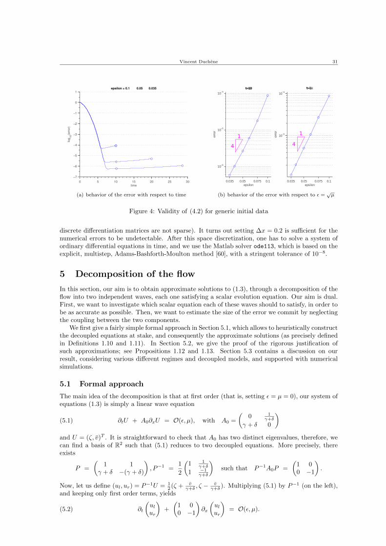
Vincent Duchene 31

0 5 10 15 20 25 30

−7

−6

−5

−4

−3

−2

−1

0

1epsilon = 0.1 0.05 0.035

time

log

10(e

rro

r)


0.035 0.05 0.075 0.1

10−6

10−5

10−4

t=10

epsilon

error

0.035 0.05 0.075 0.1

10−5

10−4

t=1/ε

epsilon

error

11

4 4


Figure 4: Validity of (4.2) for generic initial data

discrete differentiation matrices are not sparse). It turns out setting ∆x = 0.2 is sufficient for thenumerical errors to be undetectable. After this space discretization, one has to solve a system ofordinary differential equations in time, and we use the Matlab solver ode113, which is based on theexplicit, multistep, Adams-Bashforth-Moulton method [60], with a stringent tolerance of 10−8.

5 Decomposition of the flow

In this section, our aim is to obtain approximate solutions to (1.3), through a decomposition of theflow into two independent waves, each one satisfying a scalar evolution equation. Our aim is dual.First, we want to investigate which scalar equation each of these waves should to satisfy, in order tobe as accurate as possible. Then, we want to estimate the size of the error we commit by neglectingthe coupling between the two components.

We first give a fairly simple formal approach in Section 5.1, which allows to heuristically constructthe decoupled equations at stake, and consequently the approximate solutions (as precisely definedin Definitions 1.10 and 1.11). In Section 5.2, we give the proof of the rigorous justification ofsuch approximations; see Propositions 1.12 and 1.13. Section 5.3 contains a discussion on ourresult, considering various different regimes and decoupled models, and supported with numericalsimulations.

5.1 Formal approach

The main idea of the decomposition is that at first order (that is, setting ε = µ = 0), our system ofequations (1.3) is simply a linear wave equation

(5.1) ∂tU + A0∂xU = O(ε, µ), with A0 =

(0 1

γ+δ

γ + δ 0

)and U = (ζ, v)T . It is straightforward to check that A0 has two distinct eigenvalues, therefore, wecan find a basis of R2 such that (5.1) reduces to two decoupled equations. More precisely, thereexists

P =

(1 1

γ + δ −(γ + δ)

), P−1 =

1

2

(1 1

γ+δ

1 −1γ+δ

)such that P−1A0P =

(1 00 −1

).

Now, let us define (ul, ur) = P−1U = 12 (ζ + v

γ+δ , ζ −vγ+δ ). Multiplying (5.1) by P−1 (on the left),

and keeping only first order terms, yields

(5.2) ∂t

(ulur

)+

(1 00 −1

)∂x

(ulur

)= O(ε, µ).


As a conclusion, the solution U = (ζ, v)T may be decomposed in the following way:

U ≈(v+(x− t) + v−(x+ t) , (γ + δ)

(v+(x− t) + v−(x+ t)

))T.

Now, let us take into account the higher order terms in (1.3). One will make use of the followingstraightforward expansions:

h1h2

h1 + γh2=

1

γ + δ+ ε

δ2 − γ(γ + δ)2

ζ − ε2γδ(δ + 1)2

(γ + δ)3ζ2 − ε3

γδ2(δ + 1)2(1− γ)

(γ + δ)4ζ3 + O(ε4),

h12 − γh2

2

(h1 + γh2)2=

δ2 − γ(γ + δ)2

− 2εγδ(δ + 1)2

(γ + δ)3ζ − 3ε2

γδ2(δ + 1)2(1− γ)

(γ + δ)4ζ2 + O(ε3),

Q[h1, h2]v = − 1 + γδ

3δ(γ + δ)∂2xv − ε

γ + δ

3

((β − α)v∂2

xζ + (α+ 2β)∂x(ζ∂xv)− βζ∂2xv)

+ O(ε2),

R[h1, h2]v ≡ α

(1

2(∂xv)2 +

1

3v∂2xv

)+ O(ε)

with α =1− γ

(γ + δ)2and β =

(1 + γδ)(δ2 − γ)

δ(γ + δ)3.

Using the decomposition as above: (ul, ur) = P−1(ζ, v)T = 12 (ζ+ v

γ+δ , ζ−vγ+δ ), and withdrawing

every term of size O(µε2, ε4), one can check that the Green-Naghdi system (1.3) becomes thefollowing coupled system in terms of ul (left-going wave) and ur (right-going wave):

∂tul + ∂xul + f ε,µl (ul, ur) = 0,(5.3a)

∂tur − ∂xur + f ε,µr (ul, ur) = 0,(5.3b)

where f ε,µl and f ε,µl are defined below:

f ε,µl = εα1

2∂x((ul +

1

3ur)(ul − ur)

)+ ε2

α2

3∂x((ul − ur)ul(ul + ur)

)+ ε3

α3

4∂x((ul −

1

5ur)(ul − ur)(ul + ur)

2)

− µν∂2x∂t(ul − ur) + µεκ3∂x

(1

3(ul − ur)(∂2

xul − ∂2xur) +

1

2(∂xul − ∂xur)2

)− µε∂t

[κ1(ul∂

2xul − ur∂2

xur) + κ2(ur∂2xul − ul∂2

xur) + (κ1 +κ2

2)((∂xul)

2 − (∂xur)2)],

f ε,µr = −εα1

2∂x((1

3ul + ur)(ur − ul)

)− ε2α2

3∂x((ur − ul)ur(ul + ur)

)− ε3α3

4∂x((ur −

1

5ul)(ur − ul)(ul + ur)

2)

− µν∂2x∂t(ur − ul)− µεκ3∂x

(1

3(ur − ul)(∂2

xur − ∂2xul) +

1

2(∂xur − ∂xul)2

)− µε∂t

[κ1(ur∂

2xur − ul∂2

xul) + κ2(ul∂2xur − ur∂2

xul) + (κ1 +κ2

2)((∂xur)

2 − (∂xul)2)],

and where we used the notation

(5.4)α1 = 3

2δ2−γγ+δ , α2 = −3γδ(δ+1)2

(γ+δ)2 , α3 = −5 δ2(δ+1)2γ(1−γ)

(γ+δ)3 , ν = 16

1+γδδ(δ+γ) .

κ1 = (1+γδ)(δ2−γ)3δ(γ+δ)2 , κ2 = (1−γ)

3(γ+δ) , κ3 = γ−12(γ+δ) .

Remark 5.1. One could use higher order expansions with respect to the parameter ε, which wouldlead to decoupled models with formally higher accuracy. However, let us note that our results (seediscussion in Section 5.3) show that the main error of our decoupled models comes from neglectingcoupling terms which arise at low order, rather than the unidirectional error which is produced byneglecting higher order terms in the scalar equations. Thus including these higher order terms inthe evolution equation is unlikely to produce substantial improvement.

Vincent Duchene 33

Proposition 5.2 (Consistency of (5.3a)–(5.3b)). Let(upl , u

pr

)be strong solutions of (5.3a)–(5.3b),

depending on sets of parameters (ε, µ, δ, γ) = p ∈ P, as defined in (1.1). We assume that fors ≥ s0 > 1/2, upl , u

pr ∈ W 1([0, T );Hs+3(R)), uniformly in p. Additionally, we assume that there

exists h > 0 such that

hp1 ≡ 1− ε(upl + upr) ≥ h > 0, hp2 ≡1

δ+ ε(upl + upr) ≥ h > 0.

Then(ζp, vp

)T ≡ (upl + upr , (γ + δ)(upl − upr))

is consistent with Green-Naghdi equations (1.3) oforder s on [0, T ), at precision O(µε2 + ε4) (in the sense of Definition 1.2).

Proof. Proposition 5.2 is straightforward once one obtains a rigorous statement of the expansions

ofhp

1hp2

hp1+γhp

2

,(hp

1 )2−γ(hp2 )2

(hp1+γhp

2 )2 , Q[hp1, hp2]vp , R[hp1, h

p2]vp, as stated above, the residual being estimated

in W 1([0, T );Hs+1) norm. These expansions are easily checked, provided the assumptions of theproposition (upl , u

pr ∈ W 1([0, T );Hs+3(R)), hp1, h

p2 ≥ h > 0) are satisfied, and using uniformly

continuous (for s ≥ s0 > 1/2) Sobolev embedding Hs → L∞.

The decoupled approximation simply consists in neglecting all coupling terms in (5.3a)–(5.3b),that is replacing f ε,µl (ul, ur) by f ε,µl (ul, 0), and f ε,µr (ul, ur) by f ε,µr (0, ur). This yields

∂tul + ∂xul + εα1ul∂xul + ε2α2u2l ∂xul + ε3α3ul

3∂xul − µν∂2x∂tul

−µε∂t(κ1ul∂

2xul + (κ1 + 1/2κ2)(∂xul)

2)

+ µεκ3∂x(1

3ul∂

2xul +

1

2(∂xul)

2)

= 0,(5.5a)

∂tur − ∂xur − εα1ur∂xur − ε2α2u2r∂xur − ε3α3ur

3∂xur − µν∂2x∂tur

−µε∂t(κ1ur∂

2xur + (κ1 + 1/2κ2)(∂xur)

2)− µεκ3∂x

(1

3ur∂

2xur +

1

2(∂xur)

2)

= 0,(5.5b)

and (5.5a)–(5.5b) are the decoupled equations we consider; see Definition 1.10.

Let us now reckon that one can deduce from (5.5a)–(5.5b) a large family of formally equivalentmodels, with different parameters, following the techniques used for example in [7, 8, 20, 25], andthat we discuss below.

• The BBM trick (from Benjamin-Bona-Mahony [6]). Keeping only the first order terms inequations (5.5a)–(5.5b), one has the simple transport equations

∂tul + ∂xul = O(µ, ε), and ∂tur − ∂xur = O(µ, ε).

It follows that one can replace time derivatives in higher order terms (of orderO(µε)) by spatialderivatives (up to a sign), and both equations have formally the same order of accuracy. Inorder to simplify, we consider only equations with spatial derivatives in O(µε) terms (if theyexist). In particular, (5.5a)–(5.5b) becomes


3∂xul − µν∂2x∂tul

+µε∂x((κ1 + 1/3κ3)ul∂

2xul + (κ1 + 1/2κ2 + 1/2κ3)(∂xul)

2)

= 0,(5.6a)


3∂xur − µν∂2x∂tur

−µε∂x((κ1 + 1/3κ3)ur∂

2xur + (κ1 + 1/2κ2 + 1/2κ3)(∂xur)

2)

= 0.(5.6b)

Following a similar idea, we make use of the low order identity obtained from (5.6a)–(5.6b):

∂tul + ∂xul + εα1ul∂xul = O(µ, ε2),

so that one has, for any θ ∈ R,

∂tul = θ∂tul + (θ − 1)(∂xul + εα1ul∂xul

)+ O(µ, ε2).


Plugging back into (5.6a) and withdrawing O(µ2, µε2) terms yields


3∂xul − µνθt ∂2x∂tul

+ µνθx∂3xul + µε∂x

(κθ1ul∂

2xul + κθ2(∂xul)

2)

= 0,(5.7a)


3∂xur − µνθt ∂2x∂tur

− µθxν∂3xur − µε∂x

(κθ1ur∂

2xur + κθ2(∂xur)

2)

= 0,(5.7b)

where we have defined, after parameters (5.4),

(5.8) νθt ≡ θν, νθx ≡ (1−θ)ν, κθ1 ≡ κ1 +κ3

3+(1−θ)α1ν, κθ2 ≡ κ1 +

κ2

2+κ3

2+(1−θ)α1ν.

• Near identity changes of variables. We used system (1.3) as our reference system, and thereforethe unknowns we consider are (ζ, v), where v = u2 − γu1 is the shear layer-mean velocity.However, other natural variables may also be used, such as the the shear velocity at theinterface (leading to system (2.17))

v0 = ∂x((φ2 − γφ1

)|z=εζ

)= ∂x

(φ2(x, r2(x, 0))− γφ1(x, r1(x, 0))

),

(where we use the change of coordinate flattening the fluid domains: ri(x, z) = zhi(x)+εζ(x);see [24]), or more generally, using the horizontal derivative of the potential at specific heights(z1, z2) ∈ [0, 1)× (−1, 0]:

vz1,z2 = ∂x

(φ2(x, r2(x, z2))− γφ1(x, r2(x, z1))

).

Using the expansion of the velocity potentials and layer-mean velocities, as obtained in [24],as well as the identity h1u1 + h2u2 = 0 (obtained through the rigid lid assumption), yieldsthe following approximation:

vz1,z2 = v + µλz1,z2∂2xv + µεT z1,z2(ζ, v) + O(µ2, µε2),

with λz1,z2 = − (3z22 + 6z2 + 2) + γδ(3z2

1 − 6z1 + 2)

6δ(γ + δ), and T z1,z2 a bi-linear differential oper-

ator whose precise formula do not play a significant role in our work as we shall discuss below.Following this idea, we consider

uλl ≡ ul + µλ∂2xul ,

uλr ≡ ur − µλ∂2xur .

If (ul, ur) satisfies (5.7a)–(5.7b), then (uλl , uλr ) satisfies the following equations, up to terms

of order O(µ2, µε2):

∂tuλl + ∂xu

λl + εα1u

λl ∂xu

λl + ε2α2u

λl

2∂xu

λl + ε3α3u

λl

3∂xu

λl − µνθ,λt ∂2

x∂tuλl

+ µνθ,λx ∂3xu

λl + µε∂x

(κθ,λ1 uλl ∂

2xu

λl + κθ2(∂xu

λl )2)

= 0,(5.9a)

∂tuλr − ∂xu

λr − εα1u

λr∂xu

λr − ε2α2u

λr

2∂xu

λr − ε3α3u

λr

3∂xu

λr − µνθ,λt ∂2

x∂tuλr

− µνθ.λx ∂3xu

λr − µε∂x

(κθ,λ1 uλr∂

2xu

λr + κθ2(∂xu

λr )2)

= 0,(5.9b)

where we have defined, after parameters (5.8),

(5.10) νθ,λt ≡ νθt + λ, νθ,λx ≡ νθx − λ, κθ,λ1 ≡ κθ,λ1 + α1λ.

Note that in order to fit as much as possible with variables (ζ, vz1,z2), one could have usedmore complex change of variables, such as

uλl ≡ ul + µλ∂2xul + µε

(λ2ul∂

2xul + λ3∂x(ul

2)),

uλr ≡ ur − µλ∂2xur − µε

(λ2ur∂

2xur + λ3∂x(ur

2)),

Vincent Duchene 35

with λ = λz1,z2

2(γ+δ) , and λ2, λ3 obtained through T z1,z2 . It turns out uλl and uλr would then

satisfy the same equation as above: the new parameters do not depend on λ2 and λ3, as theircontribution is of order O(µε2, µ2ε), after using BBM trick to suppress higher order derivativeswith respect to time. We thus do not consider such changes of variable.

Ultimately, one obtains the family of approximations described in Definition 1.10, with thefollowing set of parameters:

(5.11)

α1 =3

2

δ2 − γγ + δ

, α2 = −3γδ(δ + 1)2

(γ + δ)2, α3 = −5

δ2(δ + 1)2γ(1− γ)

(γ + δ)3,

νθ,λt ≡ θ

6

1 + γδ

δ(δ + γ)+ λ, νθ,λx ≡ 1− θ

6

1 + γδ

δ(δ + γ)− λ,

κθ,λ1 ≡ (1 + γδ)(δ2 − γ)

3δ(γ + δ)2(1 +

1− θ4

)− (1− γ)

6(γ + δ)+ λ

3

2

δ2 − γγ + δ

,

κθ2 ≡(1 + γδ)(δ2 − γ)

3δ(γ + δ)2(1 +

1− θ4

)− (1− γ)

12(γ + δ).

5.2 Rigorous justification; proof of Proposition 1.12

In this section, we give the rigorous justification of the Constantin-Lannes decoupled approximation,as defined in Definition 1.10. More precisely, we prove Proposition 1.12, that we recall below.

Proposition 5.3 (Consistency). Let ζ0, v0 ∈ Hs+6, with s ≥ s0 > 3/2. For (ε, µ, δ, γ) = p ∈ P,as defined in (1.1), we denote Up

CL the unique solution of the CL approximation, as defined inDefinition 1.10. For some given M?

s+6 > 0, sufficiently big, we assume that there exists T ? > 0 anda family (Up

CL)p∈P such that

T ? = max(T ≥ 0 such that

∥∥UpCL

∥∥L∞([0,T );Hs+6)

+∥∥∂tUp

CL

∥∥L∞([0,T );Hs+5)

≤ M?s+6

).

Then there exists U c = U c[UpCL] such that U ≡ Up

CL + U c is consistent with Green-Naghdiequations (1.3) of order s on [0, t] for t < T ?, at precision O(ε?CL) with

ε?CL = C max(ε2(δ2 − γ)2, ε4, µ2) (1 +√t),

with C = C( 1s0−3/2 ,M

?s+6,

1δmin

, δmax, εmax, µmax, |λ|, |θ|), and the corrector term U c is estimated as∥∥U c∥∥L∞([0,T?];Hs)

+∥∥∂tU c∥∥L∞([0,T?];Hs)

≤ C max(ε(δ2 − γ), ε2, µ) min(t,√t).

Additionally, if there exists α > 1/2, M ]s+6, T

] > 0 such that

6∑k=0

∥∥(1 + x2)α∂kxUpCL

∥∥L∞([0,T );Hs)

+

5∑k=0

∥∥(1 + x2)α∂kx∂tUpCL

∥∥L∞([0,T );Hs)

≤ M ]s+6 ,

then U ≡ UpCL + U c is consistent with Green-Naghdi equations (1.3) of order s on [0, t] for t < T ],

at precision O(ε]CL) with

ε]CL = C max(ε2(δ2 − γ)2, ε4, µ2),

with C = C( 1s0−3/2 ,M

]s+6,

1δmin

, δmax, εmax, µmax, |λ|, |θ|) and U c is uniformly estimated as∥∥U c∥∥L∞([0,T ]];Hs)

+∥∥∂tU c∥∥L∞([0,T ]];Hs)

≤ C max(ε(δ2 − γ), ε2, µ) min(t, 1).

Remark 5.4. The proof of Proposition 1.13 is identical to the one of Proposition 5.3, presentedbelow. More precisely, the choice of lower-order evolution equations modifies mostly the last termof (5.16) in Lemma 5.7 (below), as the contribution of neglected unidirectional terms should beadded. The additional error is therefore uniformly bounded over times [0, T ?] and [0, T ]]. Thedetailed proof of Proposition 1.13 is omitted.


Strategy of the proof. Our strategy is the following. Inspired by the calculations of Section 5.1,we seek an approximate solution of (1.3) under the form

Uapp ≡(v+(t, x− t) + v−(t, x+ t), (γ + δ)

(v+(t, x− t)− v−(t, x+ t)

))+ σUc[v±] ,

where v± satisfies the Constantin-Lannes equation (1.5), and Uc contains the leading order couplingterms. The parameter σ is assumed to be small, and we want to justify our approximate solutionsover times of order O(1/σ).

Precisely, our aim is to prove that

i. the coupling term σUc can be controlled, and grows sublinearly in time;

ii. the approximate function Uapp solves the coupled equation (1.3), up to a small remainder.

As we shall see, controlling the secular growth of Uc requires to consider separately the short timescale, where the coupling effects may be strong, and long time scale, where the coupling betweentwo localized waves moving in opposite directions can be controlled. Thus we introduce the longtime scale τ = t/σ, and will seek an approximate solution of (1.3) as

Uapp(t, x) = Uapp(σt, t, x), with

Uapp(τ, t, x) =(v+(τ, t, x) + v−(τ, t, x) , (γ + δ)

(v+(τ, t, x)− v−(τ, t, x)

))+ σUc[v±](τ, t, x) ,

with obvious misuses of notation.Plugging the Ansatz into the coupled Green-Naghdi equation (1.3) yields at first order

(5.12) ∂tv+ + ∂xv+ = 0 and ∂tv− − ∂xv− = 0,

so that v±(τ, t, x) = v±(τ, x±) ≡ v±(τ, x∓ t).At next order, and following the calculations of Section 5.1, one obtains the decoupled equations

σ(1− µνt∂2x)∂τ v± ± εα1v±∂xv± ± ε2α2(v±)2∂xv± ± ε3α3(v±)3∂xv±(5.13)

± µ(νx + νt)∂3xv± ± µε∂x

(κ1v±∂

2xv± + κ2(∂xv±)2

)= 0,

where parameters satisfy identities of Definition 1.10. In order to deal with the coupling terms, weintroduce the following first order correction.

Definition 5.5. We denote U c ≡ (uc+ +uc−, (γ+δ)(uc+−uc−))

where uc±[v±](τ, t, x) satisfies initialcondition uc± |t=0 ≡ 0, and equation(5.14)σ(∂t + ∂x)uc+ + f l(v+, v−)− f l(v+, 0) = 0, and σ(∂t − ∂x)uc− + fr(v+, v−)− fr(0, v−) = 0,

where f l and fr are defined as in (5.3a)–(5.3b).

Remark 5.6. The above discussion does not take into account the use of near identity change ofvariable as described in Section 5.1. In that case, we set the initial data as follows:

(5.15) v± |τ=0 = (1± µλ∂2x)

(ζ0 ± v0

γ+δ

2

).

Thus the function v±(σt, x∓ t) , defined by (5.13) and with initial data (5.15), satisfies precisely

v±(σt, t, x) = v±(σt, x∓ t) = vλ±(t, x∓ t),

where vλ± is the solution of (1.5) as defined in Definition 1.10.

The proof is now as follows. First, we state that the approximate solution, Uapp(σt, t, x), con-structed as above, does satisfy (1.3), up to a small remainder (although depending on the size of v±,uc±, and their derivatives). The fact that v± is uniformly bounded follows from the assumptions ofthe proposition. The key ingredient in the proof consists in estimating the growth over long times(that is, in the variable τ), of uc± satisfying (5.14). Each of these steps are described in details inthe following.

Vincent Duchene 37

Construction and accuracy of the approximate solution Uapp. The following Lemma statescarefully the definition of our approximate solution Uapp, and its precision in the sense of consistency.

Lemma 5.7. Let ζ0, v0 ∈ Hs+6, with s ≥ s0 > 3/2, and (ε, µ, δ, γ) = p ∈ P, as defined in (1.1).Let vλ±(τ, t, x) be defined by (5.12), (5.13) and with initial data (5.15). Then define v±(τ, t, x) as

v±(τ, t, x) = (1± µλ∂2x)−1vλ±(τ, t, x) ,

and set

Uapp(τ, t, x) =(v+(τ, t, x) + v−(τ, t, x) , (γ + δ)

(v+(τ, t, x)− v−(τ, t, x)

))+ σUc[v±](τ, t, x),

where U c is defined in Definition 5.5. Then for ε small enough, Uapp(σt, t, x) satisfies the coupledequations (1.3), up to a remainder, R, bounded by∣∣R∣∣

Hs≤ F

(ε4(∣∣v±∣∣Hs+1 + σ

∣∣uc±∣∣Hs+1) + µε2(∣∣v±∣∣Hs+3 +

∣∣∂tv±∣∣Hs+2 + σ∣∣uc±∣∣Hs+3 + σ

∣∣uc±∣∣Hs+2)

+σ2∣∣∂τuc± ∣∣Hs + εα1σ

∣∣uc± ∣∣Hs+1

(∣∣v± ∣∣Hs+1 + σ∣∣uc± ∣∣Hs+1

)+ ε2σ(

∣∣uc± ∣∣Hs+1

∣∣v± ∣∣Hs+1)

+ µσ(∣∣∂3

xuc±∣∣Hs

+∣∣∂2x∂tu

c±∣∣Hs

) (1 + ε

(∣∣∂3xv±

∣∣Hs

+∣∣∂2x∂tv±

∣∣Hs

))+ max(ε4, µε2, µ2)C(

∣∣v±∣∣Hs+5 +∣∣∂tv±∣∣Hs+4)

),(5.16)

with a function F satisfying F (X) ≤ C( 1s0−3/2 ,M

?s+6,

1δmin

, δmax, εmax, µmax, |λ|, |θ|)X.

Proof. This result a direct application of the definitions above, and calculations presented in Sec-tion 5.1. More precisely, one obtains

R = R0 + σ2∂τuc± +

(f(v+ + σuc+, v− + σuc−)− f(v+, v−)

)+ Rθ +Rλ,

where

• R0 is the contribution due to the expansion of h1h2

h1+γh2, h1

2−γh22

(h1+γh2)2 ,Q[h1, h2]v and R[h1, h2]v

with respect to parameter ε;

• f is a linear combination of f ε,µl and f ε,µr as defined in (5.3a)–(5.3b);

• Rθ and Rλ are respectively the components due to the use of the BBM trick and near-identitychange of variable.

Let us detail the first terms leading to R0. We want to control the contribution of the expansionof h1h2

h1+γh2, that is, more precisely, estimate

∣∣∣R(1)0

∣∣∣Hs+1

=

∣∣∣∣ h1h2

h1 + γh2− 1

γ + δ− ε δ

2 − γ(γ + δ)2

ζ + ε2γδ(δ + 1)2

(γ + δ)3ζ2 + ε3

γδ2(δ + 1)2(1− γ)

(γ + δ)4ζ3

∣∣∣∣Hs+1

,

where we denote ζ = ζapp = (v+ + v− + σ(uc+ + uc))(σt, t, x), and h1 = 1− εζapp, h2 = 1δ + εζapp.

Note that, as we shall prove that ζapp is bounded in L∞([0, T ?);Hs+1), there exists ε0 > 0 suchthat for any 0 ≤ ε < ε0, one has∣∣ζ∣∣

L∞< min(1, 1/δ) and

∣∣ 1

h1 + γh2

∣∣Hs+1 ≤

1

2(1 + γ/δ).

Now, one can easily check that, in that case, R(1)0 = ε4 P

(1)(ζ)h1+γh2

, where P (1)(X) is a polynomial of

degree 4, and estimate∣∣∣R(1)

0

∣∣∣Hs+1

≤ ε4F (∣∣v± ∣∣Hs+1 + σ

∣∣uc± ∣∣Hs+1) follows.

As h1h2

h1+γh2gets multiplied by v and differentiated once, the first term in (5.16) follows.

The contributions due to the expansion of h12−γh2

2

(h1+γh2)2 is estimated in the same way. The contri-

bution due to the expansion of R[h1, h2]v requires more derivatives, but may be estimated as above


by µε2F(∣∣v±∣∣Hs+3 + σ

∣∣uc±∣∣Hs+3

). The contribution due to the expansion of Q[h1, h2]v involves

one time derivative, and is controlled by µε2F(∣∣∂tv±∣∣Hs+2 + σ

∣∣uc±∣∣Hs+2

). This yields the first line

of (5.16).

Then, one can check that

f ε,µl (v+ + σuc+, v− + σuc−)− f ε,µl (v+, v−) = ∂x(P (σuc±, v±)

)+ µσν∂2

x∂tuc±

+ µε∂x

(Q1(σuc±, ∂

2xv±) +Q2(σ∂xu

c±, ∂xv±) +Q3(σ∂2

xuc±, v±) +Q4(σuc±, ∂

2xu

c±) +Q5(σ∂xu

c±, ∂xv±)

)+ µε∂t

(Q6(σuc±, ∂

2xv±) +Q7(σ∂xu

c±, ∂xv±) +Q8(σ∂2

xuc±, v±) +Q9(σuc±, ∂

2xu

c±) +Q10(σ∂xu

c±, ∂xv±)

),

where P is a bivariate polynomial of degree 4, and whose leading order terms are

P (σuc±, v±) = α1ε(σuc±v±) + ε(σuc±)2 + α2ε

2σuc±v±2 + . . . ,

and Qi are bilinear forms. Each of these terms are bounded as in (5.16).Finally, Rθ and Rλ depend uniquely on decoupled terms v±, and one has similarly∣∣Rθ∣∣Hs +

∣∣Rλ∣∣Hs ≤ C0 max(ε4, µε2, µ2)(∣∣v±∣∣Hs+5 +

∣∣∂tv±∣∣Hs+4),

with C0 = C( 1s0−3/2 ,

1δmin

, δmax, εmax, µmax, |λ|, |θ|). The proposition follows.

Our aim is now to estimate each of the terms in (5.16).

Estimates of the decoupled approximation v±. The bound on v± is a direct consequence ofthe assumptions of the Proposition, using the identity

v±(σt, t, x) = v±(σt, x∓ t) = v±(t, x∓ t),

where v±(t, x∓t) is defined through Definition 1.10, and therefore is uniformly controlled as assumedin the Proposition. It follows

(5.17)∥∥v±∥∥L∞([0,σT?)×[0,T?);Hs+6)

+ σ∥∥∂τ v±∥∥L∞([0,σT?)×[0,T?);Hs+5)

≤ M?s+6.

However, let us note that one can gain extra smallness on σ∂τ v± (trading with a loss of deriva-tives) from the fact that v± satisfies (5.13). Indeed, one has for any k ∈ N,

σ∣∣∂τ v±∣∣Hs+k ≤ max(εα1, ε

2, µ)P (∣∣v±∣∣Hs+k+3) + µνtσ

∣∣∂2x∂τ v±

∣∣Hs+k

,

where P (X) is a polynomial, so that 8

(5.18) σ∥∥∂τ v±∥∥L∞([0,σT?)×[0,T?);Hs+3)

≤ max(εα1, ε2, µ)C(M?

s+6).

As for the case of localized initial data, the assumption of the Proposition yields

(5.19)

6∑k=0

∥∥(1+x2)α∂kxv±∥∥L∞([0,σT ])×[0,T ]);Hs

+

5∑k=0

σ∥∥(1+x2)α∂τv±

∥∥L∞([0,σT ])×[0,T ]);Hs

≤M ]s+6.

and one deduces as above, for k = 0, 1, 2, 3

σ∣∣(1 + x2)α∂kx∂τ v±

∣∣Hs≤ max(εα1, ε

2, µ)P

(3∑i=0

∣∣(1 + x2)α∂k+ix v±

∣∣Hs

)+ µσ

∣∣(1 + x2)α∂k+2x ∂τ v±

∣∣Hs

≤ max(εα1, ε2, µ)C(M ]

s+6).(5.20)

8Here and in the following, we do not explicitly keep track of the dependence with respect to all the parameters;as (ε, µ, δ, γ) = p ∈ P, as defined in (1.1), and parameters satisfy identities of Definition 1.10, one should replaceC(M?

s+6) by C( 1s0−3/2

,M?s+6,

1δmin

, δmax, εmax, µmax, |λ|, |θ|).

Vincent Duchene 39

Control of the secular growth of the coupling terms uc±. Let us now study the termU c ≡ (uc+ + uc−, (γ + δ)(uc+ − uc−)

), which contains all the coupling effects between the different

components. Our aim is to control the secular growth of this term. This will be achieved throughthe following two Lemmas.

Lemma 5.8. Let s ≥ 0, and f0 ∈ Hs+1(R). Then there exists a unique global strong solution,u(t, x) ∈ C0(R;Hs+1) ∩ C1(R;Hs), of

(∂t + c1∂x)u = ∂xfu |t=0 = 0

with

(∂t + c2∂x)f = 0fi |t=0 = f0

where c1 6= c2.Moreover, one has the following estimates for any t ∈ R:∣∣u(t, ·)

∣∣Hs+1(R)

≤ 2

|c1 − c2|∣∣f0∣∣Hs+1(R)

,∣∣u(t, ·)

∣∣Hs(R)

≤ |t|∣∣f0∣∣Hs+1(R)

.

Lemma 5.9. Let s ≥ s0 > 1/2, and v01, v0

2 ∈ Hs+1(R). Then there exists a unique global strongsolution, u ∈ C0(R;Hs+1) ∩ C1(R;Hs), of

(∂t + c∂x)u = g(v1, v2)u |t=0 = 0

with ∀i ∈ 1, 2,

(∂t + ci∂x)vi = 0vi |t=0 = v0

i

where c1 6= c2, and g is a bilinear mapping defined on R2 and with values in R.Moreover, one has the following estimates:

i. ∥∥u∥∥L∞([0,t);Hs)

≤ Cs0 t|∣∣v0

1

∣∣Hs(R)

∣∣v02

∣∣Hs(R)

,∥∥∂tu∥∥L∞([0,t);Hs)

≤ Cs0 |t|∣∣v0

1

∣∣Hs+1(R)

∣∣v02

∣∣Hs+1(R)

.

ii. Using c1 6= c2, one has the sublinear growth

∣∣u(t, ·)∣∣Hs(R)

= Cs0

√t√

|c1 − c2|∣∣v0

1

∣∣Hs

∣∣v02

∣∣Hs

∣∣∂tu(t, ·)∣∣Hs

= Cs01 +√t√

|c1 − c2|∣∣v0

1

∣∣Hs+1

∣∣v02

∣∣Hs+1 ,

with Cs0 = C( 1s0−1/2 ).

iii. If moreover, there exists α > 1/2 such that v01(1 + x2)α, and v0

2(1 + x2)α ∈ Hs(R), then onehas the (uniform in time) estimate∥∥u∥∥

L∞Hs(R)≤ Cs0

∣∣v01(1 + x2)α

∣∣Hs(R)

∣∣v02(1 + x2)α

∣∣Hs(R)

,

with Cs0 = C( 1s0−1/2 ,

1c1−c2 ,

1α−1/2 ).

Proof. Lemma 5.8 is straightforward, since one has an explicit expression for the solution:

u(t, x) =1

c2 − c1(f(t, x+ (c2 − c1)t)− f(t, x)

)=

1

c2 − c1(f0(x− c1t)− f0(x− c2t)

).

It follows∣∣u∣∣

Hs+1 ≤ 2|c2−c1|

∣∣f0∣∣Hs+1 , and

∣∣u∣∣Hs

=1

|c2 − c1|∣∣ ∫ c1t

c2t

∂xf0(x− y) dy

∣∣Hsx≤ 1

|c2 − c1|

∫ c1t

c2t

∣∣∂xf0(x− y)∣∣Hsx

dy ≤ |t|∣∣∂xf0

∣∣Hs.

As for Lemma 5.9, the well-posedness as well as estimate i. are standard; the remaining esti-mates, controlling the secular growth, are proved in [45], Propositions 3.2 and 3.5.

One can now state our key result, concerning the control of the secular growth of U c.


Lemma 5.10. Let v± defined as in Lemma 5.7, for (τ, t, x) ∈ [0, σT ?) × [0, T ?) × R. Then thereexists a unique Uc(τ, t, x) ∈ L∞([0, T )×R;Hs) such that U c ≡ (uc+ + uc−, (γ + δ)(uc+ − uc−)

), with

uc± satisfying (5.14) and U c |t=0 ≡ 0. Moreover, one has the estimate for and t ∈ [0, T ?]

σ∥∥uc±∥∥L∞([0,σT?]×[0,t];Hs)

≤ C(M?s+3) max(εα1, ε

2, µ) min(t,√t),(5.21)

σ2∥∥∂τuc±∥∥L∞([0,T ]×[0,t];Hs)

≤ C(M?s+6) max(εα1, ε

2, µ)2 min(t,√t).(5.22)

Moreover, if (1 + x2)ζ0, (1 + x2)v0 ∈ Hs+3, s ≥ s0 > 1/2, and ζ0, v0 ∈ Hs+3+2m, then one hasthe uniform estimate

σ∥∥uc±∥∥L∞([0,σT ]]×[0,T ]];Hs)

≤ C(M ]s+3) max(εα1, ε

2, µ) min(t, 1),(5.23)

σ2∥∥∂τuc±∥∥L∞([0,T ]×[0,T ]];Hs)

≤ C(M ]s+6) max(εα1, ε

2, µ)2 min(t, 1).(5.24)

Proof. The function uc± are defined as the solutions of a transport equation, with a known andcontrolled forcing term, thus the existence and uniqueness of uc± and U c is straightforward.

As for the estimates, we focus below on uc+. Estimates for uc− follow in the same way.By definition, uc+ satisfies

σ(∂t + ∂x)uc+ = f l(v+, 0) − f l(v+, v−),

and the right-hand-side can be decomposed in the following way:

f l(v+, 0) − f l(v+, v−) =

3∑j=1

ajεj∂x(vj+1−)

+

3∑j=1

εjj∑i=1

ai,j∂x(vi+v

j−i+1− ) + µb∂3

xv−

+ µε∂x(c1v−∂2xv− + c2(∂xv−)2) + µε

3∑k=0

dk(∂kxv+)(∂3−kx v−)

≡3∑j=1

εj∂xfj +

3∑j=1

εjj∑i=1

gi,j + µ∂xf4 + µε∂xf5 + µε

3∑k=0

gk,

where the parameters aj , ai,j , bj , cj and dk depend on γ, δ, λ, θ, and where we used ∂tv− = ∂xv−.

Note that the first order terms εa1 and εa1,1 are factored by α1 = 32δ2−γγ+δ .

The contribution from fj , j = 1, . . . , 5 are estimated thanks to Lemma 5.8, whereas we useLemma 5.9 for the contribution of gi,j and gk.

For all 0 ≤ j ≤ 4, one has ∂tfj − ∂xfj = 0, and

•∣∣fj∣∣Hs+1 ≤ C

∣∣v−∣∣L∞ ∣∣v−∣∣Hs+1 ≤ C(∣∣v−(τ, ·)

∣∣Hs+1), for j = 1, 2, 3;

•∣∣f4

∣∣Hs+1 ≤ C

∣∣∂2xv−

∣∣Hs+1 ≤ C(

∣∣v−(τ, ·)∣∣Hs+3);

•∣∣f5

∣∣Hs+1 ≤ C

∣∣v−∣∣L∞ ∣∣∂2xv−

∣∣Hs+1 +

∣∣(∂xv−)2∣∣Hs+1 ≤ C(

∣∣v−(τ, ·)∣∣Hs+3).

It is then straightforward to check that gij and gk are the sum of bilinear mappings, applied tofunctions v±, satisfying ∂tv± ± ∂xv± = 0, with v± bounded as below:

•∣∣vi±∣∣Hs ≤ C(

∣∣v±∣∣Hs) ≤ C(∣∣v±(τ, ·)

∣∣Hs

), for i = 1, 2, 3.

•∣∣∂xvj±∣∣Hs ≤ C(

∣∣v±∣∣Hs+1) ≤ C(∣∣v±(τ, ·)

∣∣Hs+1), for j = 1, 2, 3.

•∣∣∂kxv±∣∣Hs ≤ µC(

∣∣v±∣∣Hs+k) ≤ C(∣∣v±(τ, ·)

∣∣Hs+3), for k = 0, 1, 2, 3.

It follows form Lemmata 5.8 and 5.9 that uc+ satisfies

σ∣∣uc+(τ, t, ·)

∣∣Hs≤ min(t,

√t) max(α1ε, ε

2, µ, µε)C(∣∣v±(τ, ·)

∣∣Hs+3

),

and the last term is uniformly estimated through (5.17), so that (5.21) follows.

Vincent Duchene 41

As for the case of localized initial data, we make use of the fact that for k = 0, 1, 2, 3, one has∣∣(1 + x2)α∂kx v±(τ, t, ·)∣∣Hs

=∣∣(1 + x2)α∂kx v±(τ, 0, ·)

∣∣Hs

=∣∣(1 + x2)α∂kxv

λ±(τ/σ, ·)

∣∣Hs≤ M ]

s+3,

so that (5.23) follows in the same way for τ ≤ σT ].

The estimates on ∂τv±(τ, x) are obtained similarly, as

(∂t + ∂x)∂τuc+ ≡

3∑j=1

εj∂x∂τfj +

3∑j=1

εjj∑i=1

∂τgi,j + µ∂x∂τf4 + µε∂x∂τf5 + µε

3∑k=0

∂τgk.

One can check that each term of the right hand side satisfies the hypotheses of Lemmata 5.8 or 5.9,and estimate (5.18) allows to obtain (5.22).

The case of weighted Sobolev spaces (5.24) follows as above, using estimate (5.20). The Lemmais proved.

Completion of the proof. The consistency result stated in Proposition 5.3 is now a straight-forward consequence of Lemma 5.7, together with estimates (5.17)–(5.19), and Lemma 5.10.

One can check that the remainder in Lemma 5.7 can be estimated as∣∣R∣∣Hs≤ C(M?

s+6)(

max(α21ε

2, ε4, µ2) min(t,√t) + max(ε4, µ2)

)Note that we use

∂t(v±(σt, t, x)

)= σ∂τ v± + ∂tv±, and σ

∣∣∂τ v±∣∣Hs ≤ max(εα1, ε2, µε)

∣∣v±∣∣Hs+2 ,

as above, as well as a uniform estimate

σ∥∥ uc± ∥∥L∞([0,T?;Hs+1)

≤ M.

The latter estimate can be enforced using Lemma 5.10, by restricting the time interval with

(T ?)1/2 ≤ M

max(εα1, ε2, µ),

although such condition is not necessary, as Proposition 5.3 is empty for t ≥M(max(εα1, ε2, µ))−2,

the accuracy of the decoupled solutions being of order O(1).

More precisely, we proved the following Lemma.

Lemma 5.11. For ζ0, v0 ∈ Hs+6, with s ≥ s0 > 3/2, and (ε, µ, δ, γ) = p ∈ A, as defined in 1.1, letUapp be defined as in Lemma 5.7. Then Uapp(σt, t, x) satisfies the coupled equations (1.3), up to aremainder, R, estimated for t ∈ [0, T ?) by

∥∥R∥∥L∞([0,t);Hs)

≤ C(M?s+6)

(max(α2

1ε2, ε4, µ2) min(t,

√t) + max(ε4, µ2)

),

and on [0, T ]) by

∥∥R∥∥L∞([0,t);Hs)

≤ C(M ]s+6)

(max(α2

1ε2, ε4, µ2) min(t, 1) + max(ε4, µ2)

).

Proposition 5.3 is a consequence of the above Lemma, together with the estimates of Lemma 5.10(see also Remark 5.6).


5.3 Discussion

Our result takes its full meaning in the light of a conjectured stability result on Green-Naghdiequations (1.3), or any consistent model, as described in Hypothesis 1.3. If such a result holds,then one can deduce from the consistency result of Proposition 1.12 that the difference betweenthe solution of the Green-Naghdi system (1.3) (and in the same way, the solution of the full Eulersystem if it exists) and the weakly coupled approximate solution U ≡ UCL + U c is small. Theestimates concerning the difference between the solution of (1.3) and the fully decoupled solutionUCL simply follows from the estimates on Uc, in Proposition 1.12. This strategy has been used inthe water-wave case in [8], and in the case of internal waves (when restricting to the long waveregime) in [25].

Throughout this section, we assume that Hypothesis 1.3 holds, and study the convergenceresults between solutions of the Green-Naghdi model and the different approximate solutions whichproceeds.

Let us first state the convergence results concerning the weakly coupled model, defined in Propo-sition 1.12.

Corollary 5.12 (Convergence of weakly coupled model). For (ε, µ, δ, γ) = p ∈ P, as definedin (1.1), let Up

GN be a solution of Green-Naghdi equations (1.3) such that the family (UpGN) is

uniformly bounded on Hs, s sufficiently big, over time interval [0, TGN]. Assume that hypothesesof Proposition 1.12 hold, and denote Up ≡ Up

CL + U c[UpCL] the approximate solution, satisfying

UGNp |t=0 = Up |t=0 . Then if Hypothesis 1.3 is valid, for any t ≤ min(TGN, T

?s+6), one has∥∥Up − Up

GN

∥∥L∞([0,t];Hs)

≤ C max(ε2(δ2 − γ)2, ε4, µ2) t(1 +√t),

with C = C(∥∥Up

GN

∥∥L∞([0,TGN];Hs)

,M?s+6,

1δmin


If moreover, the initial data is sufficiently localized in space, then one has for t ≤ min(TGN, T]s+6),∥∥Up − Up

GN

∥∥L∞([0,t];Hs)

≤ C max(ε2(δ2 − γ)2, ε4, µ2) t,

with C = C(∥∥Up

GN

∥∥L∞([0,T ];Hs)

,M ]s+6,

1δmin


We therefore see that the weakly coupled model achieves the same accuracy as the fully coupledGreen-Naghdi model, in the Camassa-Holm regime (1.2), if one restricts to critical case δ2 − γ =O(µ), and if the initial data is sufficiently localized in space.

Let us now turn to the fully decoupled models. The following result is a straightforward appli-cation of the above Corollary, together with the estimate of Proposition 1.12. Estimates concerninglower order decoupled models are obtained in the same way, using Proposition 1.13.

Corollary 5.13 (Convergence of decoupled models). For (ε, µ, δ, γ) = p ∈ P, as defined in (1.1), letUpGN be a solution of Green-Naghdi equations (1.3) such that the family (Up

GN) is uniformly boundedon Hs, s sufficiently big, over time interval [0, TGN]. Denote respectively Up

CL, UpeKdV, U

pKdV, U

piB

the decoupled approximations defined in Definitions 1.10 and 1.11. Assume that the hypotheses ofProposition 1.12 hold, and Hypothesis 1.3 is valid. Define ε0 = max(ε(δ2− γ), ε2, µ). Then for anyt ≤ min(TGN, T

?s+6), one has∥∥Up

CL − UGNp∥∥L∞([0,t];Hs)

≤ C ε0 min(t, t1/2)(1 + ε0t),∥∥UpeKdV − UGN

p∥∥L∞([0,t];Hs)

≤ C ε0 min(t, t1/2)(1 + ε0t) + C max(ε3, µε) t,∥∥UpKdV − UGN

p∥∥L∞([0,t];Hs)

≤ C ε0 min(t, t1/2)(1 + ε0t) + C ε2 t,∥∥UpiB − UGN

p∥∥L∞([0,t];Hs)

≤ C ε0 min(t, t1/2)(1 + ε0t) + C max(ε2, µ) t,

with C = C(∥∥Up

GN

∥∥L∞([0,TGN];Hs)

,M?s+6,

1δmin


Vincent Duchene 43

If the initial data is sufficiently localized in space, then one has for t ≤ min(T, T ]),∥∥UCL − US∥∥L∞([0,t];Hs)

≤ C ε0 min(t, 1)(1 + ε0t),∥∥UeKdV − US∥∥L∞([0,t];Hs)

≤ C ε0 min(t, 1)(1 + ε0t) + C max(ε3, µε) t,∥∥UKdV − US∥∥L∞([0,t];Hs)

≤ C ε0 min(t, 1)(1 + ε0t) + C ε2 t,∥∥UiB − US∥∥L∞([0,t];Hs)

≤ C ε0 min(t, 1)(1 + ε0t) + C max(ε2, µ) t,

with C = C(∥∥Up

GN

∥∥L∞([0,TGN];Hs)

,M ]s+6,

1δmin


secular coupling effects

unidirectional contribution

strong

coupling

effects

residual

coupling

effects

time

err

or

(a) non-localized initial data

secular coupling effects

unidirectional contribution

strong

coupling

effects

residual

coupling

effects

time

err

or

(b) localized initial data

Figure 5: Sketch of the error

Corollary 5.13 exhibits different sources of error with different time scales.

• The first (and often main) source of error comes from the coupling between the two counter-propagating waves which are neglected by our decoupled models, but recovered at first orderby the weakly coupled model (see Corollary 5.12). Following [65], we name the contributionof this term the counterpropagation error.

— This error grows linearly in time, for times of order O(1), as the two waves are locatedat the same position; and coupling effects are strong.

— However, one is able to control sublinearly in time the secular growth of such couplingterms, which is the key ingredient of our result, and yields a contribution of size O(ε0

√t) in

general, O(ε0) if the initial data is sufficiently localized.

• After very long time, one sees the effect of the precision of the consistency result, through thestability hypothesis. Such a contribution is unavoidable, as it appears after many manipula-tions of the equations, such as the use of BBM trick, or near-identity change of variables. Wecall these contributions residual errors. The error generated in that way affects both the solu-tion of the scalar evolution equation and the coupling term, thus there are two contributions.

— The so-called unidirectional error is linear in time as long as the solution of thedecoupled model is uniformly bounded, and varies greatly with the choice of the model.

— The residual error coming from the coupling term may be superlinear (if the initialdata is not localized in space), as the coupling term grows in time.

All of these contributions are summarized in Figure 5. The total error of a decoupled models is thesum of the green and the red curves. The green curve represents the error generated by neglectingthe coupling between two waves, and therefore is affected by three of the contributions listed above,at different time scales. The red curve is the unidirectional contribution, and varies with the choiceof the model.

However, let us precise that the full pattern is not always visible, as in many cases, one sourceof error will be negligible in front of the others. In particular, keep in mind that we obtainedexistence and uniform control in weighted Sobolev spaces of the solutions of decoupled models onlyover times of order O(1/max(ε, µ)) (Proposition 3.1). Consequently, the time domain for whichresidual contributions appear is out of the scope of our rigorous results.


In order to understand the relevance of a specific evolution equation, one has to look whetherthe unidirectional contribution, which depends on the evolution equation itself, is smaller or greaterthan the different sources of error due to coupling. For example, unidirectional error is alwaysnegligible in front of coupling terms in the Constantin-Lannes model, whereas it is expected to bepreponderant in the inviscid Burgers’ model.

Let us look precisely at several interesting scenari, in the following subsections. Our discussionis supported by numerical simulations. Each time, we compute the coupled Green-Naghdi modeland various decoupled approximations, for different values of ε and corresponding µ (depending onthe situation, µ = ε or µ =

√ε), and over times O(ε−3/2). As pointed out above, such time scale is

out of the scope of our rigorous result. However, interesting behavior appears after times O(1/ε),as we shall see. Each of the figures below contains three panels. On the left-hand side, we representthe difference between the Green-Naghdi model and decoupled models, with respect to time and forε = 0.1, 0.05, 0.035. Values at times 1/ε and ε−3/2 are marked. In the two right-hand-side panels,we plot the difference in a log-log scale for several values of ε (the markers reveal the positionswhich have been computed), at aforementioned times. The pink triangles express the convergencerate.

The initial data is fixed such that the left-going wave is initially two-third the right going wave,in order to avoid symmetry cancellations: v− |t=0 = 2/3v+ |t=0 . For localized initial data, wechoose initial data v+ |t=0 = exp(−(x/2)2) and for non-localized initial data, we choose v+ |t=0 =(1 + 10x2)−1/3. We set δ2 = γ = 0.64 in the critical ratio setting, and δ = 0.5, γ = 0.9 in thenon-critical ratio setting. Finally, we set θ = 1/2 and λ = 0. The numerical scheme we use hasbeen briefly described at the end of Section 4

5.3.1 The long wave regime.

Let us assume that we are in the long wave regime: ε = O(µ), and therefore ε0 ≈ µ in Corollary 5.13.It follows that the decoupled KdV approximation has the same order of accuracy as any higher

order model, whatever the initial data or critical ratio is. Indeed, one has the same estimates forthe decoupled approximations U = UKdV or U = UeKdV or U = UCL:∥∥UKdV − UGN

∥∥L∞([0,t];Hs)

≈∥∥UCL − UGN

∥∥L∞([0,t];Hs)

≤ C0 µ min(t, t1/2)(1 + µt),

for any t ∈ [0, T ?s+6), and if the initial data is localized,∥∥UKdV − UGN

∥∥L∞([0,t];Hs)


∥∥L∞([0,t];Hs)

≤ C0 µ min(t, 1)(1 + µt),

for any t ∈ [0, T ]s+6). Let us note that one recovers the results of [25], for the KdV approximation.

0 50 100 150

0

0.01

0.02

0.03

0.04

0.05

0.06

0.07

time

err

or

ε = 0.1 0.05 0.035

KdV

eKdV

CL


0.035 0.05 0.075 0.1

10−3

10−2

epsilon

error

T=1/ε

KdVeKdVCL

0.035 0.05 0.075 0.1

10−2

epsilon

error

T=1/ε3/2

KdVeKdVCL

1 1/2

1/2

1

111

1

(b) behavior of the error with respect to ε = µ

Figure 6: Long wave regime, critical ratio, localized initial data

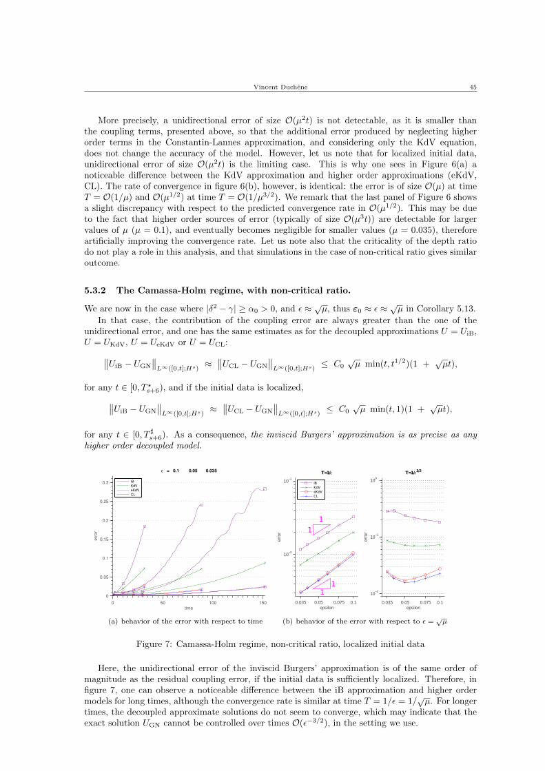
Vincent Duchene 45

More precisely, a unidirectional error of size O(µ2t) is not detectable, as it is smaller thanthe coupling terms, presented above, so that the additional error produced by neglecting higherorder terms in the Constantin-Lannes approximation, and considering only the KdV equation,does not change the accuracy of the model. However, let us note that for localized initial data,unidirectional error of size O(µ2t) is the limiting case. This is why one sees in Figure 6(a) anoticeable difference between the KdV approximation and higher order approximations (eKdV,CL). The rate of convergence in figure 6(b), however, is identical: the error is of size O(µ) at timeT = O(1/µ) and O(µ1/2) at time T = O(1/µ3/2). We remark that the last panel of Figure 6 showsa slight discrepancy with respect to the predicted convergence rate in O(µ1/2). This may be dueto the fact that higher order sources of error (typically of size O(µ3t)) are detectable for largervalues of µ (µ = 0.1), and eventually becomes negligible for smaller values (µ = 0.035), thereforeartificially improving the convergence rate. Let us note also that the criticality of the depth ratiodo not play a role in this analysis, and that simulations in the case of non-critical ratio gives similaroutcome.

5.3.2 The Camassa-Holm regime, with non-critical ratio.

We are now in the case where |δ2 − γ| ≥ α0 > 0, and ε ≈ √µ, thus ε0 ≈ ε ≈√µ in Corollary 5.13.

In that case, the contribution of the coupling error are always greater than the one of theunidirectional error, and one has the same estimates as for the decoupled approximations U = UiB,U = UKdV, U = UeKdV or U = UCL:∥∥UiB − UGN

∥∥L∞([0,t];Hs)


∥∥L∞([0,t];Hs)

≤ C0√µ min(t, t1/2)(1 +

√µt),

for any t ∈ [0, T ?s+6), and if the initial data is localized,∥∥UiB − UGN

∥∥L∞([0,t];Hs)


∥∥L∞([0,t];Hs)

≤ C0√µ min(t, 1)(1 +

√µt),

for any t ∈ [0, T ]s+6). As a consequence, the inviscid Burgers’ approximation is as precise as anyhigher order decoupled model.

0 50 100 150

0

0.05

0.1

0.15

0.2

0.25

0.3

time

err

or

ε = 0.1 0.05 0.035

iB

KdV

eKdV

CL


0.035 0.05 0.075 0.1

10−2

10−1

epsilon

error

T=1/ε

iBKdVeKdVCL

0.035 0.05 0.075 0.1

10−2

10−1

100

epsilon

error

T=1/ε3/2

1

1

11


Figure 7: Camassa-Holm regime, non-critical ratio, localized initial data

Here, the unidirectional error of the inviscid Burgers’ approximation is of the same order ofmagnitude as the residual coupling error, if the initial data is sufficiently localized. Therefore, infigure 7, one can observe a noticeable difference between the iB approximation and higher ordermodels for long times, although the convergence rate is similar at time T = 1/ε = 1/

√µ. For longer

times, the decoupled approximate solutions do not seem to converge, which may indicate that theexact solution UGN cannot be controlled over times O(ε−3/2), in the setting we use.


5.3.3 The Camassa-Holm regime, critical case.

Now let us assume that δ2 − γ = O(√µ), and ε ≈ √µ, so that ε0 ≈ µ in Corollary 5.13.

We recall that T ? and T ] are known to exist and to be of size T = O(1/max(ε, µ)) = O(µ−1/2),as a result of Proposition 3.1. Over such time, the unidirectional error in the eKdV model is smallerthan the coupling errors: one has for both U = UeKdV and U = UCL,∥∥UeKdV − UGN

∥∥L∞([0,t];Hs)


∥∥L∞([0,t];Hs)

≤ C0 µ min(t, t1/2),

for any t ∈ [0, T ?s+6) if T ? = O(µ−1/2). If moreover, the initial data is localized, then∥∥UeKdV − UGN

∥∥L∞([0,t];Hs)


∥∥L∞([0,t];Hs)

≤ C0 µ min(t, 1),

for any t ∈ [0, T ]s+6) if T ] = O(µ−1/2). The accuracy of both eKdV and CL approximations are

of size O(µ3/4) at time T = O(µ−1/2) = O(ε−1), or improved to size O(µ) if the initial data issufficiently localized. The accuracy of the KdV and iB approximation is of size O(µ1/2) at the lattertime.

However, if one looks at longer times, then the picture is different. In our simulations, we lookedat times up to T = O(ε−3/2) = O(µ−3/4). At that time, the localization in space of the initialdata plays an important role. If the initial data is non-localized in space, then contribution of thecoupling terms are predicted to be greater than the unidirectional error of the eKdV approximation:the secular coupling error is dominant up to T = O(µ−1) (µ

√t ≥ µ3/2t), after what the residual

coupling term is dominant (µ2t3/2 ≥ µ3/2t for t ≥ µ−1). Thus the eKdV approximation is predictedto be as precise as the CL approximation in the Camassa-Holm regime and if the initial data isnon-localized in space, even if the depth ratio is critical.

On the contrary, if the initial data is localized, then the unidirectional error is dominant: µ3/2t ≥µ(1 + µt) for any t ≥ µ−1/2. This leads, at time T = O(µ−3/4), to an error of size O(µ) for theCL approximation, and of size O(µ3/4) for the eKdV approximation. If the initial data is localized,then the CL approximation is substantially more accurate than the eKdV approximation after verylong time, in the Camassa-Holm regime with critical depth ratio.

The difference between localized and non-localized initial data can be clearly seen when com-paring Figure 8 and Figure 9. The fact the convergence rate of our numerical simulations fit thepredictions of Corollary 3.1, even for times which are out of the scope of our rigorous results, giveshope to extend the validity of the CL approximation to such times, where it becomes more precisethan lower order approximations.

0 50 100 150

0

0.5

1

1.5

2

2.5

x 10−3

time

err

or

ε = 0.1 0.05 0.035

eKdV

CL


0.035 0.05 0.075 0.1

10−3

10−2

epsilon

error

T=1/ε

eKdVCL

0.035 0.05 0.075 0.1

10−3

10−2

epsilon

error

T=1/ε3/2

eKdVCL

1

2

1

2


Figure 8: Camassa-Holm regime, critical ratio, localized initial data

Vincent Duchene 47

0 50 100 150

0

0.005

0.01

0.015

0.02

0.025

0.03

0.035

0.04

time

err

or

ε = 0.1 0.05 0.035

eKdV

CL


0.035 0.05 0.075 0.1

10−3

10−2

10−1

epsilon

error

T=1/ε

eKdVCL

0.035 0.05 0.075 0.1

10−2

10−1

epsilon

error

T=1/ε3/2

eKdVCL

1

3/2 1

5/4


Figure 9: Camassa-Holm regime, critical ratio, non-localized initial data

References

[1] M. A. Alejo. Well-posedness and stability results for the Gardner equation. NoDEA NonlinearDifferential Equations Appl., 19(4):503–520, 2012.

[2] B. Alvarez-Samaniego and D. Lannes. Large time existence for 3D water-waves and asymp-totics. Invent. Math., 171(3):485–541, 2008.

[3] B. Alvarez-Samaniego and D. Lannes. A Nash-Moser theorem for singular evolution equations.Application to the Serre and Green-Naghdi equations. Indiana Univ. Math. J., 57(1):97–131,2008.

[4] R. Barros and S. Gavrilyuk. Dispersive nonlinear waves in two-layer flows with free surface. II.Large amplitude solitary waves embedded into the continuous spectrum. Stud. Appl. Math.,119(3):213–251, 2007.

[5] R. Barros, S. L. Gavrilyuk, and V. M. Teshukov. Dispersive nonlinear waves in two-layer flowswith free surface. I. Model derivation and general properties. Stud. Appl. Math., 119(3):191–211, 2007.

[6] T. B. Benjamin, J. L. Bona, and J. J. Mahony. Model equations for long waves in nonlineardispersive systems. Philos. Trans. Roy. Soc. London Ser. A, 272(1220):47–78, 1972.

[7] J. L. Bona, M. Chen, and J.-C. Saut. Boussinesq equations and other systems for small-amplitude long waves in nonlinear dispersive media. I. Derivation and linear theory. J. Non-linear Sci., 12(4):283–318, 2002.

[8] J. L. Bona, T. Colin, and D. Lannes. Long wave approximations for water waves. Arch. Ration.Mech. Anal., 178(3):373–410, 2005.

[9] J. L. Bona, D. Lannes, and J.-C. Saut. Asymptotic models for internal waves. J. Math. PuresAppl. (9), 89(6):538–566, 2008.

[10] J. L. Bona and J.-C. Saut. Dispersive blowup of solutions of generalized Korteweg-de Vriesequations. J. Differential Equations, 103(1):3–57, 1993.

[11] J. L. Bona and R. Smith. The initial-value problem for the Korteweg-de Vries equation. Philos.Trans. Roy. Soc. London Ser. A, 278(1287):555–601, 1975.

[12] J. Boussinesq. Theorie de l’intumescence liquide appelee onde solitaire ou de translation sepropageant dans un canal rectangulaire. C.R. Acad. Sci. Paris Ser. A-B, 72:755–759, 1871.


[13] L. Brandolese. Breakdown for the Camassa-Holm equation using decay criteria and persistencein weighted spaces. Int. Math. Res. Not. IMRN, rnr218:1–21, 2011.

[14] R. Camassa and D. D. Holm. An integrable shallow water equation with peaked solitons. Phys.Rev. Lett., 71(11):1661–1664, 1993.

[15] X. Carvajal Paredes and P. Gamboa Romero. Persistence of solutions to nonlinear evolutionequations in weighted Sobolev spaces. Electron. J. Differential Equations, pages No. 169, 10,2010.

[16] W. Choi and R. Camassa. Weakly nonlinear internal waves in a two-fluid system. J. FluidMech., 313:83–103, 1996.

[17] W. Choi and R. Camassa. Fully nonlinear internal waves in a two-fluid system. J. Fluid Mech.,396:1–36, 1999.

[18] J. Colliander, M. Keel, G. Staffilani, H. Takaoka, and T. Tao. Sharp global well-posedness forKdV and modified KdV on R and T. J. Amer. Math. Soc., 16(3):705–749 (electronic), 2003.

[19] A. Constantin. On the scattering problem for the Camassa-Holm equation. R. Soc. Lond.Proc. Ser. A Math. Phys. Eng. Sci., 457(2008):953–970, 2001.

[20] A. Constantin and D. Lannes. The hydrodynamical relevance of the Camassa-Holm andDegasperis-Procesi equations. Arch. Ration. Mech. Anal., 192(1):165–186, 2009.

[21] W. Craig, P. Guyenne, and H. Kalisch. Hamiltonian long-wave expansions for free surfacesand interfaces. Comm. Pure Appl. Math., 58(12):1587–1641, 2005.

[22] W. Craig and C. Sulem. Numerical simulation of gravity waves. J. Comput. Phys., 108(1):73–83, 1993.

[23] V. D. Djordjevic and L. G. Redekopp. The fission and disintegration of internal solitary wavesmoving over two-dimensional topography. J. Phys. Oceanogr., 8(6):1016–1024, 1978.

[24] V. Duchene. Asymptotic shallow water models for internal waves in a two-fluid system with afree surface. SIAM J. Math. Anal., 42(5):2229–2260, 2010.

[25] V. Duchene. Boussinesq/Boussinesq systems for internal waves with a free surface, and theKdV approximation. M2AN Math. Model. Numer. Anal., 46:145–185, 2011.

[26] H. R. Dullin, G. A. Gottwald, and D. D. Holm. Camassa-Holm, Korteweg-de Vries-5 and otherasymptotically equivalent equations for shallow water waves. Fluid Dynam. Res., 33(1-2):73–95, 2003. In memoriam Prof. Philip Gerald Drazin 1934–2002.

[27] A. S. Fokas. On a class of physically important integrable equations. Phys. D, 87(1-4):145–150,1995.

[28] A. S. Fokas and Q. M. Liu. Asymptotic integrability of water waves. Phys. Rev. Lett.,77(12):2347–2351, 1996.

[29] J. Ginibre and Y. Tsutsumi. Uniqueness of solutions for the generalized Korteweg-de Vriesequation. SIAM J. Math. Anal., 20(6):1388–1425, 1989.

[30] A. E. Green and P. M. Naghdi. A derivation of equations for wave propagation in water ofvariable depth. J. Fluid Mech., 78(02):237–246, 1976.

[31] R. Grimshaw. Internal solitary waves. In Advances in fluid mechanics V, volume 40 of Adv.Fluid Mech., pages 209–218. WIT Press, Southampton, 2004.

[32] R. Grimshaw, E. Pelinovsky, and O. Poloukhina. Higher-order korteweg-de vries models forinternal solitary waves in a stratified shear flow with a free surface. Nonlinear ProcessesGeophys., 9:221–235, 2002.

Vincent Duchene 49

[33] K. R. Helfrich and W. K. Melville. Long nonlinear internal waves. In Annual review of fluidmechanics. Vol. 38, volume 38 of Annu. Rev. Fluid Mech., pages 395–425. Annual Reviews,Palo Alto, CA, 2006.

[34] K. R. Helfrich, W. K. Melville, and J. W. Miles. On interfacial solitary waves over slowlyvarying topography. J. Fluid Mech., 149:305–317, 1984.

[35] R. J. Iorio, Jr. KdV, BO and friends in weighted Sobolev spaces. In Functional-analytic methodsfor partial differential equations (Tokyo, 1989), volume 1450 of Lecture Notes in Math., pages104–121. Springer, Berlin, 1990.

[36] S. Israwi. Large time existence for 1d Green-Naghdi equations. Nonlinear Analysis: Theory,Methods & Applications, 74(1):81–93, 2011.

[37] R. S. Johnson. Camassa-Holm, Korteweg-de Vries and related models for water waves. J.Fluid Mech., 455:63–82, 2002.

[38] T. Kakutani and N. Yamasaki. Solitary waves on a two-layer fluid. J. Phys. Soc. Japan,45(2):674–679, 1978.

[39] T. Kano and T. Nishida. A mathematical justification for Korteweg-de Vries equation andBoussinesq equation of water surface waves. Osaka J. Math., 23(2):389–413, 1986.

[40] T. Kato. The Cauchy problem for quasi-linear symmetric hyperbolic systems. Arch. RationalMech. Anal., 58(3):181–205, 1975.

[41] T. Kato. On the Cauchy problem for the (generalized) Korteweg-de Vries equation. In Studiesin applied mathematics, volume 8 of Adv. Math. Suppl. Stud., pages 93–128. Academic Press,New York, 1983.

[42] C. E. Kenig and G. Ponce and L. Vega. Well-posedness and scattering results for the generalizedKorteweg-de Vries equation via the contraction principle. Comm. Pure Appl. Math., 46:527–620, 1993.

[43] C. G. Koop and G. Butler. An investigation of internal solitary waves in a two-fluid system.J. Fluid Mech., 112:225–251, 1981.

[44] D. J. Korteweg and G. De Vries. On the change of form of long waves advancing in a rectangularcanal, and on a new type of long stationary waves. Philos. Mag., 5(39):422–443, 1895.

[45] D. Lannes. Secular growth estimates for hyperbolic systems. J. Differential Equations,190(2):466–503, 2003.

[46] D. Lannes. A stability criterion for two-fluid interfaces and applications. Arxiv preprint:1005.4565, 2010.

[47] D. Lannes. The water waves problem: mathematical analysis and asymptotics. To appear inMathematical Surveys and Monographs (AMS).

[48] Y. A. Li. A shallow-water approximation to the full water wave problem. Comm. Pure Appl.Math., 59(9):1225–1285, 2006.

[49] H. Michallet and E. Barthelemy. Experimental study of interfacial solitary waves. J. FluidMech., 366:159–177, 1998.

[50] J. W. Miles. On internal solitary waves. II. Tellus, 33(4):397–401, 1981.

[51] J. Nahas. A decay property of solutions to the k-generalized KdV equation. Arxiv preprint:1010.5001, 2010.


[52] J. Nahas and G. Ponce. On the persistence properties of solutions of nonlinear dispersiveequations in weighted Sobolev spaces. In Harmonic analysis and nonlinear partial differentialequations, RIMS Kokyuroku Bessatsu, B26, pages 23–36. Res. Inst. Math. Sci. (RIMS), Kyoto,2011.

[53] L. A. Ostrovsky and J. Grue. Evolution equations for strongly nonlinear internal waves. Phys.Fluids, 15(10):2934–2948, 2003.

[54] L. A. Ostrovsky and Y. A. Stepanyants. Do internal solitons exist in the ocean? Rev. Geophys.,27(3):293–310, 1989.

[55] L. A. Ostrovsky and Y. A. Stepanyants. Internal solitons in laboratory experiments: compar-ison with theoretical models. Chaos, 15(3):037111,1–28, 2005.

[56] D. H. Peregrine. Calculations of the development of an undular bore. J. Fluid. Mech.,25(2):321–330, 1966.

[57] T. Sakai and L. G. Redekopp. Models for strongly-nonlinear evolution of long internal wavesin a two-layer stratification. Nonlinear Processes in Geophysics, 14(1):31–47, 2007.

[58] J.-C. Saut and L. Xu. The Cauchy problem on large time for surface waves Boussinesq systems.J. Math. Pures Appl. (9), 97(6):635–662, 2012.

[59] G. Schneider and C. E. Wayne. The long-wave limit for the water wave problem. I. The caseof zero surface tension. Comm. Pure Appl. Math., 53(12):1475–1535, 2000.

[60] L. F. Shampine and M. W. Reichelt. The MATLAB ODE suite. SIAM J. Sci. Comput.,18(1):1–22, 1997. Dedicated to C. William Gear on the occasion of his 60th birthday.

[61] M. E. Taylor. Partial differential equations. I Basic theory, volume 23 of Texts in AppliedMathematics. Springer-Verlag, New York, 1996.

[62] L. N. Trefethen. Spectral methods in MATLAB, volume 10 of Software, Environments, andTools. Society for Industrial and Applied Mathematics (SIAM), Philadelphia, PA, 2000.

[63] O. P. Vera Villagran. Existence and uniqueness for a nonlinear dispersive equation. Divulg.Mat., 10(2):131–148, 2002.

[64] G. B. Whitham. Linear and nonlinear waves. Pure and Applied Mathematics (New York).John Wiley & Sons Inc., New York, 1999. Reprint of the 1974 original, A Wiley-IntersciencePublication.

[65] J. D. Wright. Corrections to the KdV approximation for water waves. SIAM J. Math. Anal.,37(4):1161–1206 (electronic), 2005.

[66] L. Xu. Intermediate long wave systems for internal waves. Nonlinearity, 25(3):597–640, 2012.

[67] V. E. Zakharov. Stability of periodic waves of finite amplitude on the surface of a deep fluid.J. Appl. Mech. Tech. Phys., 9:190–194, 1968.

Documents

Decoupled and unidirectional asymptotic models for the ... · PDF fileDecoupled and unidirectional asymptotic models for the propagation of internal waves Vincent Duch^ene December