Deconvolution of Azimuthal Mode Detection Measurements

NLR – Netherlands Aerospace Centre

CUSTOMER: Netherlands Aerospace Centre

Deconvolution of Azimuthal Mode Detection Measurements

NLR-TP-2017-306 | December 2017

Netherlands Aerospace Centre

NLR is a leading international research centre for

aerospace. Bolstered by its multidisciplinary expertise

and unrivalled research facilities, NLR provides innovative

and integral solutions for the complex challenges in the

aerospace sector.

For more information visit: www.nlr.nl

NLR's activities span the full spectrum of Research

Development Test & Evaluation (RDT & E). Given NLR's

specialist knowledge and facilities, companies turn to NLR

for validation, verification, qualification, simulation and

evaluation. NLR thereby bridges the gap between research

and practical applications, while working for both

government and industry at home and abroad.

NLR stands for practical and innovative solutions, technical

expertise and a long-term design vision. This allows NLR's

cutting edge technology to find its way into successful

aerospace programs of OEMs, including Airbus, Embraer

and Pilatus. NLR contributes to (military) programs, such

as ESA's IXV re-entry vehicle, the F-35, the Apache

helicopter, and European programs, including SESAR and

Clean Sky 2.

Founded in 1919, and employing some 650 people, NLR

achieved a turnover of 71 million euros in 2016, of which

three-quarters derived from contract research, and the

remaining from government funds.

UNCLASSIFIED

EXECUTIVE SUMMARY

Problem area

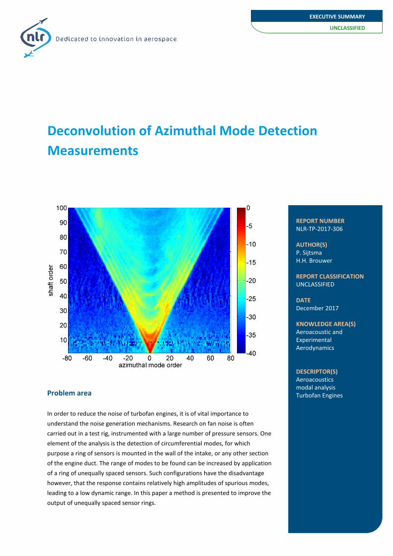
In order to reduce the noise of turbofan engines, it is of vital importance to understand the noise generation mechanisms. Research on fan noise is often carried out in a test rig, instrumented with a large number of pressure sensors. One element of the analysis is the detection of circumferential modes, for which purpose a ring of sensors is mounted in the wall of the intake, or any other section of the engine duct. The range of modes to be found can be increased by application of a ring of unequally spaced sensors. Such configurations have the disadvantage however, that the response contains relatively high amplitudes of spurious modes, leading to a low dynamic range. In this paper a method is presented to improve the output of unequally spaced sensor rings.


REPORT NUMBER NLR-TP-2017-306 AUTHOR(S) P. Sijtsma H.H. Brouwer REPORT CLASSIFICATION UNCLASSIFIED DATE December 2017 KNOWLEDGE AREA(S) Aeroacoustic and Experimental Aerodynamics DESCRIPTOR(S) Aeroacoustics modal analysis Turbofan Engines

UNCLASSIFIED

EXECUTIVE SUMMARY

GENERAL NOTE This report is based on a presentation held at the 23rd AIAA/CEAS Aeroacoustics Conference, Denver, Colorado, USA, 5-9 June 2017.

NLR

Anthony Fokkerweg 2

1059 CM Amsterdam

p ) +31 88 511 3113 f ) +31 88 511 3210

e ) [email protected] i ) www.nlr.nl

Description of work

A deconvolution strategy has been derived for increasing the dynamic range of unequally spaced sensor rings. It starts with separating the measured sound into shaft tones and broadband noise. For broadband noise modes, a standard Non-Negative Least Squares solver appeared to be a perfect deconvolution tool. For shaft tones a Matching Pursuit approach is proposed, taking advantage of the sparsity of dominant modes.

Results and conclusions

The deconvolution methods were applied to mode detection measurements in an AneCom fan rig. An increase in dynamic range of typically 10 to 15 dB was found. The following quality checks were made: a) For broadband noise the summed mode powers were compared with the average auto-powers. The agreement was within 0.1 dB. b) For tones the mode amplitudes obtained with MP were used to reconstruct the transducer data, which were compared to the actual measurements. Excellent agreement was found.

Applicability

The method presented can be used to accurately assess the modes of both tonal and broadband noise in a turbofan test rig. This information is necessary to understand the noise generation mechanisms and to design quieter engines.

NLR - Netherlands Aerospace Centre

AUTHOR(S):

P. Sijtsma PSA3 H.H. Brouwer NLR



CUSTOMER: Netherlands Aerospace Centre

2

December 2017 | NLR-TP-2017-306

CUSTOMER Netherlands Aerospace Centre

CONTRACT NUMBER -----

OWNER Netherlands Aerospace Centre

DIVISION NLR Aerospace Vehicles

DISTRIBUTION Unlimited

CLASSIFICATION OF TITLE UNCLASSIFIED

APPROVED BY :

AUTHOR REVIEWER MANAGING DEPARTMENT P. SijtsmaH. Brouwer

K. Lammers J. Hakkaart

DATE DATE DATE

This report is based on a presentation held at the 23rd AIAA/CEAS Aeroacoustics Conference, Denver, Colorado, USA, 5-9 June 2017.

The contents of this report may be cited on condition that full credit is given to NLR and the authors. This publication has been refereed by the Advisory Committee AEROSPACE VEHICLES (AV).

suurdj

New Stamp

3


Contents

Summary 5

Nomenclature 5

I. Introduction 6

II. Mathematical description 6 A. Beamforming basics 7 B. Tonal sound and broadband noise 8 C. Deconvolution of broadband noise modes 8 D. Deconvolution of tonal modes 9

III. Application to fan rig mode detection data 10 A. Broadband noise 10 B. Shaft tones 10

IV. Discussion 11

V. Conclusions 11

Appendix: Incoherence of broadband noise modes in engine ducts 12

Acknowledgments 12

References 12

Figures 13

4


This page is intentionally left blank.

5


1 American Institute of Aeronautics and Astronautics


Pieter Sijtsma* PSA3, 8091 AV Wezep, The Netherlands

Harry Brouwer† Netherlands Aerospace Centre NLR, 1059 CM Amsterdam, The Netherlands

Unequally spaced transducer rings make it possible to extend the range of detectable azimuthal modes. The other side of the coin is that the response of the mode detection algorithm to a single mode is distributed over all detectable modes, similarly to the Point Spread Function of Conventional Beamforming with microphone arrays. With multiple modes the response patterns interfere, leading to a relatively high “noise floor” of spurious modes in the detected mode spectrum, in other words, to a low dynamic range. In this paper a deconvolution strategy is proposed for increasing this dynamic range. It starts with separating the measured sound into shaft tones and broadband noise. For broadband noise modes, a standard Non-Negative Least Squares solver appeared to be a perfect deconvolution tool. For shaft tones a Matching Pursuit approach is proposed, taking advantage of the sparsity of dominant modes. The deconvolution methods were applied to mode detection measurements in an AneCom fan rig. An increase in dynamic range of typically 10 to 15 dB was found.

NomenclatureBPF Blade Passing Frequency CB Conventional Beamforming CSM Cross-Spectral Matrix DFT Direct Fourier Transform MCSM Mode Cross-Spectral Matrix MP Matching Pursuit NNLS Non-Negative Least Squares PSF Point Spread Function SPL Sound Pressure Level A CB Mode Cross-Spectral Matrix a CB amplitude vector

ka CB amplitude B Mode Cross-Spectral Matrix b mode amplitude vector

kb mode amplitude C Cross-Spectral Matrix G steering matrix

, kg g steering vector ,, n k ng g steering vector element

i imaginary unit J cost function j azimuthal mode order

K number of modes k azimuthal mode order N number of transducers n transducer index p pressure vector

np pressure amplitudes Q convolution matrix

kjQ Point Spread Function S convolution matrix for incoherent modes

kjS elements of S U CB mode auto-power vector

ku CB mode auto-power V mode auto-power vector

kv mode auto-power W weight matrix

kw weight vector kΠ Point Spread Function brb(.) broadband (non-periodic) dec(.) deconvolved res(.) residual sub(.) subset of detectable modes ton(.) tonal (shaft-periodic)

* Director; also at Aircraft Noise & Climate Effects, Delft University of Technology, Faculty of Aerospace Engineering, The Netherlands † Senior Scientist, Department of Helicopters & Aeroacoustics, P.O. Box 90502

6



I. Introduction ECOMPOSITION of the acoustic field into its azimuthal components can reveal valuable information about sound generating mechanisms. For that reason so-called “mode detection measurements”, aiming at performing

such decompositions, are standard tools in experimental engine noise studies with fan rigs1, static full-size engine tests2, and flight measurements3. The distribution of azimuthal (or circumferential or spinning) modes of shaft order tones provides insight in phenomena like rotor-stator interaction noise4, steady flow distortion noise5 and scattering by liner splices3. Modal information of broadband noise is useful too, for example in combination with phased array beamforming6.

Azimuthal mode measurements are typically performed with ring-shaped arrays of microphones (or pressure transducers). Such arrays don’t provide information about radial modes. These can be measured by means of radial rakes instrumented with pressure transducers7-10 or by means of a rotating axial transducer array mounted flush in the duct wall8.

The most natural array for mode detection is a ring of equally spaced transducers. Then the inversion problem that needs to be solved to obtain, at a given frequency, the amplitudes of the modes features an orthogonal matrix, which is easily inverted. The resulting modal amplitudes can be evaluated with a Direct Fourier Transform (DFT) applied to the transducer pressure amplitudes. The number of modes that can be detected is equal to the number of transducers. The Nyquist-Shannon sampling criterion implicates that the absolute mode order should be less than half the number of transducers. Aliasing occurs when higher order modes exist.

The range of modes that can be measured without aliasing can be extended by using a non-equally spaced array1. But then the inversion problem and the DFT solution are no longer equivalent. The inversion problem cannot deal with more modes than transducers, and the DFT method introduces the detection of spurious modes1.

When the analysis is restricted to tonal (shaft-periodic) sound, advantage can be taken from the fact that the sound field is usually dominated by a limited set of modes. This “sparsity” of modes has recently11,12 been exploited by applying Compressed (or Compressive) Sensing, which is a signal processing technique aiming at representing measured data with fewer samples than prescribed by the Nyquist-Shannon sampling criterion. The Compressed Sensing technique features the minimisation of the L1-norm of the vector of mode amplitudes. By application of an extended version of the Orthogonal Matching Pursuit algorithm a maximum number of dominant modes is determined accurately with a given array and after a deconvolution step the remaining mode spectrum is estimated using e.g. the DFT11. For broadband noise, of which the acoustic energy is more equally distributed over the mode orders, this may not be the most appropriate approach.

This paper proposes a strategy based on deconvolution, using lessons learned from methods that were developed over the past decade for microphone array measurements13-19, and exploiting the fact that the DFT method for azimuthal mode detection is exactly the same as Conventional Beamforming (CB) with microphone arrays20. Deconvolution methods start with CB and aim at retrieving source amplitudes using the known CB response of individual sources. In this paper, broadband noise and tonal sound are considered separately. Deconvolution of broadband noise is done with a Non-Negative Least Squares (NNLS) solver, similar to DAMAS14. For tonal sound a Matching Pursuit algorithm is used, similar to the approach followed in a few phased array deconvolution methods before19,21.

The next chapter gives a mathematical description of the proposed deconvolution strategy. In Chapter III mode detection deconvolution is applied to fan rig measurements. Chapter IV gives a brief discussion about the quality of the deconvolution data, followed by the conclusions in Chapter V.

II. Mathematical description All methods and results discussed in this paper are applied to single frequencies or frequency bins. For brevity,

the frequency-dependence is omitted in the mathematical expressions. Measured (complex) pressure amplitudes must be understood as the results of Fourier transforms applied to the time data. The terminology of acoustic beamforming is used.

D

7



A. Beamforming basics

Steering vector Beamforming starts with the definition of a steering function to describe the propagation from a potential source

to a receiver (microphone). A steering vector g consists of the steering function values of a fixed source position, evaluated at N microphone locations. Usually, in acoustic beamforming, the steering function is a Green’s function of the Helmholtz equation, but for azimuthal mode detection it is ( )exp ikθ− , where θ is the receiver’s angular position and the mode order k is the equivalent of a potential source. Thus, for the steering vector elements, we have

( )expn ng ikθ= − , (1)

where nθ is the angular position of the n-th transducer. Given a pressure vector p (vector of measured pressure amplitudes np ) and a set of K steering vectors kg , the

model assumption is that a set of mode amplitudes kb exists such that

k kk

b= ∑p g , (2)

with

( ), expk n ng ikθ= − , (3)

We can write the source model equation, Eq. (2), in condensed form: =p Gb , (4)

where b is the K-dimensional “mode amplitude vector” and G the N×K-dimensional “steering matrix”, the columns of which are the steering vectors.

Conventional Beamforming The Conventional Beamforming (CB) approach to find approximate source amplitudes ka is to determine, for

each unknown mode order separately, a best match with the measured data by minimizing:

2k kJ a= −p g . (5)

The minimum value of the cost function J is found for k ka ∗= w p , (6)

where the asterisk stands for “complex conjugate transpose” and the “weight vector” kw is given by

1k k

k k∗=w g

g g. (7)

Evaluating Eq. (6) with Eq. (3) yields

( )1

1 expN

k n nn

a p ikN

θ=

= ∑ , (8)

which is identical to the DFT expression used by Rademaker et al1. The CB expression, Eq. (6), can be written in condensed form too: ∗=a W p , (9)

where W is the N×K-dimensional “weight matrix” and a the K-dimensional “CB amplitude vector”.

Convolution By combining the source model equation, Eq. (4), and the CB expression, Eq. (9), we obtain =a Qb , (10)

in which the K×K-dimensional convolution matrix Q is defined by

∗=Q W G . (11) The challenge of deconvolution methods is to solve b from Eq. (10).

8



For equally-spaced mode detection arrays it can be derived that Q is the identity matrix, which means that CB yields the correct mode amplitudes. Otherwise, Eq. (10) describes convolution, which is the linear combination of responses of single unit modes j=b e . For the response of a unit mode order j to mode order k we have

( )k j kj k jka Q ∗= = =Qe w g . (12)

This is the so-called Point Spread Function (PSF). Evaluating kjQ with Eq. (3) yields

( )def

1

1 expN

kj n k jn

Q i k jN

θ −=

= − = Π ∑ . (13)

In general the rank of the matrix Q is smaller than its dimension and it cannot be inverted.

Ensemble averaging Estimates of the mode cross-spectral data can be obtained by multiplying the amplitude vector b with its

conjugate transpose, and averaging the results over many time blocks. With Eq. (9) the following estimate of the Mode Cross-Spectral Matrix (MCSM) is obtained:

∗ ∗ ∗ ∗= = =A aa W pp W W CW , (14)

where C is the traditional Cross-Spectral Matrix (CSM). With Eq. (4) we obtain the following convolution expression:

∗ ∗ ∗ ∗ ∗ ∗= = =A W G bb G W Q bb Q QBQ , (15)

where B is the actual MCSM. Eq. (15) is an order of magnitude more difficult to solve than Eq. (10), unless simplifying assumptions can be made for B. These will be discussed in the following section.

B. Tonal sound and broadband noise Sound in an engine duct can typically be split into a “tonal” part that is periodic with the shaft rotation and a

“broadband” non-periodic part: ton brb= +p p p . (16)

Suppose that “phase locked” Fourier transforms1 were performed, yielding “shaft order” spectra (i.e., the frequencies are multiples of the shaft rotation frequency). Then the process of averaging over many shaft revolutions yields for the CSM:

ton ton brb brb ton ton brb∗ ∗ ∗ ∗= = + = +C pp p p p p p p C . (17)

Likewise, for the MCSM we have ton ton brb

∗= +B b b B . (18) By inserting Eq. (17) into Eq. (14) we find for the estimated MCSM

( )( )ton ton brb

∗∗ ∗ ∗= +A W p W p W C W . (19)

Thus, we can split the convolution into a tonal part:

( )( ) ( )( )ton ton ton ton ton

∗ ∗∗ ∗= =A W p W p Qb Qb (20)

and a broadband part brb brb brb

∗ ∗= =A W C W QB Q . (21) The tonal part of the convolution is equivalent to

ton ton ton∗= =a W p Qb . (22)

C. Deconvolution of broadband noise modes The starting point is brb=A A , obtained by evaluating the first equality of Eq. (21), and the challenge is obtain a

better estimate for brb=B B using the convolution expression

∗=A QBQ . (23)

9



For broadband noise in an engine duct it’s reasonable to assume that modes with different orders are incoherent (see Appendix). This means that the off-diagonal terms in A and B can be set to zero, leading to

diag( ) diag( ) ∗=U Q V Q , (24) where V is the vector of actual mode auto-powers, k kkv B= , and U the vector of CB-estimated mode auto-powers,

k kku A= . We can derive: =U SV , (25)

where the K×K-dimensional matrix S is defined by

2

kj kjS Q= . (26)

When solving Eq. (25), the constraint of non-negativity needs to be put on the elements of V, being auto-powers. The problem of finding non-negative solutions of Eq. (25) is a key issue in microphone array deconvolution

methods, when the assumption of incoherent sources is made. A well-known algorithm to solve the problem is DAMAS, proposed by Brooks and Humphreys14, which features a Gauss-Seidel procedure where negative solutions are replaced by zero. Faster solution strategies were proposed by Dougherty et al., through the assumption of PSF shift-invariance13 or by using Linear Programming18.

For azimuthal mode detection, when the number of unknown sources is much smaller than a typical number of scan points used with beamforming, the standard Non-Negative Least Squares algorithm proposed by Lawson and Hanson20 can be used*. This solver, which we denote by “NNLS”, is a so-called “active set” method, in which negative solutions for kv are set to zero, similarly to DAMAS. This is a useful trick to make the solution space sparser when the number of possible modes is larger than the rank of S. The advantage of NNLS is that it always comes to an end after a finite number of iterations, whereas DAMAS doesn’t have a clear stop criterion. This also implies that the DAMAS result is not a solution to a well-defined optimization problem, in contrast to the NNLS result.

D. Deconvolution of tonal modes The starting point is now ton=a a , obtained with the first equality of Eq. (22), and the challenge is obtain a better

estimate for ton=b b using the convolution expression =a Qb . (27)

By definition, Eq. (11), the rank of Q is at most max{K,N}. Thus, if the number K of detectable modes is larger than the number N of transducers, Eq. (27) is not invertible. The NNLS trick of replacing negative results by zero doesn’t work either, as there is not a non-negativity constraint. Unlike Eq. (25), which is a real-valued system, Eq. (27) is complex-valued. In this case, a Matching Pursuit (MP) algorithm, as used in a few phased array deconvolution methods before19,21, can improve the results. The idea is as follows.

From the set of detectable modes, a subset of subK modes is considered with the largest absolute values of kb . Typically, subK is much less than N. Assuming that this set is known, we can estimate the corresponding amplitudes

kb by minimizing

2sub subJ = −a Q b . (28)

Herein, subb is a subK -dimensional vector with only the subset amplitudes, and subQ is a subK K× -dimensional matrix containing only the subset PSFs. The solution that minimises Eq. (28) is the Moore-Pennrose pseudoinverse:

( ) 1

sub sub sub sub

−∗ ∗=b Q Q Q a . (29)

Defining a “residual” CB amplitude vector by res sub sub= −a a Q b , (30)

the deconvolved amplitude vector is given by dec sub res= +a b a . (31)

The effects of convolution are then only present in the residual mode amplitudes in the resa vector.

* The Matlab implementation of the Lawson-Hanson NNLS algorithm is “lsqnonneg”.

10



The question remains how to find the subset containing the dominant modes. This can be done by the following iteration strategy in which a fixed (chosen) subset dimension, subK , is used:

Step 0. Determine a by CB, set dec =a a and start with an empty mode subset. Step 1. Define a new mode subset by the subK largest values of deca . When the new subset is the same as the

old subset, stop the iteration. Step 2. Calculate subb from Eq. (29). Step 3. Calculate resa from Eq. (30). Step 4. Calculate deca from Eq. (31). Step 5. Return to Step 1.

In this way the function J defined in eq.(28) is not only minimized with respect to the amplitude vector a, but also with respect to all possible choices for the subset. The choice of the number of subset modes, subK , can be inspired by looking at the condition numbers of the matrices sub sub

∗Q Q . These condition numbers increase with subK , but should not be too large.

The Matching Pursuit approach outlined above, featuring a fixed subK , is different from the standard “Greedy Algorithm”, which starts with sub 1K = and adds a solution at each iteration step. The procedure followed here needs less iterations and is thus faster.

III. Application to fan rig mode detection data The deconvolution techniques described in the previous chapter were applied to measurements performed in the

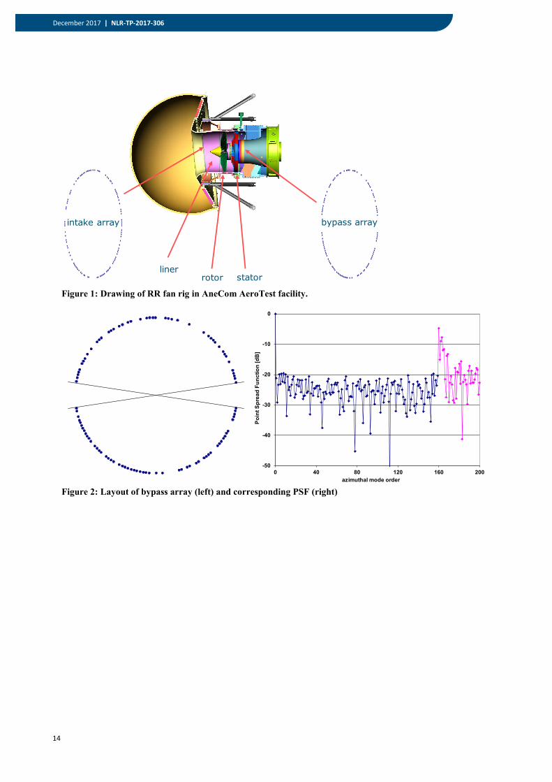
AneCom AeroTest facility on a Rolls-Royce fan rig. Figure 1 shows a drawing of the rig. The internal diameter was approximately 80 cm. Two mode detection arrays were installed. The first one was in the outer surface of the bypass duct, approximately 15 cm downstream of the 44-vanes stator. The second array was in the (drooped) intake, about 40 cm ahead of the 20-blades rotor. A liner was installed between the rotor and the array.

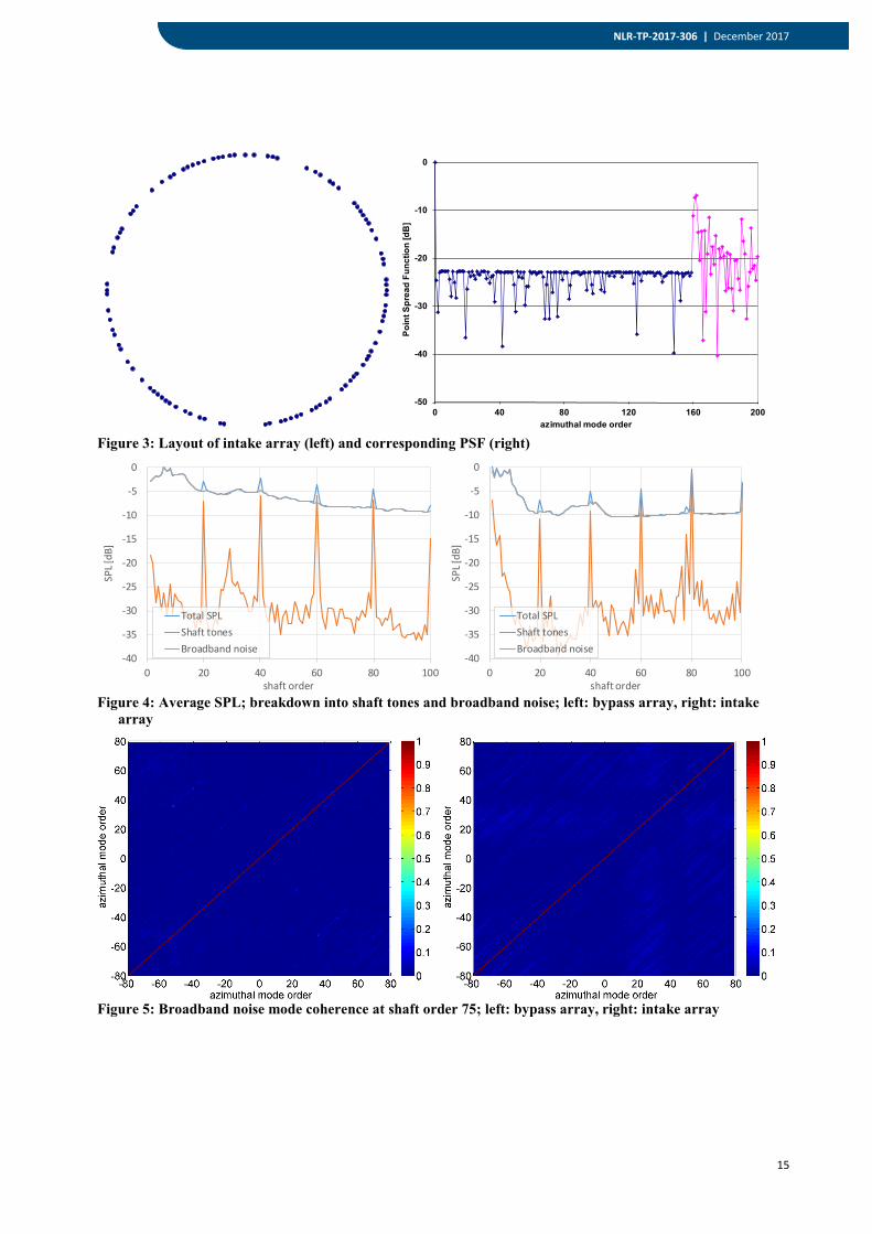
The arrays both consisted of 100N = Kulite transducers, with non-uniform layout in order to be able to detect modes in the range 80 79k− ≤ ≤ ( 160)K = . For that purpose, the maximum absolute value of kΠ , Eq. (13), was minimized for 1 1k K≤ ≤ − . The bypass array was optimized with the additional constraint of two non-accessible sectors. The layout of both arrays and their PSFs (expressed in dB) are shown in Figure 2 and Figure 3. As can be seen in the PSF images, the optimisation process led to aliasing peaks at 160k = . The dynamic range (level difference between 0Π and { }max ; 1, , 1 k k KΠ = − ) is 19.56 dB for the bypass array and 22.64 dB for the intake array.

A measurement is considered here at 60% engine speed. A breakdown of the average Sound Pressure Level (SPL) at both arrays into shaft tones and broadband noise is shown in Figure 4. Only at the Blade Passing Frequency (BPF) and higher harmonics, i.e., where the shaft orders are multiples of the number of rotor blades (20), tones have significant levels. At other shaft orders broadband noise dominates.

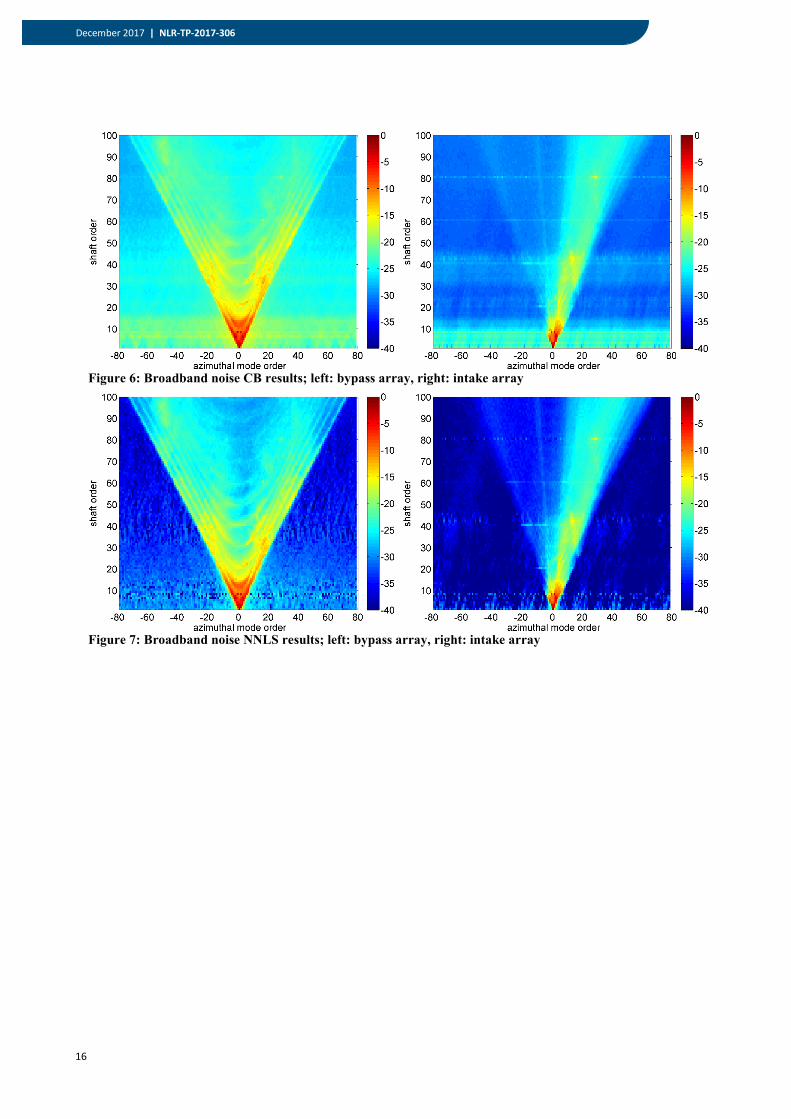
A. Broadband noise CB and NNLS were applied to broadband noise data at all shaft orders up to 100. First, the validity of the mode

incoherence, as assumed in Section II.C, was checked. This appeared to be the case, as illustrated for shaft order 75 in Figure 5. In fact, the bypass array plot (left hand side of Figure 5) vaguely shows lines at 44 and 88 shaft orders away from the diagonal. This agrees with the analysis in the Appendix.

CB results are depicted in Figure 6 and NNLS results in Figure 7. Comparing CB with NNLS, we see virtually the same mode levels in the triangle of propagating modes. But outside the triangle, the NNLS levels are typically 10 dB lower. At each shaft order, the NNLS results were summed and compared with the average SPL. A maximum difference of only 0.1 dB was found, thus demonstrating the high quality of the NNLS results.

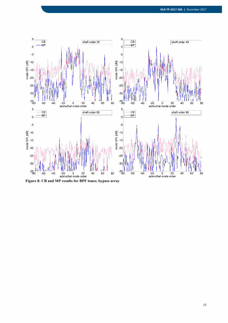
B. Shaft tones The MP method, outlined in Section II.D, was applied to the BPF tones, i.e., to shaft orders 20, 40, 60, and 80.

The iteration process was done with subsets of sub 30K = modes. For each of the 8 cases (intake and bypass) the

11



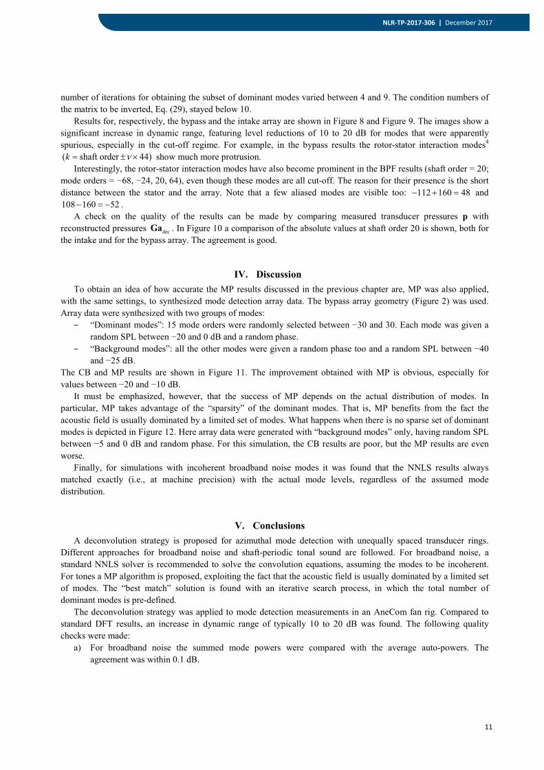
number of iterations for obtaining the subset of dominant modes varied between 4 and 9. The condition numbers of the matrix to be inverted, Eq. (29), stayed below 10.

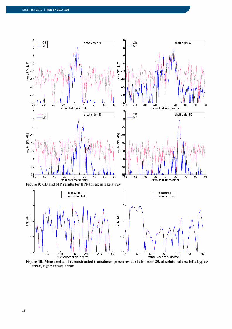
Results for, respectively, the bypass and the intake array are shown in Figure 8 and Figure 9. The images show a significant increase in dynamic range, featuring level reductions of 10 to 20 dB for modes that were apparently spurious, especially in the cut-off regime. For example, in the bypass results the rotor-stator interaction modes4 ( shaft order 44)k ν= ± × show much more protrusion.

Interestingly, the rotor-stator interaction modes have also become prominent in the BPF results (shaft order = 20; mode orders = −68, −24, 20, 64), even though these modes are all cut-off. The reason for their presence is the short distance between the stator and the array. Note that a few aliased modes are visible too: 112 160 48− + = and 108 160 52− = − .

A check on the quality of the results can be made by comparing measured transducer pressures p with reconstructed pressures decGa . In Figure 10 a comparison of the absolute values at shaft order 20 is shown, both for the intake and for the bypass array. The agreement is good.

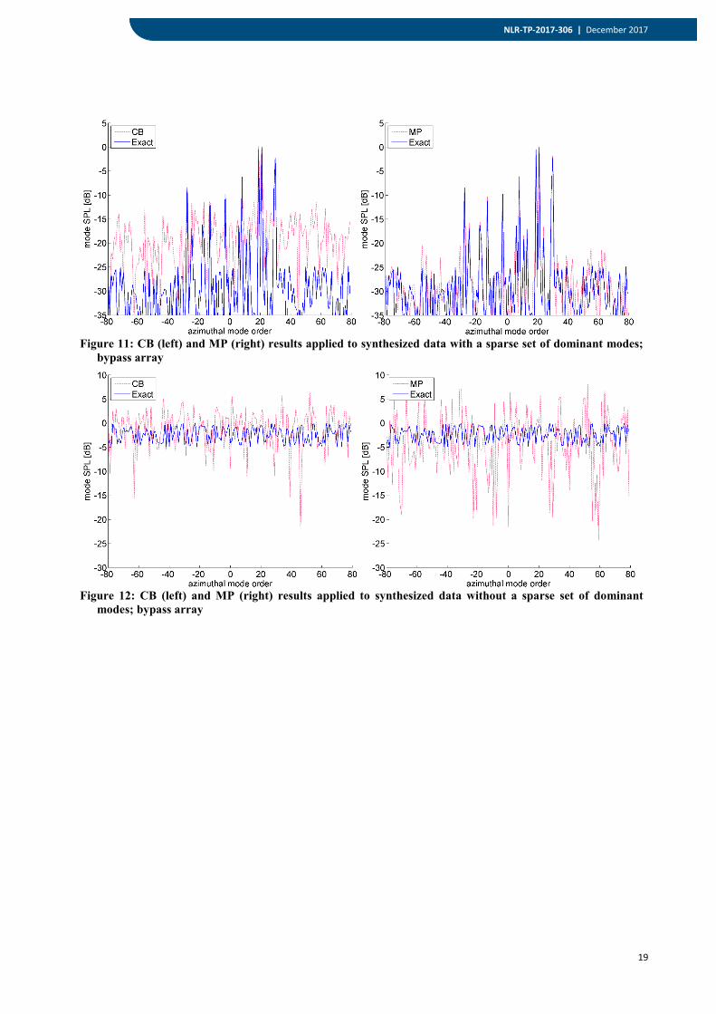
IV. Discussion To obtain an idea of how accurate the MP results discussed in the previous chapter are, MP was also applied,

with the same settings, to synthesized mode detection array data. The bypass array geometry (Figure 2) was used. Array data were synthesized with two groups of modes:

− “Dominant modes”: 15 mode orders were randomly selected between −30 and 30. Each mode was given a random SPL between −20 and 0 dB and a random phase.

− “Background modes”: all the other modes were given a random phase too and a random SPL between −40 and −25 dB.

The CB and MP results are shown in Figure 11. The improvement obtained with MP is obvious, especially for values between −20 and −10 dB.

It must be emphasized, however, that the success of MP depends on the actual distribution of modes. In particular, MP takes advantage of the “sparsity” of the dominant modes. That is, MP benefits from the fact the acoustic field is usually dominated by a limited set of modes. What happens when there is no sparse set of dominant modes is depicted in Figure 12. Here array data were generated with “background modes” only, having random SPL between −5 and 0 dB and random phase. For this simulation, the CB results are poor, but the MP results are even worse.

Finally, for simulations with incoherent broadband noise modes it was found that the NNLS results always matched exactly (i.e., at machine precision) with the actual mode levels, regardless of the assumed mode distribution.

V. Conclusions A deconvolution strategy is proposed for azimuthal mode detection with unequally spaced transducer rings.

Different approaches for broadband noise and shaft-periodic tonal sound are followed. For broadband noise, a standard NNLS solver is recommended to solve the convolution equations, assuming the modes to be incoherent. For tones a MP algorithm is proposed, exploiting the fact that the acoustic field is usually dominated by a limited set of modes. The “best match” solution is found with an iterative search process, in which the total number of dominant modes is pre-defined.

The deconvolution strategy was applied to mode detection measurements in an AneCom fan rig. Compared to standard DFT results, an increase in dynamic range of typically 10 to 20 dB was found. The following quality checks were made:

a) For broadband noise the summed mode powers were compared with the average auto-powers. The agreement was within 0.1 dB.

12



b) For tones the mode amplitudes obtained with MP were used to reconstruct the transducer data, which were compared to the actual measurements. Excellent agreement was found.

The good performance of NNLS and MP was confirmed with synthesized data.

Appendix: Incoherence of broadband noise modes in engine ducts An acoustic field due to a point source in a circular duct can be expressed as a summation of modes:

( )( ) expkk

p q ikθ λ θ ϕ= − − ∑ , (32)

Herein, q is the source amplitude, kλ are constants, and ϕ is the source angular position. In an engine duct, it can be expected that broadband noise sources are associated with blades in a blade row (e.g., a stator). Thus, groups of incoherent sources exist:

( )1

( ) expM

m k mm k

p q ikθ λ θ ϕ=

= − − ∑ ∑ , (33)

where M is the number of blades and mϕ their angular positions. Usually the blades are equally spaced, so we can write

2

mm

Mπϕ = . (34)

Thus, mode amplitudes corresponding with Eq. (33) are

1

exp 2M

k k mm

mb q ikM

λ π=

= ∑ (35)

For the mode cross-powers we have

1 1

exp 2M M

kj k j k j m nm n

km jnB b b q q iM

λ λ π∗ ∗ ∗

= =

− = = ∑∑ . (36)

Because the sources on different blades are incoherent, we obtain

( )1

exp 2M

kj k j k j m mm

mB b b q q i k jM

λ λ π∗ ∗ ∗

=

= = − ∑ . (37)

The assumption that all sources have the same, unit, strength yields

𝐵𝐵𝑘𝑘𝑘𝑘 = 𝜆𝜆𝑘𝑘𝜆𝜆𝑘𝑘∗ ∑ exp �2𝜋𝜋𝜋𝜋(𝑘𝑘 − 𝑗𝑗) 𝑚𝑚𝑀𝑀�𝑀𝑀

𝑚𝑚=1 = � 𝜆𝜆𝑘𝑘𝜆𝜆𝑘𝑘∗

exp�2𝜋𝜋𝜋𝜋(𝑘𝑘−𝑘𝑘)�−11−exp(−2𝜋𝜋𝜋𝜋(𝑘𝑘−𝑘𝑘)/𝑀𝑀)

= 0, 𝑘𝑘 − 𝑗𝑗 ≠ 𝜈𝜈𝜈𝜈

𝜆𝜆𝑘𝑘𝜆𝜆𝑘𝑘∗𝜈𝜈, 𝑘𝑘 − 𝑗𝑗 = 𝜈𝜈𝜈𝜈 (38)

with ν an integer. In other words, mode cross-powers in engine ducts are expected to be zero, unless the difference between the mode orders is a multiple of the number of blades.

Note that the analysis above ignores the presence of multiple, incoherent radial modes. This will probably reduce also the cross-powers when j k Mν= + .

Acknowledgments The fan rig measurements were performed within the EU-project PROBAND (FP6). Assystem UK Ltd is

acknowledged for providing the fan rig drawing of Figure 1.

13



References 1Rademaker, E.R., Sijtsma, P., and Tester, B.J., “Mode Detection with an Optimised Array in a Model Turbofan Engine

Intake at Varying Shaft Speeds,” AIAA Paper 2001-2181. 2Lan, J., Premo, J., Zlavog, G., Breard, C., Callender, B., and Martinez, M., “Phased Array Measurements of Full-Scale

Engine Inlet Noise,” AIAA Paper 2007-3434. 3Sarin, S.L., and Rademaker, E.R., “In-Flight Acoustic Mode Measurements in the Turbofan Engine Inlet of Fokker 100

Aircraft,” AIAA Paper 93-4414. 4Tyler, J. M., and Sofrin, T. G., “Axial Flow Compressor Noise Studies,” SAE Transactions, Vol. 70, 1962, pp. 309–332. 5Prinn, A.G., Sugimoto, R., and Astley, R.J., “The Effect of Steady Flow Distortion on Noise Propagation in Turbofan

Intakes,” AIAA Paper 2016-3028. 6Sijtsma, P., “Using Phased Array Beamforming to Identify Broadband Noise Sources in a Turbofan Engine,” International

Journal of Aeroacoustics, Vol. 9, No. 3, 2010, pp. 357-374. 7Enghardt, L., Tapken, U., Neise, W., Kennepohl, F., and Heinig, K., “Turbine Blade/Vane Interaction Noise: Acoustic Mode

Analysis Using In-Duct Sensor Rakes,” AIAA Paper 2001-2153. 8Tapken, U., Bauers, R., Neuhaus, L., Humphreys, N., Wilson, A., Stöhr, C., and Beutke, M., “A New Modular Fan Rig Noise

Test and Radial Mode Detection Capability,” AIAA Paper 2011-2897. 9Heidelberg, L., and Hall, D., “Inlet Acoustic Mode Measurements Using a Continuously Rotating Rake,” AIAA Journal of

Aircraft, Vol. 32, 1995, pp. 761-767. 10Sijtsma, P., and Orsi, H., “Azimuthal and Radial Mode Detection by a Slowly Rotating Rake,” AIAA Paper 2013-2244. 11Behn, M., Kisler, R. and Tapken, U., “Efficient Azimuthal Mode Analysis using Compressed Sensing,” AIAA Paper 2016-

3038. 12Yu, W. and Huang, X., “Compressive Sensing Duct Mode Detection Method with In-Duct Microphone Array,” AIAA Paper

2016-2765. 13Dougherty, R.P., “Extensions of DAMAS and Benefits and Limitations of Deconvolution in Beamforming,” AIAA Paper

2005-2961. 14Brooks, T.F., and Humphreys, Jr., W.M., “A Deconvolution Approach for the Mapping of Acoustic Sources (DAMAS).

Determined from Phased Microphone Array,” Journal of Sound and Vibration, Vol. 294 (4-5), 2006, pp. 856-879. 15Brooks, T.F., and Humphreys, Jr., W.M., “Extension of DAMAS Phased Array Processing for Spatial Coherence

Determination (DAMAS-C),” AIAA Paper 2006-2654. 16Sijtsma, P., “CLEAN based on Spatial Source Coherence,” International Journal of Aeroacoustics, Vol. 6, 2007, pp. 357-

374. 17Yardibi, T., Lia, J., Stoica, P., and Cattafesta III, L.N., “Sparsity Constrained Deconvolution Approaches for Acoustic Source

Mapping,” Journal of the Acoustical Society of America, Vol. 123, 2008, pp 2631–2642. 18Dougherty, R.P., and Podboy G.G., “Improved Phased Array Imaging of a Model Jet,” AIAA Paper 2009-3186. 19Padois, T., and Berry, A., “Orthogonal Matching Pursuit Applied to the Deconvolution Approach for the Mapping of

Acoustic Sources Inverse Problem,” Journal of the Acoustical Society of America, Vol. 138, 2015, pp. 3678–3685. 20Sijtsma, P., “Acoustic Beamforming for the Ranking of Aircraft Noise,” published in Accurate and Efficient Aeroacoustic

Prediction Approaches for Airframe Noise, VKI Lecture Series 2013-03, Edited by C. Schram, R. Dénos, and E. Lecomte, March 25-29, 2013.

21Högbom J.A, “Aperture Synthesis with a Non-Regular Distribution of Interferometer Baselines,” Astron. Astrophys. Suppl., Vol. 15, 1974, pp. 417-426.

22Lawson, C.L., and Hanson, R.J., Solving Least Squares Problems, SIAM, 1995.

14



Figure 1: Drawing of RR fan rig in AneCom AeroTest facility.

Figure 2: Layout of bypass array (left) and corresponding PSF (right)

rotor stator

intake array bypass array

liner

-50

-40

-30

-20

-10

0

0 40 80 120 160 200

Poin

t Spr

ead

Func

tion

[dB

]

azimuthal mode order

15



Figure 3: Layout of intake array (left) and corresponding PSF (right)

Figure 4: Average SPL; breakdown into shaft tones and broadband noise; left: bypass array, right: intake

array

Figure 5: Broadband noise mode coherence at shaft order 75; left: bypass array, right: intake array

-50

-40

-30

-20

-10

0

0 40 80 120 160 200Po

int S

prea

d Fu

nctio

n [d

B]

azimuthal mode order

-40

-35

-30

-25

-20

-15

-10

-5

0

0 20 40 60 80 100

SPL [

dB]

shaft order

Total SPLShaft tonesBroadband noise

-40

-35

-30

-25

-20

-15

-10

-5

0

0 20 40 60 80 100

SPL [

dB]

shaft order

Total SPLShaft tonesBroadband noise

16



Figure 6: Broadband noise CB results; left: bypass array, right: intake array

Figure 7: Broadband noise NNLS results; left: bypass array, right: intake array

17



Figure 8: CB and MP results for BPF tones; bypass array

18



Figure 9: CB and MP results for BPF tones; intake array

Figure 10: Measured and reconstructed transducer pressures at shaft order 20, absolute values; left: bypass

array, right: intake array

19



Figure 11: CB (left) and MP (right) results applied to synthesized data with a sparse set of dominant modes;

bypass array

Figure 12: CB (left) and MP (right) results applied to synthesized data without a sparse set of dominant

modes; bypass array

20


This page is intentionally left blank.

NLR

Anthony Fokkerweg 2 1059 CM Amsterdam, The Netherlands p ) +31 88 511 3113 f ) +31 88 511 3210 e ) [email protected] i ) www.nlr.nl

Documents

Deconvolution of Azimuthal Mode Detection Measurements