DECONVOLUTION ALGORITHMS FOR

FLUORESCENCE AND ELECTRON

MICROSCOPY

by

Siddharth Shah

A dissertation submitted in partial fulfillmentof the requirements for the degree of

Doctor of Philosophy(Biomedical Engineering)

in The University of Michigan2006

Doctoral Committee:

Professor Andrew E. Yagle, ChairProfessor Paul L. CarsonProfessor Jeffrey A. FesslerAssociate Professor Mary-Ann MycekAssociate Professor Douglas C. Noll

c© Siddharth Shah 2006All Rights Reserved

ACKNOWLEDGEMENTS

This work has been possible only due to the support of several faculty, family

members and friends. First, I would like to thank my adviser Andrew Yagle for

the support and guidance when I needed them most and for supporting my decision

to work toward my thesis at UCSF. I would like to thank John Sedat and David

Agard for their tremendrous generosity in letting me work in their microscopy labs

for a year. I also thank my committee members Mary-Ann Mycek, Jeffrey Fessler,

Douglas Noll and Paul Carson for their insights and guidance. I want to thank

Michelle Young for being a wonderful person to work with.

I am grateful to my colleagues Erik Hom, Sebastian Haase, Shawn Zheng, John

Lyle and Justin Kollman who helped me in key ways on the electron microscopy

projects. Last, I want to thank my family and friends. My brother, Ashwin and

sister-in-law Indrayani gave me tremendous moral support, encouragement and most

importantly fed me tasty Indian dishes which I by no means can cook ! My par-

ents must be thanked for their support and faith in me when the chips were down.

My friends Kurt Christensen, Ken Garber, Josh Hoskins, Rajeeva Kumar and Neal

Patwari helped me at various stages of my PhD. To them, a hearty thanks !

ii

TABLE OF CONTENTS

ACKNOWLEDGEMENTS . . . . . . . . . . . . . . . . . . . . . . . . . . . . . . . . . . ii

LIST OF FIGURES . . . . . . . . . . . . . . . . . . . . . . . . . . . . . . . . . . . . . . vii

LIST OF TABLES . . . . . . . . . . . . . . . . . . . . . . . . . . . . . . . . . . . . . . . xi

CHAPTER

I. Introduction . . . . . . . . . . . . . . . . . . . . . . . . . . . . . . . . . . . . . . . 1

1.1 Problem Overview . . . . . . . . . . . . . . . . . . . . . . . . . . . . . . . . . 21.2 Previous Work . . . . . . . . . . . . . . . . . . . . . . . . . . . . . . . . . . . 3

1.2.1 Optical Microscopy . . . . . . . . . . . . . . . . . . . . . . . . . . . 31.2.2 Electron Microscopy . . . . . . . . . . . . . . . . . . . . . . . . . . 4

1.3 Contributions of this Thesis . . . . . . . . . . . . . . . . . . . . . . . . . . . 51.4 Organization of this Thesis . . . . . . . . . . . . . . . . . . . . . . . . . . . . 6

II. Principles of confocal and electron microscopy . . . . . . . . . . . . . . . . . 7

2.1 Introduction . . . . . . . . . . . . . . . . . . . . . . . . . . . . . . . . . . . . 82.1.1 The Confocal Microscope . . . . . . . . . . . . . . . . . . . . . . . 82.1.2 The Transmission Electron Microscope . . . . . . . . . . . . . . . . 92.1.3 Image Formation Processes in EM: A Qualitative Description . . . 11

2.2 Wave Optical Theory of Imaging . . . . . . . . . . . . . . . . . . . . . . . . . 142.3 Derivation of EM Imaging Equation . . . . . . . . . . . . . . . . . . . . . . . 16

2.3.1 Angular Deviation of Wavefront in an Electron Lens . . . . . . . . 162.3.2 Derivation of Phase Shift . . . . . . . . . . . . . . . . . . . . . . . . 172.3.3 Weak Amplitude Weak Phase Approximation . . . . . . . . . . . . 182.3.4 The Contrast Transfer Function . . . . . . . . . . . . . . . . . . . . 192.3.5 EM Imaging Equation . . . . . . . . . . . . . . . . . . . . . . . . . 21

III. Principles and approaches for the deconvolution problem . . . . . . . . . . 22

3.1 Basic Equation . . . . . . . . . . . . . . . . . . . . . . . . . . . . . . . . . . . 223.1.1 The Partial Data Problem . . . . . . . . . . . . . . . . . . . . . . . 243.1.2 The Case For Blind Deconvolution . . . . . . . . . . . . . . . . . . 243.1.3 A Brief Overview of Common Deconvolution Algorithms . . . . . . 253.1.4 Linear Methods . . . . . . . . . . . . . . . . . . . . . . . . . . . . . 253.1.5 Statistical Methods . . . . . . . . . . . . . . . . . . . . . . . . . . . 27

3.2 The Automatic Image Deconvolution Algorithm . . . . . . . . . . . . . . . . 293.2.1 AIDA Noise Model . . . . . . . . . . . . . . . . . . . . . . . . . . . 303.2.2 Data Fidelity Term . . . . . . . . . . . . . . . . . . . . . . . . . . . 31

iii

3.2.3 Regularization Term . . . . . . . . . . . . . . . . . . . . . . . . . . 313.2.4 Myopic Deconvolution . . . . . . . . . . . . . . . . . . . . . . . . . 323.2.5 Automatic Hyperparameter Estimation . . . . . . . . . . . . . . . . 34

IV. 2-D blind deconvolution of even point-spread functions from compactsupport images . . . . . . . . . . . . . . . . . . . . . . . . . . . . . . . . . . . . . 37

4.1 Introduction . . . . . . . . . . . . . . . . . . . . . . . . . . . . . . . . . . . . 374.1.1 Blind Deconvolution . . . . . . . . . . . . . . . . . . . . . . . . . . 374.1.2 Previous Work . . . . . . . . . . . . . . . . . . . . . . . . . . . . . 384.1.3 Problem Formulation . . . . . . . . . . . . . . . . . . . . . . . . . . 384.1.4 Problem Ambiguities . . . . . . . . . . . . . . . . . . . . . . . . . . 40

4.2 1-D Blind Deconvolution . . . . . . . . . . . . . . . . . . . . . . . . . . . . . 414.2.1 Formulation . . . . . . . . . . . . . . . . . . . . . . . . . . . . . . . 414.2.2 Resultant Solution . . . . . . . . . . . . . . . . . . . . . . . . . . . 414.2.3 Resultant Example . . . . . . . . . . . . . . . . . . . . . . . . . . . 424.2.4 Resultant Reformulation . . . . . . . . . . . . . . . . . . . . . . . . 43

4.3 2-D Blind Deconvolution . . . . . . . . . . . . . . . . . . . . . . . . . . . . . 444.3.1 Resultant Solution . . . . . . . . . . . . . . . . . . . . . . . . . . . 444.3.2 Resultant Example . . . . . . . . . . . . . . . . . . . . . . . . . . . 454.3.3 Fourier Decomposition . . . . . . . . . . . . . . . . . . . . . . . . . 464.3.4 Scale Factors . . . . . . . . . . . . . . . . . . . . . . . . . . . . . . 484.3.5 Fourier Example . . . . . . . . . . . . . . . . . . . . . . . . . . . . 484.3.6 Computational Savings . . . . . . . . . . . . . . . . . . . . . . . . . 49

4.4 Noisy Data Case . . . . . . . . . . . . . . . . . . . . . . . . . . . . . . . . . . 504.4.1 Formulation . . . . . . . . . . . . . . . . . . . . . . . . . . . . . . . 504.4.2 Resultant Solution . . . . . . . . . . . . . . . . . . . . . . . . . . . 514.4.3 Sufficiency Considerations . . . . . . . . . . . . . . . . . . . . . . . 524.4.4 Fourier Decomposition . . . . . . . . . . . . . . . . . . . . . . . . . 53

4.5 Noiseless Case . . . . . . . . . . . . . . . . . . . . . . . . . . . . . . . . . . . 554.5.1 Full Data Case . . . . . . . . . . . . . . . . . . . . . . . . . . . . . 554.5.2 Partial Data Case . . . . . . . . . . . . . . . . . . . . . . . . . . . . 56

4.6 Comparision of Rank-Reduction Procedures . . . . . . . . . . . . . . . . . . 584.6.1 Overview of Different Procedures . . . . . . . . . . . . . . . . . . . 584.6.2 Direct Method . . . . . . . . . . . . . . . . . . . . . . . . . . . . . 604.6.3 Fourier Decomposition Method . . . . . . . . . . . . . . . . . . . . 614.6.4 Regularization . . . . . . . . . . . . . . . . . . . . . . . . . . . . . . 624.6.5 Comparison of Direct and Fourier Decomposition Methods . . . . . 63

4.7 Conclusion . . . . . . . . . . . . . . . . . . . . . . . . . . . . . . . . . . . . . 65

V. 3-D blind deconvolution of even point-spread functions from compactsupport images . . . . . . . . . . . . . . . . . . . . . . . . . . . . . . . . . . . . . 66

5.1 Introduction . . . . . . . . . . . . . . . . . . . . . . . . . . . . . . . . . . . . 665.1.1 Problem Formulaton . . . . . . . . . . . . . . . . . . . . . . . . . . 675.1.2 Problem Ambiguities . . . . . . . . . . . . . . . . . . . . . . . . . . 68

5.2 2-D and 3-D Solution . . . . . . . . . . . . . . . . . . . . . . . . . . . . . . . 695.2.1 2-D Solution . . . . . . . . . . . . . . . . . . . . . . . . . . . . . . . 695.2.2 Fourier Decomposition in 2-D . . . . . . . . . . . . . . . . . . . . . 705.2.3 Scale Factors in 2-D . . . . . . . . . . . . . . . . . . . . . . . . . . 715.2.4 3-D Blind Deconvolution . . . . . . . . . . . . . . . . . . . . . . . . 715.2.5 Fourier Decomposition in 3-D . . . . . . . . . . . . . . . . . . . . . 725.2.6 Scale Factors in 3-D . . . . . . . . . . . . . . . . . . . . . . . . . . 735.2.7 Implementation Issues . . . . . . . . . . . . . . . . . . . . . . . . . 73

iv

5.3 Noisy Data Case . . . . . . . . . . . . . . . . . . . . . . . . . . . . . . . . . . 745.3.1 Formulation . . . . . . . . . . . . . . . . . . . . . . . . . . . . . . . 745.3.2 Resultant Solution . . . . . . . . . . . . . . . . . . . . . . . . . . . 755.3.3 Fourier Decomposition . . . . . . . . . . . . . . . . . . . . . . . . . 765.3.4 Overview of Simulations . . . . . . . . . . . . . . . . . . . . . . . . 775.3.5 Performance in the Absence of Noise . . . . . . . . . . . . . . . . . 775.3.6 Performance in Noise . . . . . . . . . . . . . . . . . . . . . . . . . . 785.3.7 Scaling Comparisons . . . . . . . . . . . . . . . . . . . . . . . . . . 785.3.8 Comparison with Lucy-Richardson Algorithm . . . . . . . . . . . . 83

5.4 Conclusions . . . . . . . . . . . . . . . . . . . . . . . . . . . . . . . . . . . . 83

VI. QUILL: A blind deconvolution algorithm for the partial data problem . . 85

6.1 Introduction . . . . . . . . . . . . . . . . . . . . . . . . . . . . . . . . . . . . 856.1.1 Overview . . . . . . . . . . . . . . . . . . . . . . . . . . . . . . . . 856.1.2 The Partial Data Problem . . . . . . . . . . . . . . . . . . . . . . . 866.1.3 New Contributions of This Paper . . . . . . . . . . . . . . . . . . . 87

6.2 Problem Definition . . . . . . . . . . . . . . . . . . . . . . . . . . . . . . . . 886.2.1 Problem Assumptions . . . . . . . . . . . . . . . . . . . . . . . . . 886.2.2 Problem Ambiguities . . . . . . . . . . . . . . . . . . . . . . . . . . 89

6.3 QUILL Image Model . . . . . . . . . . . . . . . . . . . . . . . . . . . . . . . 906.3.1 1-D Image Basis Representation . . . . . . . . . . . . . . . . . . . . 906.3.2 Specification of the QUILL model . . . . . . . . . . . . . . . . . . . 906.3.3 Examples of the QUILL Model . . . . . . . . . . . . . . . . . . . . 92

6.4 Solution to the QUILL Deconvolution Problem . . . . . . . . . . . . . . . . . 936.4.1 QUILL Image Deconvolution as 4-Channel Deconvolution . . . . . 936.4.2 2-D Bezout’s Lemma . . . . . . . . . . . . . . . . . . . . . . . . . . 966.4.3 Overall Approach . . . . . . . . . . . . . . . . . . . . . . . . . . . . 986.4.4 Implementation of QUILL on Real Data . . . . . . . . . . . . . . . 996.4.5 Implementation Issues . . . . . . . . . . . . . . . . . . . . . . . . . 1006.4.6 Stochastic Formulation . . . . . . . . . . . . . . . . . . . . . . . . . 101

6.5 Numerical Examples . . . . . . . . . . . . . . . . . . . . . . . . . . . . . . . . 1026.5.1 Real Images with Synthetic Blurring . . . . . . . . . . . . . . . . . 1026.5.2 Real Data . . . . . . . . . . . . . . . . . . . . . . . . . . . . . . . . 104

6.6 Conclusion . . . . . . . . . . . . . . . . . . . . . . . . . . . . . . . . . . . . . 106

VII. Contrast Transfer Function estimation for cryo and cryo-tomo electronmicroscopy images . . . . . . . . . . . . . . . . . . . . . . . . . . . . . . . . . . . 109

7.1 Introduction . . . . . . . . . . . . . . . . . . . . . . . . . . . . . . . . . . . . 1097.2 Theory of Image formation . . . . . . . . . . . . . . . . . . . . . . . . . . . . 111

7.2.1 Mathematical Description of Image Formation . . . . . . . . . . . . 1117.3 CTF Formula . . . . . . . . . . . . . . . . . . . . . . . . . . . . . . . . . . . 112

7.3.1 Planar EM . . . . . . . . . . . . . . . . . . . . . . . . . . . . . . . 1127.3.2 Tomographic EM . . . . . . . . . . . . . . . . . . . . . . . . . . . . 113

7.4 Algorithm for CTF Estimation . . . . . . . . . . . . . . . . . . . . . . . . . . 1147.4.1 Obtaining the Power Spectrum of the CTF . . . . . . . . . . . . . 1147.4.2 Background Fitting and Subtraction . . . . . . . . . . . . . . . . . 1157.4.3 Masking . . . . . . . . . . . . . . . . . . . . . . . . . . . . . . . . . 1177.4.4 Determination of Defocus and Astigmatism Parameters . . . . . . 1177.4.5 CTF estimation for Tomographic Micrographs . . . . . . . . . . . . 119

7.5 Results . . . . . . . . . . . . . . . . . . . . . . . . . . . . . . . . . . . . . . . 1217.5.1 Ice on Carbon Film Defocus Series Data . . . . . . . . . . . . . . . 1217.5.2 Validation of Determined Defocus Values . . . . . . . . . . . . . . . 121

v

7.5.3 Defocus Estimation of Protein in Ice . . . . . . . . . . . . . . . . . 1237.6 Estimation of CTF for Tilted and Tomographic Data . . . . . . . . . . . . . 125

7.6.1 CTF Parameter Estimation of Negatively Stained Conical Tilt Data1277.6.2 Tilted Defocus Series Experiment with Cryo-EM Data . . . . . . . 1287.6.3 Estimation of CTF on Tomographic Cryo-EM data . . . . . . . . . 129

7.7 Discussion . . . . . . . . . . . . . . . . . . . . . . . . . . . . . . . . . . . . . 131

VIII. Edge-preserving deconvolution for cryo-electron microscopy images . . . . 133

8.1 Introduction . . . . . . . . . . . . . . . . . . . . . . . . . . . . . . . . . . . . 1338.2 Theory of Image Formation and CTF Correction . . . . . . . . . . . . . . . . 135

8.2.1 Image Formation . . . . . . . . . . . . . . . . . . . . . . . . . . . . 1358.2.2 Deconvolution . . . . . . . . . . . . . . . . . . . . . . . . . . . . . . 136

8.3 Methods . . . . . . . . . . . . . . . . . . . . . . . . . . . . . . . . . . . . . . 1398.3.1 Sample Preparation and Acquisition . . . . . . . . . . . . . . . . . 1398.3.2 Image Processing of Individual Samples . . . . . . . . . . . . . . . 1408.3.3 Quantitative Analysis . . . . . . . . . . . . . . . . . . . . . . . . . 1408.3.4 Qualitative Analysis . . . . . . . . . . . . . . . . . . . . . . . . . . 142

8.4 Results . . . . . . . . . . . . . . . . . . . . . . . . . . . . . . . . . . . . . . . 1428.4.1 Analysis of Phase Residual Error . . . . . . . . . . . . . . . . . . . 1428.4.2 Visual Analysis of Data . . . . . . . . . . . . . . . . . . . . . . . . 143

8.5 Discussion . . . . . . . . . . . . . . . . . . . . . . . . . . . . . . . . . . . . . 145

IX. Conclusion . . . . . . . . . . . . . . . . . . . . . . . . . . . . . . . . . . . . . . . . 148

9.1 Current State of the Algorithms . . . . . . . . . . . . . . . . . . . . . . . . . 1499.1.1 Blind Even-PSF Deconvolution . . . . . . . . . . . . . . . . . . . . 1499.1.2 Blind Deconvolution using QUILL . . . . . . . . . . . . . . . . . . 1509.1.3 Contrast Transfer Function (CTF) Estimation Algorithm . . . . . 1509.1.4 Deconvolution of EM Images using the edge-preservation Algorithm 151

9.2 Future Work . . . . . . . . . . . . . . . . . . . . . . . . . . . . . . . . . . . . 1529.2.1 Deployment of Blind Deconvolution Algorithms for Fluorescence

Microscopy Applications . . . . . . . . . . . . . . . . . . . . . . . . 1529.2.2 Choice of a Different Regularizer for QUILL Algorithm . . . . . . . 1529.2.3 Improvements and Extensions to CTF Estimation Algorithm . . . 1529.2.4 Improvements to the Edge-Preserving Deconvolution Algorithm . . 153

APPENDICES . . . . . . . . . . . . . . . . . . . . . . . . . . . . . . . . . . . . . . . . . . 155

BIBLIOGRAPHY . . . . . . . . . . . . . . . . . . . . . . . . . . . . . . . . . . . . . . . . 158

vi

LIST OF FIGURES

Figure

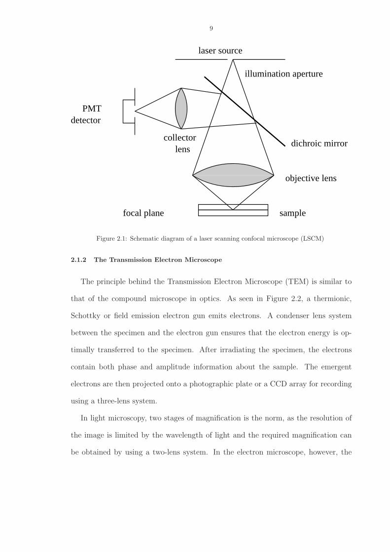
2.1 Schematic diagram of a laser scanning confocal microscope (LSCM) . . . . . . . . 9

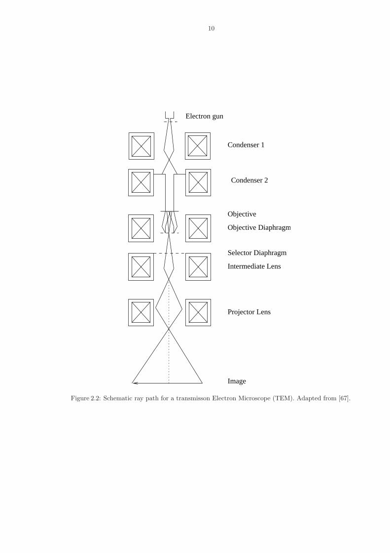
2.2 Schematic ray path for a transmisson Electron Microscope (TEM). Adapted from[67]. . . . . . . . . . . . . . . . . . . . . . . . . . . . . . . . . . . . . . . . . . . . . 10

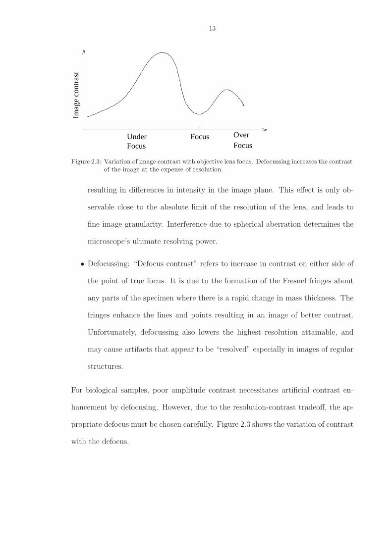
2.3 Variation of image contrast with objective lens focus. Defocussing increases thecontrast of the image at the expense of resolution. . . . . . . . . . . . . . . . . . . 13

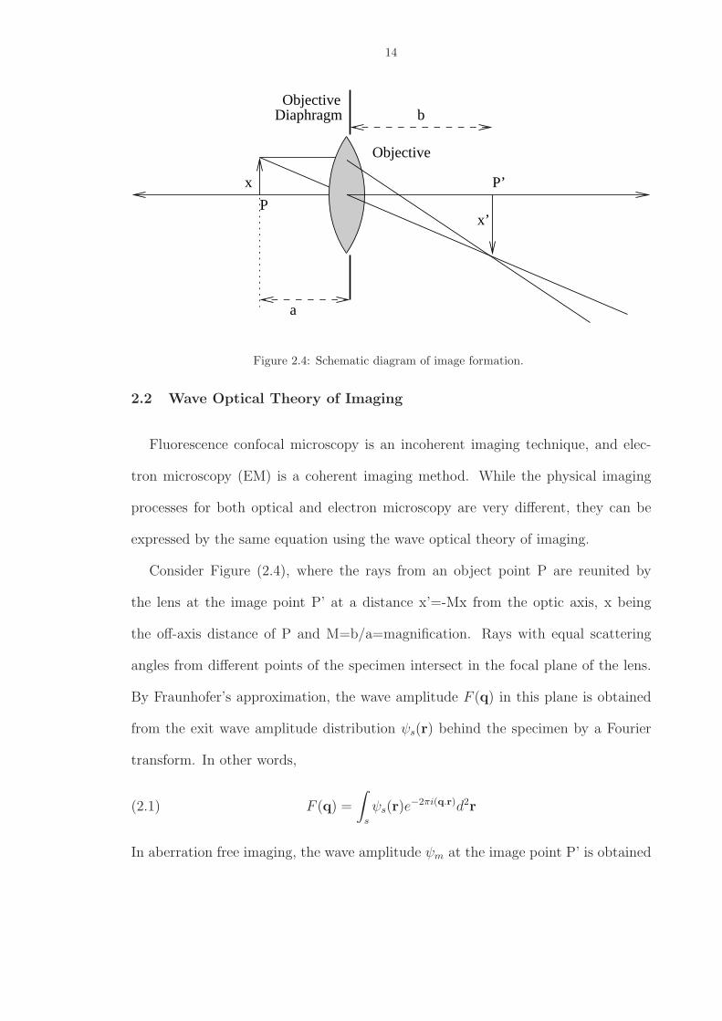
2.4 Schematic diagram of image formation. . . . . . . . . . . . . . . . . . . . . . . . . 14

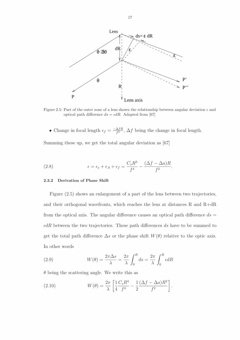
2.5 Part of the outer zone of a lens shown the relationship between angular deviationǫ and optical path difference ds = ǫdR. Adapted from [67] . . . . . . . . . . . . . . 17

4.1 Deconvolution test for noiseless data. Deconvolution of Elaine image . . . . . . . . 55

4.2 Deconvolution test for noiseless data. Deconvolution of Mandrill image . . . . . . . 56

4.3 A 201×201 image (a) blurred with a 35X35 Gaussian. (b) The resultant imageis shown in (c). The resulting reconstruction (d) was obtained after 17 rows andcolumns were discarded from the sides of the image. . . . . . . . . . . . . . . . . . 57

4.4 Performance of the deconvolution algorithm when only partial information is present.(a) is the original eye image that has been blurred by (b), a 7X7 Gaussian PSF.The reconstruction is shown in (c) showing little improvement. The plot in (d)shows the relation of Mean Square Error of the reconstruction with respect to theamount of pixels chopped from the edges before deconvolution was performed. . . 59

4.5 Comparision of MSE of TLS, LAP and STLN for Fourier Decomposition method. . 61

4.6 (a) is a section of the original image which has been blurred as shown in (b). (c)is the TLS reconstruction. Significant improvement is observed in (d) which is theSTLN reconstruction. . . . . . . . . . . . . . . . . . . . . . . . . . . . . . . . . . . 62

4.7 (a) L-curve obtained during the deconvolution of a 10X10 image with a 3X3 PSF.Figures (b)-(d) show the MSEs obtained using the Fourier decomposition and directmethods when deconvolution was performed on 4 × 4, 8 × 8 and 14 × 14 imagesconvolved with a 3 × 3 PSF respectively. . . . . . . . . . . . . . . . . . . . . . . . 64

5.1 30×30×30 bead image convolved with 3×3×3 PSF . . . . . . . . . . . . . . . . . . 79

5.2 Deblurred image . . . . . . . . . . . . . . . . . . . . . . . . . . . . . . . . . . . . . 79

vii

5.3 30×30×30 bead image convolved with 5×5×5 PSF with sides clipped off. . . . . . 80

5.4 Deblurred image. Note that the image is still a little blurry. . . . . . . . . . . . . . 80

5.5 MSE v/s SNR Comparisons of deconvolution of 3×3×3,5×5×5 and 7×7×7 imageswith 3×3 PSF . . . . . . . . . . . . . . . . . . . . . . . . . . . . . . . . . . . . . . . 81

5.6 MSE v/s SNR of STLN and Least Squares for a 9×9×9 image with a 3×3×3 PSF 81

5.7 MSE v/s SNR comparisions for our algorithm with Lucy-Richardson . Image:7×7,PSF 3×3 . . . . . . . . . . . . . . . . . . . . . . . . . . . . . . . . . . . . . . . . . . 82

5.8 Solution time v/s SNR comparison for our algorithm with Lucy-Richardson. Timeaxis is in seconds. Image 7×7, PSF 3×3 . . . . . . . . . . . . . . . . . . . . . . . . 82

6.1 Magnitude response of φ(n1, n2) = φ1(n1, n2) ∗ ∗φ2(n1, n2) . . . . . . . . . . . . . . 92

6.2 Sample QUILL model representation of an astronomical image. . . . . . . . . . . . 93

6.3 Sample QUILL model representation of a natural image. . . . . . . . . . . . . . . . 94

6.4 Sample QUILL model representation of a optical microscope image. . . . . . . . . . 94

6.5 Deconvolution of an image that was not constructed from the QUILL model. . . . 103

6.6 Deconvolution of an image that was convolved with a bandpass PSF. . . . . . . . . 104

6.7 Blind deconvolution of an image obtained from an optical microscope. . . . . . . . 105

6.8 Blind deconvolution of an image shot from a 3 Megapixel camera. . . . . . . . . . . 107

7.1 A representative CTF power spectrum estimated from carbon film backed cryo-EM data in (a) linear contrast and (b) logarithmic contrast stretch where the Thonrings are clearer. The elliptical shape is a result of astigmatism. . . . . . . . . . . 111

7.2 Examples of averaged CTF power spectra in logarithmic scale, obtained after sam-pling at 50 random points in the micrograph. Figure 7.2(a) is a representativeCTF obtained from a negative stained image. Due to the high SNR, Thon ringsare clearly visibile. Figure 7.2(b) is the CTF power spectrum obtained from acryo sample with carbon support film. Despite a lower SNR the first three Thonrings are still visible. Figure 7.2(c) depicts a CTF power spectrum obtained froma sample of bacteria flagella filament in ice. Due to the absence of carbon sup-port film the CTF is barely visible. The Fourier transform of the specimen is alsoobserved as lines in the power spectrum.[91] Figure 7.2(d) shows a representativepower spectrum from a cryo-EM tomograph. Due to the very low electron dose,the SNR of the CTF power spectrum is very low and the Thon rings are barely seen.116

7.3 Flowchart of defocus parameter estimation algorithm for planar and tilted samples. 120

viii

7.4 Measured defocus vs. Nominal defocus for carbon film EM data. The zero defocusoffset of the nominal defocus is 0.099 µm and is represented by the y-intercept ofthe least squares fit. The slope of the line is 1.005 and the correlation coefficient ofthe points with the least squares fit is 0.999 indicating that the quality of the fit isvery good. . . . . . . . . . . . . . . . . . . . . . . . . . . . . . . . . . . . . . . . . . 122

7.5 Comparision of defocus parameters obtained from 10 measurements our algorithmwith PLTCTFX [77] and ACE [52]. The graphs (from top to bottom) comparethe estimates obtained for ∆fmean, ∆fdiff and φA. The standard deviation of ourestimates are represented by the error bars. . . . . . . . . . . . . . . . . . . . . . . 124

7.6 Comparision of defocus parameters obtained from 10 measurements on 10 bacterialflagella filament samples embedded in ice with those of carbon film samples fromthe same micrograph. The mean defocus estimates in ice samples are in excellentagreement with the corresponding carbon film estimates (within 1200A). The astig-matism estimates are not reliable or consistent as indicated by the large differenceswith the carbon film estimates and by the high standard deviation of the ∆fdiff

estimates in ice. . . . . . . . . . . . . . . . . . . . . . . . . . . . . . . . . . . . . . . 126

7.7 Plot of theoretical and estimated offsets vs. distance from the rotation axis for57 negatively stained image samples tilted to 60◦. The solid line indicates thetheoretical defocus while the points indicate the average defocus estimate obtainedfor stripes parallel to the rotation axis. The error bars represent the standarddeviation of the estimates. The correlation coefficient between the theoretical andthe estimated defocus is 0.952 indicating a high degree of agreement. The smallerror bars indicate that the estimates are stable across the entire dataset. Theslope of the least squares fit through the average defocus estimates is tan(63.14◦)which is close to the theoretical value of tan(60◦). . . . . . . . . . . . . . . . . . . 128

7.8 Estimated mean defocus at rotation axis versus nominal mean defocus for Cryo-EM tilted series data. The specimen was rotated to 45◦. The CTF parameterswere determined for the projection of the specimen at the rotation axis at differentnominal defocii. The x-intercept of the plot is -0.156 µm which is the estimateof the absolute error in the nominal defocus value obtained from the microscopesetting. The slope of the line is 1.045 and the correlation coefficient between thepoints and the least squares fit is 0.997 indicating that the quality of the fit is good.129

7.9 Plots of ∆fo (mean defocus at rotation axis) and θtilt(tilt angle) versus slice numberfor a stack of tomographic cryo-EM data. The change in ∆fo with tilt angle is dueto eucentricity and specimen thickness. The tilt angle estimate agrees closely withthe nominal tilt indicating that the tilt angle was estimated correctly. The leastsquares fit over the tilt angle estimates (LS fit) closely follows the nominal tilt angleover the tilt series. . . . . . . . . . . . . . . . . . . . . . . . . . . . . . . . . . . . . 130

8.1 Flowchart of deconvolution process. . . . . . . . . . . . . . . . . . . . . . . . . . . 141

ix

8.2 Comparison of phase residual errors using edge preserving deconvolution with othermethods. The dashed line indicates the threshold above which noise is consideredto dominate the signal. The edge-preserving algorithm shows the least overallphase residual error among all the algorithms. Wiener filtering and phase flippingproduce comparable results. While both phase flipping with amplitude correctionand the quadratic gradient algorithm produce lower phase errors than phase flippingat the lower resolutions, their performance deteriorates at higher resolutions. Allalgorithms perform better than unregularized least squares at all resolutions belowthe noise threshold. . . . . . . . . . . . . . . . . . . . . . . . . . . . . . . . . . . . 143

8.3 A comparison of the cross sections of the 10 A 3D reconstruction of R-type bacteriaflagella filament. The top row figure denoted by M is the cross-section of the atomicmodel. It shows two well separated α helices in the core region indicated by theboxed regions marked by α1 and α2. The other top row figures denoted by P andE are obtained after phase flipping with amplitude correction [56] and after edgepreserving deconvolution respectively. The columns α1 and α2 highlight the α1 andα2 regions in the reference, phase flipped and edge preserved reconstructions. Fromthe figures, the α1 helices appear better separated in the edge preserving decon-volution reconstruction as compared to that obtained from the phase flipped andamplitude corrected version. Further, α2 helices of edge preserved reconstructionare more evident than the phase flipped image where they appear disk-like in shape.144

A.1 Defocus determination for a point U(x1, y1, z1) for a tilted image. O is the originof the coordinates. r′ is the rotation axis which is rotated θrot with respect tothe y-axis. p(x1, y1, θrot) is the distance of the projection of U(x1, y1, z1) from therotation axis on the zero tilt plane. . . . . . . . . . . . . . . . . . . . . . . . . . . 157

x

LIST OF TABLES

Table

4.1 Comparison of MSE of TLS, LAP and STLN for Direct Method . . . . . . . . . . . 61

xi

CHAPTER I

Introduction

For the past three decades, optical and electron microscopy (EM) have been the

tools of choice for viewing cellular and sub-cellular biological structures. One of

the key challenges in both of these imaging techniques is in viewing the specimen

of interest at the highest resolution and contrast. While increasing the laser beam

excitation in fluorescence microscopy or electron beam intensity in the case of EM

increases both contrast and resolution, it is not possible to do so indiscriminately.

High fluorescence excitation from a laser beam can cause photobleaching and per-

manently damage the specimen. Similarly, high electron beam radiation damages

delicate specimen. Thus, the challenge is to develop methods that preserve the spec-

imen while allowing them to be imaged at the desired resolution.

In all imaging systems, two factors ultimately limit the resolution of the image:

noise; and the the non-ideal response of the imaging system. Deconvolution refers to

a class of computational methods that aim to improve the contrast and resolution

of recorded images by reducing the effect of both of these factors. This approach to

resolution and contrast enhancement is attractive for two key reasons. First, it is

inexpensive, requiring little capital expenditure. Second, it is easy to deploy. A new

algorithm can be developed and deployed within weeks. Due to these advantages,

1

2

deconvolution has been an area of intense research in the fields of astronomy, biology,

geology, mathematics and engineering, and numerous deconvolution algorithms have

been developed over the past thirty years. For an overview, the reader is referred to

[76, 55, 4] .

Several technological improvements have revolutionized both optical and electron

microscopy in recent years. Optical microscopes have become very fast with some

of them able to image almost real time in 3-D at tens of frames per second. Elec-

tron microscopes have become less noisy and techniques have been developed to

analyze large molecules at atomic resolution. At the same time, improvements in

CCD technology have enabled images to be captured and stored digitally at high res-

olutions. Images captured with these microscopes after a successful deconvolution

would potentially enable imaging at unprecedented spatial and temporal resolution.

Unfortunately, conventional deconvolution algorithms are slow and are not suitable

for high throughput applications. Further, deconvolution algorithms for electron mi-

croscopy which are suitable for low-resolution images, are not very effective with high

resolution images.

In this thesis, we aim to address these problems by developing and exploring de-

convolution algorithms that are fast and easy to deploy. We show through simulations

and experiments on experimental data that our algorithms are able to deconvolve

images successfully, often better than conventional techniques.

1.1 Problem Overview

Conventional deconvolution algorithms are slow because they are iterative, re-

quiring many iterations to give a good result. Most of these algorithms require

measurement of the system response, also known as the transfer function, a time-

3

consuming and often difficult task. This makes them unsuitable for use in high

throughput applications where images have to be deconvolved quickly. Hence, there

is a need for non-iterative algorithms that can preferably deconvolve without the

transfer function information.

In EM, deconvolution is even more difficult, due to the very high noise levels of

these images. Many conventional algorithms overcome this by making unrealistic

assumptions which ultimately limit their effectiveness. The problem is exacerbated

by the fact that few algorithms have been developed that can estimate the transfer

function accurately. Thus, a good transfer function estimation method, coupled with

an effective deconvolution algorithm, would be an effective solution to this problem.

1.2 Previous Work

1.2.1 Optical Microscopy

One of the first deconvolution algorithms to be applied to optical microscopy

was the Van Cittert algorithm [1]. While fast, this algorithm does not promise

convergence and requires a good initial guess to give good results. Since then, several

deconvolution algorithms have been developed that fall roughly into two categories:

linear methods; and statistically derived methods.

Linear methods such as linear least squares, constrained least squares and Wiener

filtering, while simple to implement and fast, are commonly used in the context of

fluorescence microscopy [55]. Unfortunately, most linear methods suffer from two

problems. First, they are not very effective in restoring all spatial frequencies of

interest. This is especially problematic for the deconvolution of wide-field optical

microscopy images due to the ‘missing cone” problem [81]. Second, they overblur

the recovered image.

Statistically derived maximum-likelihood (ML) and maximum a posteriori (MAP)

4

algorithms are more sophisticated, as they allow the imaging noise to be modeled and

accounted for in the reconstruction. They may also allow some information about the

properties of the object to be included in the problem formulation[13, 54, 32, 33].

Unfortunately, while these methods often provide excellent reconstructions, their

iterative nature makes them very slow [55].

All the above methods require the estimation of the transfer function, also known

as the Point Spread Function (PSF) of the microscope, which is a measure of the

fidelity with which information is transferred from the input to the output of the

instrument. Although the form of the PSF is analytically well known, measuring it

accurately can be difficult and time consuming [55, 30]. Two potential classes of al-

gorithms attempt to solve this problem. The first, myopic deconvolution algorithms,

account for errors in the measured PSF and are partially able to overcome inac-

curacies in its measurement [31, 59]. The second, blind deconvolution algorithms,

attempt to deconvolve the image without any PSF information. This is a signif-

icantly more difficult problem than the other methodologies, and as a result it is

relatively unexplored. Further, both myopic and blind algorithms are slow [30].

1.2.2 Electron Microscopy

Deconvolution of EM images is more difficult than the optical case, for two reasons.

First, the images here are very noisy. In the case of cryogenic images, signal to noise

ratios (SNR) of 0 dB are quite common. Second, due to the low SNR, estimation

of the transfer function is very difficult. Without a good transfer function estimate,

most deconvolution algorithms will not give good object estimates.

Most algorithms developed in the field use Wiener filtering and its variants [49, 56,

14, 19, 6]. As in optical microscopy, these algorithms overblur the recovered images.

Another common approach is to use “phase-flipping” algorithms [56, 80]. While

5

simple to implement, these algorithms only correct for the phase distortions induced

by the transfer function. Moreover, many of these algorithms assume unrealistically

that astigmatism is absent in the system.

1.3 Contributions of this Thesis

In this thesis we develop and test four new algorithms. They are as follows:

• The first algorithm is a blind deconvolution algorithm that assumes that the PSF

is even, a reasonable assumption for many optical applications. This assumption

allows us to decompose the 2-D and 3-D blind deconvolution problem into many

small 1-D problems, which in turn speeds up the algorithm significantly. We

demonstrate that due to its speed, it become tractable to deconvolve large

images in a matter of minutes.

• The second algorithm is also a blind deconvolution technique that assumes that

the object can be represented by the a “QUILL” (Quincunx Upsampled Linearly

Interpolated) image model. This assumption allows us to break up the problem

into a four-blur problem, which can be solved quickly using well-established

results in multichannel blind deconvolution. This algorithm is well-suited to

large oversampled images at relatively high SNRs. These images are common

in fluorescence microscopy.

• The third algorithm is a transfer function estimation algorithm for cryo-EM

(cryo-EM) images. While several algorithms of the same class have been devel-

oped, this algorithm is unique for several reasons. First, this algorithm performs

the estimation in two dimensions, unlike most other algorithms that radially av-

erage the transfer function to increase the SNR of the transfer function image.

This is significant because radial averaging assumes astigmatism is absent in the

6

system, an assumption that is not true in most cases. Second, this algorithm

is the only algorithm that can estimate transfer functions for tilted images.

Third, this is one of two algorithms that has been developed with a Graphic

User Interface (GUI) and built on an Open Source Numerical Python platform.

This is significant because including the GUI makes the program easy to use for

biologists who do not have programming experience.

• The final algorithm deconvolves EM images using an edge-preserving regularizer.

We demonstrate that the algorithm reduces noise, while at the same time it

preserves high-frequency object information such as edges better than other

state of the art algorithms used in EM.

1.4 Organization of this Thesis

In Chapter II, we introduce the physics of image formation for both fluorescence

and electron microscopes. In Chapter III we develop the mathematical framework

of deconvolution and discuss conventional deconvolution techniques. In Chapters

IV-VI, blind deconvolution algorithms are introduced that are suitable for 2-D and

3-D fluorescence and optical microscopy. In Chapter VII, we present an automatic

transfer function determination algorithm for electron microscopy. In Chapter VIII,

we introduce an edge-preserving deconvolution algorithm and apply it to EM images.

Finally in Chapter IX, we present our conclusions and directions for future work.

CHAPTER II

Principles of confocal and electron microscopy

Biomedical imaging has made significant advances in recent decades. While it was

advances in physics that primarily led to new imaging modalities such as Magnetic

Resonance Imaging (MRI) and PET (Positron Emission Tomography) among others,

it was the digital revolution that extended the resolution of both new and time-

honored imaging techniques such as light microscopy.

Computational resolution extension algorithms for digital images, also known as

deconvolution algorithms, we first pioneered by astronomers in the early seventies [48,

68]. Unfortunately, CCD technology at this time was not at a point at which it could

be used for biological imaging applications. This precluded the use of computational

methods. It was only by the late eighties that the first deconvolution algorithms

for optical microscopy appeared. The algorithms of Jansson Van Cittert [41] and

others were adapted from well-established algorithms in astronomy and statistics.

With growing computational power, starting in the nineties, deconvolution has now

become an integral part of light and fluorescence microscopy [55].

The use of deconvolution for electron microscopy (EM) images has not been ex-

plored very much. This is due to two reasons: (1) Digital image capture and storage

is a relatively new technology in the EM area; (2) Until recently, EM images have

7

8

been very noisy. Conventional deconvolution algorithms would not have improved

the image quality very much. However, recent advances in EM hardware have made

these issues a thing of the past.

2.1 Introduction

2.1.1 The Confocal Microscope

Figure (2.1) shows a schematic diagram of a Laser Scanning Confocal Microscope

(LSCM),a commonly used microscope for fluorescence imaging. In LSCM, a laser

light beam is turned to a scanning beam and focused to a small spot by an objective

lens onto a fluorescent specimen. The fluorescent molecules in the illuminated object

are excited by incident light wavelength λex. The excited molecules emit light of

wavelength λem. The difference δλ = λem − λex > 0 between emitted and excitation

wavelength is called the Stokes shift of the fluorescent molecule.

The mixture of reflected light and emitted fluorescent light is captured by the

same objective, and after conversion into a static beam by the x-y scanner device,

it is focused onto a photo detector (photomultiplier) via a dichroic mirror (beam

splitter). The reflected light is deviated by the dichroic mirror, while the emitted

fluorescent light passes through in the direction of the photomultiplier. A confocal

aperture (pinhole) is placed in front of the photo detector, so that the fluorescent

light from points on the specimen that are not within the focal plane are largely

obstructed by the pinhole. In this way, out-of-focus information (both above and

below the focal plane) is greatly reduced. A lateral scan of the sample yields a 2-D

image. A lateral and axial scan yields a 3-D image.

9

collector

focal plane

illumination aperture

laser source

dichroic mirror

objective lens

sample

detectorPMT

lens

Figure 2.1: Schematic diagram of a laser scanning confocal microscope (LSCM)

2.1.2 The Transmission Electron Microscope

The principle behind the Transmission Electron Microscope (TEM) is similar to

that of the compound microscope in optics. As seen in Figure 2.2, a thermionic,

Schottky or field emission electron gun emits electrons. A condenser lens system

between the specimen and the electron gun ensures that the electron energy is op-

timally transferred to the specimen. After irradiating the specimen, the electrons

contain both phase and amplitude information about the sample. The emergent

electrons are then projected onto a photographic plate or a CCD array for recording

using a three-lens system.

In light microscopy, two stages of magnification is the norm, as the resolution of

the image is limited by the wavelength of light and the required magnification can

be obtained by using a two-lens system. In the electron microscope, however, the

10

Condenser 2

Condenser 1

Intermediate Lens

Projector Lens

Image

Objective

Selector Diaphragm

Electron gun

Objective Diaphragm

Figure 2.2: Schematic ray path for a transmisson Electron Microscope (TEM). Adapted from [67].

11

resolution is only limited by the spherical aberration of the lens, and not by the

wavelength of the electrons. Hence, three stages of magnification are needed to bring

the high magnifications necessary to bring the resolving power of the instrument up

to the resolving power of the eye.

The objective lens is a strong lens of short focal length that forms the primary

image of the specimen. This image is the object for the intermediate lens that is a

relatively weak lens of adjustable focal length. The image formed by the interme-

diate lens is then the object for the projector lens that performs the final stage of

magnification.

Electron microscopy is a coherent imaging method where the emergent electron

beam has both phase and amplitude information. Although the mathematical anal-

ysis of coherent imaging is different from incoherent imaging, we shall show that for

typical imaging conditions of biological samples the EM imaging equation is very

similar to the incoherent imaging equation.

2.1.3 Image Formation Processes in EM: A Qualitative Description

In EM, four physical processes, absorption, scattering, interference and diffraction

contribute to image formation. Absorption gives rise to amplitude contrast, interfer-

ence gives rise to phase effects, diffraction leads to formation of haloes and fringes

and scattering results in the formation of phase contrast. Diffraction is not discussed

in detail, as it is not an important process in EM image formation.

Scattering

Fast electrons passing through a specimen can interact either with the specimen

nucleii or with the electron cloud surrounding the nucleus. Due to the large mass

difference betweent the nucleus and electron, a fast electron passing close to the

12

nucleus is deflected by a large angle, suffering almost no energy loss. On the other

hand, a fast electron interacting with the slow electron orbiting the nucleus shares its

velocity with the slow electron, due to the law of conservation of angular momentum,

thereby suffering a change of direction and energy. Interactions of the first type are

known as elastic scatter, while the latter type of interactions are known as inelastic

scatter.

Scattering is the most important of all image formation processes in the electron

microscope, since it is the interference between the scattered and the unscattered

wave that leads to the development of a phase contrast.

Absorption

Absorption results in the formation of contrast based on mass-density. High

mass-density areas in the image plane appear dark, due to high local absorption

of electrons and low mass density areas. That is, electron-transparent areas appear

brighter, due to low absorption of electrons. Absorption is not an important factor for

thin biological specimens, as an electron has to encounter a whole series of inelastic

collisions for absorption.

Interference

For thin samples, which are typical in biological EM imaging, interference is an

important image formation process. Interference effects arise due to the following

two causes:

• Spherical Abberration: The objective lens of the electron microscope has an

uncorrectable spherical aberration. As a result, the path length of the elec-

tron beam passing through the periphery of the lens is longer than that of the

beam passing through the center. Thus rays from the same point can interfere,

13

Focus OverFocus

Imag

e co

ntra

st

UnderFocus

Figure 2.3: Variation of image contrast with objective lens focus. Defocussing increases the contrastof the image at the expense of resolution.

resulting in differences in intensity in the image plane. This effect is only ob-

servable close to the absolute limit of the resolution of the lens, and leads to

fine image granularity. Interference due to spherical aberration determines the

microscope’s ultimate resolving power.

• Defocussing: “Defocus contrast” refers to increase in contrast on either side of

the point of true focus. It is due to the formation of the Fresnel fringes about

any parts of the specimen where there is a rapid change in mass thickness. The

fringes enhance the lines and points resulting in an image of better contrast.

Unfortunately, defocussing also lowers the highest resolution attainable, and

may cause artifacts that appear to be “resolved” especially in images of regular

structures.

For biological samples, poor amplitude contrast necessitates artificial contrast en-

hancement by defocusing. However, due to the resolution-contrast tradeoff, the ap-

propriate defocus must be chosen carefully. Figure 2.3 shows the variation of contrast

with the defocus.

14

Diaphragm

Objective

b

a

P’

P

x

x’

Objective

Figure 2.4: Schematic diagram of image formation.

2.2 Wave Optical Theory of Imaging

Fluorescence confocal microscopy is an incoherent imaging technique, and elec-

tron microscopy (EM) is a coherent imaging method. While the physical imaging

processes for both optical and electron microscopy are very different, they can be

expressed by the same equation using the wave optical theory of imaging.

Consider Figure (2.4), where the rays from an object point P are reunited by

the lens at the image point P’ at a distance x’=-Mx from the optic axis, x being

the off-axis distance of P and M=b/a=magnification. Rays with equal scattering

angles from different points of the specimen intersect in the focal plane of the lens.

By Fraunhofer’s approximation, the wave amplitude F (q) in this plane is obtained

from the exit wave amplitude distribution ψs(r) behind the specimen by a Fourier

transform. In other words,

(2.1) F (q) =

∫

s

ψs(r)e−2πi(q.r)d2r

In aberration free imaging, the wave amplitude ψm at the image point P’ is obtained

15

by integrating over all elements of area d2q of the focal plane

(2.2) ψm(r) =1

M

∫ ∫F (q)e2πiq.rd2q =

1

Mψs(r)

In other words, ψm(r) is the inverse Fourier transform of F (q). In aberration free

imaging there will be no further phase shift. In practice, a maximum scattering

angle θmax = α0 (objective aperture) corresponding to a maximum spatial frequency

qmax is used. The limitation on spatial frequencies by an objective diaphragm can

be expressed by a multiplicative masking M(q) = 1 for q = |q| < qmax and M(q) = 0

otherwise in the normal bright field mode.

If wave abberation is only a function of q, the action of this contribution can be

represented as a multiplication of amplitudes in the focal plane by a phase factor

e−iW (q). We rewrite the wave amplitude at P’ as

(2.3) ψm(r) =1

M

∫ ∫F (q)

[e−iW (q)M(q)

]e2πiq.rd2q =

1

Mψs(r)

We set H(q) =[e−iW (q)M(q)

]. H(q) is known as the pupil function. Setting h(r) =

F−1(H(q)) , (the inverse Fourier transform of the pupil function), we can write

(2.4) ψm(r′) =1

Mψs(r) ⊗ h(r)

where ⊗ is the convolution operator. h(r) is known as the point spread function

(PSF).

(2.4) is a general form of image formation equation. In the case of incoherent

image formation, such as fluorescence microscopy, we are only concerned about the

intensity of ψm(r′). Hence the distribution can be written as a scalar. The ideal

intensity image for a confocal microscope can be expressed as [51]

(2.5) i(r) = h(r) ⊗ o(r)

16

where i(r) is the image, o(r is the object. Using scalar ordinate variables, the 2-D

PSF is given by [51]

(2.6) h(r) = F−1[|H1(q, φ)|2|H2(q, φ)|2

].

Here H1(q, φ) is the Fourier transform of the point spread function of the objective

lens, H2(q, φ) is the Fourier transform of the point spread function of the collector

lens, q is the spatial frequency and φ is the angle ordinate in the frequency plane.

Applying the Fourier transform, (2.5) can be expressed a multiplicative process

in the frequency plane as

(2.7) I(q, φ) = H(q, φ)O(q, φ)

where q, φ are the radial ordinates in the spatial frequency plane.

In the case of EM the imaging equation is not as simple due to the coherence in

the image formation process. Fortunately, for thin biological specimen, the imaging

equation can be approximated to a form identical to (2.7). We shall derive the EM

imaging equation in the next section.

2.3 Derivation of EM Imaging Equation

2.3.1 Angular Deviation of Wavefront in an Electron Lens

When a wavefront passes through an electron lens, it is subject to an angular

deviation causing a phase shift in the wavefront. The angular deviation has three

causes:

• Spherical abberation: ǫs = CsR3

f4 , Cs being the spherical aberration coefficient, f

being the focal length and R being the distance of the lens from the optic axis.

• Change in specimen position ǫa = ∆aRf2 , a being the distance of the object from

the lens and ∆a being the change in specimen position.

17

ε dRds=Lens

θ + δθ

θR

dR εε

P’

P’’

PLens axis

Figure 2.5: Part of the outer zone of a lens shown the relationship between angular deviation ǫ andoptical path difference ds = ǫdR. Adapted from [67]

• Change in focal length ǫf = −∆fRf2 , ∆f being the change in focal length.

Summing these up, we get the total angular deviation as [67]

(2.8) ǫ = ǫs + ǫA + ǫf =CsR

3

f 4− (∆f − ∆a)R

f 2.

2.3.2 Derivation of Phase Shift

Figure (2.5) shows an enlargement of a part of the lens between two trajectories,

and their orthogonal wavefronts, which reaches the lens at distances R and R+dR

from the optical axis. The angular difference causes an optical path difference ds =

ǫdR between the two trajectories. These path differences ds have to be summed to

get the total path difference ∆s or the phase shift W (θ) relative to the optic axis.

In other words

(2.9) W (θ) =2π∆s

λ=

2π

λ

∫ R

0

ds =2π

λ

∫ R

0

ǫdR

θ being the scattering angle. We write this as

(2.10) W (θ) =2π

λ

[1

4

CsR4

f 4− 1

2

(∆f − ∆a)R2

f 2

].

18

We approximate R/f ≈ θ (θ being the deflection angle) and defocussing ∆z =

∆f − ∆a. Substituting we get the Scherzer formula [67]

(2.11) W (θ) =π

2λ(Csθ

4 − 2∆zθ2)

Conventionally, when ∆z < 0 it is called overfocussing, and when ∆z > 0 it is called

underfocussing. Introducing the spatial frequency q = θ/λ (its derivation comes from

wavefront theory) we get

(2.12) W (q) =π

2(Csλ

3q4 − 2∆zλq2)

Finally, we introduce an additional term for axial astigmatism

(2.13) WA = −π

2q2λ∆fdiff cos [2(φ − φa)]

where φ is the azimuthal angle, χ0 is the azimuthal angle for the direction of defocus,

∆fdiff is the amount of focus difference due to astigmatism. We approximate ∆z ≈

∆fmean. Hence, the total phase is now

(2.14) W (q) =π

2

[Csq

4λ3 − λq2(2∆fmean + ∆fdiff cos(2φ − 2φa))]

2.3.3 Weak Amplitude Weak Phase Approximation

By Fraunhoffer’s approximation, the exit wave amplitude after passing through a

specimen can be described by

(2.15) ψ = ψoas(r)eiϕs(r)e2πikz = ψse

2πikz

where r is the radius vector in the specimen plane from the origin on the optic axis,

as(r) is the local decrease of amplitude due to absorption, and ϕs(r) is the phase

shift caused by the specimen[67]. We normalize the amplitude ψo to unity. Next we

assume that the sample is thin, so that there is a very small amount of absorption.

19

Hence, we can assume as(r) = 1−ǫs(r) where ǫs(r) is small. Assuming that the phase

shift is also much less than one, the exponential term in (2.15) can be expressed as

(2.16) ψ(r) = 1 − ǫs(r) + iϕs(r) + . . .

With this approximation, the object is said to be weak-phase-weak-amplitude.[79]

In practice, specimens thinner than 10 nm and composed of low atomic number

elements such as a hydrogen, carbon, oxygen and nitrogen behave as weak phase

objects.

2.3.4 The Contrast Transfer Function

Hanzen and coworkers [26] developed the concept of the Contrast Transfer Func-

tion (CTF) for electron microscopy. This enabled the description of an objective lens

independent of any particular specimen structure.

In (2.3), consider an idealized point specimen that scatters light isotropically, so

that it is a source of spherical waves of amplitude f(θ), independent of the scattering

angle θ. By definition, the point spread function is obtained as the image of this

specimen. Introducing polar coordinates r′ and φ in the image plane and setting

magnification to 1, the scalar product becomes q · r = qr′ cos φ = θr′ cos φ/λ; we

have d2q = θdθ/λ2 and F (q) = λf(θ). We then get

(2.17) ψm(r′) =1

0+

i

λ

∫ α0

0

∫ 2π

0

f(θ)e−iW (θ)e2πiλ

θr′ cos φθdθ

where we use 1 for brightfield mode and 0 for dark field mode. The factor i indicates

a phase shift of π/2 between primary and scattered waves. The difference between

bright and dark field modes is that in the former, the primary incident wave (nor-

malized to 1) contributes to the image amplitude, whereas in the dark field mode it

20

is absorbed by a central beam stop or a diaphragm. The factor i indicates a phase

shift of 90◦ between incident and scattered waves.

Applying the weak amplitude weak phase approximation to this point specimen,

using (2.16) for a single spatial frequency q, we can represent the point object’s local

amplitude modulation and phase shift by ǫs(r) = ǫs(2πqx) and ϕs(r) = ϕq(2πqx)

giving

(2.18) ψs(x) = 1 − ǫq cos(2πqx) + iϕq cos(2πqx) + . . .

Using (2.17), the image intensity becomes

(2.19) I(x′) = |ψm(x′)|2

(2.20) I(x′) = 1 − D(q)ǫq cos(2πqx′) − B(q)ϕq cos(2πqx′)

The CTF is defined as the Fourier transform of the point spread function. Hence,

D(q) = 2 cos W (q) is the CTF of the amplitude structure of the specimen and, using

(2.12),

(2.21) B(q) = −2 sin W (q) = −2 sin[π

2(Csλ

3q4 − 2∆zλq2)]

is the CTF of the phase structure.The sign of B(q) is chosen so that B(q) > 0 for

postive contrast. Using (2.14) the phase CTF is given by

(2.22) B(q) = 2 sin(π

2

[Csq

4λ3 − λq2(2∆f + ∆fdiff cos(2φ − 2φa))])

Tani et al [77] use a CTF formula that accounts for both phase and amplitude

contrast. To derive this form, consider (2.20). Setting ∆φ = cos−1( ϕq√ϕ2

q+ǫ2q) we can

21

express the intensity as

(2.23) I(x′) = 1 + 2 cos(2πqx′) sin(W (q) − ∆φ)

Hence the CTF is expressed as

(2.24) CTF (q, φ) = sin(π

2

[Csq

4λ3 − λq2(2∆f + ∆fdiff cos(2φ − 2φa))]− ∆φ)

2.3.5 EM Imaging Equation

Using the theory of contrast transfer, the ideal image formation process can be

described by

(2.25) I(q, φ) = CTF (q, φ)O(q, φ)

where I(q, φ) is the Fourier transform of the image and O(q, φ) is the Fourier trans-

form of the object.

In this chapter, we have assumed ideal imaging conditions. Noise from sources

such photo-detection and photon-counting have not been considered. In the case of

EM, we have not included the background signal due to inelastic scatter and the

envelope function due to incoherence of the electron beam, stage drift etc [73],[52].

In the subsequent chapters, these issues will be taken into account.

CHAPTER III

Principles and approaches for the deconvolution problem

For incoherent imaging modalities such as optical and fluorescence microscopy

and biological electron microscopy, the image formation process can be modeled

as a convolution of the object signal with a transfer function. As a result, the

image is a distorted version of the object itself, which ultimately limits the resolution

available from the imaging instrument. Deconvolution aims to correct the image

for distortions due to the transfer function, system noise and other non-idealities of

the imaging process, thereby improving the imaging resolution.

In this chapter, we briefly study the general image formation process. Next,

we briefly describe some of the common deconvolution algorithms that have been

developed from linear system theory, and also from a statistical perspective. Finally,

we study the Automatic Image Deconvolution Algorithm (AIDA) that forms the

basis of Chapter VIII.

3.1 Basic Equation

We assume throughout that the object is spatially bandlimited so that the prob-

lem can be spatially sampled. Then in many 2-D imaging applications the image

formation process can be modeled as [44, 72]

22

23

(3.1) y(n1, n2) = h(n1, n2) ⊗ o(n1, n2) + n(n1, n2)

where

(n1, n2) are the discrete pixel coordinates of the image frame;y(n1, n2) is the blurred image (output from device or process);o(n1, n2) is the true image;h(n1, n2) is the transfer function (TF)

also known as Point Spread Function (PSF)n(n1, n2) is additive noise, and;⊗ is the discrete 2-D linear convolution operator.

Taking the 2-D DSFT (Discrete Space Fourier Transform) yields

(3.2) Y (ω1, ω2) = O(ω1, ω2)H(ω1, ω2) + N(ω1, ω2)

The resulting image y is not an accurate visualization of the object o, since it is

a filtered version of o that has been distorted by noise. Deconvolution algorithms

attempt to correct the image for the effects of the transfer function, thereby providing

an image that better represents the object.

In the Fourier domain, we want to determine O(ω1, ω2) knowing Y (ω1, ω2) and

H(ω1, ω2). A naive approach would be a simple division of image Y by the transfer

function H, i.e.

(3.3) O(ω1, ω2) =Y (ω1, ω2)

H(ω1, ω2)= O(ω1, ω2) +

N(ω1, ω2)

H(ω1, ω2)

This method, called the Fourier quotient method [41] or inverse filtering [55]

gives very poor and unstable results, since the inverse filter 1H

is large at frequencies

for which H is very small (typically, high frequencies). This results in large noise

amplification, and thus a poor reconstruction. As a result, Fourier approaches adopt

some strategy to reduce noise amplification.

24

A variety of deconvolution algorithms have been developed, reflecting the differ-

ent ways of obtaining the best estimate of the true object. If one has good prior

knowledge of the PSF (which is often the case in microscopy), then simple modeling

of PSF with a set of variable parameters is used [41]. In many cases, only partial

information of the PSF is available, in which case myopic deconvolution methods are

used. Finally, in some cases, no information of the PSF may be available, in which

case blind deconvolution methods are used.

3.1.1 The Partial Data Problem

In applications such as remote sensing or microscopy, the unknown image often

does not have compact support (there is no compact region outside of which the

image is known to be zero). Rather, it is just part of a bigger image. In this case,

the blurred image that constitutes the data is actually smaller than the image to

be reconstructed. This is called the partial data problem [28]. The difficulty of

this problem is that it can be formulated as an under-determined system of linear

equations. We shall show in the coming sections how one of our algorithms is able

to overcome this issue.

3.1.2 The Case For Blind Deconvolution

Deconvolution is an ill-posed problem. This means that small errors in image or

PSF information will lead to large errors in object estimates. This problem has tra-

ditionally motivated statistical deconvolution methods in which some or all available

system information is incorporated in the algorithm in order to make the algorithm

more robust. Unfortunately, regardless of the application,obtaining an accurate PSF

is difficult [55, 41]. Even if a theoretical PSF model is used, it cannot account for

model imperfections. Moreover, in applications such as microscopy, obtaining the

25

PSF is often time consuming and difficult [55].

Blind deconvolution algorithms seek to estimate not only the original image but

also the PSF. In doing so, these methods hold promise for accurate determination of

the object. Until now, blind deconvolution algorithms were not very popular, as the

difficulty of the problem made computation times very high and often impractical.

However, as we shall show in Chapters IV, V and VI, in some cases, a linear algebraic

approach to this problem can give us excellent images, often better than non-blind

statistical methods.

3.1.3 A Brief Overview of Common Deconvolution Algorithms

Deconvolution algorithms generally fall under two categories: linear algorithms

that have been developed with a deterministic approach; and statistical algorithms

that use a probabalistic approach.

3.1.4 Linear Methods

Linear methods aim to find the optimal object estimate that minimize the noise

term in (3.1) using either a least squares or total least squares approach [35],[36],[47],[63].

Stated mathematically, we find o(n1, n2) such that

(3.4) o(n1, n2) = argmino(n1,n2)

‖n(n1, n2)‖2 = argmino(n1,n2)

‖y(n1, n2)− o(n1, n2)⊗ h(n1, n2)‖2

A direct minimization of equation (3.4) will produce unstable results due to the

ill-posed and ill-conditioned nature of the problem. The results can be made more

stable by using Tikhonov regularization. The regularized solution is expressed as

(3.5)

o(n1, n2) = argmino(n1,n2)

‖y(n1, n2) − o(n1, n2) ⊗ h(n1, n2)‖2 + λ‖f(n1, n2) ⊗ o(n1, n2)‖2

where f(n1, n2) is a penalty function applied to the data. This error criterion contains

two terms, the first representing the fidelity to the data, and the second representing

26

avoiding roughness in the restored image [41]. λ is the regularization parameter and

represents the trade off between data fidelity (variance) and image fidelity (bias).

Finding λ requires numerical techniques such as generalized cross validation [43];

there is vast literature on this topic which we will not review here. The solution to

(3.5) is easily expressed in the frequency domain as

(3.6) O(ω1, ω2) =H∗(ω1, ω2)Y (ω1, ω2)

|H(ω1, ω2)|2 + λ|F (ω1, ω2)|2

Generalizing this, we get the filtering [3] solution

(3.7) O(ω1, ω2) =W (ω1, ω2)Y (ω1, ω2)

H(ω1, ω2).

W (ω1, ω2) is typically a Gaussian, Hanning, Hamming or Blackman window [61].

Linear regularized methods are very attractive from a computational point of view

but also suffer from some drawbacks:

• The Wiener and Tikhonov restoration filters are both convolution filters. Their

linear nature makes them incapable of restoring frequencies for which the PSF

has zero response. In particular, the PSF of a 3-D widefield fluorescence micro-

scope has large regions in the frequency domain with zero response known as

the missing cone. These cannot be restored and leads to Gibbs oscillations.

• It is difficult to incorporate a priori information.

One can improve on least squares by using constrained least squares methods [35, 47],

which typically enforce non-negativity in the solution. The solution is no longer

obtained in a one-pass process, but instead it is obtained iteratively. A commonly

used method is the Tikhonov-Miller method, which uses conjugate gradients to solve

the problem. The Tikhonov-Miller method provides a theoretical bound on the error

in the reconstructed image[9]. The interested reader is referred to [81].

27

3.1.5 Statistical Methods

Statistical methods treat the deconvolution problem as one of estimating an un-

known object o(n1, n2) from noisy measurements y(n1, n2). This approach allows us

to use well known methods from estimation theory. While there are several different

statistical methods to solve this problem, the three approaches that are most com-

monly used are: maximum-likelihood (ML) estimation; Bayesian estimation; and

penalized likelihood estimation. Each of these is briefly discussed in the coming

sections. The interested reader is referred to [17, 29, 74, 68] for more details.

Maximum Likelihood Methods

Maximum likelihood (ML) methods aim to maximize the “agreement” between

the measurement (the image y) and the object o. Mathematically,

(3.8) o = argmaxo

log p(y|o)

For additive zero-mean white Gaussian noise, ML methods are identical to the de-

terministic methods discussed above, with no penalty functions. As a result, ML

methods often result in noisy solutions [17].

Bayesian Methods

Bayesian estimators provide a framework to incorporate information about the

object, thereby constraining the solution. This leads to more stable estimates in the

presence of noise. The object information is incorporated as a “prior”, denoted here

by p(o).

Bayesian estimation is most commonly used with the Maximum A Posteriori

(MAP) approach, where the solution is defined as

(3.9) o = argmaxo

p(o|y).

28

We need Bayes rule, which is

(3.10) p(o|y) =p(y|o)p(o)

p(y)

Applying the logarithm to both sides and ignoring p(y) as it is independent of o

gives,

(3.11) oMAP = argmaxo

[log p(y|o) + log p(o)]

If both the noise and the object are modelled by white Gaussian random fields,

MAP methods are identical to the deterministic methods discussed above, where

log p(o) plays the role of the penalty function. If the variance of p(o) is infinite, then

MAP reduces to ML.

A major drawback of Bayesian estimation is that it is difficult to design priors

that represent the true object accurately. This problem is overcome in the penalized

likelihood approach discussed next [17].

Penalized likelihood approach

The MAP estimator attempts to maximize two terms. The first term quantifies

the agreement of the distorted object with the measurement. The second term

quantifies the agreement with the prior expectation about the object. In contrast,

the penalized likelihood method attempts to minimize two terms; the first term

quantifies the disagreement of the distorted object and the measurement, and the

second term quantifies the disagreement of the estimate with the expected properties

of the object. Mathematically,

(3.12) oPL =

[argmin

o− log p(y|o) + λR(o)

]

Since the term log p(y|o) measures the fidelity of the estimate to the observed

data, it is known as the data fidelity term.

29

The term λR(o) is the penalty function that regularizes the estimate. The term

λ is known as the regularizing parameter [17] or hyperparameter [59].

While (3.11) and (3.12) look similar, they are philosophically very different. The

“prior” term in Bayesian estimation is a function of the object itself; it does not vary

with the measurement. In the penalized likelihood approach, we are only concerned

about the deviation of the estimate from a certain property of the object, allowing

us to change the penalty term depending on the measurement. With the penalized

likelihood approach, it is simpler to design and implement penalities incorporating a

priori object information than it is to do the same with statistical priors in the MAP

approach.

3.2 The Automatic Image Deconvolution Algorithm

The Automatic Image Deconvolution Algorithm (AIDA) is a myopic deconvolu-

tion algorithm devloped by Hom et al. [31]. The algorithm is based on the Myopic

Iterative STep preserving Restoration ALgorithm (MISTRAL) that was developed

for astronomy using a penalized likelihood approach [59]. Although the theoretical

development for both algorithms is very similar, AIDA different from MISTRAL in

a key way: the hyperparameter is estimated automatically in AIDA, while it has to

be determined by trial and error in MISTRAL. This makes AIDA automatic, easy

to use, and faster than MISTRAL.

In the rest of this section, we discuss the theory behind the AIDA algorithm.

We first discuss the choice of the noise model, data fidelity term, and penalizing

function. Next, we discuss the myopic scheme which allows for the joint estimation

of the transfer function and the object when the transfer function is not known very

well. Finally, we study the hyperparameter estimation scheme which enables AIDA

30

to be fully automatic.

3.2.1 AIDA Noise Model

In a typical digital imaging setup, we can make the following assumptions: (i) The

image formation process is linear and space invariant; (ii) signal-dependent Gaussian

and Poisson noise sources are present [70]; and (iii) the response of each CCD pixel

is independent of the others. This allows us to write the imaging equation as

(3.13) y(n1, n2) = o(n1, n2) ⊗ h(n1, n2) ◦ np(n1, n2) + nG(n1, n2)

where np(n1, n2) is a Poisson process with variance σ2P and nG(n1, n2) represents a

zero-mean Gaussian random field with variance σ2G. When images are not photon

limited, a good approximation to the above noise model is[59, 31].

(3.14) w(n1, n2) ∼ N(o, σ2w(n1, n2))

where

(3.15) σ2w(n1, n2) = σ2

G + σ2P (n1, n2)

The variance σ2G and the variance map σ2

P can be estimated from the image. Assum-

ing the image is background subtracted, one can estimate σ2G by fitting the histogram

of negative-valued pixels with the left half of a zero centered Gaussian.

(3.16) σ2G =

π

2

[< y(n1, n2) >((n1,n2);y(n1,n2)≤0)

]2

If the image does not have any negative pixels, as is often the case in microscopy,

a separate dark image is required to estimate σ2G. The Poisson contribution (variance

map) can be calculated as [31]

(3.17) σ2P (n1, n2) = max [y(n1, n2), 0]

31

This estimate is quite accurate for bright areas where the photon noise contri-

bution is much greater than the Gaussian noise. In dark regions this estimate is

unimportant, as the Gaussian noise dominates over the Poisson noise contribution.

3.2.2 Data Fidelity Term

We use a weighted maximum likelihood term to describe data fidelity:

(3.18) Jn(y|o) =1

2

∑

n1,n2

[y(n1, n2) − o(n1, n2) ⊗ h(n1, n2)]2

w(n1, n2)

where

(3.19) w(n1, n2) = σ2G + σ2

P (n1, n2)

w(n1, n2) acts as a weighting term. When w is large for a given (n1, n2), the data

at that point is considered less “reliable”, and its contribution to the cost function

Jn(y|o) is smaller.

3.2.3 Regularization Term

Most objects in microscopy are smooth or piecewise-smooth. (3.18) may be

quadratically regularized using a Gaussian prior. However, quadratic regulariza-

tion tends to oversmooth the image at the edges, as the Gaussian prior model is not

particularly well-suited to real world images [17].

AIDA solves this problem by using the edge-preserving regularizer proposed by

Brette and Idier [7, 31]. This regularizer is similar to the Huber functional in that

it is quadratic for small gradients and linear for large ones [17]. The quadratic

part ensures a good smoothing of the small gradients (often caused by noise), while

the linear portion prevents over-penalization of the large gradients to preserve the

edges (unlike quadratic regularization). The edge-preserving term is mathematically

32

described as [31]

Jo(o) = λo

∑

n1,n2

φ(γ(o, θn1,n2))(3.20)

φ(γ) = γ − ln(1 + γ)(3.21)

γ(o, θn1,n2) =

‖∇o(n1, n2)‖θn1,n2

(3.22)

where ||∇o(n1, n2)|| = [(∇xo(n1, n2))2 + (∇yo(n1, n2))

2]1

2 and ∇xo(n1, n2) and ∇yo(n1, n2)

are the object gradients along x and y respectively. The terms θn1,n2and λo are known

as the “hyperparameters” of the object prior [59].

The term φ(γ) characterizes the local texture of the object. It is called the clique

potential. When γ is small, (3.21) approximates to φ(γ) = γ−(γ−γ2/2+. . .) ≈ γ2/2;

for large γ , φ(γ) = γ.

The hyperparameter terms λo and θn1,n2control the amount of regularization. λo

controls the tradeoff between data fidelity and the edge preservation, while θn1,n2

determines when the regularization transitions from being quadratic to being linear.

3.2.4 Myopic Deconvolution

Until now we have assumed that the transfer function is known accurately and the

only unknown is the object. In many realistic cases, this is untrue. When the transfer

function is poorly known or not known at all, the problem becomes ill-conditioned

and ill-posed for the following two reasons: (1) The transfer function is bandlimited

by the imaging system; and (2) Noise is present beyond the bandwidth of the system.

Several approaches have been attempted to solve this problem. They generally

fall into two categories. In the first, deconvolution is attempted with the assumption

that the transfer function is unknown [29, 89]. This is known as blind deconvolution.

However, apart from a few specialized cases, blind deconvolution algorithms are not

very effective. Constraints such as positivity [44] of the object and transfer function

33

do aid in deconvolution, but even this scheme is not very effective for large PSFs.

The other class of approaches fall into the Myopic deconvolution category. Here,

the transfer function is known but is poorly characterized. AIDA and MISTRAL

use this approach where the principle is to constrain the transfer function softly at

all frequencies and then jointly estimate the transfer function and object in a MAP

framework. We modify (3.10) for the joint estimation as :

(3.23) p(o, h|y) =p(y|o, h)p(o)p(h)

p(y)

The joint estimates can be written as

(3.24) [o, h] = argmino,h

− log p(y|o, h) − log p(o) − log p(h)

The only new term in this scheme is the last one, which accounts for the partial

knowledge of the transfer function. We use the following Fourier domain constraint

(3.25) Jh(h) =λH

2

∑

ω1,ω2

|H(ωx, ωy) − H(ωx, ωy)|2v(ωx, ωy)

where λH controls the transfer function regularization relative to the data-fidelity

term of (3.12), H(ωx, ωy) is the Fourier transform transfer function estimate, H(ωx, ωy)

is the Fourier transform of the averaged PSF. v(ωx, ωy) is the sampling variance or

the power spectral density of the transfer function, and is defined as

(3.26) v(ωx, ωy) =<| H(ωw, ωy)−H(ωw, ωy) |>2=<| H(ωw, ωy) |>2 − | H(ωx, ωy) |2

v(ωx, ωy) serves as a spring constant that constrains each frequency component of

the transfer function to a mean value dervied from a set of transfer functions. Conan

et al. [12, 20] have shown that this constraint (also known as a harmonic Optical

Transfer Function (OTF) constraint [31]) performs much better in recovering the

true PSF than simple bandlimiting of the PSF.

34

3.2.5 Automatic Hyperparameter Estimation

The MISTRAL algorithm requires a manual selection of the hyperparameters

θn1,n2, λo for effective regularization. To deconvolve an image optimally, one has

to deconvolve the image for a variety of θn1,n2, λo sets from which “acceptable” re-

construction θn1,n2, λo sets are found. Usually, a plane of such acceptable solutions

are found, suggesting that when one hyperparameter is optimally defined the other

hyperparameter can be adjusted for optimally balancing the data-fidelity and edge

preserving terms [31].

Hom et al. [31] developed an automatic parameter estimation scheme based

on the assumption that the probability distribution of the pixels in an image can

be interpreted as a Gibbs distribution. If J(x) is the cost function and Z(x) =

∫xexp [−J(x)] dx is the partition function, then the probability distribution of the

pixels is modelled as being given by [5, 22]

(3.27) p(x) = exp [−J(x)] /Z(x)

With this assumption, we can define an image as optimally regularized when the

Gibbs free energy distribution of all the pixels of the data fidelity term − log p(y|o, h),

equals that of the edge-preserving object term − log p(o). Defining δ ≡ i− o⊗h and

ζ(n1, n2) as the combined Gibbs free distribution of all the pixels, we define

(3.28) ζn(n1, n2)δ ≡∫

δ

exp[−(δn1,n2

)2/2w(n1, n2)]dδ

ζo(n1, n2)‖∇o(n1,n2)‖ ≡∫

‖∇o(n1,n2)‖

exp

[−λo

(‖∇o(n1, n2)‖θ(n1, n2)

− ln

(1 +

‖∇o(n1, n2)‖θ(n1, n2)

))]d‖∇o(n1, n2)‖

(3.29)

35

Equating these integrals, we get

(3.30) ζn(n1, n2)δ = ζo(n1, n2)‖∇o(n1,n2)‖

√2πw(n1, n2) = θn1,n2

eλ

∫ ∞

1

e−λt/t−λdt(3.31)

= θn1,n2

(1

λo

+ 1

)(3.32)

where the approximation holds for λo ≤ 10. By equating these integrals on an

element-by-element basis, we are intrinsically assuming that the Gibbs distribution

of (3.27) can be represented as a product of sepearable functions. That is, we are

assuming that the pixels are independent and identically distributed (i.i.d.). This is

also known as the mean-field approximation. Solving for λo in (3.31) gives

(3.33) λo = (√

2πw(n1, n2)/θn1,n2− 1)−1

We can now set

(3.34) θn1,n2=

√w(n1, n2)/σG

Substituting θn1,n2in (3.33), we get a pixel-independent expression for λo.

(3.35) λo = (√

2πσG − 1)−1

This scheme was found to give good object estimates [31]. In cases where this

scheme over-regularized due to model mismatch, scaling the hyperparameter up or

down by no more than a factor of 10 was found to be sufficient.

The λH parameter from (3.25) also needs to be balanced. By the power conser-

vation relation of Parseval’s theorem we know∑N−1

r=0 |x(r)|2 = (1/Nd)∑N−1

k=0 |X(k)|2.

36

The λH term operates on a reciprocal space term. Hence, to heuristically balance

λH with respect to the other terms, we set

(3.36) λH = 1/Nd

Nd being the number of pixels in the image.

CHAPTER IV

2-D blind deconvolution of even point-spread functions from

compact support images

4.1 Introduction

4.1.1 Blind Deconvolution

The problem of reconstructing a 2-D image with compact support from its 2-

D convolution with an unknown blurring or point-spread function (PSF) arises in

several disciplines [44], including image restoration from an unknown blurring agent,

remote sensing through the atmosphere, and medical imaging. A good introductory

review of the history and applications of this problem is available[44].

In many applications in optics, acoustics and electro-magnetics, the point-spread

function may be assumed to be an even function of its spatial variables, due to

reciprocity. To see this, let u(xo) be the electromagnetic or acoustic field strength at

spatial position xo. The response u(yo) to an excitation or source s(xo) is u(yo) =

∫G(yo, xo)s(xo)dxo, where G(yo, xo) is the Green’s function. If the Green’s function

is translation-invariant, then G(yo, xo) = G(yo − xo). If reciprocity holds, then by

definition G(yo, xo) = G(xo, yo), and G(·) is an even function.

Since both the image and the point-spread function can be assumed to have

finite spatial extent (i.e., finite support), their Fourier transforms may be sampled

in wavenumber. Most images are approximately bandlimited to the extent that they

37

38

may also be sampled spatially as well. This leads to the discrete version of this

problem, in which a discrete-time image known to have finite spatial extent is to

be reconstructed from its convolution with an also-unknown point-spread function

(PSF). This precludes methods based on oversampling of continuous images.

4.1.2 Previous Work

A common approach for blind deconvolution problems is to use an iterative trans-

form algorithm [44], which alternate between the spatial and wavenumber domains.

However, these algorithms often stagnate, failing to converge to a solution[18, 83].

Other approaches require the computationally expensive and extremely unstable nu-

merical operation of tracking zero sheets of algebraic functions, or statistical estima-

tion algorithms that also may not converge. Another iterative approach (NAS-RIF)

is guaranteed to converge, but assumes the PSF has an inverse PSF of small size.

We will not attempt to list all approaches here.

The problem addressed in this paper should be distinguished from the problem

of multichannel blind deconvolution, addressed in many recent papers. In the latter

problem, a single unknown signal or image is filtered with several unknown blurring

functions, resulting in several known outputs. This is conceptually a much simpler

problem than single-blur blind deconvolution.

4.1.3 Problem Formulation

The 2-D discrete blind deconvolution problem is as follows [44]. We observe

(4.1) y(i1, i2) = h(i1, i2) ∗ ∗u(i1, i2) + n(i1, i2)

where ∗∗ denotes convolutions in i1 and i2. The 1-D convolution ∗ is defined here as

(4.2) h(n) ∗ u(n) =n∑

i=0

h(n − i)u(i) =n∑

i=0

h(i)u(n − i)

39

We make the following assumptions (N=L+M-1):

1. Image u(i1, i2) 6= 0 only for 0 ≤ i1, i2 ≤ M − 1;

2. PSF h(i1, i2) 6= 0 only for 0 ≤ i1, i2 ≤ L − 1;

3. Data y(i1, i2) 6= 0 only for 0 ≤ i1, i2 ≤ N − 1;

4. PSF h(i1, i2) = h(L − i1, L − i2) (even PSF);

5. n(i1, i2) is a zero-mean white Gaussian noise field;

6. All variables are real.

Given knowledge of only the data y(i1, i2), the goal is to reconstruct the image

u(i1, i2) and PSF h(i1, i2); hence the term “blind deconvolution.” No stochastic

assumptions are made about either the image or the point-spread function. This

precludes use of methods based on cumulants, ARMA or Poisson image models or

stochastic equalization. Neither the image nor the PSF need be nonzero for all

i1, i2 in the above ranges; the support constraints need only prevent translational

ambiguity.

This formulation is necessary in order to have a well-posed inverse problem, for

which there is almost surely only one solution (to the ambiguities listed below).

However, we also demonstrate that our method works fairly well in the partial data

case where the blurred image is cropped to the same size as the original image, and

the missing data are windowed to zero. This seems to be the case when the PSF

has long and small tails, so that the missing data are close to zero anyways. We also

note that the actual size of the PSF need not be known, since the PSF itself is not

recovered as part of our procedure.

40

4.1.4 Problem Ambiguities

There are three trivial ambiguities to the 2-D blind deconvolution problem:

1. Scale factor: If {h(i1, i2), u(i1, i2)} are a solution, then {ch(i1, i2),1cu(i1, i2)} is

also a solution for any real constant c. If c cannot be determined from the image

energy, it usually is irrelevant. We consider the problem to be solved when the

image is determined to a scale factor;

2. Translation: If {h(i1, i2), u(i1, i2)} are a solution, then {h(i1 +d1, i2 +d2), u(i1−

d1, i2 − d2)} is also a solution for any constants d1, d2. We eliminate this ambi-

guity by specifying the supports, as below (1);

3. Exchange: We need to be able to distinguish h(i1, i2) from u(i1, i2). Since

h(i1, i2) is an even function by assumption, this requires that the image not also

be an even function, or that L 6= M .

We assume that the 2-D z-transforms

(4.3a) H(x, y) =L−1∑

i1=0

L−1∑

i2=0

h(i1, i2)xi1yi2

(4.3b) U(x, y) =M−1∑

i1=0

M−1∑

i2=0

u(i1, i2)xi1yi2

are irreducible (they cannot be factored). This is almost surely true [34]. One way

to see this quickly is to note that in the noiseless case, (4.1) is N2 = (L + M −

1)2 simultaneous quadratic equations in L2 + M2 unknowns. Since the problem is

overdetermined, by Bezout’s theorem [34] there is almost surely no more than one

solution. In fact, there are generically no solutions; only from (4.1) do we know that

there is a perturbation of the data for which a solution exists[34].

41

4.2 1-D Blind Deconvolution

4.2.1 Formulation

We quickly review noiseless 1-D blind deconvolution, for later use below. We

observe, under assumptions analogous to those listed above,

(4.4) y(n) = h(n) ∗ u(n), h(n) = h(−n).

Taking z-transforms gives

(4.5) Y (z) = H(z)U(z) = zLH(1/z)U(z).

The zeros of H(z) occur in conjugate reciprocal quadruples Qi, where

(4.6) Qi = {zi, z∗i , 1/zi, 1/z

∗i }

(4.7) |zi| = 1 → z∗i =1

zi

, zi =1

z∗i

So one way to solve the 1-D problem is to look for Qi among the zeros of Y (z).

Provided U(z) has no Qi among its zeros, there is no ambiguity.

This is impractical, but does show that even the 1-D problem almost surely has

a unique solution, to the trivial ambiguities noted above. We require only that U(z)

have no Qi; in practice, this means no zeros on the unit circle. While sampled signals

often have zeros near the unit circle, they almost never have zeros on the unit circle.

4.2.2 Resultant Solution

A more practical solution is as follows. From (4.5),

(4.8) Y (z)zMU(1

z) = U(z)H(z)zMU(

1

z) = zN+1Y (

1

z)U(z)

42

Equating coefficients in (4.8) results in

(4.9)

y(0) 0 0 y∗(N − 1) 0 0

y(1). . . 0 y∗(N − 2)

. . . 0

.... . .

......

. . ....

0. . . y(N − 2) 0

. . . y∗(1)

0 0 y(N − 1) 0 0 y∗(0)

×

u(M − 1)

...

u(0)

−u(0)

...

−u(M − 1)

=

0

...

0

0

...

0

The size of the resultant matrix in (4.9) is

(N + M − 1) × (2M) = (2M + L − 2) × (2M)

so the matrix is overdetermined if L > 2. The overdetermination increases with L;

this makes sense since larger L means more Qi among the zeros of Y (z), which means

more constraints on the y(n).

4.2.3 Resultant Example

As an example, solve

(4.10) {24, 57, 33} = {h(0), h(0)} ∗ {u(0), u(1)}

The resultant system (4.9) is

(4.11)

33 0 24 0

57 33 57 24

24 57 33 57

0 24 0 33

u(0)

u(1)

−u(1)

−u(0)

=

0

0

0

0

which has the solution

(4.12) [u(0), u(1)] = [8, 11]

The solution is only determined to a scale factor, as expected, since the null vector

of the resultant matrix is only determined to a scale factor.

43

4.2.4 Resultant Reformulation

The resultant matrix in (4.11) can be written as

(4.13)

T1 JT2J

T2 JT1J

T1 =

33 0

57 33

T2 =

24 57

0 24

where the Ti are Toeplitz matrices and J is an exchange matrix having ones along

the main antidiagonal and zeros elsewhere. For (4.11) in particular,

(4.14) J =

0 1

1 0

This shows that the null vector of (4.11) has form [vT ,±(Jv)T ]T for some vector v.

Hence the null vector of (4.11) will have the form shown.

We can eliminate this redundancy and reduce the system size by half by writing

(10) as the Toeplitz-plus-Hankel system

(4.15) (T1 + J1T2)v = 0

The null vector of (4.15) can be found using a fast split algorithm[87].

Alternatively, we can recognize that (4.11) has Toeplitz blocks. A system with

Toeplitz blocks can be rearranged into a block-Toeplitz system, which can be solved

using the multichannel Levinson algorithm [42]. The blocks in the block-Toeplitz

system are 2 × 2, so this has computational complexity only quadruple that of the

scalar Levinson algorithm. The Levinson algorithm can be used to find the null

vector of a singular matrix, as long as none of the principal submatrices are also

singular; the last reflection coefficient is ±1 in the scalar case, and has eigenvalues

on the unit circle in the multichannel case.

44

4.3 2-D Blind Deconvolution

4.3.1 Resultant Solution

Noiseless 2-D blind deconvolution can be rewritten as (compare to (4.5))

(4.16) Y (x, y) = H(x, y)U(x, y) = (xy)LH(1

x,1

y)U(x, y)

This leads to (compare to (4.8))

(4.17) Y (x, y)(xy)MU(1

x,1

y) = (xy)NY (

1

x,1

y)U(x, y).

Equating coefficients results in a resultant-like matrix which is block Toeplitz with

Toeplitz blocks. This is also known as Toeplitz-block-Toeplitz or multilevel Toeplitz

structure. If more about the image support is known than confinement to [0,M−1]2,

e.g., the irregular border of the nonzero region is known, the structure becomes

mosaic Toeplitz.

The matrix is formed by nesting the Toeplitz matrices that implement 1-D con-

volutions. The matrix size is found by squaring the 1-D matrix size:

(N + M − 1)2 × (2M2) = (2M + L − 2)2 × (2M2)

(except that the number of unknown image pixels is always just doubled). Again

the matrix is overdetermined if L > 2. However, overdetermination is much greater

than in 1-D.

This formulation has several major advantages:

1. The unknowns are the image pixel values themselves. Hence it is a “direct”

method, not a multistage method in which intermediate quantities (such as the

PSF h(i1, i2)) must be computed. Indeed, we never even use the size of the PSF;

2. The data are the observations themselves. This is important for the noisy data

problem; perturbations are made directly to data, not some function of it;

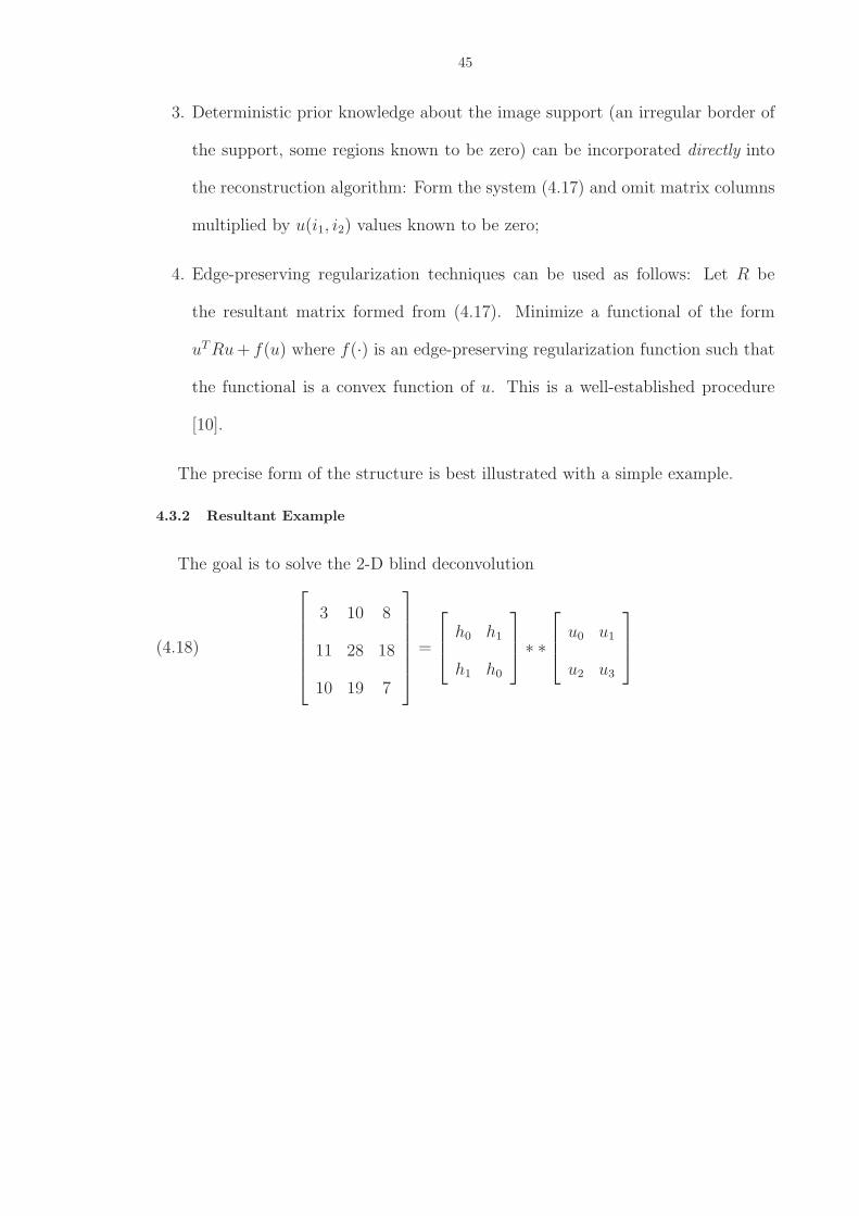
45

3. Deterministic prior knowledge about the image support (an irregular border of

the support, some regions known to be zero) can be incorporated directly into

the reconstruction algorithm: Form the system (4.17) and omit matrix columns

multiplied by u(i1, i2) values known to be zero;

4. Edge-preserving regularization techniques can be used as follows: Let R be

the resultant matrix formed from (4.17). Minimize a functional of the form

uT Ru + f(u) where f(·) is an edge-preserving regularization function such that

the functional is a convex function of u. This is a well-established procedure

[10].

The precise form of the structure is best illustrated with a simple example.

4.3.2 Resultant Example

The goal is to solve the 2-D blind deconvolution

(4.18)

3 10 8

11 28 18

10 19 7

=

h0 h1

h1 h0

∗ ∗

u0 u1

u2 u3

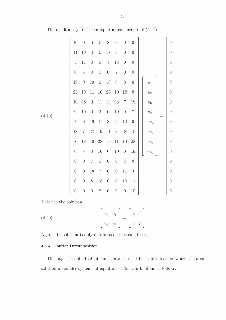
46

The resultant system from equating coefficients of (4.17) is

(4.19)

10 0 0 0 8 0 0 0

11 10 0 0 18 8 0 0

3 11 0 0 7 18 0 0

0 3 0 0 0 7 0 0

19 0 10 0 10 0 8 0

28 19 11 10 28 10 18 8

10 28 3 11 19 28 7 18

0 10 0 3 0 19 0 7

7 0 19 0 3 0 10 0

18 7 28 19 11 3 28 10

8 18 10 28 10 11 19 28

0 8 0 10 0 10 0 19

0 0 7 0 0 0 3 0

0 0 18 7 0 0 11 3

0 0 8 18 0 0 10 11

0 0 0 8 0 0 0 10

u1

u3

u0

u2

−u2

−u0

−u3

−u1

=

0

0

0

0

0

0

0

0

0

0

0

0

0

0

0

0

This has the solution

(4.20)

u0 u1

u2 u3

=

3 4

5 7

Again, the solution is only determined to a scale factor.

4.3.3 Fourier Decomposition

The huge size of (4.20) demonstrates a need for a formulation which requires

solution of smaller systems of equations. This can be done as follows.

47

Let xk = ej2πk/M and yk similarly. Setting y = yk in (4.17) yields

(4.21) Y (x, yk)(xyk)MU(

1

x,

1

yk

) = (xyk)NY (

1

x,

1

yk

)U(x, yk)

Since y(i1, i2) and u(i1, i2) are real, by conjugate symmetry we have U( 1x, 1

yk) =

U∗( 1x∗

, 1y∗

) = U∗( 1x∗

, yk) and similarly for Y (·), since yky∗k = 1. This allows (4.21) to

be rewritten as

(4.22) Y (x, yk)yMk xMU∗(

1

x∗, yk) = yN

k xNY ∗(1

x∗, yk)U(x, yk)

We recognize (4.22) as a decoupled (in k) set of 1-D complex-valued blind deconvo-

lution problems. Each of these can be solved in parallel using any of the methods in

Section 4.2 above.

We can also derive this result directly from the 2-D problem statement (4.16).

Setting y = yk in (4.16) yields

(4.23) Y (x, yk) = H(x, yk)U(x, yk) = H∗(1

x∗, yk)U(x, yk)

from which (4.22) can be derived. And of course we may set x = xk and obtain an

equation like (4.22) with x and y interchanged:

(4.24) Y (xk, y)yMxMk U∗(xk,

1

y∗) = xN

k yNY ∗(xk,1

y∗)U(xk, y)

Still another way to see this quickly is to note that since h(i1, i2) is a real and even

function, its 2-D discrete Fourier transform H(xi, yj) (H(x, y) sampled on the unit

circle) will also be a real and even function. Hence the singly-transformed h(i1, yk)

will also be real and even. This shows most directly why the decoupled 1-D problems

have even PSFs. Of course the FFT may be used to compute quickly Y (x, yk) from

y(i1, i2) and also to compute u(i1, i2) from U(x, yk).

48

4.3.4 Scale Factors

There is still one problem. Each decoupled 1-D problem is only solvable to a scale

factor, as noted in Section 2. Hence (4.22) only yields ckU(x, yk), where ck is the

unknown scale factor for the kth problem. The ck must be determined in order to

recover u(i1, i2).

One way to compute the ck is to make use of the known finite support of u(i1, i2)

and solve the linear system of equations

(4.25a)M∑

k=0

cku(i1, yk)ej 2πM

M+1k = u(i1,M) = 0

(4.25b) u(i1, yk) =M∑

i2=0

u(i1, i2)e−j 2π

M+1i2k

where U(x, y) has now been sampled at yk = ej2πk

M+1 and 0 ≤ i1 ≤ M − 1. This

gives M equations in M + 1 unknowns ck, but the latter are only determined to an

overall scale factor anyways. However, the linear system (4.25a), (4.25b) is dense

and unstructured.

A simpler way is to solve (4.22) for ckU(x, yk) and (4.24) for dkU(xk, y). It is

then a simple matter to read off the relative ratios of the ck from the latter, and

the relative ratios of the dk from the former. There is still an overall scale factor

ambiguity, as expected.

4.3.5 Fourier Example

To illustrate this, we apply (4.22) and (4.24) to the 2-D blind deconvolution

problem (4.18). Since M = 2, we set yk = ±1 and xk = ±1. Setting yk = 1 produces

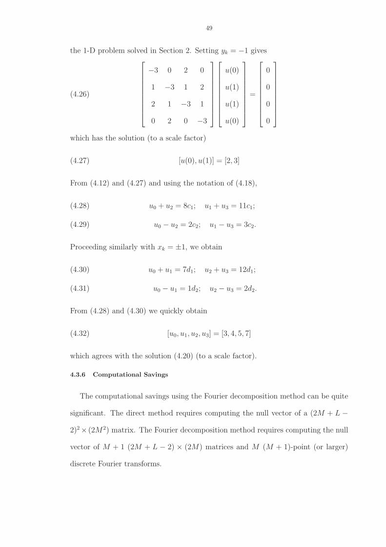
49

the 1-D problem solved in Section 2. Setting yk = −1 gives

(4.26)

−3 0 2 0

1 −3 1 2

2 1 −3 1

0 2 0 −3

u(0)

u(1)

u(1)

u(0)

=

0

0

0

0

which has the solution (to a scale factor)

(4.27) [u(0), u(1)] = [2, 3]

From (4.12) and (4.27) and using the notation of (4.18),

u0 + u2 = 8c1; u1 + u3 = 11c1;(4.28)

u0 − u2 = 2c2; u1 − u3 = 3c2.(4.29)

Proceeding similarly with xk = ±1, we obtain

u0 + u1 = 7d1; u2 + u3 = 12d1;(4.30)

u0 − u1 = 1d2; u2 − u3 = 2d2.(4.31)

From (4.28) and (4.30) we quickly obtain

(4.32) [u0, u1, u2, u3] = [3, 4, 5, 7]

which agrees with the solution (4.20) (to a scale factor).

4.3.6 Computational Savings

The computational savings using the Fourier decomposition method can be quite

significant. The direct method requires computing the null vector of a (2M + L −

2)2 × (2M2) matrix. The Fourier decomposition method requires computing the null

vector of M + 1 (2M + L − 2) × (2M) matrices and M (M + 1)-point (or larger)

discrete Fourier transforms.

50

The number of arithmetic operations required by each of these approaches depends

heavily on the method used. For example, the null vector may be found using the

split algorithm of [87], the multichannel Levinson algorithm, or the inverse power

method. It is clear that savings using the Fourier decomposition method are very

large.

4.4 Noisy Data Case

4.4.1 Formulation

We now consider the noisy data problem. The log-likelihood function is (recall

the assumption of an additive white Gaussian noise field)

(4.33) log pY |U(y|u) = −N2

2log(2πσ2)− 1

2σ2

N−1∑

i1=0

N−1∑

i2=0

[y(i1, i2)−h(i1, i2)∗∗u(i1, i2)]2.

Since the problem is overdetermined, the maximum likelihood estimate (MLE) of

u(i1, i2) is the solution to a 2-D blind deconvolution problem in which the noisy data

y(i1, i2) has been replaced with y(i1, i2). y(i1, i2) has the following two properties:

1. A solution exists to the overdetermined blind deconvolution y(i1, i2) = h(i1, i2)∗

∗u(i1, i2);

2.∑N−1

i1=0

∑N−1i2=0 [y(i1, i2) − y(i1, i2)]

2 is minimized.

That is, we need to find the minimum least-squares norm perturbation of the noisy

data y(i1, i2) to admissible data y(i1, i2) for which a solution to the overdetermined

2-D blind deconvolution problem exists. Then u(i1, i2) is the MLE of u(i1, i2).

Another way to say this is that we need to project the noisy data onto the set of

admissible data for which the overdetermined problem can be solved.

51

4.4.2 Resultant Solution

Fortunately, the formulation (4.17) allows a straightforward solution to this prob-

lem. Since each column of the resultant matrix R consists of the noisy data y(i1, i2)

unwrapped by columns and some zeros (e.g., (18)), we have

(4.34) 2M2

N−1∑

i1=0

N−1∑

i2=0

[y(i1, i2) − y(i1, i2)]2 = ||R − R||2F

where

1. R is the resultant matrix constructed from y(i1, i2);

2. R is the resultant matrix constructed from y(i1, i2);

3. 2M2 comes from the 2M2 columns of R and R;

4. ||A||2F = 1N2

∑Ni=1

∑Nj=1 |Ai,j|2 is the Frobenius or Hilbert-Schmidt matrix norm

of A.

Hence the problem has been reformulated as follows: Compute the minimum Frobe-

nius norm perturbation R of R such that: (1) R keeps the multilevel Toeplitz struc-

ture of R; and (2) R drops rank.

This is a well-know problem in linear algebra. There are at least two known

approaches:

1. Structured total least squares (STLS) [37];

2. Lift-and-project (LAP) [8].

Since these are quite well known we do not review them here. Their relative perfor-

mance on this problem is examined below.

52

4.4.3 Sufficiency Considerations

The above procedure computes an estimate of the image u(i1, i2) that by construc-

tion is M×M . Since the observed blurred image y(i1, i2) is (M +L−1)×(M +L−1),

this does not by itself seem to guarantee that the blurred image is obtained from the

original image by convolution with an L × L PSF h(i1, i2).

The following argument shows that in fact the PSF h(i1, i2) is in fact almost

surely constrained to have L × L support. That is, the procedure recovers not only

an estimate of the image, but an L × L estimate of the PSF, so that it does in fact

find the nearest solution to (1).

First, note that setting y = xN+M−1 in (4.16) unwraps the 2-D problem into

Y (x, x(N+M−1))x(N+M)MU(1

x, (

1

x)(N+M−1)) =

x(N+M)NY (1

x, (

1

x)(N+M−1))U(x, x(N+M−1))

(4.35)

This is known as the Kronecker substitution; it amounts to taking repeated slices

of slope (N + M − 1) through the 2-D wavenumber domain. It effectively unwraps

the 2-D problem into a huge 1-D problem.

The example (4.18) unwraps to the 1-D problem with bands of zeros

{10, 11, 3, 0, 19, 28, 10, 0, 7, 18, 8} =

{h1, h0, 0, 0, h0, h1} ∗ {u2, u0, 0, 0, u3, u1}(4.36)

Equating coefficients in (4.17) and (4.35) show that they both implement the same

equations. This is useful in setting up the system, as follows:

1. Unwrap y(i1, i2) by columns;

2. Insert bands of (M − 1) zeros between each unwrapped column;

3. Form a 1-D resultant matrix with this as its first column, as in Section 4.2;

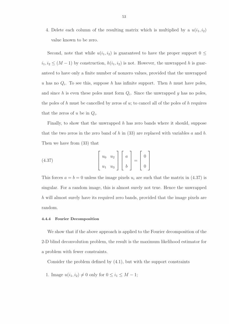
53

4. Delete each column of the resulting matrix which is multiplied by a u(i1, i2)

value known to be zero.

Second, note that while u(i1, i2) is guaranteed to have the proper support 0 ≤

i1, i2 ≤ (M − 1) by construction, h(i1, i2) is not. However, the unwrapped h is guar-

anteed to have only a finite number of nonzero values, provided that the unwrapped

u has no Qi. To see this, suppose h has infinite support. Then h must have poles,

and since h is even these poles must form Qi. Since the unwrapped y has no poles,

the poles of h must be cancelled by zeros of u; to cancel all of the poles of h requires

that the zeros of u be in Qi.

Finally, to show that the unwrapped h has zero bands where it should, suppose

that the two zeros in the zero band of h in (33) are replaced with variables a and b.

Then we have from (33) that

(4.37)

u0 u2

u1 u3

a

b

=

0

0

This forces a = b = 0 unless the image pixels ui are such that the matrix in (4.37) is

singular. For a random image, this is almost surely not true. Hence the unwrapped

h will almost surely have its required zero bands, provided that the image pixels are

random.

4.4.4 Fourier Decomposition

We show that if the above approach is applied to the Fourier decomposition of the

2-D blind deconvolution problem, the result is the maximum likelihood estimator for

a problem with fewer constraints.

Consider the problem defined by (4.1), but with the support constraints

1. Image u(i1, i2) 6= 0 only for 0 ≤ i1 ≤ M − 1;

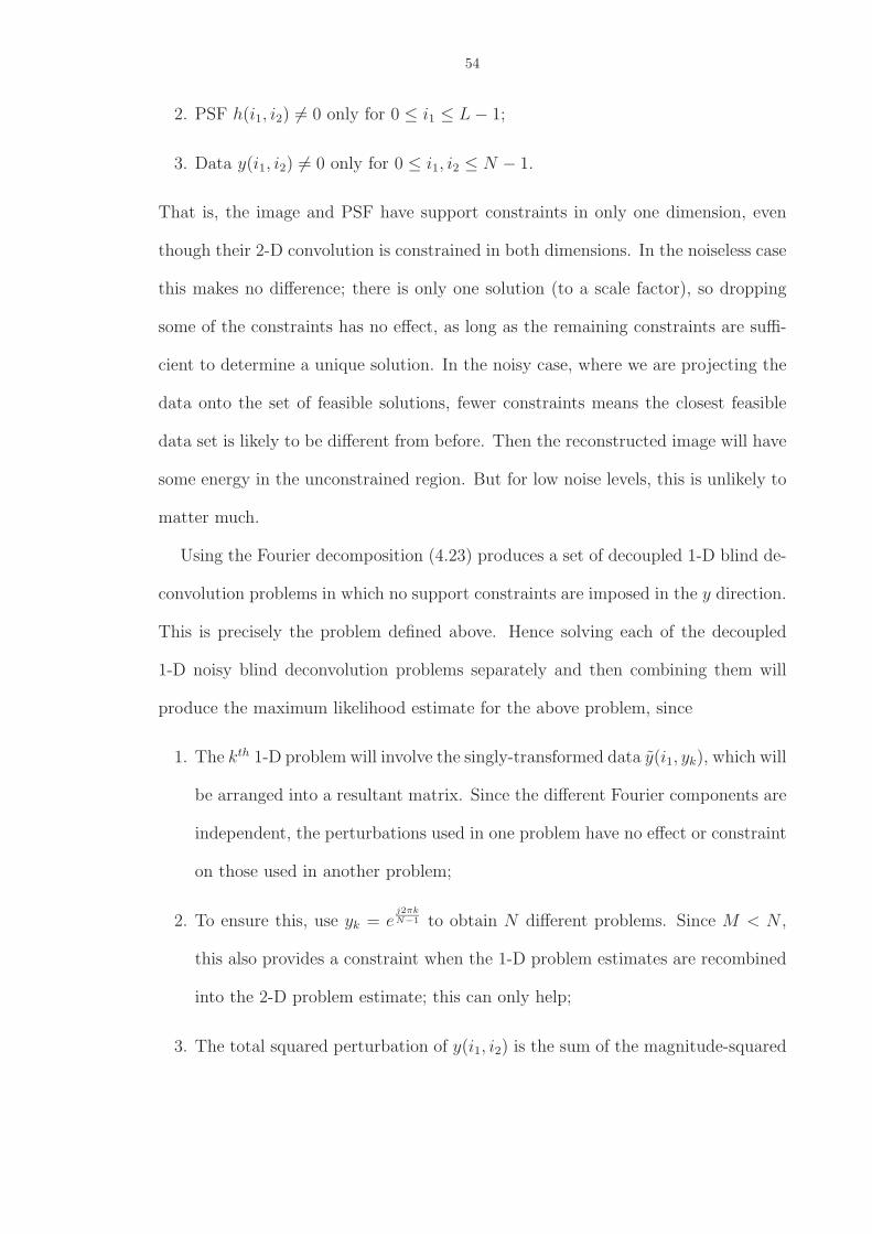
54

2. PSF h(i1, i2) 6= 0 only for 0 ≤ i1 ≤ L − 1;

3. Data y(i1, i2) 6= 0 only for 0 ≤ i1, i2 ≤ N − 1.

That is, the image and PSF have support constraints in only one dimension, even

though their 2-D convolution is constrained in both dimensions. In the noiseless case

this makes no difference; there is only one solution (to a scale factor), so dropping

some of the constraints has no effect, as long as the remaining constraints are suffi-

cient to determine a unique solution. In the noisy case, where we are projecting the

data onto the set of feasible solutions, fewer constraints means the closest feasible

data set is likely to be different from before. Then the reconstructed image will have

some energy in the unconstrained region. But for low noise levels, this is unlikely to

matter much.

Using the Fourier decomposition (4.23) produces a set of decoupled 1-D blind de-

convolution problems in which no support constraints are imposed in the y direction.

This is precisely the problem defined above. Hence solving each of the decoupled

1-D noisy blind deconvolution problems separately and then combining them will

produce the maximum likelihood estimate for the above problem, since

1. The kth 1-D problem will involve the singly-transformed data y(i1, yk), which will

be arranged into a resultant matrix. Since the different Fourier components are

independent, the perturbations used in one problem have no effect or constraint

on those used in another problem;

2. To ensure this, use yk = ej2πk

N−1 to obtain N different problems. Since M < N ,

this also provides a constraint when the 1-D problem estimates are recombined

into the 2-D problem estimate; this can only help;

3. The total squared perturbation of y(i1, i2) is the sum of the magnitude-squared

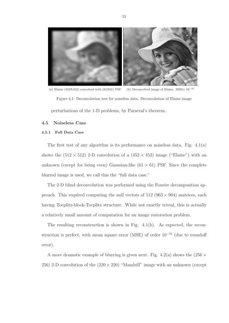
55

(a) Elaine (452X452) convolved with (61X61) PSF (b) Deconvolved image of Elaine. MSE≃ 10−31

Figure 4.1: Deconvolution test for noiseless data. Deconvolution of Elaine image

perturbations of the 1-D problems, by Parseval’s theorem.

4.5 Noiseless Case

4.5.1 Full Data Case

The first test of any algorithm is its performance on noiseless data. Fig. 4.1(a)

shows the (512 × 512) 2-D convolution of a (452 × 452) image (“Elaine”) with an

unknown (except for being even) Gaussian-like (61 × 61) PSF. Since the complete

blurred image is used, we call this the “full data case.”

The 2-D blind deconvolution was performed using the Fourier decomposition ap-

proach. This required computing the null vectors of 512 (963 × 904) matrices, each

having Toeplitz-block-Toeplitz structure. While not exactly trivial, this is actually

a relatively small amount of computation for an image restoration problem.

The resulting reconstruction is shown in Fig. 4.1(b). As expected, the recon-

struction is perfect, with mean square error (MSE) of order 10−31 (due to roundoff

error).

A more dramatic example of blurring is given next. Fig. 4.2(a) shows the (256×

256) 2-D convolution of the (220× 220) “Mandrill” image with an unknown (except

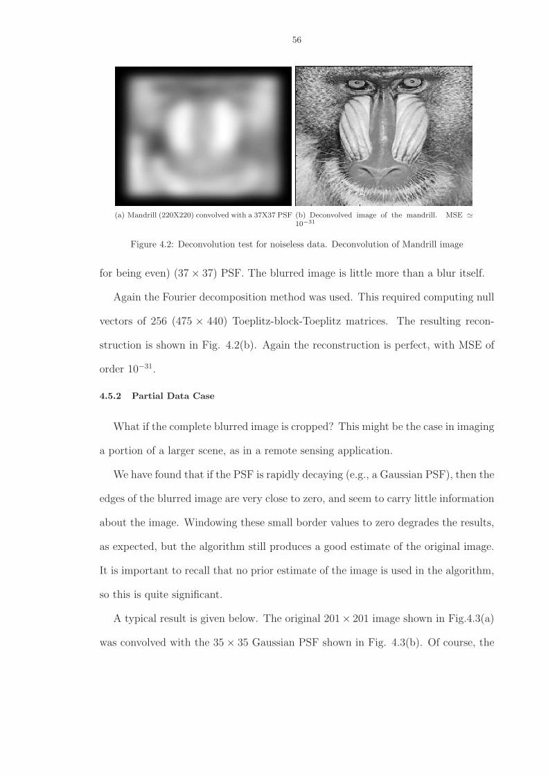
56

(a) Mandrill (220X220) convolved with a 37X37 PSF (b) Deconvolved image of the mandrill. MSE ≃10−31

Figure 4.2: Deconvolution test for noiseless data. Deconvolution of Mandrill image

for being even) (37 × 37) PSF. The blurred image is little more than a blur itself.

Again the Fourier decomposition method was used. This required computing null

vectors of 256 (475 × 440) Toeplitz-block-Toeplitz matrices. The resulting recon-

struction is shown in Fig. 4.2(b). Again the reconstruction is perfect, with MSE of

order 10−31.

4.5.2 Partial Data Case

What if the complete blurred image is cropped? This might be the case in imaging

a portion of a larger scene, as in a remote sensing application.

We have found that if the PSF is rapidly decaying (e.g., a Gaussian PSF), then the

edges of the blurred image are very close to zero, and seem to carry little information

about the image. Windowing these small border values to zero degrades the results,

as expected, but the algorithm still produces a good estimate of the original image.

It is important to recall that no prior estimate of the image is used in the algorithm,

so this is quite significant.

A typical result is given below. The original 201× 201 image shown in Fig.4.3(a)

was convolved with the 35 × 35 Gaussian PSF shown in Fig. 4.3(b). Of course, the

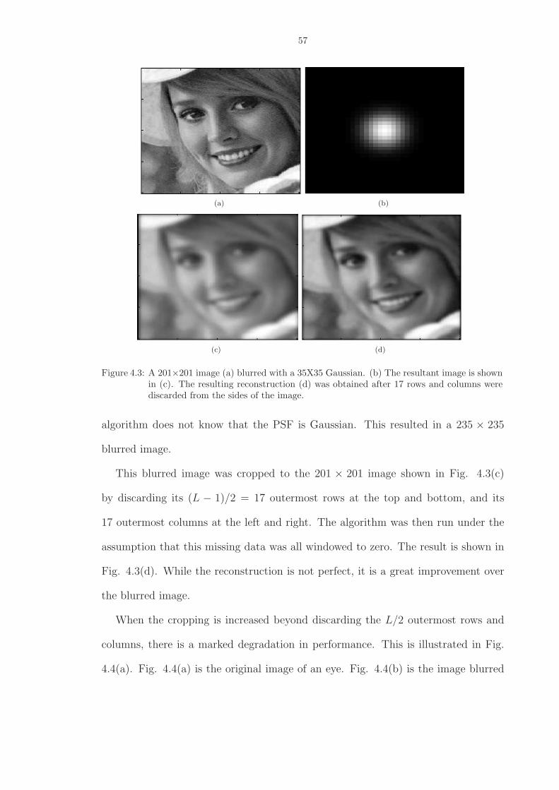
57

(a) (b)

(c) (d)

Figure 4.3: A 201×201 image (a) blurred with a 35X35 Gaussian. (b) The resultant image is shownin (c). The resulting reconstruction (d) was obtained after 17 rows and columns werediscarded from the sides of the image.

algorithm does not know that the PSF is Gaussian. This resulted in a 235 × 235

blurred image.

This blurred image was cropped to the 201 × 201 image shown in Fig. 4.3(c)

by discarding its (L − 1)/2 = 17 outermost rows at the top and bottom, and its

17 outermost columns at the left and right. The algorithm was then run under the

assumption that this missing data was all windowed to zero. The result is shown in

Fig. 4.3(d). While the reconstruction is not perfect, it is a great improvement over

the blurred image.

When the cropping is increased beyond discarding the L/2 outermost rows and

columns, there is a marked degradation in performance. This is illustrated in Fig.

4.4(a). Fig. 4.4(a) is the original image of an eye. Fig. 4.4(b) is the image blurred

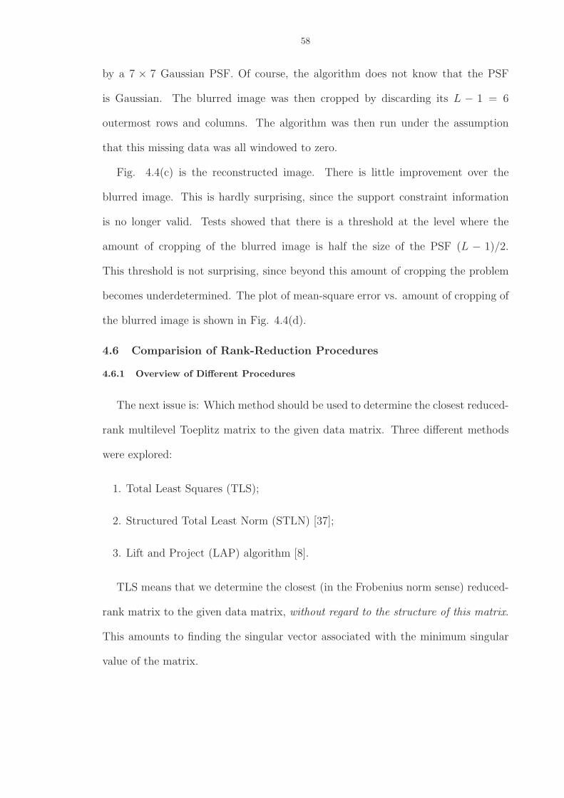
58

by a 7 × 7 Gaussian PSF. Of course, the algorithm does not know that the PSF

is Gaussian. The blurred image was then cropped by discarding its L − 1 = 6

outermost rows and columns. The algorithm was then run under the assumption

that this missing data was all windowed to zero.

Fig. 4.4(c) is the reconstructed image. There is little improvement over the

blurred image. This is hardly surprising, since the support constraint information

is no longer valid. Tests showed that there is a threshold at the level where the

amount of cropping of the blurred image is half the size of the PSF (L − 1)/2.

This threshold is not surprising, since beyond this amount of cropping the problem

becomes underdetermined. The plot of mean-square error vs. amount of cropping of

the blurred image is shown in Fig. 4.4(d).

4.6 Comparision of Rank-Reduction Procedures

4.6.1 Overview of Different Procedures

The next issue is: Which method should be used to determine the closest reduced-

rank multilevel Toeplitz matrix to the given data matrix. Three different methods

were explored:

1. Total Least Squares (TLS);

2. Structured Total Least Norm (STLN) [37];

3. Lift and Project (LAP) algorithm [8].

TLS means that we determine the closest (in the Frobenius norm sense) reduced-

rank matrix to the given data matrix, without regard to the structure of this matrix.

This amounts to finding the singular vector associated with the minimum singular

value of the matrix.

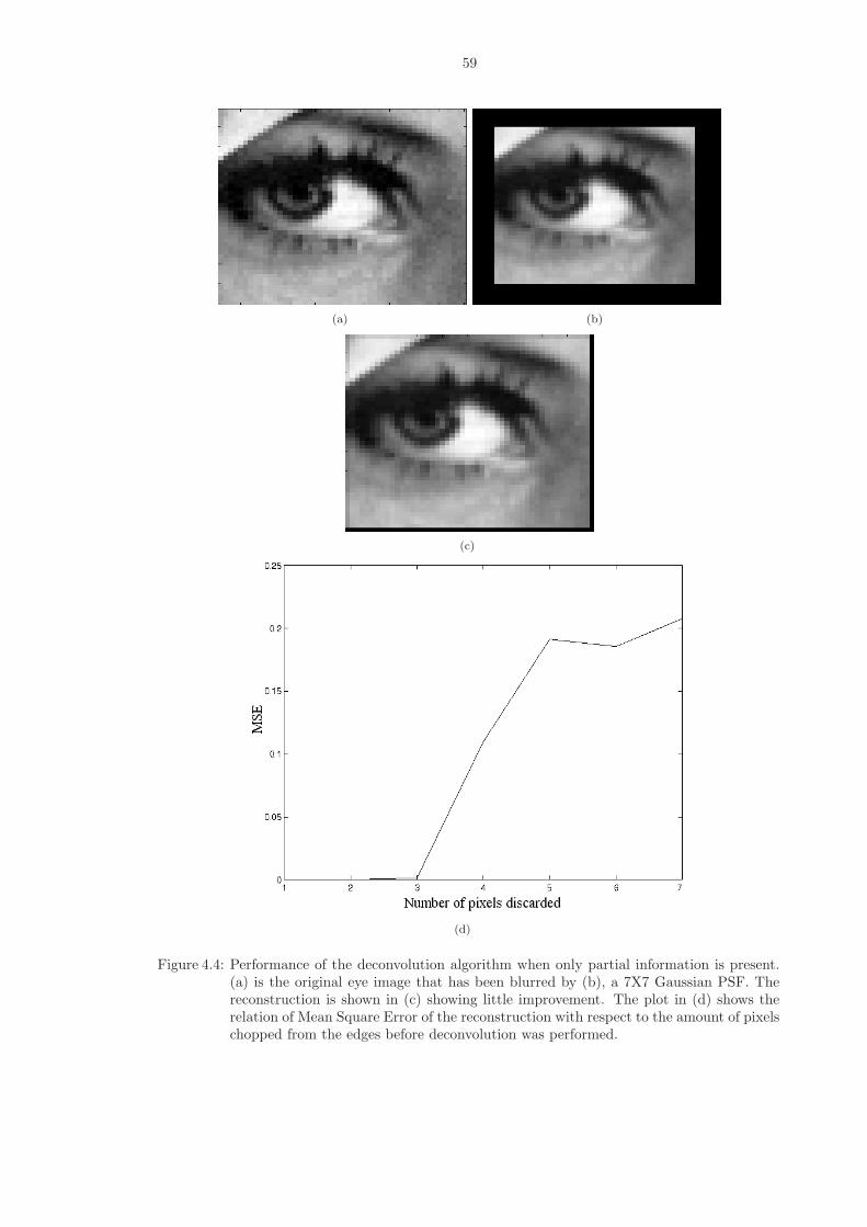
59

(a) (b)

(c)

(d)

Figure 4.4: Performance of the deconvolution algorithm when only partial information is present.(a) is the original eye image that has been blurred by (b), a 7X7 Gaussian PSF. Thereconstruction is shown in (c) showing little improvement. The plot in (d) shows therelation of Mean Square Error of the reconstruction with respect to the amount of pixelschopped from the edges before deconvolution was performed.

60

STLN is an incremental method in which the matrix is incrementally perturbed

toward a reduced-rank matrix, while maintaining its multilevel Toeplitz structure

[37].

LAP is an iterative procedure which works as follows [8]. First, the closest matrix

(in the Frobenius norm sense) is found using TLS. Next, the matrix is then averaged

along its diagonals (this is also known as Toeplitzation). The process is repeated

until the increments in the solution are reduced to a preset tolerance.

The tolerance for STLN was set at ǫ = 10−8 with a limit of 100 iterations and

ℓ2 norm minimization. Least squares was used to solve the linear problem at each

step. The conjugate gradient least squares (CGLS) method [63] was also tried for

solving the linear problem encountered in each iteration of STLN. However, CGLS

was found to be very time consuming and did not provide much improvement over

least squares minimization when used in STLN.

All simulations were peformed using Matlab. Regularization tools developed for

Matlab were also used [25].

4.6.2 Direct Method

The Direct Method is the method of Section III, without Fourier decomposition.

Accordingly, only small images were used, in order to conduct an extensive numerical

investigation.

A (4×4) test image was generated using linspace.m and convolved with a (2×2)

even PSF. Zero-mean Gaussian white nose was added with SNRs varying from 0-55

dB. At every noise level, 100 noise realizations were used.

Results are given in Table 4.1. Note that STLN outperformed both LAP and TLS

at high noise levels. However, TLS gave the best results at low noise levels. Even at

high SNRs, STLN produced MSE≈ 0.001.

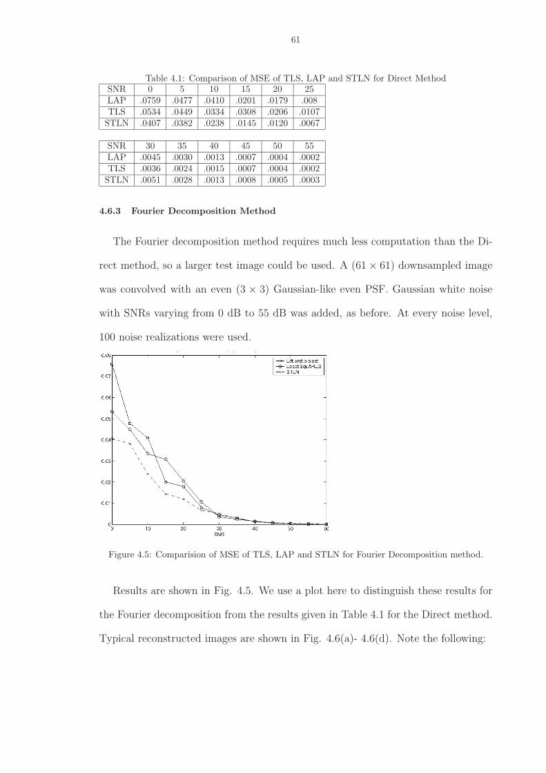
61

Table 4.1: Comparison of MSE of TLS, LAP and STLN for Direct MethodSNR 0 5 10 15 20 25LAP .0759 .0477 .0410 .0201 .0179 .008TLS .0534 .0449 .0334 .0308 .0206 .0107

STLN .0407 .0382 .0238 .0145 .0120 .0067

SNR 30 35 40 45 50 55LAP .0045 .0030 .0013 .0007 .0004 .0002TLS .0036 .0024 .0015 .0007 .0004 .0002

STLN .0051 .0028 .0013 .0008 .0005 .0003

4.6.3 Fourier Decomposition Method

The Fourier decomposition method requires much less computation than the Di-

rect method, so a larger test image could be used. A (61 × 61) downsampled image

was convolved with an even (3 × 3) Gaussian-like even PSF. Gaussian white noise

with SNRs varying from 0 dB to 55 dB was added, as before. At every noise level,

100 noise realizations were used.

Figure 4.5: Comparision of MSE of TLS, LAP and STLN for Fourier Decomposition method.

Results are shown in Fig. 4.5. We use a plot here to distinguish these results for

the Fourier decomposition from the results given in Table 4.1 for the Direct method.

Typical reconstructed images are shown in Fig. 4.6(a)- 4.6(d). Note the following:

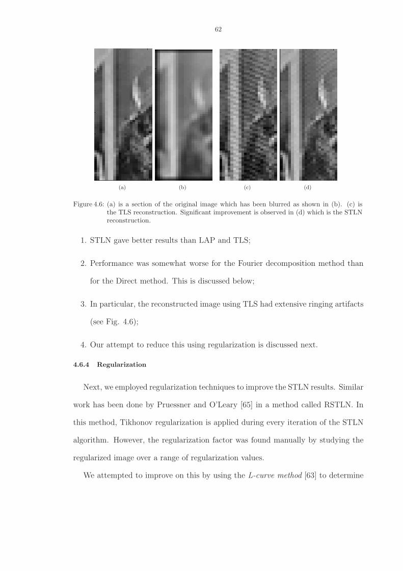
62

(a) (b) (c) (d)

Figure 4.6: (a) is a section of the original image which has been blurred as shown in (b). (c) isthe TLS reconstruction. Significant improvement is observed in (d) which is the STLNreconstruction.

1. STLN gave better results than LAP and TLS;

2. Performance was somewhat worse for the Fourier decomposition method than

for the Direct method. This is discussed below;

3. In particular, the reconstructed image using TLS had extensive ringing artifacts

(see Fig. 4.6);

4. Our attempt to reduce this using regularization is discussed next.

4.6.4 Regularization

Next, we employed regularization techniques to improve the STLN results. Similar

work has been done by Pruessner and O’Leary [65] in a method called RSTLN. In

this method, Tikhonov regularization is applied during every iteration of the STLN

algorithm. However, the regularization factor was found manually by studying the

regularized image over a range of regularization values.

We attempted to improve on this by using the L-curve method [63] to determine

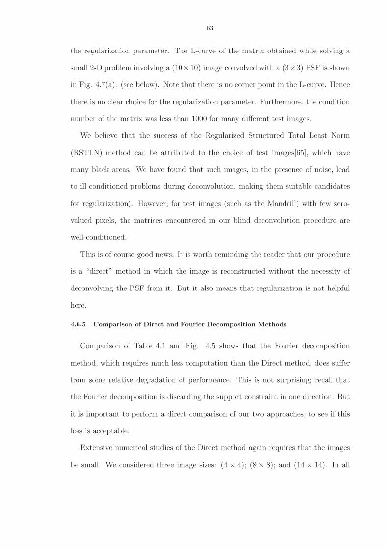
63

the regularization parameter. The L-curve of the matrix obtained while solving a

small 2-D problem involving a (10×10) image convolved with a (3×3) PSF is shown

in Fig. 4.7(a). (see below). Note that there is no corner point in the L-curve. Hence

there is no clear choice for the regularization parameter. Furthermore, the condition

number of the matrix was less than 1000 for many different test images.

We believe that the success of the Regularized Structured Total Least Norm

(RSTLN) method can be attributed to the choice of test images[65], which have

many black areas. We have found that such images, in the presence of noise, lead

to ill-conditioned problems during deconvolution, making them suitable candidates

for regularization). However, for test images (such as the Mandrill) with few zero-

valued pixels, the matrices encountered in our blind deconvolution procedure are

well-conditioned.

This is of course good news. It is worth reminding the reader that our procedure

is a “direct” method in which the image is reconstructed without the necessity of

deconvolving the PSF from it. But it also means that regularization is not helpful

here.

4.6.5 Comparison of Direct and Fourier Decomposition Methods

Comparison of Table 4.1 and Fig. 4.5 shows that the Fourier decomposition

method, which requires much less computation than the Direct method, does suffer

from some relative degradation of performance. This is not surprising; recall that

the Fourier decomposition is discarding the support constraint in one direction. But

it is important to perform a direct comparison of our two approaches, to see if this

loss is acceptable.

Extensive numerical studies of the Direct method again requires that the images

be small. We considered three image sizes: (4 × 4); (8 × 8); and (14 × 14). In all

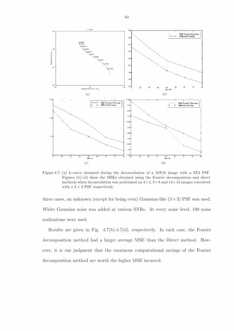
64

10−1

100

101

10−2

10−1

100

101

22.2259

11.5621

6.0147

3.1289

1.6277

0.84674

0.44048

0.22914

0.11920.06201

residual norm || A x − b ||2

solu

tion

norm

|| x

||2

L−curve

(a) (b)

(c) (d)

Figure 4.7: (a) L-curve obtained during the deconvolution of a 10X10 image with a 3X3 PSF.Figures (b)-(d) show the MSEs obtained using the Fourier decomposition and directmethods when deconvolution was performed on 4×4, 8×8 and 14×14 images convolvedwith a 3 × 3 PSF respectively.

three cases, an unknown (except for being even) Gaussian-like (3×3) PSF was used.

White Gaussian noise was added at various SNRs. At every noise level, 100 noise

realizations were used.

Results are given in Fig. 4.7(b)-4.7(d), respectively. In each case, the Fourier

decomposition method had a larger average MSE than the Direct method. How-

ever, it is our judgment that the enormous computational savings of the Fourier

decomposition method are worth the higher MSE incurred.

65

4.7 Conclusion

We have formulated the single-channel 2-D blind deconvolution problem with

an even PSF as a linear algebra problem in which the unknown image pixel values

are components of the null vector of a Toeplitz-block-Toeplitz matrix of the observed

blurred image. Hence the image is found directly; it need not be deconvolved from its

blurred version. Two different methods were proposed: one solved the 2-D problem

directly; the other decomposed the problem into multiple decoupled smaller 1-D

problems. The latter method requires much less computation, but it also has a larger

MSE in noise. Our judgment is that the latter method is nonetheless preferable.

Several numerical tests were performed. These included perfect noiseless recon-

struction of large (e.g., (452× 452)) images and comparison of the above two meth-

ods for several different image sizes. Furthermore, three linear algebraic methods for

computing the nearest reduced-rank Toeplitz-block-Toeplitz matrix to the given data

matrix were compared. It was found that STLN seems to work better than LAP or

TLS except in the very low noise level case, in which case TLS worked best (and also

required the least amount of computation). However, at lower SNRs, TLS not only

gave poorer results but also produced reconstructed images with ringing artifacts.

Attempts to correct this with regularization were not successful, and reasons for this

were given. We also noted that the partial data case in which a cropped version of

the blurred image is used still gave results that were a great improvement over the

blurred image.

We have extended the results of this paper to the 3-D case[88]. The scale factor

problem becomes much more significant and difficult in the 3-D case, enough so that

separate publication is warranted.

CHAPTER V

3-D blind deconvolution of even point-spread functions from

compact support images

5.1 Introduction

3-D blind deconvolution refers to the reconstruction of a 3-D image with compact

support from its 3-D convolution with an unknown blurring or point spread function.

This problem arises frequently in optical sectioning microscopy. Though normally

used for deblurring wide-field images it is increasingly being used for improving the

resolution of images obtained from confocal microscopy.

In applications such as microscopy where the images are optical in nature, the

point-spread function may be assumed to be symmetric i.e. an even function of

spatial variables. This is due to reciprocity i.e., an even function of its spatial vari-

ables. This is due to reciprocity;if an excitation at spatial position xo produces a

given electromagnetic field at yo,then the same excitation at yo should produce the

same electromagnetic field at xo. If the Green’s function is translation-invariant

(G(xo, yo) = G(xo − yo)),then G(xo − yo) = G(yo − xo) and G(·) is an even function.

Since both the image and the point-spread function can be assumed to have

finite spatial extent (i.e., finite support), their Fourier transforms may be sampled

in wavenumber. Most images are approximately bandlimited to the extent that they

may also be sampled spatially as well. This leads to the discrete version of this

66

67

problem, in which a discrete-time image known to have finite spatial extent is to

be reconstructed from its convolution with an also-unknown point-spread function

(PSF).

Current deconvolution techniques used in microscopy include the Lucy-Richardson

method [48, 68], the Ayers-Dainty method [24], ITCM and Carrington methods[81].

Most of these methods are non-blind iterative methods that require thousands of

iterations and are not guaranteed to converge. Methods based on minimization of

a residual require good priors for both the image and the PSF which are often not

available. PSFs are estimated using polystyrene beads in microscopy. However, this

is a tedious task prone to measurement error [55]. These difficulties motivate the

use of non-iterative blind deconvolution methods such as the one described in this

paper.

5.1.1 Problem Formulaton

The 3-D discrete blind deconvolution problem is as follows [41]. We observe

(5.1) y(i1, i2, i3) = h(i1, i2, i3) ∗ ∗ ∗ u(i1, i2, i3) + n(i1, i2, i3)

where ∗ ∗ ∗ denotes convolutions in i1, i2 and i3. The 1-D convolution ∗ is defined

here as

(5.2) h(n) ∗ u(n) =n∑

i=0

h(n − i)u(i) =n∑

i=0

h(i)u(n − i).

We make the following assumptions:

1. u(i1, i2, i3) 6= 0 only for 0 ≤ i1, i2, i3 ≤ M − 1;

2. h(i1, i2, i3) 6= 0 only for 0 ≤ i1, i2, i3 ≤ L − 1;

3. y(i1, i2, i3) 6= 0 only for 0 ≤ i1, i2, i3 ≤ N − 1;

68

4. h(i1, i2, i3) = h(L − i1, L − i2, L − i3) (even PSF); N = L + M − 1;

5. n(i1, i2, i3) is a zero-mean white Gaussian noise random field;

6. All quantities are real functions.

Given knowledge of only the data y(i1, i2, i3), the goal is to reconstruct the im-

age u(i1, i2, i3) and point-spread function (PSF) h(i1, i2, i3); hence the term “blind

deconvolution.” No stochastic assumptions are made about either the image or the

point-spread function. This precludes use of methods based on cumulants, ARMA

or Poisson image models or stochastic equalization.

In many applications, only partial information about Y (i1, i2, i3) is available. For

example:

Y (i1, i2, i3), 0 ≤ i1, i2, i3 ≤ M − 1

i.e. the size of the blur image is the same as that of the original image. We will show

that even in this case, good results are sometimes obtained using our method.

The problem addressed in this paper should be distinguished from the problem of

multiple-blur blind deconvolution, which has been addressed in many recent papers.

In the latter problem, a single unknown signal or image is filtered with several un-

known blurring functions, resulting in several known outputs. This is conceptually

a much simpler problem than the single-blur blind deconvolution problem.

5.1.2 Problem Ambiguities

There are three trivial ambiguities to the 3-D blind deconvolution problem:

1. Scale factor: If {h(i1, i2, i3), u(i1, i2, i3)} is a solution, then {ch(i1, i2, i3),1cu(i1, i2, i3)}

is also a solution for any real constant c. If c cannot be determined from the

image energy, it usually is irrelevant. We consider the problem to be solved

when the image is determined to a scale factor.

69

2. Translation: If {h(i1, i2, i3), u(i1, i2, i3)} is a solution, then {h(i1+d1, i2+d2, i3+

d3), u(i1 − d1, i2 − d2, i3 − d3)} is also a solution for any constants d1, d2, d3. We

eliminate this ambiguity by specifying the supports in (2).

3. Exchange: We need to be able to distinguish h(i1, i2, i3) from u(i1, i2, i3). Since

h(i1, i2, i3) is an even function by assumption, this requires that the image not

also be an even function, or that L 6= M .

We assume that the 3-D z-transforms

(5.3) H(x, y, z) =L−1∑

i1=0

L−1∑

i2=0

L−1∑

i3=0

h(i1, i2, i3)xyz−i1−i2−i3

and

(5.4) U(x, y, z) =M−1∑

i1=0

M−1∑

i2=0

M−1∑

i3=0

u(i1, i2, i3)xyz−i1−i2−i3

are irreducible (they cannot be factored). This is almost surely true [44]. One way

to see this quickly is to note that in the noiseless case, (5.1) is N3 = (L + M −

1)3 simultaneous quadratic equations in L3 + M3 unknowns. Since the problem

is overdetermined, by Bezout’s theorem there is almost surely no more than one

solution. In fact, there are generically no solutions; only from (5.1) do we know that

there is a perturbation of the data for which a solution exists.

5.2 2-D and 3-D Solution

5.2.1 2-D Solution

It is essential to understand the solution of the 1-D and 2-D problem to understand

the solution of the 3-D problem. We shall review noiseless 2-D blind deconvolution

first. The 2-D solution is an extension of the 1-D solution [71].

70

Taking 2-D z-transform of the noiseless 2-D version of (5.1) yields

(5.5) Y (z1, z2) = H(z1, z2)U(z1, z2) = (z1z2)LH(

1

z1

,1

z2

)U(z1, z2)

since h(i1, i2) = h(L − i1, L − i2). This leads to

(5.6) Y (z1, z2)(z1, z2)MU(

1

z1

,1

z2

) = (z1z2)NY (

1

z1

,1

z2

)U(z1, z2)

Equating coefficients leads to a block Toeplitz matrix with Toeplitz blocks. This

is known as Toeplitz block Toeplitz or multilevel Toeplitz structure. The matrix

is formed by nesting the Toeplitz matrices that implement 1D convolutions. The

matrix size is

(5.7) (N + M − 1)2 × (2M2) = (2M + L − 2)2 × (2M2)

.

The matrix is overdetermined if L > 2. However, the overdetermination is much

greater than in the 1-D case. The 2-D problem is best understood with an example.

5.2.2 Fourier Decomposition in 2-D

The 2-D problem is solved by solving a system of equations of a block Toeplitz

matrix whose size is given by (5.7). This matrix quickly grows in size, even for small

problems. For instance: If M = 5 and L = 3, then the size of the matrix is 121× 50.

The huge size of these matrices demonstrate the need for a formulation that can

decouple this large system of equations into smaller systems. This can be done as

follows.

Let xk = ej2πk/M and yk be similarly defined. Setting z2 = yk in (5.6) yields

(5.8) Y (z1, yk)(z1yk)MU(

1

z1

,1

yk

) = (z1yk)NY (

1

z1

,1

yk

)U(z1, yk)

71

Since y(i1, i2) and u(i1, i2) are real, conjugate symmetry allows (5.8) to be rewritten

as

(5.9) Y (z1, yk)yMk zM

1 U∗(1

z∗1, yk) = yN

k zN1 Y ∗(

1

z∗1, yk)U(z1, yk)

since |yk| = 1. We recognize (5.9) as a decoupled (in k) set of 1-D complex-valued

blind deconvolution problems. Each of these can be solved in parallel.

Another way to see this quickly is to note that since h(i1, i2) is a real and even

function, its 2-D discrete Fourier transform H(z1i, z1j) (H(z1, z2) sampled on the unit

circle) will also be a real and even function. Hence the singly-transformed h(i1, yk)

will also be real and even. This shows most directly why the decoupled 1-D problems

have even PSFs. Of course the FFT may be used to compute quickly Y (z1, yk) from

y(i1, i2) and also to compute u(i1, i2) from U(z1, yk).

5.2.3 Scale Factors in 2-D

The problem is not completely solved yet. Each decoupled 1-D problem is only

solvable to a scale factor. Hence (5.9) only yields ckU(x, yk), where ck is the unknown

scale factor for the kth problem. The ck must be determined in order to recover

u(i1, i2).

The easiest way is to solve (5.9) for ckU(x, yk) and (23) for dkU(xk, y). We then

read off the relative ratios of the ck from the latter, and the relative ratios of the dk

from the former. There is still an overall scale factor ambiguity, as expected.

5.2.4 3-D Blind Deconvolution

We now specify our new procedure for 3-D blind deconvolution. All of the results

to follow are new.

The 3-D analogue to (5.5) is

72

(5.10) Y (z1, z2, z3) = H(z1, z2, z3)U(z1, z2, z3) = (z1z2z3)LH(

1

z1

,1

z2

,1

z3

)U(z1, z2, z3)

This leads to

(5.11) Y (z1, z2, z3) = (z1z2z3)MU(

1

z1

,1

z2

,1

z3

) = (z1z2z3)NY (

1

z1

,1

z2

,1

z3

)U(z1, z2, z3)

Equating coefficients would result in a doubly nested Toeplitz matrix. The matrix

size is now (N + M − 1)3 × (2M3) = (2M + L − 2)3 × (2M)3. If M = 8 and L = 3

then the matrix would be 4913 × 1024 in size. It is evident that without Fourier

decomposition, 3-D blind deconvolution would be impractical using this approach.

5.2.5 Fourier Decomposition in 3-D

Let xk = ej2πk/M and yk and zk be similarly defined. Setting y = yk in (5.11)

yields

(5.12) Y (z1, yk, z3)(z1ykz3)MU(

1

z1

,1

yk

,1

z3

) = (z1ykz3)NY (

1

z1

,1

yk

,1

z3

)U(z1, yk, z3)

Conjugate symmetry allows us to rewrite the above equation as

(5.13) Y (z1, yk, z3)(z1ykz3)MU∗(

1

z∗1,

1

yk

,1

z∗3) = (z1ykz3)

NY ∗(1

z∗1,

1

yk

,1

z∗3)U(z1, yk, z3)

We recognize the above equation as a coupled set of 2-D problems. Each of these

2-D problems can further be solved by decoupling them into a set of 1D problems as

shown before. The same can be done by substituting z1 = xk or z3 = zk, leading to

the following expressions.

(5.14) Y (xk, z2, z3)(xkz2z3)MU∗(

1

xk

,1

z∗2,

1

z∗3) = (xkz2z3)

NY ∗(1

xk

,1

z∗2,

1

z∗3)U(xk, z2, z3)

73

(5.15) Y (z1, z2, zk)(z1z2zk)MU∗(

1

z∗1,

1

z∗2,

1

zk

) = (z1z2zk)NY ∗(

1

z∗1,

1

z∗2,

1

zk

)U(z1, z2, zk)

5.2.6 Scale Factors in 3-D

As in the 2-D case, each decoupled 2-D problem is only solvable to a scale factor.

Hence (5.13) yields ckU(z1, yk, z3). In other words, we have slices of the solutions,

depending on the way in which the 3-D problem was decoupled. Each slice has the

right solution to a scale factor, and hence we have to scale these slices with respect

to a common coefficient.

An easy way to achieve this is to solve (5.13) for ckU(z1, yk, z3), (5.14) for dkU(xk, z2, z3)

and (5.15) for ekU(z1, z2, zk), and read off relative ratios using two of the three given

sets of coefficients. The choice of which two sets to use is arbitrary, and in fact one

could perform all three possible combinations to choose the best possible reconstruc-

tion. This is useful especially when a 3-D image matrix might have a non-trivial

nullspace along a certain direction.

5.2.7 Implementation Issues

Specific to the 3-D case, there are a few implementation issues that we need to

report. 3-D images obtained from microscopy often have many black areas repre-

senting zeros in the digitized format. When we take the 1-D Fourier transform along

a direction, it is quite likely that we obtain a 2-D problem, that has a non-trivial

null space. This causes problems, as one of the assumptions, for solving the 2-D case

is that the nullspace has dimension one.

One way of overcoming this is to add minute quantities of broadband noise (vari-

ance of the order of 10−6 of the signal power levels). This seems to avoid the multi-

dimensional nullspace problem. In practice, there will always be some additive noise

74

[44] anyway, so this is reasonable.

We also note that since the PSF is even and if its size is an even intege0r, then

its 3-D DFT will have zeros at ωk = π To see this consider the 1-D even PSF

h0, h1, h2, h2, h1, h0

Real images often have a zero at ω = π;indeed, there should. If the image is

properly sampled using a DFT of odd order (which does not use ω = π) , then the

problem seems to be avoided.

5.3 Noisy Data Case

5.3.1 Formulation

We now consider the noisy data problem (1). Our approach generalizes the ap-

proach we used in [71] for the 2-D case.The log-likelihood function is

(5.16)

log pY |U(y|u) = −N2

2log(2πσ2)− 1

2σ2

N−1∑

i1=0

N−1∑

i2=0

N−1∑

i3=0

[y(i1, i2, i3)−h(i1, i2, i3)∗∗∗u(i1, i2, i3)]2.

Since the problem is overdetermined, the maximum likelihood estimate (MLE) of

u(i1, i2, i3) is the solution to a 3-D blind deconvolution problem in which the noisy

data y(i1, i2, i3) has been replaced with y(i1, i2, i3). y(i1, i2, i3) has the following two

properties:

1. A solution exists to the overdetermined blind deconvolution problem

y(i1, i2, i3) = h(i1, i2, i3) ∗ ∗ ∗ u(i1, i2, i3)

2.∑N−1

i1=0

∑N−1i2=0

∑N−1i3=0 [y(i1, i2, i3) − y(i1, i2, i3)]

2 is minimized.

That is, we need to find the minimum least-squares norm perturbation of the noisy

data y(i1, i2, i3) to admissible data y(i1, i2, i3) for which a solution to the overde-

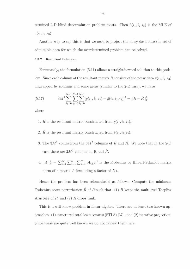
75

termined 2-D blind deconvolution problem exists. Then u(i1, i2, i3) is the MLE of

u(i1, i2, i3).

Another way to say this is that we need to project the noisy data onto the set of

admissible data for which the overdetermined problem can be solved.

5.3.2 Resultant Solution

Fortunately, the formulation (5.11) allows a straightforward solution to this prob-

lem. Since each column of the resultant matrix R consists of the noisy data y(i1, i2, i3)

unwrapped by columns and some zeros (similar to the 2-D case), we have

(5.17) 3M2

N−1∑

i1=0

N−1∑

i2=0

N−1∑

i3=0

[y(i1, i2, i3) − y(i1, i2, i3)]2 = ||R − R||2F

where

1. R is the resultant matrix constructed from y(i1, i2, i3);

2. R is the resultant matrix constructed from y(i1, i2, i3);

3. The 3M2 comes from the 3M2 columns of R and R. We note that in the 2-D

case there are 2M2 columns in R and R.

4. ||A||2F =∑N

i=1

∑Nj=1

∑Nk=1 |Ai,j,k|2 is the Frobenius or Hilbert-Schmidt matrix

norm of a matrix A (excluding a factor of N).

Hence the problem has been reformulated as follows: Compute the minimum

Frobenius norm perturbation R of R such that: (1) R keeps the multilevel Toeplitz

structure of R; and (2) R drops rank.

This is a well-know problem in linear algebra. There are at least two known ap-

proaches: (1) structured total least squares (STLS) [37] ; and (2) iterative projection.

Since these are quite well known we do not review them here.

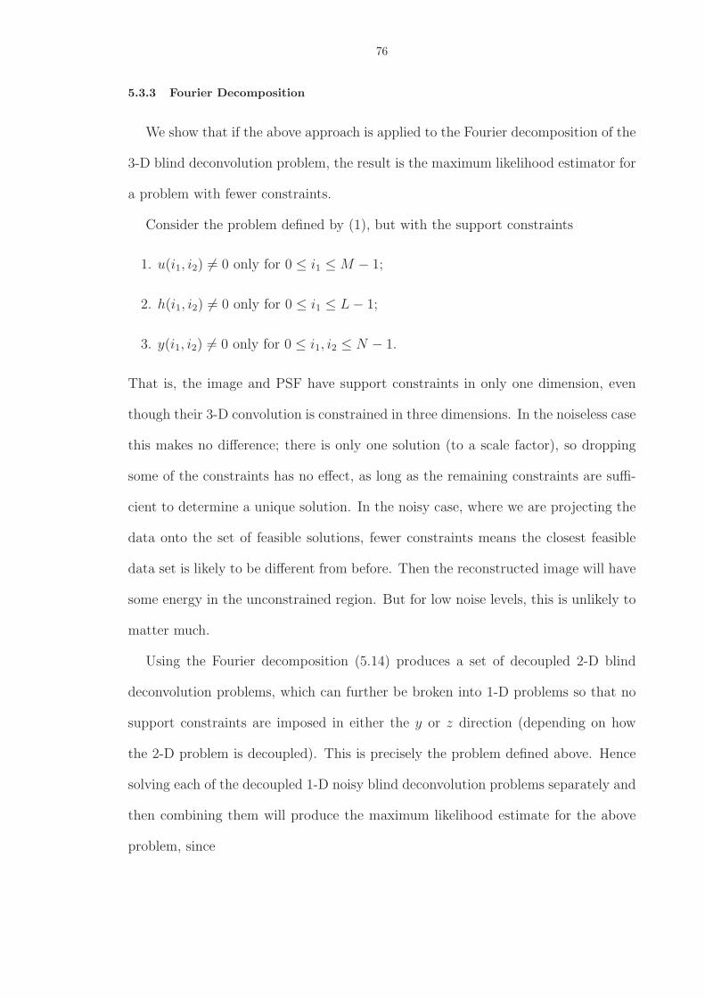
76

5.3.3 Fourier Decomposition

We show that if the above approach is applied to the Fourier decomposition of the

3-D blind deconvolution problem, the result is the maximum likelihood estimator for

a problem with fewer constraints.

Consider the problem defined by (1), but with the support constraints

1. u(i1, i2) 6= 0 only for 0 ≤ i1 ≤ M − 1;

2. h(i1, i2) 6= 0 only for 0 ≤ i1 ≤ L − 1;

3. y(i1, i2) 6= 0 only for 0 ≤ i1, i2 ≤ N − 1.

That is, the image and PSF have support constraints in only one dimension, even

though their 3-D convolution is constrained in three dimensions. In the noiseless case

this makes no difference; there is only one solution (to a scale factor), so dropping

some of the constraints has no effect, as long as the remaining constraints are suffi-

cient to determine a unique solution. In the noisy case, where we are projecting the

data onto the set of feasible solutions, fewer constraints means the closest feasible

data set is likely to be different from before. Then the reconstructed image will have

some energy in the unconstrained region. But for low noise levels, this is unlikely to

matter much.

Using the Fourier decomposition (5.14) produces a set of decoupled 2-D blind

deconvolution problems, which can further be broken into 1-D problems so that no

support constraints are imposed in either the y or z direction (depending on how

the 2-D problem is decoupled). This is precisely the problem defined above. Hence

solving each of the decoupled 1-D noisy blind deconvolution problems separately and

then combining them will produce the maximum likelihood estimate for the above

problem, since

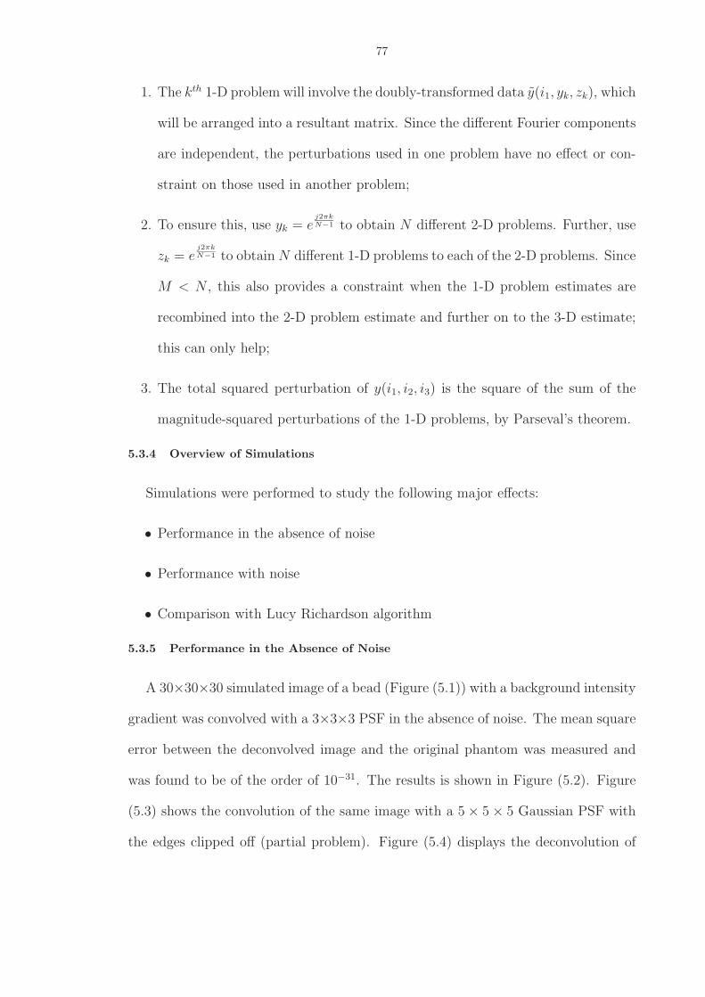
77

1. The kth 1-D problem will involve the doubly-transformed data y(i1, yk, zk), which

will be arranged into a resultant matrix. Since the different Fourier components

are independent, the perturbations used in one problem have no effect or con-

straint on those used in another problem;

2. To ensure this, use yk = ej2πk

N−1 to obtain N different 2-D problems. Further, use

zk = ej2πk

N−1 to obtain N different 1-D problems to each of the 2-D problems. Since

M < N , this also provides a constraint when the 1-D problem estimates are

recombined into the 2-D problem estimate and further on to the 3-D estimate;

this can only help;

3. The total squared perturbation of y(i1, i2, i3) is the square of the sum of the

magnitude-squared perturbations of the 1-D problems, by Parseval’s theorem.

5.3.4 Overview of Simulations

Simulations were performed to study the following major effects:

• Performance in the absence of noise

• Performance with noise

• Comparison with Lucy Richardson algorithm

5.3.5 Performance in the Absence of Noise

A 30×30×30 simulated image of a bead (Figure (5.1)) with a background intensity

gradient was convolved with a 3×3×3 PSF in the absence of noise. The mean square

error between the deconvolved image and the original phantom was measured and

was found to be of the order of 10−31. The results is shown in Figure (5.2). Figure

(5.3) shows the convolution of the same image with a 5 × 5 × 5 Gaussian PSF with

the edges clipped off (partial problem). Figure (5.4) displays the deconvolution of

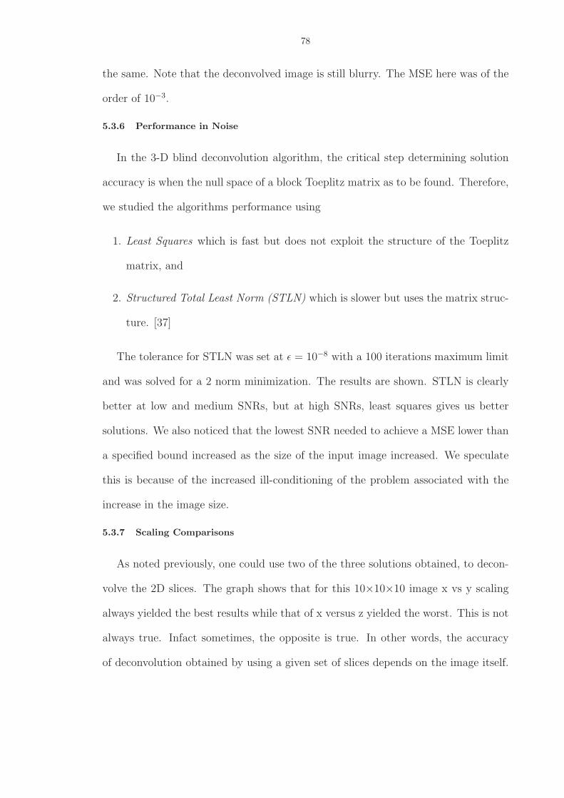
78

the same. Note that the deconvolved image is still blurry. The MSE here was of the

order of 10−3.

5.3.6 Performance in Noise

In the 3-D blind deconvolution algorithm, the critical step determining solution

accuracy is when the null space of a block Toeplitz matrix as to be found. Therefore,

we studied the algorithms performance using

1. Least Squares which is fast but does not exploit the structure of the Toeplitz

matrix, and

2. Structured Total Least Norm (STLN) which is slower but uses the matrix struc-

ture. [37]

The tolerance for STLN was set at ǫ = 10−8 with a 100 iterations maximum limit

and was solved for a 2 norm minimization. The results are shown. STLN is clearly

better at low and medium SNRs, but at high SNRs, least squares gives us better

solutions. We also noticed that the lowest SNR needed to achieve a MSE lower than

a specified bound increased as the size of the input image increased. We speculate

this is because of the increased ill-conditioning of the problem associated with the

increase in the image size.

5.3.7 Scaling Comparisons

As noted previously, one could use two of the three solutions obtained, to decon-

volve the 2D slices. The graph shows that for this 10×10×10 image x vs y scaling

always yielded the best results while that of x versus z yielded the worst. This is not

always true. Infact sometimes, the opposite is true. In other words, the accuracy

of deconvolution obtained by using a given set of slices depends on the image itself.

79

Figure 5.1: 30×30×30 bead image convolved with3×3×3 PSF

Figure 5.2: Deblurred image

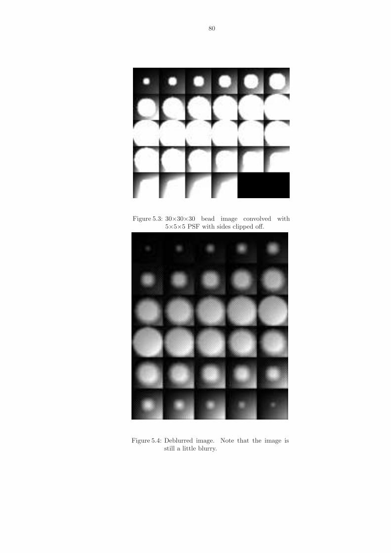
80

Figure 5.3: 30×30×30 bead image convolved with5×5×5 PSF with sides clipped off.

Figure 5.4: Deblurred image. Note that the image isstill a little blurry.

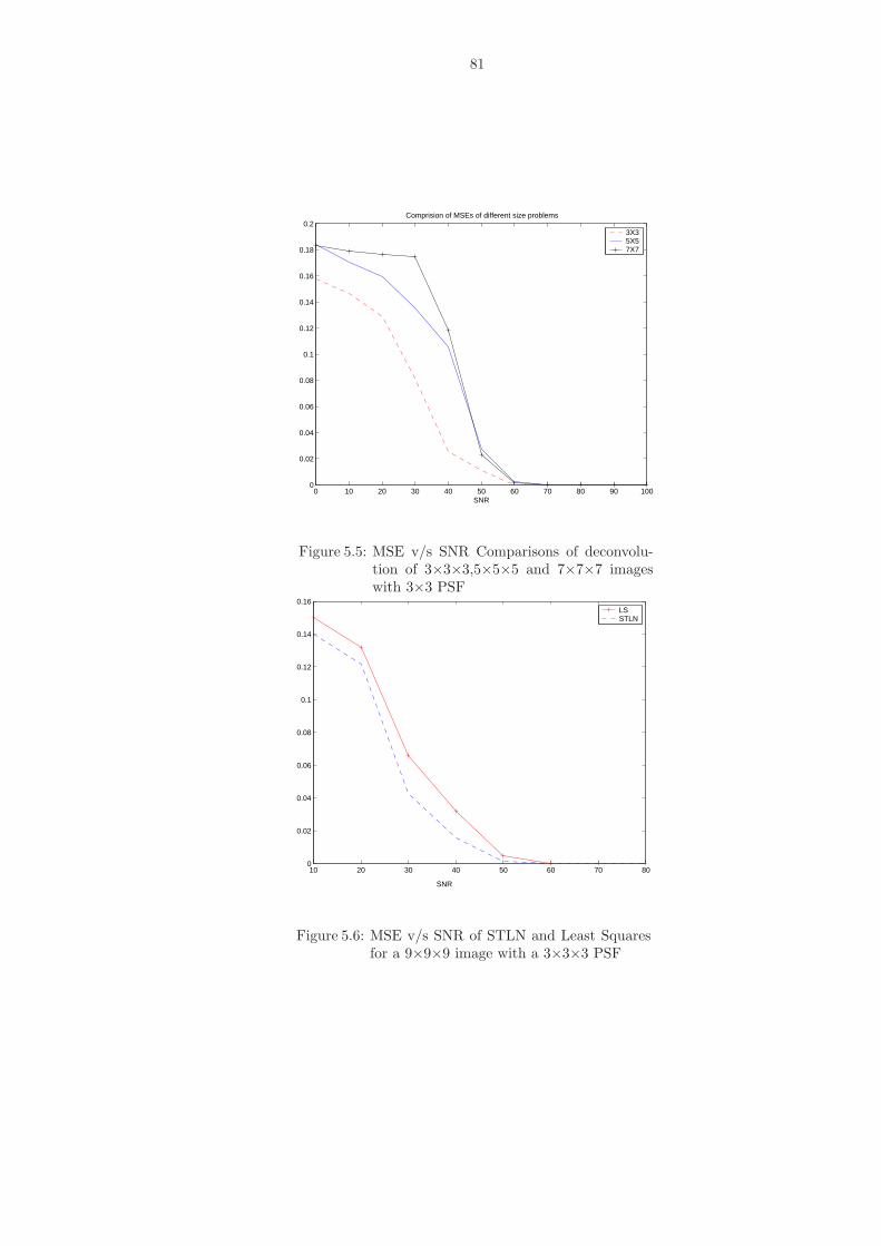
81

0 10 20 30 40 50 60 70 80 90 1000

0.02

0.04

0.06

0.08

0.1

0.12

0.14

0.16

0.18

0.2

SNR

Comprision of MSEs of different size problems

3X35X57X7

Figure 5.5: MSE v/s SNR Comparisons of deconvolu-tion of 3×3×3,5×5×5 and 7×7×7 imageswith 3×3 PSF

10 20 30 40 50 60 70 800

0.02

0.04

0.06

0.08

0.1

0.12

0.14

0.16LSSTLN

SNR

Figure 5.6: MSE v/s SNR of STLN and Least Squaresfor a 9×9×9 image with a 3×3×3 PSF

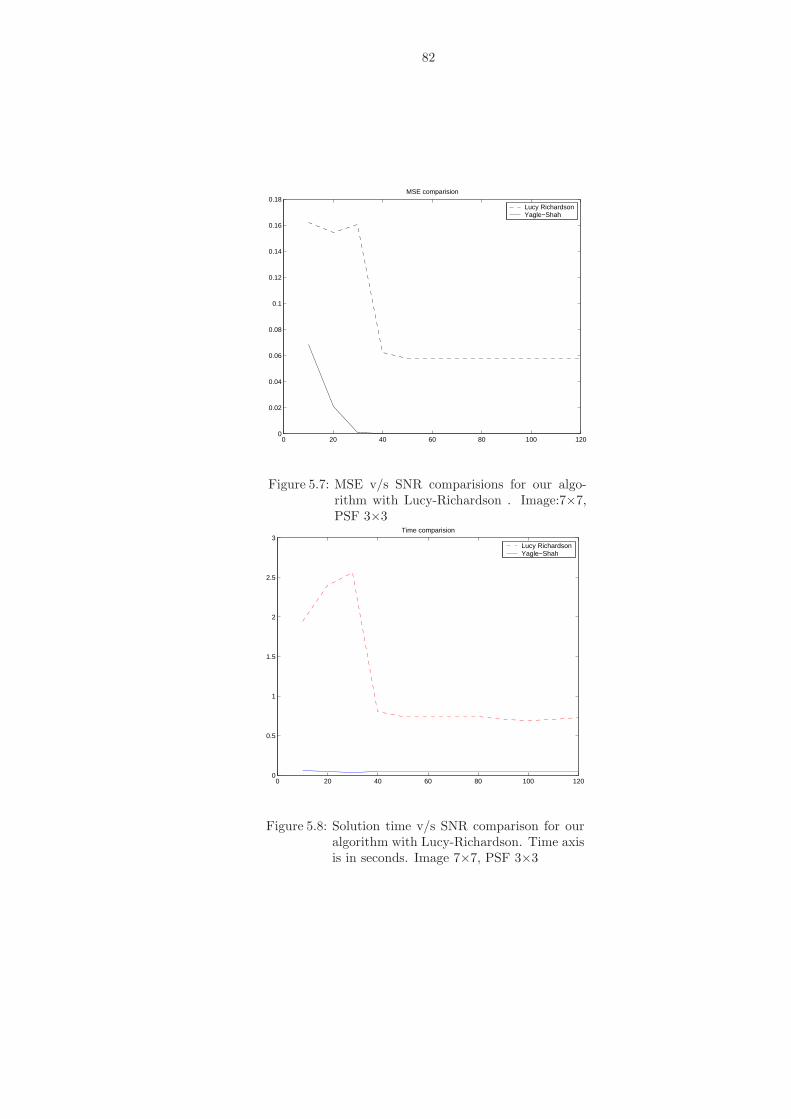
82

0 20 40 60 80 100 1200

0.02

0.04

0.06

0.08

0.1

0.12

0.14

0.16

0.18MSE comparision

Lucy RichardsonYagle−Shah

Figure 5.7: MSE v/s SNR comparisions for our algo-rithm with Lucy-Richardson . Image:7×7,PSF 3×3

0 20 40 60 80 100 1200

0.5

1

1.5

2

2.5

3Time comparision

Lucy RichardsonYagle−Shah

Figure 5.8: Solution time v/s SNR comparison for ouralgorithm with Lucy-Richardson. Time axisis in seconds. Image 7×7, PSF 3×3

83

This is easily understood when one realizes that for an ideal solution one requires

that the resultant matrix be well conditioned when the 1-D Fourier transform of

the 3-D signal is taken along x,y or z. This is easily met for noiseless signals. But

for most real images with lots of zero areas (black areas), the presence of even tiny

amounts of noise makes the problem ill-posed along a certain direction. However,

one could always check to see which scaling yields the best results and hence this is

not a serious problem.

5.3.8 Comparison with Lucy-Richardson Algorithm

To test the effectiveness of the algorithm we compared the 2-D version of the

algorithm to it to the 2-D Lucy-Richardson algorithm for both speed and effectiveness

of deconvolution.

We found that for all the images we tested, our algorithm gave a lower MSE and

also took a much lower time to solve. The figures show two such examples. The

example as shown in Figure (5.7) compares the deconvolution of a 7×7 image with

a 3×3 PSF at different SNRs. The results are averaged over 50 iterations. The time

to solve in seconds is shown in Figure (5.8).

5.4 Conclusions

We have shown that

1. It is possible to formulate 3-D blind deconvolution problems with even point

spread functions as a linear problem in the unknown image pixel values, although

the data are used in a nonlinear manner.

2. In the presence of noise, STLN gives better results than conventional least

squares. In the presence of Gaussian noise; these results are the maximum

likelihood estimates of the original image.

84

3. Fourier decoupling is a very effective tool when solving the deconvolution prob-

lem for large 3-D matrices.

4. Compared to Lucy-Richardson, this algorithm is superior both in terms of the

accuracy of the solution and time needed to solve the problem.

CHAPTER VI

QUILL: A blind deconvolution algorithm for the partial data

problem

6.1 Introduction

6.1.1 Overview

The problem of blind deconvolution has been an active area of research for ap-

proximately the past thirty years [48]. The 2-D version of the problem appears in

areas such as astronomy [40, 41], microscopy [53] and remote sensing [38]. For a good

review of the history and applications of blind deconvolution, we refer the reader to

[44].

2-D deconvolution refers to the problem of reconstructing a 2-D image from its

2-D convolution with a point-spread function (PSF). Often, the PSF is known, or

at least known to a very good approximation. There are several methods to solve

this problem such as Lucy-Richardson [48] or Maximum Entropy deconvolution [60].

However, in many cases the PSF is unknown. This leads to the blind version of the

problem. 2-D blind deconvolution refers to deconvolving the 2-D object from its

convolution with a PSF when the PSF is not known.

Most images are approximately bandlimited to the extent that they may be spa-

tially sampled. This leads to the discrete version of this problem, in which a discrete

image is to be reconstructed from its discrete convolution with an also-unknown dis-

85

86

crete PSF. If the PSF is known, this becomes the solution of an often-ill-conditioned

linear system of equations. When the PSF is unknown, the problem is even harder.

A common approach for blind deconvolution problems is to use an iterative trans-

form algorithm [44, 24] which alternates between spatial and wavenumber domains.

However, these algorithms often stagnate, failing to converge to a solution [24]. An-

other approach, NAS-RIF [45] is guaranteed to converge, but it requires the existence

of a small-support inverse filter.

The problem addressed in this paper should be distinguished from the problem

of multiple-channel blind deconvolution which has received much attention of late

[28, 21, 62, 75]. In this problem, a single unknown signal or image is filtered with

several unknown PSFs resulting in several known outputs. This is conceptually much

simpler than the single blur problem addressed here. To see this quickly, note that

an unknown 1-D signal with compact support can be recovered from its convolutions

with two unknown 1-D PSFs with compact support by simply computing the greatest

common divisor of the z-transforms of the two known convolutions.

6.1.2 The Partial Data Problem

In many applications, such as remote sensing or microscopy, the unknown image

often does not have compact support. Rather, it is just part of a bigger image. The

blurred image that constitutes the data is actually smaller than the image to be

reconstructed. This is called the partial data problem [28].

The difficulty of the partial data problem can be seen by noting that even if the

PSF is known, the image cannot be uniquely determined. This is evident since the

deconvolution problem with an unknown PSF becomes an underdetermined system

of linear equations. We overcome this problem by using an image model that de-

composes the single blur problem to that of a single image with four blurs. By doing

87

this, we will show how a unique solution can be obtained.

6.1.3 New Contributions of This Paper

The specific contributions of this paper to the single-blur partial-data 2-D blind

deconvolution problem are as follows:

1. Solution of the partial data problem requires an image model. We propose a

QUILL (Quincunx-Upsampled Interpolated LinearLy) image model which up-

samples or expands (inserts zeros) into a Quincunx-sampled image, and then

interpolates it using linear splines. This model seems to represent oversampled

images quite well;

2. Using this model, we reformulate the single-blur blind deconvolution problem

as a four-channel multiple-blur blind deconvolution problem, which has been

studied extensively in the literature of late [28, 21, 62, 75];

3. We employ a 2-D version of Bezout’s lemma to enable us to solve for decon-

volvers, rather than the point-spread function itself. Since the reconstructed

image is just a convolution of this deconvolver with the data, our algorithm is a

direct method, effectively reconstructing the image directly without estimating

the PSF and then deconvolving it from the data;

4. We provide several examples, using various types of images and PSFs. This

includes: (1) two real-world images convolved with known PSFs, so that the

reconstructed image can be compared to the true image; and (2) two truly

blind examples in which the algorithm was simply applied directly to real data

of a real-world blurred image; both the PSF and image are unknown.

88

The rest of the paper is organized as follows. Section (6.2) will define the problem

we attempt to solve. Section (6.3) will explain our assumed image model and will

explain its implications and limitations. Section (6.4) will describe the algorithm.

Section (6.5) reports the results we obtained on simulated and actual data. Section

(6.6) concludes with a summary.

6.2 Problem Definition

6.2.1 Problem Assumptions

The 2-D discrete blind deconvolution problem is as follows [44]. We observe

(6.1) y(n1, n2) = h(n1, n2) ∗ ∗u(n1, n2) + n(n1, n2)

where ** represents 2-D convolution.

The 1-D convolution ∗ is defined here as

(6.2) h(n) ∗ u(n) =n∑

i=0

h(n − i)u(i) =n∑

i=0

h(i)u(n − i)

We assume the PSF h(n1, n2) = 0 outside 0 ≤ n1, n2 ≤ L − 1. We do not

assume that the image u(n1, n2) has compact support. The 2-D blind deconvolution

problem is to reconstruct the image u(n1, n2) (and presumably the PSF h(n1, n2))

from the known data y(n1, n2), hence the term “blind deconvolution.” No stochastic

assumptions are made about either the image or the point-spread function. This

precludes use of methods based on cumulants, ARMA or Poisson image models or

stochastic equalization.

To solve the overall 2-D blind deconvolution problem, we partition it into sub-

problems. For each sub-problem, we make the following assumptions:

1. u(n1, n2) = 0 outside 0 ≤ n1, n2 ≤ M − 1;

2. h(n1, n2) = 0 outside 0 ≤ n1, n2 ≤ L − 1;

89

3. y(n1, n2) is known only for L − 1 ≤ n1, n2 ≤ M − 1;

4. n(n1, n2) is a zero-mean 2-D white Gaussian noise random field;

5. All quantities are real-valued.

Note the data y(n1, n2) are known only for L − 1 ≤ n1, n2 ≤ M − 1. This is the

partial data case: no edge information about the image u(n1, n2) is used (the “valid”

convolution). Hence without loss of generality we may set u(n1, n2) = 0 outside

0 ≤ n1, n2 ≤ M − 1.

6.2.2 Problem Ambiguities

There are three trivial ambiguities in the 2-D blind deconvolution problem:

1. Scale factor: If {h(n1, n2), u(n1, n2)} is a solution, then {ch(n1, n2),1cu(n1, n2)}

is also a solution for any real constant c. If c cannot be determined from the

image energy, it usually is irrelevant. We consider the problem to be solved

when the image is determined to a scale factor;

2. Translation: If {h(n1, n2), u(n1, n2)} is a solution, then {h(n1+d1, n2+d2), u(n1−

d1, n2 − d2)} is also a solution for any constants d1, d2. We eliminate this ambi-

guity by specifying the supports above;

3. Exchange: We need to be able to distinguish h(n1, n2) from u(n1, n2). Since we

need M > L above, this is not a problem here.

We also assume that the 2-D z-transforms

H(x, y) =L−1∑

n1=0

L−1∑

n2=0

h(n1, n2)x−n1y−n2(6.3a)

U(x, y) =M−1∑

n1=0

M−1∑

n2=0

u(n1, n2)x−n1y−n2(6.3b)

90

are irreducible (they cannot be factored) for each subproblem. This is almost surely

true [44].

6.3 QUILL Image Model

Sampled images, especially those of large size, tend to be sufficiently lowpass

that they can be approximated by an upsampled or expanded version of the image

convolved with a basis function such as the Haar basis or the linear spline basis. We

shall explain this for the 1-D case.

6.3.1 1-D Image Basis Representation

Consider a discrete 1-D signal u(n). Then, as per our image basis model, we

assume it can be written in the form

(6.4) u(n) =D∑

i=−D

u(2i)φ(n − 2i) = u(n) ∗ φ(n)

where φ(n) is a basis function of duration 4D+1 and

(6.5) u(n) =

u(n) if n is even

0 if n is odd

u(n) is obtained from u(n) by setting u(n) = 0 for odd n. We refer u(n) as the

upsampled or expanded version of u(n) (both terms can be found in various DSP

textbooks).

6.3.2 Specification of the QUILL model

Quincunx sampling refers to the 1-in-4 sampling pattern in images that results in

a checkerboard sampled image [82]. If u(n1, n2) is a 2-D image and u(n1, n2) is its

Quincunx-sampled version, then

91

(6.6) u(n1, n2) =

u(n1, n2) if n1 + n2 is even

0 if n1 + n2 is odd

Consider u(n1, n2). If we (2 × 2) upsample or expand this image along lines

inclined at 45 and 135 degrees, we then get an upsampled or expanded Quincunx

image u2(n1, n2). If u2(n1, n2) is now convolved with a 2-D linear spline basis function

also inclined at 45 and 135 degrees, then this approximation to the original image is

a Quincunx Upsampled Interpolated Linearly (QUILL) image model.

Define the two basis functions

(6.7) φ1(n1, n2) =

0 0 14

0 0

0 12

0 12

0

14

0 1 0 14

0 12

0 12

0

0 0 14

0 0

and

(6.8) φ2(n1, n2) =

0 14

0

14

1 14

0 14

0

Then the Quincunx-sampled u(n1, n2) is

(6.9) u(n1, n2) = u2(n1, n2) ∗ ∗φ1(n1, n2)

Note that u2(n1, n2) has 7/8 of its values equal to zero, while u(n1, n2) has only half

of its values equal to zero.

The QUILL image model u(n1, n2) of u(n1, n2) is

(6.10) u(n1, n2) = u(n1, n2) ∗ ∗φ2(n1, n2)

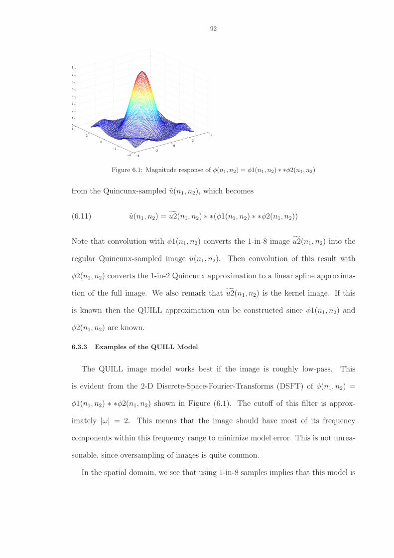
92

−4

−2

0

2

4

−4

−2

0

2

40

1

2

3

4

5

6

7

8

Figure 6.1: Magnitude response of φ(n1, n2) = φ1(n1, n2) ∗ ∗φ2(n1, n2)

from the Quincunx-sampled u(n1, n2), which becomes

(6.11) u(n1, n2) = u2(n1, n2) ∗ ∗(φ1(n1, n2) ∗ ∗φ2(n1, n2))

Note that convolution with φ1(n1, n2) converts the 1-in-8 image u2(n1, n2) into the

regular Quincunx-sampled image u(n1, n2). Then convolution of this result with

φ2(n1, n2) converts the 1-in-2 Quincunx approximation to a linear spline approxima-

tion of the full image. We also remark that u2(n1, n2) is the kernel image. If this

is known then the QUILL approximation can be constructed since φ1(n1, n2) and

φ2(n1, n2) are known.

6.3.3 Examples of the QUILL Model

The QUILL image model works best if the image is roughly low-pass. This

is evident from the 2-D Discrete-Space-Fourier-Transforms (DSFT) of φ(n1, n2) =

φ1(n1, n2) ∗ ∗φ2(n1, n2) shown in Figure (6.1). The cutoff of this filter is approx-

imately |ω| = 2. This means that the image should have most of its frequency

components within this frequency range to minimize model error. This is not unrea-

sonable, since oversampling of images is quite common.

In the spatial domain, we see that using 1-in-8 samples implies that this model is

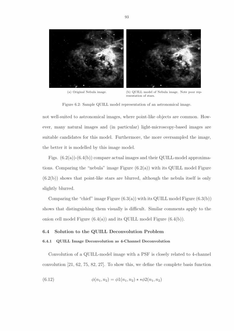
93

(a) Original Nebula image. (b) QUILL model of Nebula image. Note poor rep-resentation of stars.

Figure 6.2: Sample QUILL model representation of an astronomical image.

not well-suited to astronomical images, where point-like objects are common. How-

ever, many natural images and (in particular) light-microscopy-based images are

suitable candidates for this model. Furthermore, the more oversampled the image,

the better it is modelled by this image model.

Figs. (6.2(a))-(6.4(b)) compare actual images and their QUILL-model approxima-

tions. Comparing the “nebula” image Figure (6.2(a)) with its QUILL model Figure

(6.2(b)) shows that point-like stars are blurred, although the nebula itself is only

slightly blurred.

Comparing the “chief” image Figure (6.3(a)) with its QUILL model Figure (6.3(b))

shows that distinguishing them visually is difficult. Similar comments apply to the

onion cell model Figure (6.4(a)) and its QUILL model Figure (6.4(b)).

6.4 Solution to the QUILL Deconvolution Problem

6.4.1 QUILL Image Deconvolution as 4-Channel Deconvolution

Convolution of a QUILL-model image with a PSF is closely related to 4-channel

convolution [21, 62, 75, 82, 27]. To show this, we define the complete basis function

(6.12) φ(n1, n2) = φ1(n1, n2) ∗ ∗φ2(n1, n2)

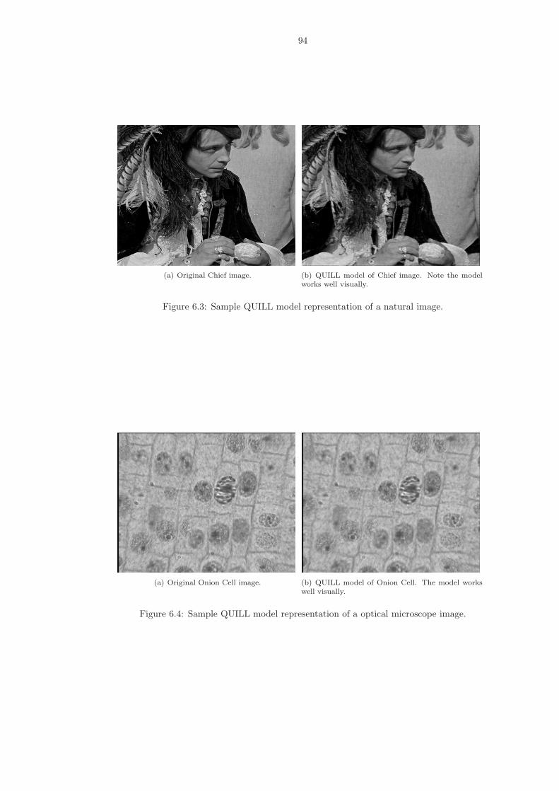
94

(a) Original Chief image. (b) QUILL model of Chief image. Note the modelworks well visually.

Figure 6.3: Sample QUILL model representation of a natural image.

(a) Original Onion Cell image. (b) QUILL model of Onion Cell. The model workswell visually.

Figure 6.4: Sample QUILL model representation of a optical microscope image.

95

and the revised PSF

(6.13) h(n1, n2) = h(n1, n2) ∗ ∗φ(n1, n2)

The 2-D blind deconvolution problem for the QUILL image model can be restated

as follows. Omitting the noise term (only for the moment) for clarity, the original

problem becomes

y(n1, n2) = h(n1, n2) ∗ ∗u(n1, n2)(6.14)

= h(n1, n2) ∗ ∗(φ(n1, n2) ∗ ∗u2(n1, n2))

= h(n1, n2) ∗ ∗u2(n1, n2)

If we now define the polyphase components

y1(n1, n2) = y(2n1, 2n2)(6.15)

y2(n1, n2) = y(2n1 + 1, 2n2)

y3(n1, n2) = y(2n1, 2n2 + 1)

y4(n1, n2) = y(2n1 + 1, 2n2 + 1)

h1(n1, n2) = h(2n1, 2n2)

h2(n1, n2) = h(2n1 + 1, 2n2)

h3(n1, n2) = h(2n1, 2n2 + 1)

h4(n1, n2) = h(2n1 + 1, 2n2 + 1)

then we have the following relationships

y1(n1, n2) = h1(n1, n2) ∗ ∗u(n1, n2)(6.16)

y2(n1, n2) = h2(n1, n2) ∗ ∗u(n1, n2)

y3(n1, n2) = h3(n1, n2) ∗ ∗u(n1, n2)

y4(n1, n2) = h4(n1, n2) ∗ ∗u(n1, n2)

96

since the 1-in-8 sampled u2(n1, n2) is effectively convolved with four different PSFs

hk(n1, n2), each of which is a (2 × 2) downsampled version of h(n1, n2).

This is evidently a four-channel SIMO (Single Input Multiple Output) system,

where u(n1, n2) is the input and each of the hk(n1, n2) represents the PSF in a given

channel.

6.4.2 2-D Bezout’s Lemma

Let hk(n1, n2), k=1,2,3,4 be four linearly independent (L×L) 2-D functions. Then

there exists, almost surely, four (L-1)×(L-1) 2-D functions gk(n1, n2), k=1,2,3,4 such

that

(6.17)4∑

k=1

hk(n1, n2) ∗ ∗gk(n1, n2) = δ(n1, n2)

This lemma has been proved for the general multichannel case in [21]. We shall

only outline the proof here so as to provide continuity. We use lexicographic ordering

to define the following matrices and vectors. Let

(6.18) h(n1, n2) = [h1(n1, n2) . . . h4(n1, n2)]′

For l1 ∈ [1, L], define the (L2 × 4L) matrix with (4X1) all-zero vectors 0 such that

(6.19) Hl1.=

h′(l1, 0) 0′ . . . 0′

h′(l1, 1) h′(l1, 0) . . . 0′

......

......

h′(l1, L) h′(l1, L − 1) . . . h′(l1, 1)

0′ h′(l1, L) . . . h′(l1, 2)

...... · · · ...

0′ 0′ . . . h′(l1, L)

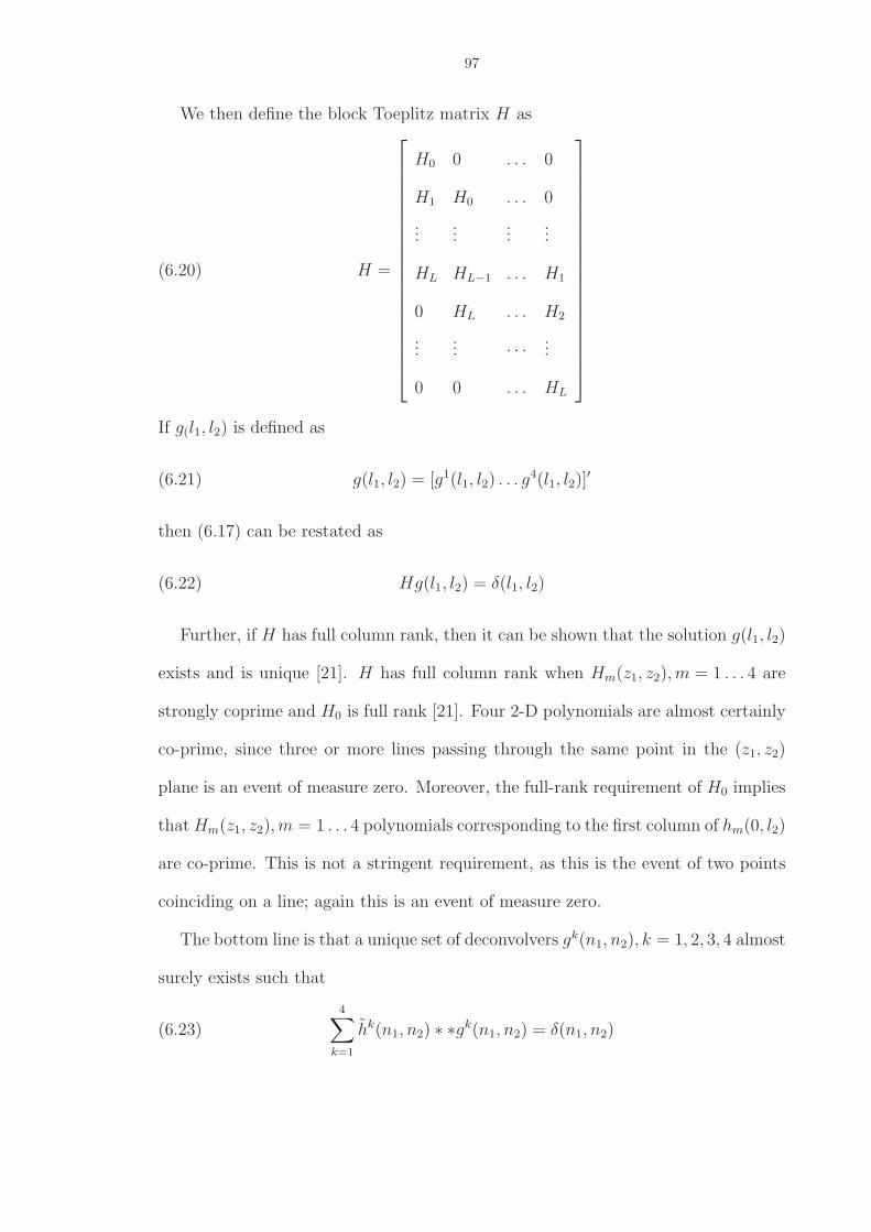
97

We then define the block Toeplitz matrix H as

(6.20) H =

H0 0 . . . 0

H1 H0 . . . 0

......

......

HL HL−1 . . . H1

0 HL . . . H2

...... · · · ...

0 0 . . . HL

If g(l1, l2) is defined as

(6.21) g(l1, l2) = [g1(l1, l2) . . . g4(l1, l2)]′

then (6.17) can be restated as

(6.22) Hg(l1, l2) = δ(l1, l2)

Further, if H has full column rank, then it can be shown that the solution g(l1, l2)

exists and is unique [21]. H has full column rank when Hm(z1, z2),m = 1 . . . 4 are

strongly coprime and H0 is full rank [21]. Four 2-D polynomials are almost certainly

co-prime, since three or more lines passing through the same point in the (z1, z2)

plane is an event of measure zero. Moreover, the full-rank requirement of H0 implies

that Hm(z1, z2),m = 1 . . . 4 polynomials corresponding to the first column of hm(0, l2)

are co-prime. This is not a stringent requirement, as this is the event of two points

coinciding on a line; again this is an event of measure zero.

The bottom line is that a unique set of deconvolvers gk(n1, n2), k = 1, 2, 3, 4 almost

surely exists such that

(6.23)4∑

k=1

hk(n1, n2) ∗ ∗gk(n1, n2) = δ(n1, n2)

98

where we are now using hk(n1, n2) constructed by (2× 2) downsampling h(n1, n2) =

h(n1, n2) ∗ ∗φ(n1, n2).

It may seem as though φ(n1, n2) is a common factor of the hk(n1, n2). But this

is not the case, since the hk(n1, n2) are downsampled from h(n1, n2). A problem will

arise only if φ(n1, n2) is an ideal low-pass filter; Figure (6.1) shows clearly that this

is not the case.

In fact, if φ(n1, n2) is an ideal low-pass filter, another problem will arise with the

QUILL model u(n1, n2) of the image u(n1, n2). The QUILL model has an implicit

spectral redundancy, since the upsampling or expanding (inserting zeros) makes the

high frequency part of the spectrum identical to the low frequency part of the spec-

trum. The spectrum of the QUILL image model does not show this explicitly, due to

convolution with φ(n1, n2), but it is still there implicitly. If φ(n1, n2) were an ideal

low-pass filter, this redundancy would be destroyed, and multichannel deconvolution

would no longer be possible.

This is implicit in the use of basis functions to parametrize the image–some in-

formation is lost. Here, this manifests itself as high frequencies being related to low

frequencies, which of course is not true in practice. This is the high-frequency error

in using the model.

6.4.3 Overall Approach

Using the 2-D Bezout Lemma, we can solve the blind deconvolution problem as

follows:

99

Convolving each of (6.16) with the corresponding gk(n1, n2) and summing yields

4∑

k=1

yk(n1, n2) ∗ ∗gk(n1, n2) =(6.24)

4∑

k=1

hk(n1, n2) ∗ ∗gk(n1, n2) ∗ ∗u(n1, n2) =

u(n1, n2) ∗ ∗4∑

k=1

hk(n1, n2) ∗ ∗gk(n1, n2)

using the distributive property of convolution. Then (6.23) yields

(6.25)4∑

k=1

yk(n1, n2) ∗ ∗gk(n1, n2) = u(n1, n2)

which is a linear system of equations in the unknowns gk(n1, n2) and u(n1, n2). Note

that half of the u(n1, n2) values are zero, since 7/8 of the u2(n1, n2) values are zero;

this is the reason for using the QUILL-type upsampling in the first place, so that the

known zero values of u(n1, n2) could be used to determine the gk(n1, n2).

Once we know u(n1, n2), we compute u(n1, n2) using (6.10). This is the recon-

structed image, which is in the form of a QUILL model.

6.4.4 Implementation of QUILL on Real Data

We have just shown how to obtain u(n1, n2) from y(n1, n2). Practically, the algo-

rithm can be broken down as follows:

1. Obtain yk(n1, n2), 1 ≤ k ≤ 4 using (6.15);

2. Form four Toeplitz-Block-Toeplitz (TBT) matrices Y1, Y2, Y3, Y4 from each of

the yk(n1, n2);

3. Concatenate the TBT matrices to form the matrix Y = [Y1|Y2|Y3|Y4]. Then

Y ~g = ~u where:

4. ~g is the stack of the four lexicographically-unwrapped deconvolvers gk(n1, n2);

100

5. ~u is the lexicographically-unwrapped Quincunx image u(n1, n2);

6. Half of the rows of Y ~g = ~u become Y1~g = ~0, since half of the values of u(n1, n2)

are zero. These can be used to determine ~g;

7. Here Y1 is the matrix consisting of half of the rows of Y ; Y2 is the matrix

containing the remaining rows of Y ;

8. Y2~g = ~u computes u(n1, n2) directly from gk(n1, n2). No deconvolution of

hk(n1, n2) from data is needed.

In fact, these two steps can be combined into the single step

(6.26)

Y1 0

Y2 −I

~g

~u

=

0

0

so that the computation consists of computing the null vector of a single matrix,

followed by convolutions with the four deconvolvers gk(n1, n2).

6.4.5 Implementation Issues

Several regularization techniques were tried. We discovered that Truncated Sin-

gular Value Decomposition [63] worked best on this problem. The reason for this is

not clear, but use of regularization techniques in inverse problems is known to be

very problem-dependent.

Another issue is selecting the size L of the PSF. Choosing L too small produced

ringing artifacts in the image. Choosing L too large produced a nullspace of dimen-

sion greater than one. This is not surprising, since translational ambiguity is now

present; the actual PSF can “rattle around” inside its assumed (L × L) support.

This too-low rank could be used as a criterion for choosing L: Choose L so that the

dimension of the null space is one. In practice, the singular values could be thresh-

olded, so that the smallest is much smaller than the next-smallest. Long tails in the

101

PSF have a minor effect on the data, which already has some modelling error since

the actual image is not modelled perfectly by a QUILL model.

6.4.6 Stochastic Formulation

Until now, we have neglected the additive noise term n(n1, n2) in the original

problem statement. Recalling that n(n1, n2) is a zero-mean white Gaussian noise

random field, the effect of the noise will be to render Y1~g = 0 unsolvable. After

adding noise to the data, matrix Y1 has full rank.

It is easy to show that the log-likelihood function for computing the maximum-

likelihood estimates ~g and ~u from the data y(n1, n2) requires that the minimun

least-squares perturbation of the data y(n1, n2) that makes the matrix in (6.26) drop

rank by one.

This suggests the use of a total-least-squares approach to find this minimum data

perturbation. However, there are other considerations, including stabilization of the

reconstructed image. That is, the problem must be regularized, so that further

perturbation of the data does not radically change the reconstructed image. This is

discussed above.

We hypothesize that the modelling error in approximating an actual image with

the QUILL model can itself be approximated with a zero-mean white Gaussian noise

random field. This is because the modelling error tends to be highpass which after

2-D convolution with a generally low-pass PSF (such as a Gaussian PSF) tends to

be roughly equalized to a flat spectrum error. This is not an important point as we

do not employ any explicit stochastic model.

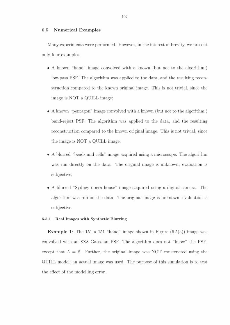
102

6.5 Numerical Examples

Many experiments were performed. However, in the interest of brevity, we present

only four examples.

• A known “hand” image convolved with a known (but not to the algorithm!)

low-pass PSF. The algorithm was applied to the data, and the resulting recon-

struction compared to the known original image. This is not trivial, since the

image is NOT a QUILL image;

• A known “pentagon” image convolved with a known (but not to the algorithm!)

band-reject PSF. The algorithm was applied to the data, and the resulting

reconstruction compared to the known original image. This is not trivial, since

the image is NOT a QUILL image;

• A blurred “beads and cells” image acquired using a microscope. The algorithm

was run directly on the data. The original image is unknown; evaluation is

subjective;

• A blurred “Sydney opera house” image acquired using a digital camera. The

algorithm was run on the data. The original image is unknown; evaluation is

subjective.

6.5.1 Real Images with Synthetic Blurring

Example 1: The 151 × 151 “hand” image shown in Figure (6.5(a)) image was

convolved with an 8X8 Gaussian PSF. The algorithm does not “know” the PSF,

except that L = 8. Further, the original image was NOT constructed using the

QUILL model; an actual image was used. The purpose of this simulation is to test

the effect of the modelling error.

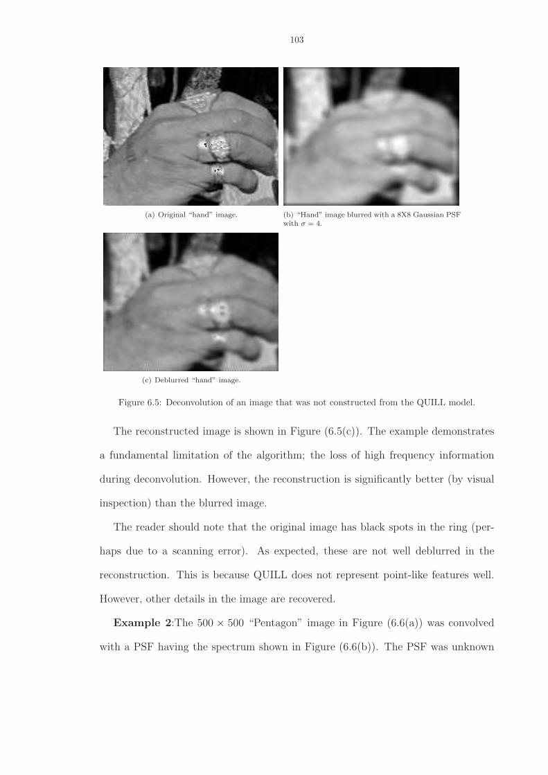
103

(a) Original “hand” image. (b) “Hand” image blurred with a 8X8 Gaussian PSFwith σ = 4.

(c) Deblurred “hand” image.

Figure 6.5: Deconvolution of an image that was not constructed from the QUILL model.

The reconstructed image is shown in Figure (6.5(c)). The example demonstrates

a fundamental limitation of the algorithm; the loss of high frequency information

during deconvolution. However, the reconstruction is significantly better (by visual

inspection) than the blurred image.

The reader should note that the original image has black spots in the ring (per-

haps due to a scanning error). As expected, these are not well deblurred in the

reconstruction. This is because QUILL does not represent point-like features well.

However, other details in the image are recovered.

Example 2:The 500 × 500 “Pentagon” image in Figure (6.6(a)) was convolved

with a PSF having the spectrum shown in Figure (6.6(b)). The PSF was unknown

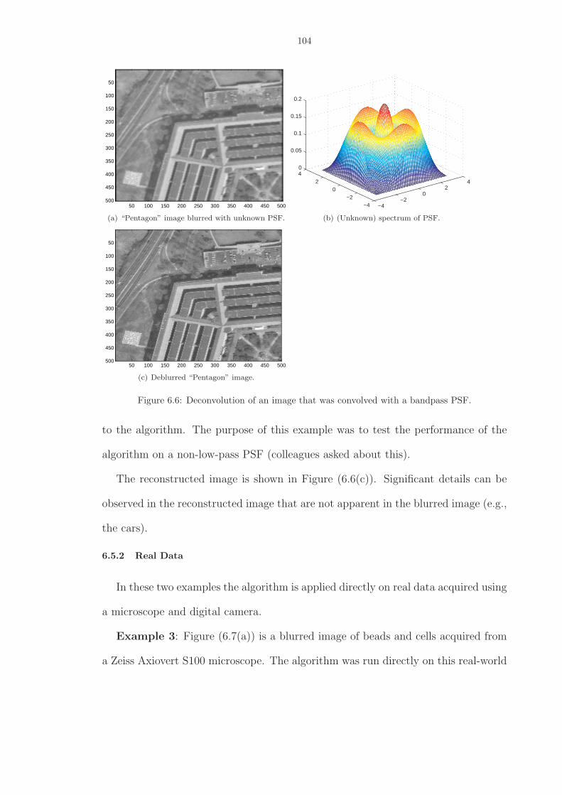
104

50 100 150 200 250 300 350 400 450 500

50

100

150

200

250

300

350

400

450

500

(a) “Pentagon” image blurred with unknown PSF.

−4−2

02

4

−4−2

02

40

0.05

0.1

0.15

0.2

(b) (Unknown) spectrum of PSF.

50 100 150 200 250 300 350 400 450 500

50

100

150

200

250

300

350

400

450

500

(c) Deblurred “Pentagon” image.

Figure 6.6: Deconvolution of an image that was convolved with a bandpass PSF.

to the algorithm. The purpose of this example was to test the performance of the

algorithm on a non-low-pass PSF (colleagues asked about this).

The reconstructed image is shown in Figure (6.6(c)). Significant details can be

observed in the reconstructed image that are not apparent in the blurred image (e.g.,

the cars).

6.5.2 Real Data

In these two examples the algorithm is applied directly on real data acquired using

a microscope and digital camera.

Example 3: Figure (6.7(a)) is a blurred image of beads and cells acquired from

a Zeiss Axiovert S100 microscope. The algorithm was run directly on this real-world

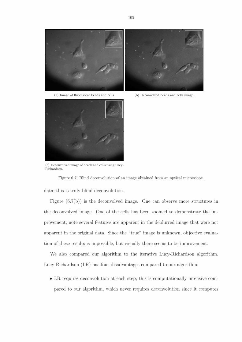
105

(a) Image of fluorescent beads and cells. (b) Deconvolved beads and cells image.

(c) Deconvolved image of beads and cells using Lucy-Richardson.

Figure 6.7: Blind deconvolution of an image obtained from an optical microscope.

data; this is truly blind deconvolution.

Figure (6.7(b)) is the deconvolved image. One can observe more structures in

the deconvolved image. One of the cells has been zoomed to demonstrate the im-

provement; note several features are apparent in the deblurred image that were not

apparent in the original data. Since the “true” image is unknown, objective evalua-

tion of these results is impossible, but visually there seems to be improvement.

We also compared our algorithm to the iterative Lucy-Richardson algorithm.

Lucy-Richardson (LR) has four disadvantages compared to our algorithm:

• LR requires deconvolution at each step; this is computationally intensive com-

pared to our algorithm, which never requires deconvolution since it computes

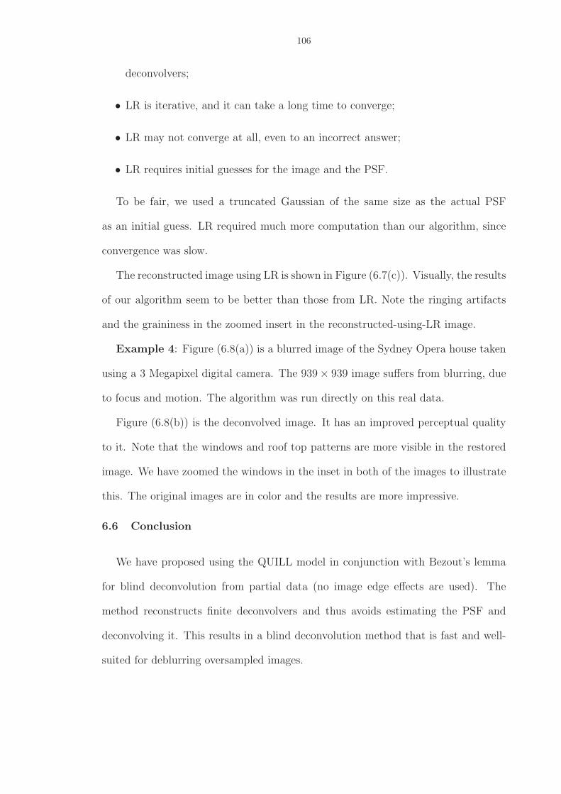
106

deconvolvers;

• LR is iterative, and it can take a long time to converge;

• LR may not converge at all, even to an incorrect answer;

• LR requires initial guesses for the image and the PSF.

To be fair, we used a truncated Gaussian of the same size as the actual PSF

as an initial guess. LR required much more computation than our algorithm, since

convergence was slow.

The reconstructed image using LR is shown in Figure (6.7(c)). Visually, the results

of our algorithm seem to be better than those from LR. Note the ringing artifacts

and the graininess in the zoomed insert in the reconstructed-using-LR image.

Example 4: Figure (6.8(a)) is a blurred image of the Sydney Opera house taken

using a 3 Megapixel digital camera. The 939 × 939 image suffers from blurring, due

to focus and motion. The algorithm was run directly on this real data.

Figure (6.8(b)) is the deconvolved image. It has an improved perceptual quality

to it. Note that the windows and roof top patterns are more visible in the restored

image. We have zoomed the windows in the inset in both of the images to illustrate

this. The original images are in color and the results are more impressive.

6.6 Conclusion

We have proposed using the QUILL model in conjunction with Bezout’s lemma

for blind deconvolution from partial data (no image edge effects are used). The

method reconstructs finite deconvolvers and thus avoids estimating the PSF and

deconvolving it. This results in a blind deconvolution method that is fast and well-

suited for deblurring oversampled images.

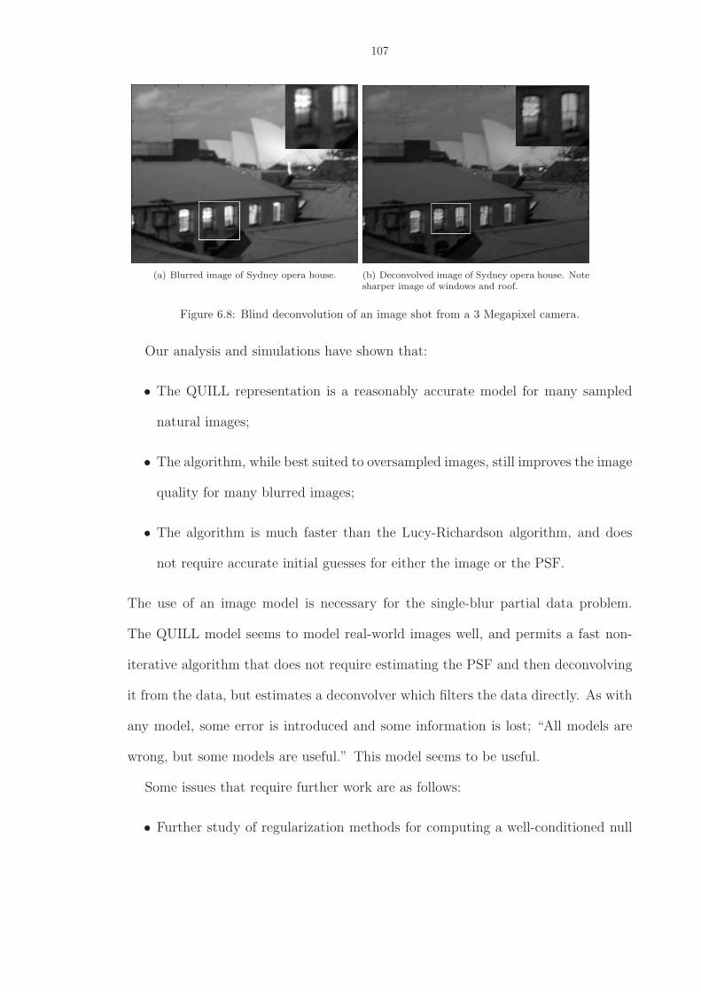
107

(a) Blurred image of Sydney opera house. (b) Deconvolved image of Sydney opera house. Notesharper image of windows and roof.

Figure 6.8: Blind deconvolution of an image shot from a 3 Megapixel camera.

Our analysis and simulations have shown that:

• The QUILL representation is a reasonably accurate model for many sampled

natural images;

• The algorithm, while best suited to oversampled images, still improves the image

quality for many blurred images;

• The algorithm is much faster than the Lucy-Richardson algorithm, and does

not require accurate initial guesses for either the image or the PSF.

The use of an image model is necessary for the single-blur partial data problem.

The QUILL model seems to model real-world images well, and permits a fast non-

iterative algorithm that does not require estimating the PSF and then deconvolving

it from the data, but estimates a deconvolver which filters the data directly. As with

any model, some error is introduced and some information is lost; “All models are

wrong, but some models are useful.” This model seems to be useful.

Some issues that require further work are as follows:

• Further study of regularization methods for computing a well-conditioned null

108

vector from the data matrix. This means that the null vector (which includes

u(n1, n2)) is not sensitive to data perturbations;

• Development of algorithms for perturbing data to create a 1-D null space for

the specific case of Poisson noise;

• Further study of proper choice of the PSF size L. Although this does not seem

to be a major issue in practice, it would be nice to have a model-order-selection-

type stochastic procedure.

CHAPTER VII

Contrast Transfer Function estimation for cryo and

cryo-tomo electron microscopy images

7.1 Introduction

Cryo-electron microscopy (EM) is an important tool for visualizing the structure of

molecular assemblies and sub-cellular structure allowing delicate biological samples

to be preserved in their native states. Unfortunately, cryo samples are extremely

sensitive to radiation damage and thus must be imaged at very low electron doses,

resulting in low contrast images having poor signal to noise ratios. This problem is

exacerbated in cryo-EM tomography, where the maximum allowable dose must be

spread over the 100-200 tilted images usually recorded from a single specimen.

Since thin biological samples are weak phase objects, contrast is generated via

a combination of spherical aberration and defocusing. Unfortunately, this intro-

duces significant distortions in the image [67], which along with other factors such as

specimen drift and the non-ideal response characteristics of the detection media ulti-

mately limit the maximum useful resolution of the electron micrograph. Accurately

correcting image aberrations is important to maximize the obtainable resolution

[57, 34, 52, 64]. For thin biological specimens, the characteristic response of the EM

system is expressed by the contrast transfer function (CTF), which describes the

fidelity with which spatial information is transferred from input to output across a

109

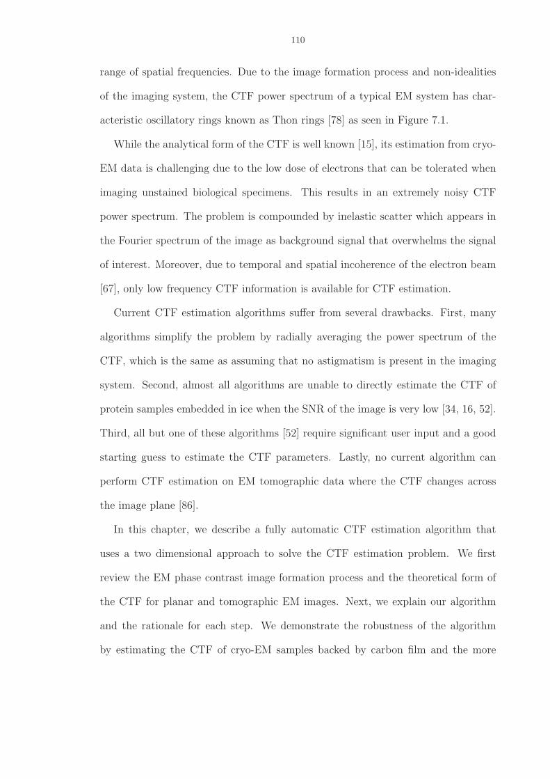
110

range of spatial frequencies. Due to the image formation process and non-idealities

of the imaging system, the CTF power spectrum of a typical EM system has char-

acteristic oscillatory rings known as Thon rings [78] as seen in Figure 7.1.

While the analytical form of the CTF is well known [15], its estimation from cryo-

EM data is challenging due to the low dose of electrons that can be tolerated when

imaging unstained biological specimens. This results in an extremely noisy CTF

power spectrum. The problem is compounded by inelastic scatter which appears in

the Fourier spectrum of the image as background signal that overwhelms the signal

of interest. Moreover, due to temporal and spatial incoherence of the electron beam

[67], only low frequency CTF information is available for CTF estimation.

Current CTF estimation algorithms suffer from several drawbacks. First, many

algorithms simplify the problem by radially averaging the power spectrum of the

CTF, which is the same as assuming that no astigmatism is present in the imaging

system. Second, almost all algorithms are unable to directly estimate the CTF of

protein samples embedded in ice when the SNR of the image is very low [34, 16, 52].

Third, all but one of these algorithms [52] require significant user input and a good

starting guess to estimate the CTF parameters. Lastly, no current algorithm can

perform CTF estimation on EM tomographic data where the CTF changes across

the image plane [86].

In this chapter, we describe a fully automatic CTF estimation algorithm that

uses a two dimensional approach to solve the CTF estimation problem. We first

review the EM phase contrast image formation process and the theoretical form of

the CTF for planar and tomographic EM images. Next, we explain our algorithm

and the rationale for each step. We demonstrate the robustness of the algorithm

by estimating the CTF of cryo-EM samples backed by carbon film and the more

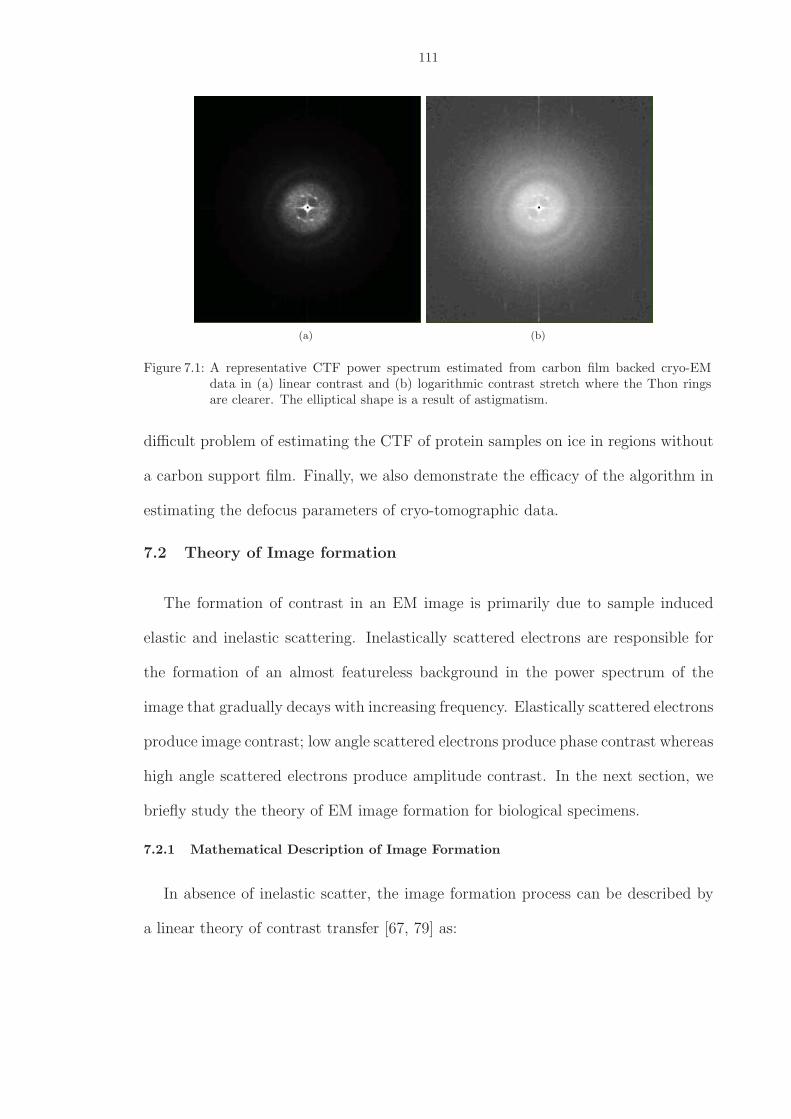
111

(a) (b)

Figure 7.1: A representative CTF power spectrum estimated from carbon film backed cryo-EMdata in (a) linear contrast and (b) logarithmic contrast stretch where the Thon ringsare clearer. The elliptical shape is a result of astigmatism.

difficult problem of estimating the CTF of protein samples on ice in regions without

a carbon support film. Finally, we also demonstrate the efficacy of the algorithm in

estimating the defocus parameters of cryo-tomographic data.

7.2 Theory of Image formation

The formation of contrast in an EM image is primarily due to sample induced

elastic and inelastic scattering. Inelastically scattered electrons are responsible for

the formation of an almost featureless background in the power spectrum of the

image that gradually decays with increasing frequency. Elastically scattered electrons

produce image contrast; low angle scattered electrons produce phase contrast whereas

high angle scattered electrons produce amplitude contrast. In the next section, we

briefly study the theory of EM image formation for biological specimens.

7.2.1 Mathematical Description of Image Formation

In absence of inelastic scatter, the image formation process can be described by

a linear theory of contrast transfer [67, 79] as:

112

(7.1) i(r, θ) = h(r, θ) ⊗ o(r, θ) ⊗ e(r, θ) + n

where i,h and o are the image, transfer function of the system and object re-

spectively and r, θ are polar co-ordinates. The ⊗ operator describes the convolution

operation. The envelope function e(r, θ) describes the reduction in image contrast

with increasing spatial frequency due to the coherence of the electron beam, lens cur-

rent instability, stage drift and modulation transfer function (MTF) of the recording

media [67]. We assume the noise in the system, n, is a combination of Poisson noise

due to photodetection and Gaussian noise, e.g., due to detector or scanner electron-

ics. We approximate both by using a mixed Gaussian noise model as described in

[46, 31].

Applying the Fourier transform to (7.1):

(7.2) I(q, φ) = CTF (q, φ)O(q, φ)E(q, φ) + N

where q is the spatial frequency, φ is the angle ordinate and CTF (q, φ) is the Fourier

transform of h(r, θ) or contrast transfer function (CTF) of the system.

In biological samples, inelastic scattering contributes significantly to the image

formation process [58]. This is seen in the power spectrum of the image as an additive

low frequency background, S(q, φ):

(7.3) I2(q, φ) = S(q, φ) + CTF 2(q, φ)O2(q, φ)E2(q, φ) + N2

7.3 CTF Formula

7.3.1 Planar EM

For thin biological specimens assuming a weak amplitude-weak phase approxima-

tion [67, 58, 84], the theoretical form of the CTF can be expressed as:

113

(7.4) CTF (q, φ) =√

1 − α2 sin χ(q, φ) − α cos χ(q, φ)

where α is an amplitude contrast factor ( 0 ≤ α ≤ 1) and χ(q, φ) is the scattering

angle dependent path length difference of the wavefront of the electron beam [67]. χ

can be expressed as:

(7.5) χ(q, φ) = π/2{Csλ3q4 − λq2(2∆fmean + ∆fdiffcos(2φ − 2φA))}

where Cs is the spherical aberration of the objective lens, ∆fmean is a mean defocus

parameter, ∆fdiff and φA are parameters describing the astigmatism of the CTF and

λ is the wavelength of the electron beam.

7.3.2 Tomographic EM

In EM tomography, images are formed as projections of a sample tilted incre-

mentally with respect to a horizontal plane. The mean defocus is no longer uniform

across the sample plane but is dependent on the point of measurement and the tilt

angle. Apart from this difference, the theoretical form of the tomographic CTF is

identical to (7.4). As shown in the Appendix, for a specimen rotated by an angle

θtilt and whose the rotation axis makes an angle θrot with respect to the y axis, the

mean defocus, ∆fmean is related to θtilt and θrot at a point U(x, y, z) on the sample

plane by the equation

(7.6) ∆fmean = (x cos θrot + y sin θrot) tan θtilt + ∆fo

where x cos θrot + y sin θrot is the projection of the distance between U(x, y, z) on

the sample plane and the rotation axis on the zero-tilt plane.

114

The tilt angle can be estimated by measuring the mean defocus at any two points

on the sample plane. If the mean defoci for two points (x1, y1, z1) and (x2, y2, z2)

on the sample plane are ∆fx1,y1,z1and ∆fx2,y2,z2

respectively , the tilt angle θtilt

can be determined as θtilt = tan−1((∆fx1,y1,z1− ∆fx2,y2,z2

)/((x1 − x2) cos θrot + (y1 −

y2) sin θrot)).

7.4 Algorithm for CTF Estimation

A description of the CTF requires knowledge of the parameters described in (7.4).

Of these, the spherical aberration term Cs is provided by the microscope manufac-

turer and the wavelength λ is a known function of accelerating voltage [67]. That

leaves the terms ∆fmean, ∆fdiff , φA and the amplitude contrast factor, α to be

determined.

Our CTF estimation algorithm first approximates the CTF power spectrum us-

ing an approach similar to periodogram averaging [16]. A residual power spectrum

I2res(q, φ) is computed by estimating and subtracting the background term S(q) from

the CTF power spectrum. The lowest and the highest frequencies are then masked

in I2res(q, φ) in which the power spectrum of the object (also known as ”structure

factor”) and noise respectively dominate. Finally, the algorithm estimates the CTF

parameters from the residual power spectrum using a combination of coarse grid

search and a constrained conjugate gradients (CCG) scheme. The one parameter

that does need to be estimated by the user is the amount of amplitude contrast, α.

7.4.1 Obtaining the Power Spectrum of the CTF

In cryo-EM, the CTF power spectrum is usually approximated by calculating the

power spectrum of a small blank region where there is a carbon support film. As

seen in (7.3), the power spectrum of the image I2(q, φ), contains a strong noise term,

115

N2, that dominates the CTF power spectrum.

To supress noise, an average power spectrum was calculated over 50 random ar-

eas of the micrograph similar to periodogram averaging [16]. Averaging over random

areas also helps to suppress the contributions from specimen structure when deter-

mining the CTF over the sample region. The success of this scheme depends on one

of the following assumptions: (1) only a few sampling areas contain the specimen so

that the contribution of the sample structure factor in the estimate is small, or (2)

the structure factor over the random areas is sufficiently incoherent to be averaged

out. In practice, we have found these assumptions to be quite valid. The power

spectrum equation (7.3), averaged over these random image samples can then be

written as:

(7.7) 〈I2(q, φ)〉 = S(q, φ) + c1CTF 2(q, φ)E2(q, φ) + k

where c1 and k are constants. We will refer to this mean power spectrum as the

CTF power spectrum. Representative CTF power spectra obtained under 4 common

imaging conditions are shown in Figure 7.2.

7.4.2 Background Fitting and Subtraction

Since the background S(q, φ) dominates the CTF power spectrum 〈I2(q, φ)〉, its

removal makes the parameter estimation step more reliable. While the background

power spectrum is a two-dimensional function, its estimation in a 2D parametric

form is problematic due to the low signal to noise ratio (SNR) of cryo-EM images. It

is important to note that because of sample structure, drift, tilt, etc., the anisotropy

in the background need not match the anisotropy in the CTF caused by astigma-

tism. Thus it is important to independently determine the radial asymmetry of the

116

(a) (b)

(c) (d)

Figure 7.2: Examples of averaged CTF power spectra in logarithmic scale, obtained after samplingat 50 random points in the micrograph. Figure 7.2(a) is a representative CTF obtainedfrom a negative stained image. Due to the high SNR, Thon rings are clearly visibile.Figure 7.2(b) is the CTF power spectrum obtained from a cryo sample with carbonsupport film. Despite a lower SNR the first three Thon rings are still visible. Figure7.2(c) depicts a CTF power spectrum obtained from a sample of bacteria flagella fila-ment in ice. Due to the absence of carbon support film the CTF is barely visible. TheFourier transform of the specimen is also observed as lines in the power spectrum.[91]Figure 7.2(d) shows a representative power spectrum from a cryo-EM tomograph. Dueto the very low electron dose, the SNR of the CTF power spectrum is very low and theThon rings are barely seen.

117

background. As a compromise between SNR and accounting for these effects, we

estimate the background by dividing 〈I2(q, φ)〉 into 8 sectors and fitting a quartic

polynomial to the sector averages.

The resultant background S(q, φ) is subtracted from 〈I2(q, φ)〉 to form a residual

power spectrum, P (q, φ).

(7.8) P (q, φ) = 〈I2(q, φ)〉 − S(q, φ) = c1CTF 2(q, φ)E2(q, φ) + k

7.4.3 Masking

The CTF power spectrum is dominated by the sample structure factor at low fre-

quencies and by noise at high frequencies. Masking out frequencies at these extremes

from the residual power spectrum improves the reliability of the CTF parameter es-

timation.

For the higher frequency cutoff, we use what is known as the predominant power

frequency [34]. This is defined as the frequency below which 99 percent of the

signal energy is present in the residual CTF. The lower frequency cutoff is chosen

within the first CTF ring. The location is not critical and is easily estimated from

the approximate defocus parameters obtained in the initial coarse grid search as

described in the next section. The masked CTF power spectrum, Pm(q, φ) is given

by:

(7.9) Pm(q, φ) = P (q, φ)M(q, φ)

where M(q, φ) is the mask.

7.4.4 Determination of Defocus and Astigmatism Parameters

CTF defocus parameters are estimated using I2res,m(q, φ). The parameter estima-

tion problem is solved by a cost function minimization using a robust constrained

118

conjugate gradients approach (CCG) [23]. We chose the following cross correlation

function as our cost function as it has been shown to be an effective measure in CTF

parameter estimation [57]:

(7.10) ψ = 1 − Σx,yPm ∗ CTF 2

√(Σx,yCTF 4)(Σx,yP 2

m))

Directly using the entire two dimensional data in the cost function maximizes

the use of the experimental data and minimizes the need for ad hoc pre-processing.

The non-convexity of the CTF parameter optimization surface gives rise to several

local minima many of which are eliminated by providing a good starting guess. This

step is automated in our algorithm by performing a 256 point grid search across

the optimization plane keeping the amplitude contrast parameter (α) constant. To

expedite the algorithm, we use the following optimization constraints:

0.5µm ≤ ∆fmean ≤ 15µm(7.11)

0µm ≤ ∆fdiff ≤ 6µm(7.12)

0 ≤ φA ≤ π(7.13)

These constraints which are appropriate for the CTFs observed in our datasets,

can be readily modified to suit individual needs.

In practice, the amplitude contrast parameter, α, is quite difficult to estimate

accurately, and in other programs is a user supplied parameter typically around 7%

for cryo images and 15% for negative stain [79]. In our software, this is one term

that needs to be provided by the user.

119

7.4.5 CTF estimation for Tomographic Micrographs

Cryo-EM tomography, especially when coupled with averaging, has now pro-

gressed to the point where CTF correction of tilted images is becoming useful.

Similarly, determining and correcting the CTF on tilted images could be equally

beneficial when using the Random Conical Tilt method [66]. In either case, the first

step is the accurate determination of appropriate CTF parameters across the tilted

image. Apart from astigmatism and amplitude contrast parameters, the CTF of a

tomographic image is completely described when the tilt angle and mean defocus at

a given point on the specimen plane are specified. For tomographic CTF estimation,

the planar EM algorithm was modified to account for a variable mean defocus and

tilt angle.

A schematic of the CTF estimation algorithm for tomographic EM data is shown

in Figure 7.3. The algorithm approximates the CTF power spectrum and estimates

CTF parameters in 6 areas that are parallel to the tilt axis (we refer to these areas

as stripes). The CTF parameter estimates of each stripe are assumed to correspond

to the CTF at the centroid of the stripes. The astigmatism of the CTF is assumed

to be constant over the specimen plane and independent of the tilt angle, θtilt. It is

estimated by calculating the mean ∆fdiff and φa estimates over all the stripes for the

tilted sample. From (7.6), the mean defocus estimates of each stripe (∆fmean) should

lie on a line with slope tan θtilt. The mean defocus at the rotation axis, ∆fo is given

by the y-intercept of the fitted line and tilt angle, tan θtilt by the slope. In practice,

for cryo EM images, the tilt angle estimates of the algorithm are not as accurate as

the nominal tilt angles of the microscope. As a result, the program performs two

least squares fits to improve the accuracy of the mean defocus parameter. ∆fo is

estimated as the y-intercept of a least squares fit using the tangent of the nominal

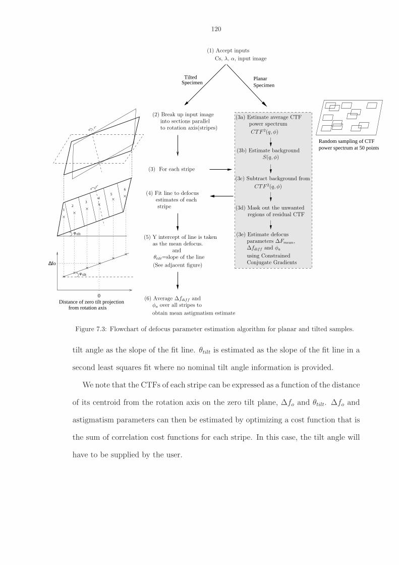
120

Random sampling of CTFpower spectrum at 50 points

φ tilt

φ tilt

Distance of zero tilt projectionfrom rotation axis

fo∆

SpecimenTilted Planar

Specimen

r’

23

45

6

1

r’

0

(2) Break up input imageinto sections parallelto rotation axis(stripes)

(4) Fit line to defocusestimates of eachstripe

(5) Y intercept of line is takenas the mean defocus.

andθtilt=slope of the line

(See adjacent figure)

(6) Average ∆fdiff and

obtain mean astigmatism estimate

power spectrum

regions of residual CTF

CTF 2(q, φ)

(3e) Estimate defocusparameters ∆Fmean,∆fdiff and φa

using ConstrainedConjugate Gradients

(3b) Estimate backgroundS(q, φ)

(3a) Estimate average CTF

(3c) Subtract background from

(3d) Mask out the unwanted

(1) Accept inputs

Cs, λ, α, input image

(3)

CTF 2(q, φ)

For each stripe

φa over all stripes to

Figure 7.3: Flowchart of defocus parameter estimation algorithm for planar and tilted samples.

tilt angle as the slope of the fit line. θtilt is estimated as the slope of the fit line in a

second least squares fit where no nominal tilt angle information is provided.

We note that the CTFs of each stripe can be expressed as a function of the distance

of its centroid from the rotation axis on the zero tilt plane, ∆fo and θtilt. ∆fo and

astigmatism parameters can then be estimated by optimizing a cost function that is

the sum of correlation cost functions for each stripe. In this case, the tilt angle will

have to be supplied by the user.

121

7.5 Results

7.5.1 Ice on Carbon Film Defocus Series Data

To evaluate the effectiveness of the algorithm in measuring defocus parameters of

cryo-EM data , the nominal defocus was compared to the estimated mean defocus,

∆fmean, over a range of defoci. Comparing the relative differences between nominal

defocus and ∆fmean is a better measure of accuracy than comparing their absolute

values due to inherent offset error in the nominal defocus [52].

The nominal defocus of the microscope was changed manually from 1.44 µm to

8 µm in increments keeping astigmatism constant. Defocus was estimated using the

algorithm for a series of micrographs imaged at a magnification of 61,000 with a

dose of 5 electrons per A2. Fig. 7.4 shows a plot of measured defocus versus nominal

defocus. The correlation coefficient of the points with the least squares fit line is

0.999 indicating that the measured defocus accuracy is quite good. The offset error

of the nominal defocus is 0.099 µm as indicated by the x-intercept of the line.

7.5.2 Validation of Determined Defocus Values

Tani [77] and Mullick [52] have developed programs that have been shown to

estimate CTFs of cryo-EM data with carbon support film quite accurately. Tani’s

program, PLTCTFX, approximates the CTF power spectrum by calculating the

power spectrum of a manually selected region of the micrograph. CTF parameters

are estimated by one dimensional parameter fitting on 5 sector averages of the CTF

power spectrum. Mullick’s program, Automatic CTF Estimation (ACE), uses a dif-

ferent approach. The first CTF ring is detected using two-dimensional edge-detection

to determine astigmatism. Defocus parameters are determined by one dimensional

fitting of the elliptically averaged CTF. A key difference between our algorithm and

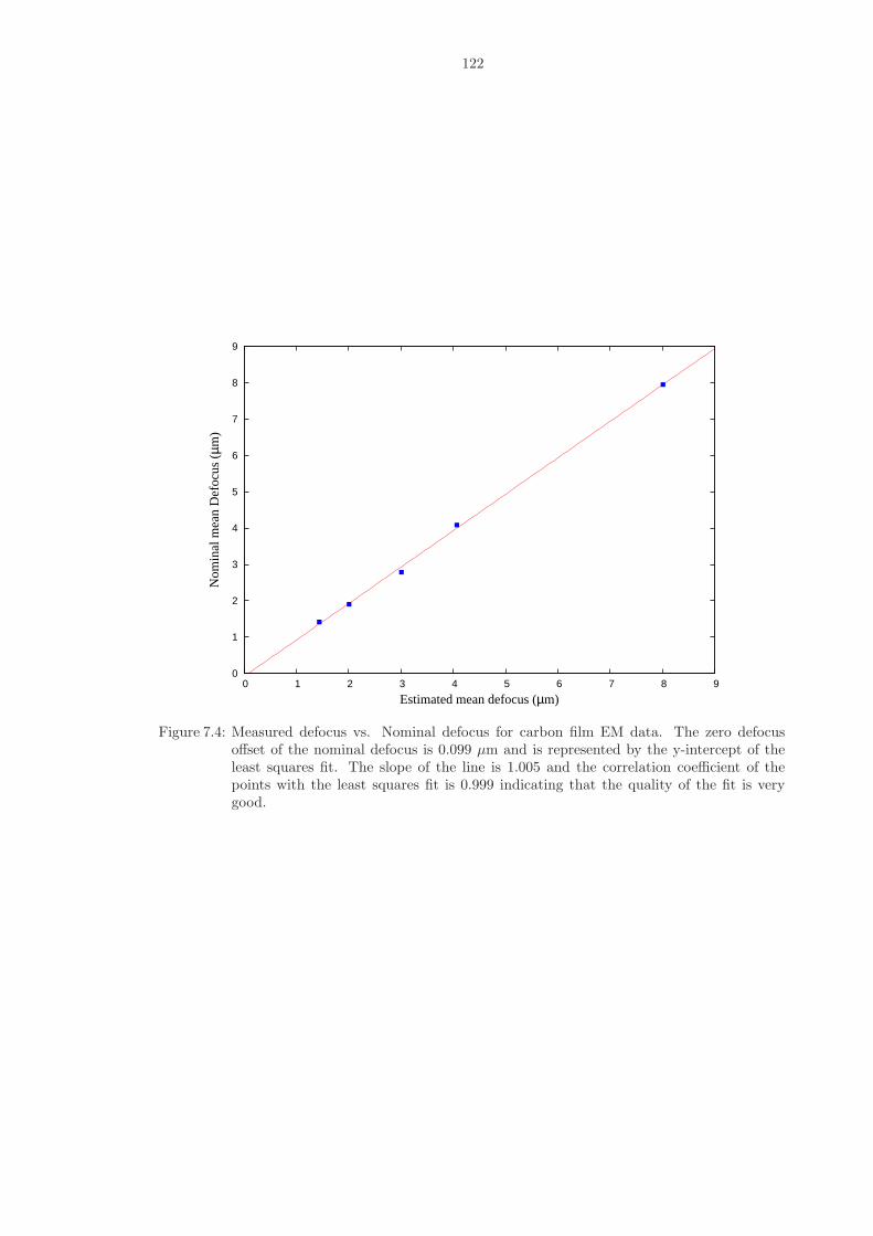
122

0

1

2

3

4

5

6

7

8

9

0 1 2 3 4 5 6 7 8 9

Nom

inal

mea

n D

efoc

us (

µm)

Estimated mean defocus (µm)

Figure 7.4: Measured defocus vs. Nominal defocus for carbon film EM data. The zero defocusoffset of the nominal defocus is 0.099 µm and is represented by the y-intercept of theleast squares fit. The slope of the line is 1.005 and the correlation coefficient of thepoints with the least squares fit is 0.999 indicating that the quality of the fit is verygood.

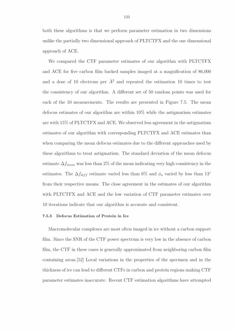
123

both these algorithms is that we perform parameter estimation in two dimensions

unlike the partially two dimensional approach of PLTCTFX and the one dimensional

approach of ACE.

We compared the CTF parameter estimates of our algorithm with PLTCTFX

and ACE for five carbon film backed samples imaged at a magnification of 86,000

and a dose of 10 electrons per A2 and repeated the estimation 10 times to test

the consistency of our algorithm. A different set of 50 random points was used for

each of the 10 measurements. The results are presented in Figure 7.5. The mean

defocus estimates of our algorithm are within 10% while the astigmatism estimates

are with 15% of PLTCTFX and ACE. We observed less agreement in the astigmatism

estimates of our algorithm with corresponding PLTCTFX and ACE estimates than

when comparing the mean defocus estimates due to the different approaches used by

these algorithms to treat astigmatism. The standard deviation of the mean defocus

estimate ∆fmean was less than 2% of the mean indicating very high consistency in the

estimates. The ∆fdiff estimate varied less than 6% and φa varied by less than 13◦

from their respective means. The close agreement in the estimates of our algorithm

with PLTCTFX and ACE and the low variation of CTF parameter estimates over

10 iterations indicate that our algorithm is accurate and consistent.

7.5.3 Defocus Estimation of Protein in Ice

Macromolecular complexes are most often imaged in ice without a carbon support

film. Since the SNR of the CTF power spectrum is very low in the absence of carbon

film, the CTF in these cases is generally approximated from neighboring carbon film

containing areas.[52] Local variations in the properties of the specimen and in the

thickness of ice can lead to different CTFs in carbon and protein regions making CTF

parameter estimates inaccurate. Recent CTF estimation algorithms have attempted

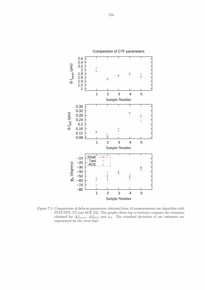
124

1 1.2 1.4 1.6 1.8

2 2.2 2.4 2.6

5 4 3 2 1

∆ f m

ean

(µm

)

Sample Number

Comparision of CTF parameters

0.36 0.32 0.28 0.24

0.2 0.16 0.12 0.08

5 4 3 2 1

∆ f

diff

(µm

)

Sample Number

−10−20−30−40−50−60−70−80

5 4 3 2 1

φ A (

degr

ees)

Sample Number

ShahTaniACE

Figure 7.5: Comparision of defocus parameters obtained from 10 measurements our algorithm withPLTCTFX [77] and ACE [52]. The graphs (from top to bottom) compare the estimatesobtained for ∆fmean, ∆fdiff and φA. The standard deviation of our estimates arerepresented by the error bars.

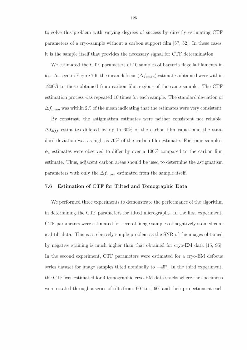
125

to solve this problem with varying degrees of success by directly estimating CTF

parameters of a cryo-sample without a carbon support film [57, 52]. In these cases,

it is the sample itself that provides the necessary signal for CTF determination.

We estimated the CTF parameters of 10 samples of bacteria flagella filaments in

ice. As seen in Figure 7.6, the mean defocus (∆fmean) estimates obtained were within

1200A to those obtained from carbon film regions of the same sample. The CTF

estimation process was repeated 10 times for each sample. The standard deviation of

∆fmean was within 2% of the mean indicating that the estimates were very consistent.

By constrast, the astigmatism estimates were neither consistent nor reliable.

∆fdiff estimates differed by up to 60% of the carbon film values and the stan-

dard deviation was as high as 70% of the carbon film estimate. For some samples,

φa estimates were observed to differ by over a 100% compared to the carbon film

estimate. Thus, adjacent carbon areas should be used to determine the astigmatism

parameters with only the ∆fmean estimated from the sample itself.

7.6 Estimation of CTF for Tilted and Tomographic Data

We performed three experiments to demonstrate the performance of the algorithm

in determining the CTF parameters for tilted micrographs. In the first experiment,

CTF parameters were estimated for several image samples of negatively stained con-

ical tilt data. This is a relatively simple problem as the SNR of the images obtained

by negative staining is much higher than that obtained for cryo-EM data [15, 95].

In the second experiment, CTF parameters were estimated for a cryo-EM defocus

series dataset for image samples tilted nominally to −45◦. In the third experiment,

the CTF was estimated for 4 tomographic cryo-EM data stacks where the specimens

were rotated through a series of tilts from -60◦ to +60◦ and their projections at each

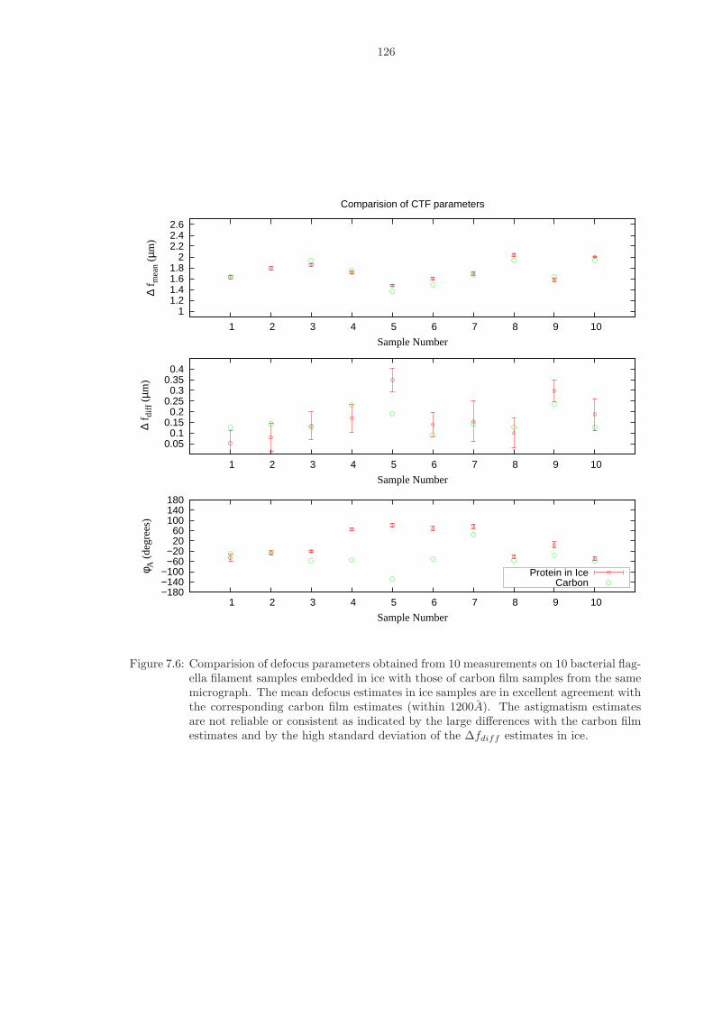
126

1 1.2 1.4 1.6 1.8

2 2.2 2.4 2.6

10 9 8 7 6 5 4 3 2 1

∆ f m

ean

(µm

)

Sample Number

Comparision of CTF parameters

0.4 0.35

0.3 0.25

0.2 0.15

0.1 0.05

10 9 8 7 6 5 4 3 2 1

∆ f

diff

(µm

)

Sample Number

180 140 100

60 20

−20−60

−100−140−180

10 9 8 7 6 5 4 3 2 1

φ A (

degr

ees)

Sample Number

Protein in IceCarbon

Figure 7.6: Comparision of defocus parameters obtained from 10 measurements on 10 bacterial flag-ella filament samples embedded in ice with those of carbon film samples from the samemicrograph. The mean defocus estimates in ice samples are in excellent agreement withthe corresponding carbon film estimates (within 1200A). The astigmatism estimatesare not reliable or consistent as indicated by the large differences with the carbon filmestimates and by the high standard deviation of the ∆fdiff estimates in ice.

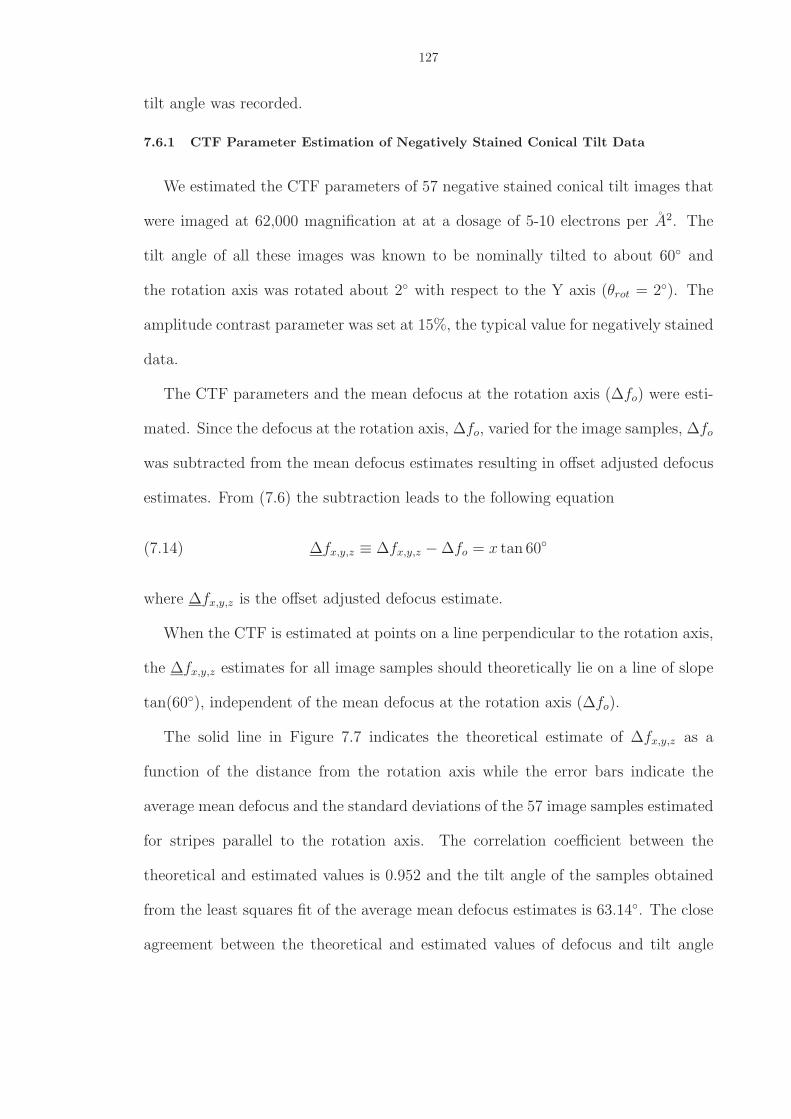
127

tilt angle was recorded.

7.6.1 CTF Parameter Estimation of Negatively Stained Conical Tilt Data

We estimated the CTF parameters of 57 negative stained conical tilt images that

were imaged at 62,000 magnification at at a dosage of 5-10 electrons per A2. The

tilt angle of all these images was known to be nominally tilted to about 60◦ and

the rotation axis was rotated about 2◦ with respect to the Y axis (θrot = 2◦). The

amplitude contrast parameter was set at 15%, the typical value for negatively stained

data.

The CTF parameters and the mean defocus at the rotation axis (∆fo) were esti-

mated. Since the defocus at the rotation axis, ∆fo, varied for the image samples, ∆fo

was subtracted from the mean defocus estimates resulting in offset adjusted defocus

estimates. From (7.6) the subtraction leads to the following equation

(7.14) ∆fx,y,z ≡ ∆fx,y,z − ∆fo = x tan 60◦

where ∆fx,y,z is the offset adjusted defocus estimate.

When the CTF is estimated at points on a line perpendicular to the rotation axis,

the ∆fx,y,z estimates for all image samples should theoretically lie on a line of slope

tan(60◦), independent of the mean defocus at the rotation axis (∆fo).

The solid line in Figure 7.7 indicates the theoretical estimate of ∆fx,y,z as a

function of the distance from the rotation axis while the error bars indicate the

average mean defocus and the standard deviations of the 57 image samples estimated

for stripes parallel to the rotation axis. The correlation coefficient between the

theoretical and estimated values is 0.952 and the tilt angle of the samples obtained

from the least squares fit of the average mean defocus estimates is 63.14◦. The close

agreement between the theoretical and estimated values of defocus and tilt angle

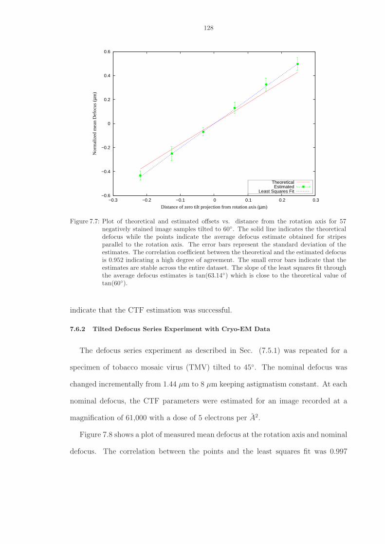
128

−0.6

−0.4

−0.2

0

0.2

0.4

0.6

−0.3 −0.2 −0.1 0 0.1 0.2 0.3

Nor

mal

ized

mea

n D

efoc

us (

µm)

Distance of zero tilt projection from rotation axis (µm)

TheoreticalEstimated

Least Squares Fit

Figure 7.7: Plot of theoretical and estimated offsets vs. distance from the rotation axis for 57negatively stained image samples tilted to 60◦. The solid line indicates the theoreticaldefocus while the points indicate the average defocus estimate obtained for stripesparallel to the rotation axis. The error bars represent the standard deviation of theestimates. The correlation coefficient between the theoretical and the estimated defocusis 0.952 indicating a high degree of agreement. The small error bars indicate that theestimates are stable across the entire dataset. The slope of the least squares fit throughthe average defocus estimates is tan(63.14◦) which is close to the theoretical value oftan(60◦).

indicate that the CTF estimation was successful.

7.6.2 Tilted Defocus Series Experiment with Cryo-EM Data

The defocus series experiment as described in Sec. (7.5.1) was repeated for a

specimen of tobacco mosaic virus (TMV) tilted to 45◦. The nominal defocus was

changed incrementally from 1.44 µm to 8 µm keeping astigmatism constant. At each

nominal defocus, the CTF parameters were estimated for an image recorded at a

magnification of 61,000 with a dose of 5 electrons per A2.

Figure 7.8 shows a plot of measured mean defocus at the rotation axis and nominal

defocus. The correlation between the points and the least squares fit was 0.997

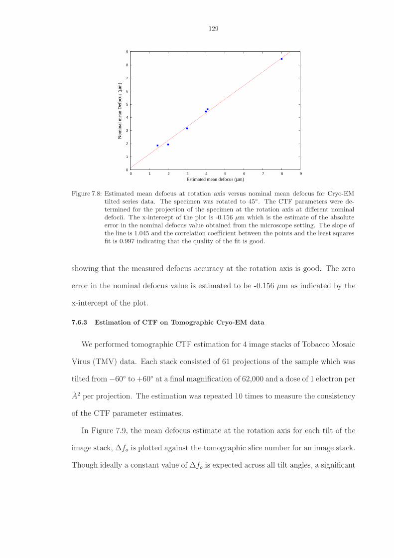
129

0

1

2

3

4

5

6

7

8

9

0 1 2 3 4 5 6 7 8 9

Nom

inal

mea

n D

efoc

us (

µm)

Estimated mean defocus (µm)

Figure 7.8: Estimated mean defocus at rotation axis versus nominal mean defocus for Cryo-EMtilted series data. The specimen was rotated to 45◦. The CTF parameters were de-termined for the projection of the specimen at the rotation axis at different nominaldefocii. The x-intercept of the plot is -0.156 µm which is the estimate of the absoluteerror in the nominal defocus value obtained from the microscope setting. The slope ofthe line is 1.045 and the correlation coefficient between the points and the least squaresfit is 0.997 indicating that the quality of the fit is good.

showing that the measured defocus accuracy at the rotation axis is good. The zero

error in the nominal defocus value is estimated to be -0.156 µm as indicated by the

x-intercept of the plot.

7.6.3 Estimation of CTF on Tomographic Cryo-EM data

We performed tomographic CTF estimation for 4 image stacks of Tobacco Mosaic

Virus (TMV) data. Each stack consisted of 61 projections of the sample which was

tilted from −60◦ to +60◦ at a final magnification of 62,000 and a dose of 1 electron per

A2 per projection. The estimation was repeated 10 times to measure the consistency

of the CTF parameter estimates.

In Figure 7.9, the mean defocus estimate at the rotation axis for each tilt of the

image stack, ∆fo is plotted against the tomographic slice number for an image stack.

Though ideally a constant value of ∆fo is expected across all tilt angles, a significant

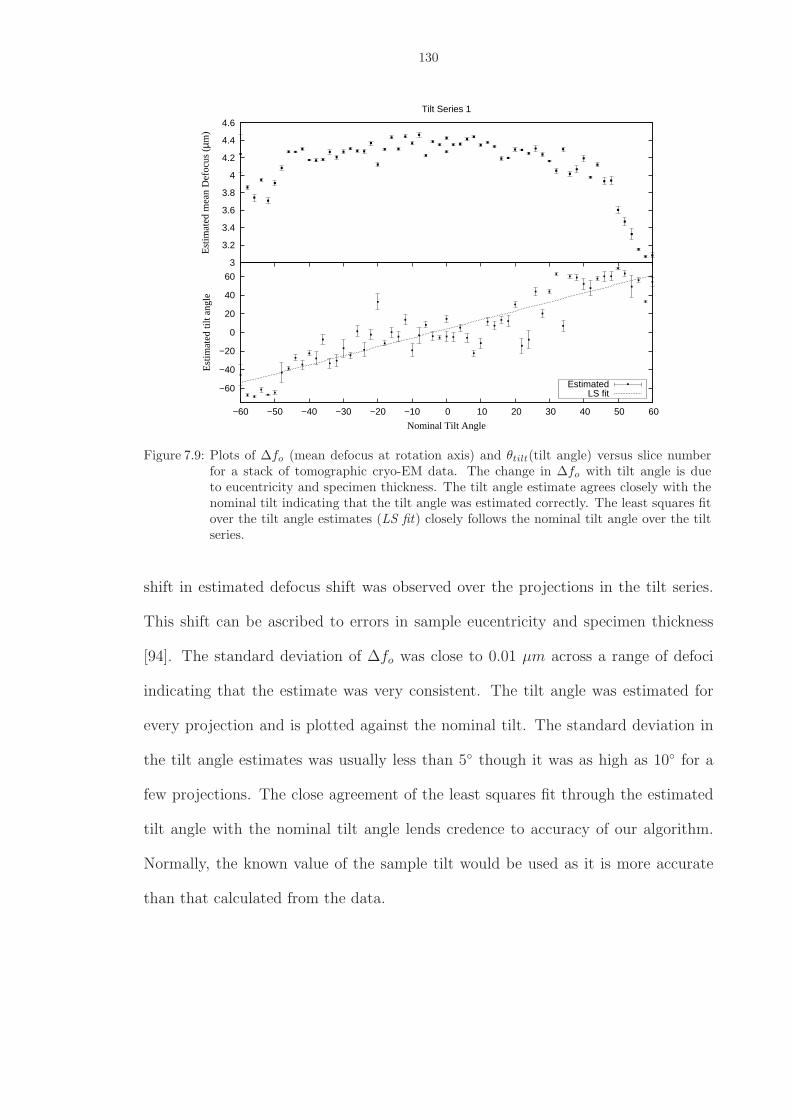
130

3

3.2

3.4

3.6

3.8

4

4.2

4.4

4.6

Est

imat

ed m

ean

Def

ocus

(µm

)

Tilt Series 1

−60

−40

−20

0

20

40

60

−60 −50 −40 −30 −20 −10 0 10 20 30 40 50 60

Est

imat

ed ti

lt an

gle

Nominal Tilt Angle

EstimatedLS fit

Figure 7.9: Plots of ∆fo (mean defocus at rotation axis) and θtilt(tilt angle) versus slice numberfor a stack of tomographic cryo-EM data. The change in ∆fo with tilt angle is dueto eucentricity and specimen thickness. The tilt angle estimate agrees closely with thenominal tilt indicating that the tilt angle was estimated correctly. The least squares fitover the tilt angle estimates (LS fit) closely follows the nominal tilt angle over the tiltseries.

shift in estimated defocus shift was observed over the projections in the tilt series.

This shift can be ascribed to errors in sample eucentricity and specimen thickness

[94]. The standard deviation of ∆fo was close to 0.01 µm across a range of defoci

indicating that the estimate was very consistent. The tilt angle was estimated for

every projection and is plotted against the nominal tilt. The standard deviation in

the tilt angle estimates was usually less than 5◦ though it was as high as 10◦ for a

few projections. The close agreement of the least squares fit through the estimated

tilt angle with the nominal tilt angle lends credence to accuracy of our algorithm.

Normally, the known value of the sample tilt would be used as it is more accurate

than that calculated from the data.

131

7.7 Discussion

We have implemented an automatic CTF estimation algorithm. Unlike other

algorithms [57, 77, 52, 34] the estimation of the defocus parameters is completely done

in 2 dimensions. No initial guess of the CTF is needed as the algorithm generates

an initial guess by performing a coarse grid search covering for the mean defocus,

differential defocus and orientation of the astigmatism over the entire parameter

range in a total of 256 sample points.

For negative stained specimens and for ice samples backed by carbon film, the

algorithm performed quite well. The defocus values were in close agreement to the

values obtained from the algorithms of Tani et al. and Mullick et al. [77, 52]. The

algorithm was also able to accurately measure the mean defocus for protein specimens

embedded in ice without a carbon film. In these cases, astigmatism values should be

taken from adjacent carbon film areas.

Reliable and accurate defocus estimates were found for tilted images, either ran-

dom conical tilt or tomographic data. Due to the low SNR , the tilt angle estimates

for cryo EM tomographic data varied by up to 10◦. However, in practice the tilt

angle is known quite accurately, and thus we can use this information to provide an

even more accurate estimate of ∆fo. At present, the algorithm neither estimates the

amount of amplitude contrast nor does it estimate the envelope function. Reasonable

estimates exist for the magnitude of the amplitude contrast, and to date, the enve-

lope function is not used by CTF correction algorithms. While the current approach

is quite effective, the background estimation step could be further improved, perhaps

by using limited Bessel functions to minimize the number of parameters, but allow

smooth variation with angle. We are presently working on alternative optimization

132

functions and improved handling of envelope and background functions.

The program was developed on Python, an open source platform, and is freely

available from the authors.

CHAPTER VIII

Edge-preserving deconvolution for cryo-electron microscopy

images

8.1 Introduction

Cryo-electron microscopy (cryo-EM) is a powerful method for observing macro-

molecular complexes in their native states. Under typical conditions, cryo specimens

are imaged at moderate values of defocus to produce sufficient contrast. While neces-

sary, the defocus and spherical aberration of the objective lens introduce significant

distortions into the image that must subsequently be corrected. The image formation

process can be mathematically modeled as a convolution of the object being imaged

with the imaging system’s Contrast Transfer Function (CTF), which characterizes

the fidelity by which spatial information is transferred from input to output across

a range of spatial frequencies [52, 72, 14, 57]. As a result, deconvolving the image by

the CTF - or “CTF correction” - is essential for obtaining accurate, high-resolution

object information [14].

Typically, images are deconvolved using one of two approaches: (1) phase flip-

ping algorithms, that deconvolve the image by assuming the CTF has a constant

amplitude and (2) algorithms such as Wiener filters which attempt to correct for

amplitude and phase changes, Such simple linear filters can be considered as mem-

bers of a more general class of regularized least squares deconvolution algorithms

133

134

[49, 56, 14, 19, 6]. Regularization refers to the inclusion of information about the

object being imaged in order to obtain a stable and useful solution [63]. Both phase

flipping and Wiener filtering suffer from significant drawbacks. On the one hand,

phase flipping does not correct for the amplitude distortions due to the CTF thereby

underemphasizing selective spatial frequencies in the reconstruction. On the other

hand, most regularized least squares methods such as Wiener filters and quadratic

gradient regularizers tend to yield oversmooth solutions that blur out object edges

[39, 31, 27, 17]. While algorithms that combine Wiener filtering and phase flipping

have been proposed [56, 80], they ultimately suffer from the same problems. Hence,

there is a need for an algorithm that deconvolves the image by the CTF and at the

same time, optimally preserves high frequency object information.

While the application of deconvolution algorithms for resolution enhancement

is relatively new to electron microscopy, it is a well established technique in the

signal processing and astronomy community with a history of over 30 years [48, 69,

76]. Recently, a new class of myopic, edge-preserving deconvolution algorithms have

been developed that perform demonstrably better than conventional methods for

astronomical and optical images [59, 31]. However, until now, these algorithms have

not been applied to EM images.

In this chapter, we present an edge-preserving deconvolution algorithm that cor-

rects for the phase and amplitude effects of the CTF and preserves the edges of the

object being imaged. First, we briefly review the phase image formation process in

EM. Second, we discuss our CTF correction strategy in a mathematical framework.

Finally, we describe the methodology of our experiments and demonstrate that our

algorithm corrects images by the CTF better than phase flipping with amplitude

correction, Wiener filtering and their variants over most resolutions.

135

8.2 Theory of Image Formation and CTF Correction

8.2.1 Image Formation

The EM phase image formation process is described by the theory of contrast

transfer as

(8.1) i(r, θ) = h(r) ⊗ o(r) ⊗ e(r) + n

where r is the vector of co-ordinates and i,h and o are the image, transfer function

of the system and object respectively. The ⊗ operator describes the convolution op-

eration. e(r) represents a Gaussian-like function known as the envelope function that

describes the reduction in image contrast with increasing spatial frequency due to

the coherence of the electron beam, lens current instability, stage drift and measured

modulation transfer function (MTF) of the detector [67]. We assume the noise in the

system, n is a combination of Poisson noise due to electron-detection and Gaussian

noise, e.g., due to detector or scanner electronics and approximate both by using the

mixed Gaussian model [46, 31].

Applying the Fourier transform to (8.1) we get

(8.2) I(q) = CTF (q)O(q)E(q) + N

where the term CTF (q) is the contrast transfer function, the Fourier transform

of h(r).

The CTF is theoretically well characterized for thin samples and using the weak-

phase-weak-amplitude approximation can be expressed as:

(8.3) CTF (q) =√

1 − α2 sin χ(q) − α cos χ(q)

136

where α is an amplitude contrast factor ( 0 ≤ α ≤ 1) and χ(q) is the scatter-

ing angle dependent path length difference of the electron wavefront [67]. χ is a

parametric function of the spherical aberration of the objective lens, wavelength of

electron beam and defocus and astigmatism parameters of the CTF. Thus, the CTF

is usually known to a high degree of accuracy as these parameters are either provided

by the manufacturer or can be easily determined using CTF estimation algorithms

[72, 52, 57, 77].

8.2.2 Deconvolution

As seen in (8.2), the EM image can be considered as a representation of the

object distorted by the CTF and the envelope function. In this chapter, we focus

only on correcting the errors introduced by the CTF , and thus aim to recover the

envelope function filtered version of the object, Oe(q) = O(q)E(q) from the image.

Our concern was that since the envelope function is small at the higher frequencies,

its deconvolution could lead to an amplification of high frequency signals where the

noise power spectrum dominates the signal power spectrum leading to unstable and

noisy object estimates [14].

There are two common deconvolution strategies currently used to process EM

imaging data. The first, phase flipping, corrects for the phase effects of the CTF by

reversing the phase of the image Fourier transform in regions of the frequency plane

where the CTF is negative. This approach implicitly assumes that the amplitude

of the CTF is a non-zero constant at all frequencies; although conservative, this

assumption is, of course, not accurate. The second class of methods correct for the

CTF in a regularized least squares framework. Here, the object estimate oe(r) is

given by that choice of oe(r) which minimizes

137

(8.4) ‖i(r) − oe(r) ⊗ h(r)‖2 + λRR

Here, λR is a constant known as the regularization parameter and R is the reg-

ularization factor. When R = ‖oe(r)‖2, we aim to keep the object estimate oe(r)

small by penalizing large solutions of oe(r). For this choice of R, the object estimate

minimizing (8.4) can be expressed as,

(8.5) oe(r) = FT−1(I(q)W (q))

where

(8.6) W (q) =CTF ∗(q)

| CTF (q) |2 +λR

is known as the Wiener filter [6, 95, 50].

Other choices for R are empirically derived from the observation that natural

object surfaces are generally smooth with constant or slowly changing intensities

between pixels where as noisy areas are discontinuous exhibiting a rapid change of

intensities in neighboring pixels. This property is quantified by the norm of the

spatial gradient of the object defined as

(8.7) ‖∇o(r)‖ =[(∇ox(r))

2 + (∇oy(r))2] 1

2

The choices R = 12

∑

r

‖∇oe(r)‖2 and R =∑

r

‖∇oe(r)‖ represent quadratic and

linear gradient regularizers which penalize gradients in the image.

138

Edge-Preserving regularizer

While, both Wiener filtering and quadratic gradient regularizers are effective in

smoothing out noise, they tend overcompensate for large gradients caused by edges

thereby unnecessarily blurring them. In contrast, linear gradient regularizers do not

sufficiently suppress noise, but are effective in preserving edges as they do not over-

penalize large gradients. Another class of functions, known as Huber functions over-

come this problem and act as edge-preserving regularizers by behaving like quadratic

gradient regularizers for small gradients and as less severe linear gradient regularizers

for large gradients [11]. We use the function originally proposed by Brette and Idier

and implemented by Hom et al [7, 31].

(8.8) R =∑

r

γ − ln(1 + γ)

(8.9) γ = (‖∇oe(r)‖

β(r))

Here γ is the reduced gradient modulus. When γ is small, γ − ln(1 + γ) ≈ γ2/2

and when γ is large γ − ln(1 + γ) ≈ γ . Thus, R behaves like a quadratic gradient

regularizer when γ is small and as a linear gradient regularizer when γ is large. The

terms β(r) and λR from Eqs. (8.8) and (8.4) are known as the hyperparameters of

the object and can be determined automatically. The scheme for estimating these

hyperparameters is discussed in greater detail by Hom et al [31].

We note that due to the non-linearity of edge-preserving regularizers, analytical

solutions that minimize (8.4) do not exist in general [17]. This necessiates the use

of iterative optimization algorithms such as Conjugate Gradients [23] to calculate

oe(r).

139

For the sake of brevity, we shall refer to the deconvolution using the edge pre-

serving regularizer and the quadratic gradient regularizer as the edge-preserving al-

gorithm and the quadratic gradient algorithm respectively.

8.3 Methods

The structure of the R-type bacterial flagella filament was recently resolved to

atomic resolution [93] and thus provides an excellent test specimen for exploring im-

age processing methodology. The filament is shaped roughly like a hollow cylinder

and made up of helically repeating subunits. The overall architecture is an outer

projection and a densely packed core region comprised of two concentric tubes sur-

rounding a central channel, each tube being made up of α-helices running almost

parallel to the filament axis.

We compared helical 3-D reconstructions of the R-type bacterial flagellar filament

after deconvolving the primary cryo-micrographs using either the edge preserving

algorithm or other more conventional techniques with the atomic structure. The

reconstructions were qualitatively examined by visual inspection of the core regions

and quantitatively compared using amplitude-weighted phase residuals [2] between

the deconvolved reconstructions and the reference atomic model.

8.3.1 Sample Preparation and Acquisition

Five cryo-EM micrographs, each containing several straight R-type bacterial flag-

ellar filament images were acquired using an FEI Polara TF-30 Electron Microscope

operating at 300 KeV equipped with an UltraCam lens-coupled CCD camera and a

post-column energy filter [90]. The chip size of the CCD array was 4096 × 4096. The

images were acquired at a final magnification of 113,000 X at a sampling resolution

of 1.33 A/pixel.

140

8.3.2 Image Processing of Individual Samples

Images of five filaments, each filament containing 400 subunits, were isolated

from the micrographs. After determining the CTF parameters from the micrographs

using the algorithm of Shah et al. [72], each image was deconvolved using the fol-

lowing methods: (1) the edge-preserving algorithm, (2) phase flipping, (3) phase

flipping with amplitude correction [80, 56], (4) Wiener filtering, (5) least squares

without regularization, and (6) the quadratic gradient least squares algorithm. In

the case of the edge-preserving and the quadratic gradient least squares algorithms,

(8.4) was minimized using a Constrained Conjugate Gradients algorithm [23] in the

framework of the AIDA image deconvolution algorithm [31]. In this framework, the

edge-preserving algorithm required approximately 2 minutes for the deconvolution

of a 512 by 512 image on a 3 GHz, Pentium 4 computer. The flagella filament

was reconstructed in 3-D with the deconvolved images at 10 A resolution using the

method described by Yonekura et al. [90]. Figure 8.1 describes the deconvolution

and reconstruction process.

8.3.3 Quantitative Analysis

Due to the helically repeating structure, the Fourier transform of bacterial flagellar

filaments can be described in terms of a set of Fourier-Bessel layer lines parallel to

the equator [56]. The amplitude weighted phase difference between layer-line data

of the object and the reference data (calculated from the atomic model) at a given

resolution is known as the phase residual error [85, 2]. A low phase error indicates a

high degree of similarity between the object and the reference data. Phase residuals

become large when noise overwhelms the layer-line information. Here, a phase error

of 70◦ is considered as the noise threshold beyond which the signal is assumed to

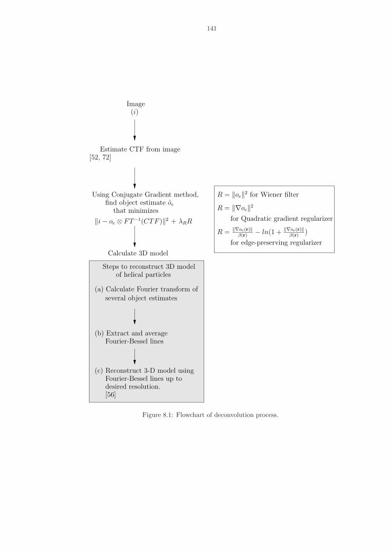
141

for Quadratic gradient regularizer

Steps to reconstruct 3D modelof helical particles

(b) Extract and average

[56]

Fourier-Bessel lines

Fourier-Bessel lines up todesired resolution.

R = ‖∇oe‖2

R = ‖∇oe(r)‖β(r)

− ln(1 + ‖∇oe(r)‖β(r)

)

R = ‖oe‖2 for Wiener filter

for edge-preserving regularizer

Estimate CTF from image

(a) Calculate Fourier transform of

several object estimates

(c) Reconstruct 3-D model using

(i)Image

[52, 72]

Using Conjugate Gradient method,

that minimizes

‖i − oe ⊗ FT−1(CTF )‖2 + λRR

find object estimate oe

Calculate 3D model

Figure 8.1: Flowchart of deconvolution process.

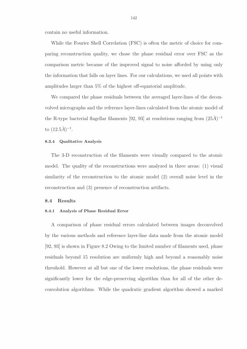
142

contain no useful information.

While the Fourier Shell Correlation (FSC) is often the metric of choice for com-

paring reconstruction quality, we chose the phase residual error over FSC as the

comparison metric because of the improved signal to noise afforded by using only

the information that falls on layer lines. For our calculations, we used all points with

amplitudes larger than 5% of the highest off-equatorial amplitude.

We compared the phase residuals between the averaged layer-lines of the decon-

volved micrographs and the reference layer-lines calculated from the atomic model of

the R-type bacterial flagellar filaments [92, 93] at resolutions ranging from (25A)−1

to (12.5A)−1.

8.3.4 Qualitative Analysis

The 3-D reconstruction of the filaments were visually compared to the atomic

model. The quality of the reconstructions were analyzed in three areas: (1) visual

similarity of the reconstruction to the atomic model (2) overall noise level in the

reconstruction and (3) presence of reconstruction artifacts.

8.4 Results

8.4.1 Analysis of Phase Residual Error

A comparison of phase residual errors calculated between images deconvolved

by the various methods and reference layer-line data made from the atomic model

[92, 93] is shown in Figure 8.2 Owing to the limited number of filaments used, phase

residuals beyond 15 resolution are uniformly high and beyond a reasonably noise

threshold. However at all but one of the lower resolutions, the phase residuals were

significantly lower for the edge-preserving algorithm than for all of the other de-

convolution algorithms. While the quadratic gradient algorithm showed a marked

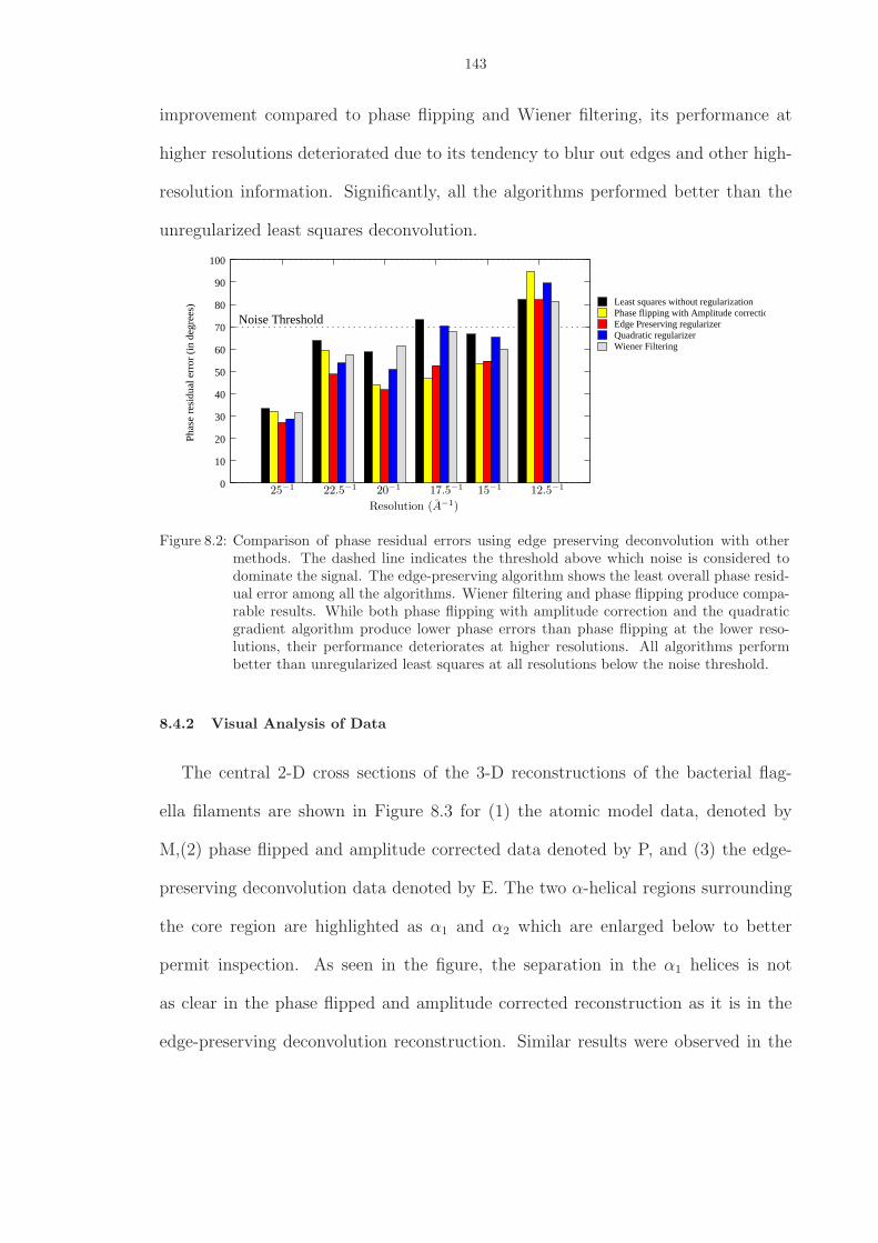
143

improvement compared to phase flipping and Wiener filtering, its performance at

higher resolutions deteriorated due to its tendency to blur out edges and other high-

resolution information. Significantly, all the algorithms performed better than the

unregularized least squares deconvolution.

Phase flipping with Amplitude correctionEdge Preserving regularizerQuadratic regularizerWiener Filtering

Least squares without regularization

Noise Threshold

60

40

30

10

20

0

70

80

90

100

Phas

e re

sidu

al e

rror

(in

deg

rees

)

50

12.5−125−1 22.5−1 20−1 17.5−1 15−1

Resolution (A−1)

Figure 8.2: Comparison of phase residual errors using edge preserving deconvolution with othermethods. The dashed line indicates the threshold above which noise is considered todominate the signal. The edge-preserving algorithm shows the least overall phase resid-ual error among all the algorithms. Wiener filtering and phase flipping produce compa-rable results. While both phase flipping with amplitude correction and the quadraticgradient algorithm produce lower phase errors than phase flipping at the lower reso-lutions, their performance deteriorates at higher resolutions. All algorithms performbetter than unregularized least squares at all resolutions below the noise threshold.

8.4.2 Visual Analysis of Data

The central 2-D cross sections of the 3-D reconstructions of the bacterial flag-

ella filaments are shown in Figure 8.3 for (1) the atomic model data, denoted by

M,(2) phase flipped and amplitude corrected data denoted by P, and (3) the edge-

preserving deconvolution data denoted by E. The two α-helical regions surrounding

the core region are highlighted as α1 and α2 which are enlarged below to better

permit inspection. As seen in the figure, the separation in the α1 helices is not

as clear in the phase flipped and amplitude corrected reconstruction as it is in the

edge-preserving deconvolution reconstruction. Similar results were observed in the

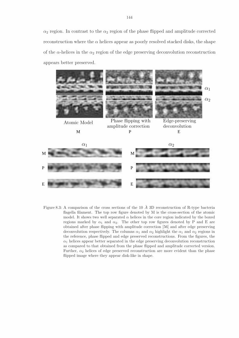
144

α2 region. In contrast to the α2 region of the phase flipped and amplitude corrected

reconstruction where the α helices appear as poorly resolved stacked disks, the shape

of the α-helices in the α2 region of the edge preserving deconvolution reconstruction

appears better preserved.

P

E

M

P

E

M P E

M

α2α1

deconvolution

α1

amplitude correction

α2

Phase flipping with Edge-preservingAtomic Model

Figure 8.3: A comparison of the cross sections of the 10 A 3D reconstruction of R-type bacteriaflagella filament. The top row figure denoted by M is the cross-section of the atomicmodel. It shows two well separated α helices in the core region indicated by the boxedregions marked by α1 and α2. The other top row figures denoted by P and E areobtained after phase flipping with amplitude correction [56] and after edge preservingdeconvolution respectively. The columns α1 and α2 highlight the α1 and α2 regions inthe reference, phase flipped and edge preserved reconstructions. From the figures, theα1 helices appear better separated in the edge preserving deconvolution reconstructionas compared to that obtained from the phase flipped and amplitude corrected version.Further, α2 helices of edge preserved reconstruction are more evident than the phaseflipped image where they appear disk-like in shape.

145

8.5 Discussion

CTF deconvolution is essential to obtain high-resolution information in cryo-EM.

The challenge is to optimally correct for the aberrations introduced by the CTF but

to minimize noise amplification. The latter problem is especially significant given

the very low signal-to-noise ratio for cryo-EM images. While traditional methods

succeed in correcting some of the phase and amplitude effects of the CTF they also

introduce artifacts such as oversmooth object edges or they may poorly suppress

noise.

We have presented a deconvolution algorithm in the regularized least squares

framework that aims to perform both amplitude and phase correction of the CTF

while at the same time preserves object edge information and suppresses noise. This

is achieved by using a regularizer that behaves like a quadratic gradient regular-

izer for small gradients, thus suppressing noise, and like a linear gradient regularizer

when the gradients are large, thereby preserving edges. Both qualitative and quanti-

tative results indicate that this method produces better results than phase flipping,

phase flipping with amplitude correction, Wiener filtering and quadratic gradient

regularized deconvolution algorithms.

The algorithm presented in this chapter performs deconvolution on individual 2-D

projections before the 3-D reconstruction. A significant advantage of this approach

is that operations such as classification and alignment should be greatly facilitated

by more accurate image data. While a potential drawback is that any artifacts in-

troduced during the deconvolution stage would be present in the 3-D reconstruction,

the results presented here indicate that our approach is considerably more accu-

rate than the alternative methods such as phase flipping or Weiner filtering. Thus

146

edge-preserving deconvolution should be considered a robust alternative to more con-

ventional CTF correction schemes performed on individual images. A better, albeit

more time consuming, approach would be to perform CTF deconvolution as part

of the 3-D reconstruction process as demonstrated by Zhu et al. [49] and include

edge-preserving regularization to preserve object properties and control noise am-

plification. We aim to combine the deconvolution and reconstruction steps in the

future.

While estimating the electron coherence envelope function can be problematic

with cryo-images because it is multiplied by the power spectrum of the sample or

carbon-film, the detector MTF is well characterized and can be measured to a high

degree of accuracy [49]. As a consequence, including the detector MTF in the overall

deconvolution algorithm should provide a relatively simple way to further enhance

the results. This is likely to be important when using CCD detectors as their MTFs

vary more dramatically with spatial resolution than does film. Once measured, the

MTF could be included in the problem formulation along with the CTF to deconvolve

out from the image.

CTF deconvolution offers the potential to extend the useful resolution of tomo-

graphic and tilted cryo-EM data such as collected for conical tilt reconstructions.

Unfortunately, tomographic CTFs vary across the image plane making the deconvo-

lution problem more challenging. Presently, there are two approaches to overcome

this issue. The first divides the tilted image into stripes parallel to the rotation axis

where the CTF is assumed constant and each section is deconvolved. This approach

is problematic for images that are tilted to high angles where the approximation

of CTF constancy requires many narrow stripes leading to edge artifacts that can

be enhanced by the deconvolution process. Another approach is to perform one-

147

dimensional deconvolution along stripes parallel to the tilt axis fully accounting for

the defocus variation in the CTF due to the tilt [86]. This method assumes that

astigmatism is absent in the imaging system.

We are presently adapting the algorithm to account for the MTF and are also

directing our efforts in the area of edge preserving deconvolution for cryo-tomographic

data.

CHAPTER IX

Conclusion

This thesis can be divided into two parts in terms of approach. In the first part

we developed two algorithms for blind deconvolution of images, with an aim to use

them for incoherent bio-imaging applications, such as fluorescence microscopy. The

first algorithm was developed for imaging systems with even PSFs. Such PSFs are

common in optical and fluorescence microscopy. We then extended this algorithm

to the 3-D case. Next, we developed a blind deconvolution algorithm based on the

QUILL image model, and demonstrated its effectiveness on a variety of images.

The second part of the thesis was primarily concerned with electron microscopy.

Two algorithms have also been developed and deployed here. The first algorithm

was developed to determine the Contrast Transfer Function (CTF) of electron mi-

croscopes automatically from planar and tomographic EM images. The second al-

gorithm was based on an edge-preserving algorithm first demonstrated by Mugnier

et al. [59] and later by Hom et al. [31] in the context of optical microscopy and

astronomy.

In this final section, we briefly review the pros and cons of the algorithms described

in this thesis. Potential extensions of these methods are discussed next.

148

149

9.1 Current State of the Algorithms

9.1.1 Blind Even-PSF Deconvolution

The algorithms presented in Chapters III and IV aimed to perform blind decon-

volution of 2-D and 3-D images that were convolved with an even PSF. The only

assumptions made were the support size of the PSF was known and that the image

has finite support. Unlike most other blind deconvolution algorithms that have been

developed, this algorithm was non-iterative. The only problem with the algorithm

formulation was that it was intractable for medium and large sized 2-D images, and

almost all 3-D images. This problem was overcome using the Fourier decoupling

approach, which simplified the problem from a single large 2-D or 3-D problem to

several simple 1-D problems. The only drawback with using Fourier decomposition

is that the Mean Square Error (MSE) is slightly increased with respect to the direct

approach, due to the necessity of determining scale factors.

However, from both theoretical and practical perspectives, there are a few draw-

backs. First, the decoupled version of the algorithm is more sensitive to errors. Here,

a bad result in one of the 1-D problems manifests itself in the overall reconstruction

during to the recoupling process. Second, the finite support constraint precludes its

use in many microscopy applications, where the structures being observed do not

have finite support. Third, in most cases, the PSF is not truly symmetric due to lens

defects.

Fortunately, PSF symmetry can be assumed for low resolution imaging, since the

approximation of symmetry has little effect on the overall reconstruction result at

low resolutions. We also note that these algorithms are more applicable in areas such

as astronomy, where images having compact support are common (e.g., a nebula on

a black background).

150

9.1.2 Blind Deconvolution using QUILL

Chapter V discussed the QUILL-model-based blind deconvolution algorithm. The

key assumption here is that the QUILL model is a reasonably good approximation of

the object, and that the support size of the PSF is known. This algorithm is also non-

iterative, and fast as most of the unknown pixels are found by simple convolution.

Unlike the previous algorithm, it can also handle the partial data case (i.e. compact

support is not required).

The chief drawback of this method is that many realistic microscopic images do not

fit the model very well. This is especially true in high resolution imaging. However,

we note that in high speed microscopy objects are often viewed at low resolution and

the images thus formed should be modeled well by QUILL.

9.1.3 Contrast Transfer Function (CTF) Estimation Algorithm

While the CTF estimation algorithm discussed in Chapter VI is not the first

algorithm in its class, it incorporates many features that make it unique. First, it

is one a rare class of fully automatic CTF estimation algorithms for cryo-electron

microscopy. This is achieved by using several novel CTF pre-processing steps that

eliminate the need for manual input. Second, it is the only algorithm that can

estimate the CTF parameters of tilted images. This is a significantly harder problem

than the planar image case, as the CTF for a tilted image changes across the imaging

plane. Third, the program is user-friendly, and has been developed on an Open

Source platform that makes it easily extensable for future work.

This algorithm can be improved by changing some of the pre-processing steps.

The background fitting is presently done in an inelegant partial 2-D curve-fit. A

better approach would be to use a fully 2-D approach. We also note that while the

151

background is modeled as an additive component in the observed CTF, we use a least

squares fit that minimizes the sum of squares of the fit with respect to the observed

CTF. As a result, the estimated background can be larger at times than the observed

CTF. Subtracting of the estimated background often leads to spurious negatively-

valued areas in the residual CTF that is used for estimation. This is theoretically

incorrect and needs to be rectified.

9.1.4 Deconvolution of EM Images using the edge-preservation Algorithm

The algorithm presented in this paper is an attempt to deconvolve EM images

using an edge-preserving regularizer. Our preliminary results indicate that the al-

gorithm performs better than other commonly used “CTF correction” approaches.

The algorithm is automatic, and does not need any user input apart from the CTF

parameters, which can also be estimated automatically using the previous algorithm.

The main drawback of this algorithm is that it does not include the envelope

function as part of the formulation. This might play a significant role at higher

resolutions. Unfortunately, due to the low SNR of the sample-set on which the

deconvolution was tried, the deconvolution would have amplified high-frequency noise

more than it would have restored the object, and consequently would have degraded

performance significantly.

While all of the algorithms discussed above have drawbacks, there are several

ways in which they could be improved. We discuss some of these, along with more

ambitious ideas, in the next section.

152

9.2 Future Work

9.2.1 Deployment of Blind Deconvolution Algorithms for Fluorescence MicroscopyApplications

While both the symmetric PSF algorithm and the QUILL algorithm have shown

very promising simulation results, they have yet to be tested on a large number of

real deconvolution problems. The symmetric PSF algorithm is well-suited for imag-

ing systems that show small or almost no spherical aberrations, so that the PSF

symmetry is maintained. The QUILL algorithm requires that the object be heav-

ily oversampled so that subsequent undersampling does not affect the deconvolution

significantly. For this reason, the QUILL algorithm is a good candidate for deconvo-

lution of high speed confocal microscopy images, where the emphasis is not only on

performance of the deconvolution algorithm, but also on time taken to deconvolve

the image.

9.2.2 Choice of a Different Regularizer for QUILL Algorithm

The QUILL algorithm was demonstrated using a Truncated Singular Value De-

composition method for regularization [63]. The TSVD method is closely related

to the Tikhonov method, and is essentially a linear regularization method. These

class of methods, while fast, suffer from the resolution-noise tradeoff problem, i.e.,

if one increases the contribution of the regularizer to remove noise, then the over-

all image appears blurry. A better way to regularize would be to use a non-linear

edge-preserving regularizer, which attempts to remove noise, while at the same time

preserving image edges [17].

9.2.3 Improvements and Extensions to CTF Estimation Algorithm

The CTF estimation algorithm can be improved in three key ways.

First, the background estimation step, which is presently done as a partial 2-D

153

problem, could be implemented as a 2-D curve-fit problem, where a 2-D polynomial

could be fit over the entire fit area.

Second, the envelope function and background estimation step is presently fitted

using a least squares fit. Given that the background is modelled as an additive func-

tion in the observed CTF, the background will be better estimated as a constrained

least squares problem, where the upper bound of the fit is the observed CTF.

Third, the algorithm does not calculate the envelope function of the CTF. This

can easily be done using a constrained least squares approach.

Another related potential area of improvement would be to provide a better graph-

ics front end for ease of use for electron microscopists.

9.2.4 Improvements to the Edge-Preserving Deconvolution Algorithm

While the edge-preserving algorithm presented in Chapter VI is promising, the

results presented are only preliminary. It needs to be applied to the deconvolution

of a variety of structures to be accepted in the EM community. There are also three

ways in which the algorithm may be improved.

First, the envelope function must be part of the problem formulation. While the

envelope function does not play a big role at lower resolutions, where it is mostly

flat, it rapidly decays at the higher resolutions affecting the high-frequency object

information. One way to incorporate this would be use many more images (50-100),

so that the SNR of the data at high resolutions is good enough to deconvolve by the

envelope function.

Second, unlike AIDA or MISTRAL [31, 59], the algorithm is not myopic. Given

that CTF estimation may yield transfer function parameters that are not as accurate

[52], a myopic approach to deconvolution may correct the CTF slightly to give a

better object estimate.

154

Third, and perhaps most ambitious, is that algorithm could be adapted for use

for tomographic data. This is especially difficult because the CTF changes across the

imaging plane, so the deconvolution is no longer spatially invariant. Two approaches

currently exist to deal with this issue, both making approximations to simplify the

problem. One approach breaks up the imaging plane where the CTF is assumed

constant in each plane, while the other approach assumes the CTF does not have

astigmatism [86]. If it is possible to model the problem where the CTF and image

over the entire plane are considered, the solution, apart from being more elegant,

would theoretically be better.

Several potential future improvements discussed here are challenging. However,

they offer the promise of being rewarding, especially to the microscopy community.

APPENDICES

155

156

APPENDIX A

Derivation of tomographic CTF formula

We assume the origin of the coordinates is at the center of the object plane and

is marked by O. Os is the center of the specimen plane. The sample is tilted by

θtilt with respect to the object plane. The rotation axis r′ passes through Os and is

rotated θrot with respect to the y-axis, as shown in Fig. (A.1). The mean defocus of

a point is defined as the distance of the point on the specimen plane to the object

plane. So, the z-ordinate ∆fo of Os denotes the mean defocus at the rotation axis.

U(x1, y1, z1) is an arbitrary point on the specimen where we wish to measure the

mean defocus. If p(x1, y1, θrot) is the projection of the distance between a point on

the specimen plane and the rotation axis on the zero tilt plane, then

(A.1) p(x1, y1, θrot) = x1 cos θrot + y1 sin θrot

∆f and p(x1, y1, θrot) are related as

(A.2) ∆f = p(x1, y1, θrot) tan θtilt

The defocus at U(x1, y1, z1) is

(A.3) ∆fx1,y1,z1≡ z1 = ∆f + ∆fo

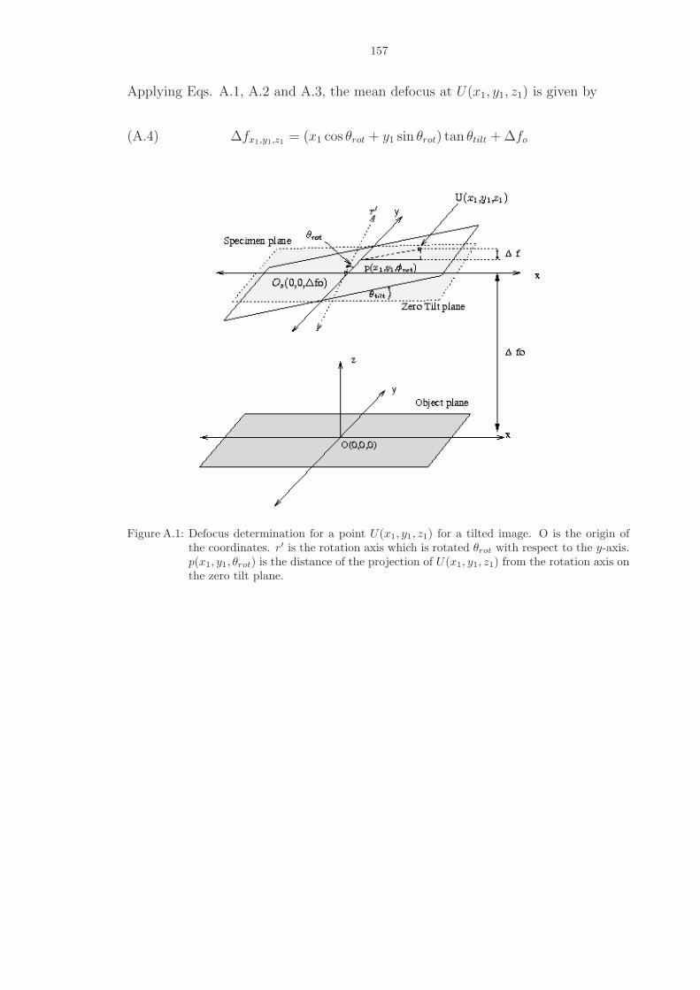
157

Applying Eqs. A.1, A.2 and A.3, the mean defocus at U(x1, y1, z1) is given by

(A.4) ∆fx1,y1,z1= (x1 cos θrot + y1 sin θrot) tan θtilt + ∆fo

Figure A.1: Defocus determination for a point U(x1, y1, z1) for a tilted image. O is the origin ofthe coordinates. r′ is the rotation axis which is rotated θrot with respect to the y-axis.p(x1, y1, θrot) is the distance of the projection of U(x1, y1, z1) from the rotation axis onthe zero tilt plane.

BIBLIOGRAPHY

158

159

BIBLIOGRAPHY

[1] D. Agard, “Optical sectioning microscopy: cellular architecture in three dimensions,” AnnualReviews in Biophysics and Bioengineering, vol. 13, pp. 191–219, 1984.

[2] L. Amos and A. Klug, “Three-dimensional image reconstruction of the contractile tail of T4bacteriophage,” Journal of Molecular Biology, vol. 99, pp. 51–73, 1975.

[3] Andrews and Hunt, “Digital image restoration,” Prentice Hall, 1974.

[4] R. Aster, B. Borchers, and C. Thurber, “Parameter estimation and inverse problems,” ElselvierAcademic Press, 2004.

[5] J. Besag, “On the statistical-analysis of dirty pictures,” J Royal Statistical Society B, vol. 48,pp. 259–302, 1986.

[6] J. Biemond, R. L. Lagendijk, and R. M. Mersereau, “Iterative methods for image deblurring,”Proceedings of the IEEE, 1990.

[7] S. Brette and J. Idier, “Optimized single site update algorithms for image deblurring,” ImageProcessing, Proceedings., International Conference on, vol. 3, pp. 65–68, 1996.

[8] J. Cadzow, “Signal enhancement-a composite property mapping algorithm,” IEEE Transac-tions on Signal Processing, vol. 36, no. 1, pp. 49–63, 1988.

[9] A. Carasso, “Linear and nonlinear image deblurring: A documented study,” SIAM Journal onNumerical Analysis, vol. 36, no. 6, pp. 1659–1689, 1999.

[10] P. Charbonnier, L. Blanc-Feraud, G. Aubert, and M. Barlaud, “Deterministic edge-preservingregularization in computed imaging,” IEEE Transactions on Signal Processing, vol. 44, no. 10,pp. 2464–2474, 1996.

[11] ——, “Deterministic edge preserving regularization in computed imaging,” IEEE Transactionsin Image Processing, vol. 6, no. 2, pp. 298–311, 1996.

[12] J. Conan, L. Mugnier, T. Fusco, V. Michau, and G. Rousset, “Myopic deconvolution of adaptiveoptics images by use of object and point-spread function power spectra,” Appl. Opt., vol. 37,pp. 4814–4622, 1998.

[13] J. Conchello and J. McNally, “Fast regularization technique for expectation maximizationalgorithm for optical sectioning microscopy,” Symp. Electronic Imaging Sci. Technol. San Jose,CA 2655, pp. 199–208, 1996.

[14] J. F. Conway and A. C. Steven, “Methods for reconstructing density maps of ”‘single”’ particlesfrom cryoelectron micrographs to subnanometer resolution,” Nature, vol. 424, pp. 643–650,2003.

[15] H. P. Erikson and A. Klug, “The fourier transform of an electron micrograph: Effects ofdefocussing and aberrations, and implications for the use of underfocus contrast enhancement,”Ber. Bunsenges. Phys. Chem., 1970.

160

[16] J.-J. Fernandez, J. R. Fernandez, and J.-M. Fernandez, “A spectral estimation approach tocontrast transfer function detection in electron microscopy,” Ultramicroscopy, 1997.

[17] J. Fessler, Image Reconstruction: Algorithms and Analysis. Book in Preparation, 2006.

[18] J. Fienup, “Phase retrieval algorithms: A comparison,” Appl. Opt., vol. 21, pp. 2758–2769,1982.

[19] J. Frank, M. Radermacher, P. Penczek, J. Zhu, Y. Li, M. Ladjadj, and A. Leith, “SPIDER andWEB: Processing and visualization of images in 3D electron microscopy and related fields,”Journal of Structural Biology, vol. 116, no. 1, pp. 190–199, 1996.

[20] T. Fusco, J. P. Veran, J. Conan, and L. Mugnier, “Myopic deconvolution method for adaptiveoptics images of stellar fields,” Astron. Astrophys. Suppl. Ser., vol. 134, pp. 193–200, 1999.

[21] G. GB and H. RW, “Blind identification of multichannel fir blurs and perfect image resotra-tion,” IEEE Transactions on Image Processing, vol. 9, no. 11, pp. 1877–1896, 2000.

[22] S. Geman and D. Geman, “Stochastic relaxation, gibbs distribution and bayesian restorationof images,” IEEE Trans. Pattern Anal. Mach. Intell., vol. 6, no. 721-741, 1984.

[23] D. M. Goodman, E. M. Johansson, and T. W. Lawrence, “On applying the conjugate gradientalgorihm to image processing problems, chapter 11,” Multivariate Analysis: Future Directions:North-Holland Series inStatistics and Probability, vol. 5, pp. 209–232, 1993.

[24] A. GR and D. JC, “Iterative blind deconvolution method and its applications,” Optics letters,vol. 13, no. 7, pp. 547–549, 1988.

[25] P. Hansen, “Regularization tools for matlab 6.0,” software, vol. ver 3.1.

[26] K. J. Hanzen, “The optical transfer theory of the elctron microscope: fundamental principlesand applications,” Advanced Optical and Electron Microscopy, vol. 4, pp. 1–84, 1971.

[27] G. Harikumar and Y. Bresler, “FIR perfect signal reconstruction from multiple convolu-tions:minimum deconvolver orders,” IEEE Transactions on Signal Processing, vol. 46, no. 1,pp. 215–218, 1998.

[28] ——, “Perfect blind restoration of images blurred by multiple filters: Theory and efficientalgorithms,” IEEE Transactions on Image Processing, vol. 8, no. 2, pp. 202–219, 1999.

[29] T. Holmes, S. Bhattacharya, J. Cooper, D. Hanzel, V. Krishnamurthi, W. Linand, B. Roysam,D. Szaowski, and J. Turner, “Light microscopic images reconstructed by maximum liklihooddeconvolution,” Handbook of Biological and Confocal Microscopy, vol. 2, 1995.

[30] T. Holmes and N. O’Connor, “Blind deconvolution of 3d transmitted light brightfield micro-graphs,” Journal of Microscopy, vol. 200, no. 2, pp. 114–127, 2000.

[31] E. Hom, F. Marchis, S. Haase, T. Lee, D. A. Agard, and J. W. Sedat, “AIDA: An adaptiveimage deconvolution algorithm with application to multi frame and three-dimensional data,”in preparation, 2006.

[32] T. Homes, “Maximum-likelihood image restoration adapted for noncoherent optical imaging,”Journal of the Optical Society of America A, vol. 5, pp. 666–673, 1988.

[33] ——, “Expectation-maximization restoration of band-limited, truncated point-process inten-sities with application in microscopy,” Journal of Optical Society of America A, vol. 6, no. 7,pp. 1006–1014, 1989.

[34] Z. Huang, P. R. Baldwin, S. Mullapudi, and P. A. Penczek, “Automated determination ofparameters describing power spectra of micrograph images in electron microscopy,” Journal ofStructural Biology, 2003.

161

[35] S. Huffel, “Tls applications in biomedical signal processing,” Recent Advances in Total LeastSquares Techniques and Errors-in-Variables modeling (Van Huffel S,. ed.), SIAM, pp. 307–318,1997.

[36] S. Huffel, N. Mastronardi, and P. Lemmerling, “Fast structured total least squares algorithm forsolving the basic deconvolution problem,” SIAM Journal of Matrix Analysis and Applications,vol. 22, pp. 533–553, 2000.

[37] S. Huffel, H. Park, and J. Rosen, “Formulation and solution of structured total least normproblems for parameter estimation,” IEEE Transactions on Signal Processing, vol. 44, no. 10,pp. 2464–2474, 1996.

[38] A. Jalobeanu, L. Blanc-Fraud, and J. Zerubia, “Satellite image deconvolution using complexwavelet packets,” in ICIP, Vancouver, Canada, sep 2000.

[39] A. Jalobeanu, L. Blanc-Feraud, and J. Zerubia, “Hyperparameter estimation forsatellite image restoration by a MCMCML method,” in Energy Minimization Methodsin Computer Vision and Pattern Recognition, 1999, pp. 115–130. [Online]. Available:citeseer.ist.psu.edu/jalobeanu99hyperparameter.html

[40] J. Jefferies and J. Christou, “Restoration of astronomical images by iterative blind deconvolu-tion,” Astrophysics Journal, vol. 415, pp. 862–874, 1993.

[41] S. JL, P. E, and M. F, “Deconvolution in astronomy: A review,” Publications of the Astro-nomical Socienty of the Pacific, vol. 114, pp. 1051–1069, 2002.

[42] S. Kay, Modern Spectral Estimation. Philadelphia: Prentice-Hall, 1998.

[43] K. Krakauer, T. Schneider, J. Randerson, and S. Olsen, “Linear inversion methods and gener-alized cross validation,” Geophysical Research Letters, vol. 31, 2004.

[44] D. Kundur and D. Hatzinakos, “Blind image deconvolution,” IEEE Signal Processing Maga-zine, vol. 13, no. 3, pp. 43–64, 1996.

[45] ——, “A novel blind deconvolution scheme for image restoration using recursive filtering,”IEEE Transactions on Signal Processing, vol. 46, no. 2, pp. 375–390, 1998.

[46] R. G. Lane, “Blind deconvolution of images blurred by atmospheric speckle,” Image Recon-struction from Incomplete Data (Proc. SPIE), 2000.

[47] P. Lemmerling, S. V. Huffel, and B. D. Moor, “Structured total least squares methods in signalprocessing,” Proceedings of the 8th European Signal Processing Conference (EUSIPCO’96),Trieste, Italy, pp. 819–822, Sep. 1996.

[48] L. Lucy, “An iterative technique for the rectification of observed distributions,” AstronomyJournal, vol. 74, pp. 745–754, 1974.

[49] S. J. Ludtke, P. R. Baldwin, and W. Chiu, “Three-dimensional reconstruction with contrasttransfer function correction from energy-filtered cryoelectron micrographs: Procedure and ap-plication to the 70s escherichia coli ribosome,” Journal of Structural Biology, 1997.

[50] ——, “Eman: semiautomated software for high resolution single-particle reconstructions,”Journal of Structural Biology, 1999.

[51] G. M, Principles of Three-Dimensional Imaging in Confocal Microscopes. World ScientificPub Co Inc, 1998.

[52] S. P. Mallick, B. Carragher, C. S. Potter, and D. J. Kriegman, “ACE:automated CTF estima-tion,” Ultramicroscopy, 2005.

162

[53] J. Markham and J.-A. Conchello, “Parametric blind deconvolution: A robust method for thesimultaneous estimation of image and blur,” Journal of the Optical Society of America-A,vol. 16, pp. 2377–2391, 1999.

[54] J. Markham and J. Conchello, “Fast maximum-likelihood image-restoration algorithms forthreedimensional fluorescence microscopy,” Journal of Optical Society of America A, vol. 18,no. 5, pp. 1062–1071, 2001.

[55] J. McNally, T. Karpova, J. Cooper, and J.-A. Conchello, “Three dimensional imaging bydeconvolution microscopy,” Methods in Microscopy, vol. 19, no. 3, pp. 1898–1904, 1999.

[56] Y. Mimori, I. Yamashita, M. Kazuyosh, Y. Fujiyoshi, K. Yonekura, C. Toyoshima, andK. Namba, “The structure of the r-type straight flagellar filament of salmonella at 9 a res-olution by electron cryomicroscopy,” Journal of Molecular Biology, 1995.

[57] J. Mindell and N. Grigorieff, “Accurate determination of local defocus and specimen tilt inelectron microscopy,” Journal of Structural Biology, vol. 142, pp. 334–347, 2003.

[58] D. L. Misell, “On the validity of the weak phase and other approximations in the analysis ofelectron microscope images,” J Phys. D:Appl Phys, 1976.

[59] L. Mugnier, T. Fusco, and J. Conan, “MISTRAL: a myopic edge-preserving image restorationmethod, with application to astronomical adaptive-optics-corrected long-exposure images,”Journal of the Optical Society of America A, 2004.

[60] R. Narayan and R. Nityananda, “Maximum entropy image restoration in astronomy,” AnnualReview of Astronomy and Astrophysics, vol. 24, 1986.

[61] A. Oppenhiem and R. Schafer, Digital Signal Processing. Prentice Hall, Englewood Cliffs,2000.

[62] G. Panci, P. Campisi, S. Colonnese, and G. Scarano, “Multichannel blind image deconvolutionusing the bussgang algorithm: Spatial and multiresolution techniques,” IEEE Transactions onImage Processing, vol. 12, no. 11, pp. 1324–1337, 2003.

[63] H. PC, Rank-Deficient and Discrete Ill-Posed Problems: Numerical Aspects of Linear Inver-sion. Philadelphia: SIAM, 1998.

[64] C. S. Potter, H. Chu, B. Frey, C. Green, N. Kisserberth, T. J. Madden, K. L. Miller, K. Nahrst-edt, J. Pulokas, A. Reilein, and et al., “Leginon: A system for fully automated acquisition of1000 micrographs a day,” Ultramicroscopy, pp. 153–161, 1999.

[65] A. Pruessner and D. O’Leary, “Blind deconvolution using a regularized structured total leastnorm algorithm,” SIAM Journal on Matrix Analysis and Applications, vol. 24, no. 4, pp.1018–1037, 2003.

[66] M. Radermacher, “Three-dimensional reconstruction of single particles from random and non-random tilt series,” Journal of Electron Microscopy Technique, 1988.

[67] L. Reimer, Transmission Electron Microscopy: Physics of Image Formation and Microanalysis.Springer Series in Optical Sciences, 1997.

[68] B. Richardson, “Bayesian based iterative method of image reconstruction,” Journal of theOptical Society of America, vol. 62:55, 1972.

[69] W. Richardson, “Bayesian-based iterative method of image restoration,” Journal of the OpticalSociety of America, pp. 55–59, 1972.

[70] H. SB, Handbook of CCD astronomy. New York: Cambridge University Press, 2000.

163

[71] S. Shah and A. Yagle, “2-d blind deconvolution of even point-spread functions from compactsupport images,” Internal Report, 2002.

[72] S. Shah, E. Hom, K. Yonekura, D. Agard, and J. Sedat, “Automatic 2-d estimation of defocusparameters for contrast transfer functions,” manuscript in preparation, 2006.

[73] ——, “Edge preserving deconvolution for cryo-electron microscopy,” Journal of Microscopy,2006.

[74] L. Shepp and Y. Vardi, “Maximum liklihood reconstruction in positron emission tomography,”IEEE Transactions on Medical Imaging, vol. 1, pp. 113–122, 1982.

[75] F. Sroubek and J. Flusser, “Multichannel blind iterative image restoration,” IEEE Transactionson Image Processing, vol. 12, no. 9, pp. 1094–1106, 2003.

[76] J. Stark and J. Bijaoui, “Multiresolution deconvolution,” Journal of the Optical Society ofAmerica A, vol. 11, no. 5, pp. 1580–21 588, 1994.

[77] K. Tani, H. Sasabe, and C. Toyoshima, “A set of computer programs for determining defocusand astigmatism in electron images,” Ultramicroscopy, vol. 65, pp. 31–44, 1996.

[78] F. Thon, “Phase contrast electron microscopy, electron microscopy in materials,” Ultrami-croscopy, pp. 570–625, 1971.

[79] C. Toyoshima and K. Yonekura, “Contrast transfer for frozen hydrated specimens ii. amplitudecontrast at very low frequencies,” Ultramicroscopy, vol. 48, pp. 165–176, 1993.

[80] N. Unwin, “Nicotinic acetylcholine receptor at 9 A,” Journal of Molecular Biology, vol. 229,pp. 1101–1124, 1993.

[81] G. van Kempen, “Image restoration fluorscence microscopy,” PhD. Thesis, 1998.

[82] M. Vetterli and J. Kovacevic, Wavelets and Subband coding. Prentice Hall PTR, 1995.

[83] C. Wackerman and A. Yagle, “Use of fourier domain real-plane zeros to overcome a phaseretrieval stagnation,” J. Opt. Soc. Am. A, vol. 8, no. 12, pp. 1898–1904, 1991.

[84] R. H. Wade, “A brief look at imaging and contrast transfer,” Ultramicroscopy, vol. 46, pp.145–156, 1992.

[85] T. Wakabayashi, H. Huxley, L. Amos, and A. Klug, “Three dimensional image reconstructionof actin-tropomyosin complex and actin-tropomyosin-troponin t-troponin i complex,” Journalof Molecular Biology, vol. 93, pp. 477–497, 1975.

[86] H. Winkler and K. A. Taylor, “Focus graident correction applied to tilt series image data usedin electron tomography,” Journal of Structural Biology, 2003.

[87] A. Yagle, “New analogues of split algorithms for arbitrary toeplitz-plus-hankel matrices,” IEEETran. on Sig. Proc., vol. 39, no. 11, pp. 2457–2463, 1991.

[88] A. Yagle and S. Shah, “3-d blind deconvolution of even point-spread functions from compactsupport 3-d images,” SPIE Proceedings, 2004.

[89] ——, “2-d blind deconvolution from partial data using bezout’s lemma and the quill model,”IEEE Trans. Image Proc., 2006.

[90] K. Yonekura, M. B. Braunfeld, S. Maki-Yonekura, and D. A. Agard, “Electron energy filteringsignificantly improves amplitude contrast of thin frozen hydrated protein at 300 kV,” submitted,Journal of Structural Biology, 2006.

164

[91] K. Yonekura, S. Maki-Yonekura, and K. Namba, “Complete atomic model of the bacterialflagellar filament by electron cryomicroscopy,” Nature, vol. 424, pp. 643–650, 2003.

[92] ——, “Complete atomic model of the bacterial flagellar filament by electron cryomicroscopy,”Nature, vol. 424, pp. 643–650, 2003.

[93] ——, “Building the atomic model for the bacterial flagellar filament by electron cryomicroscopyand image analysis,” Structure, vol. 13, no. 3, pp. 407–412, 2005.

[94] Q. S. Zheng, M. B. Baunfeld, J. W. Sedat, and D. A. Agard, “An improved strategy forautomated electron microscopic tomography,” Journal of Structural Biology, 2004.

[95] J. Zhu, P. A. Penczek, R. Schroder, and J. Frank, “Three dimensional reconstruction withcontrast transfer compensation from defocus series,” Scanning Microscopy, 1997.

ABSTRACT

DECONVOLUTION ALGORITHMS FOR FLUORESCENCE AND ELECTRON

MICROSCOPY

by

Siddharth Shah

Chair: Andrew E. Yagle

In many imaging applications the image formation process is influenced by the

device physics of the imaging system. As a result, the image is a distorted version of

the object. This distortion effect, mathematically modeled as the transfer function,

ultimately limits the resolution of the imaging system. In a high-resolution imag-

ing system, this limitation needs to be overcome either by improving the imaging

hardware or by computational post-processing of the image. Deconvolution refers to

the class of computational methods that aim to improve the resolution of the ob-

served image by reversing the effect of the transfer function. The focus of this thesis

is in the development and deployment of deconvolution algorithms for microscopy

applications.

The first part of this thesis discusses two novel deconvolution algorithms that

have been developed from a deterministic approach. The key feature of both the

1

algorithms is that they require no prior information about the transfer function of

the imaging system. Instead, they make two key assumptions: The first algorithm

assumes that the transfer function of the imaging system is symmetric, a reasonable

assumption for many optical microscopy systems, while the second algorithm assumes

that the image formed is highly oversampled, a valid assumption for some high-

resolution fluorescence microscopy applications.

The second part of this thesis deals with deconvolution algorithms for cryo elec-

tron microscopy (cryo-EM). This is a more difficult problem than deconvolution of

fluorescence microscopy images, due to the extremely low signal-to-noise ratio of

cryo-EM images (typically less than 0 dB). We first present an automatic transfer

function estimation scheme for planar and tomographic EM data. We use this in the

development of an edge-preserving deconvolution algorithm for cryo-EM data. Pre-

liminary experiments on bacteria flagella filaments indicate that the edge-preserving

deconvolution algorithm provides better 3-D reconstructions than present state of

the art algorithms in the EM field.