Deconstructing the `Rosenfeld Curve': Why is per capita

residential energy consumption in California so low?

Anant Sudarshan

5th March 2011

Department of Management Science and Engineering, Stanford University

1 Introduction

Since the early 1970s, electricity consumption per capita in California has stayed nearly constant, while

rising steadily for the US as a whole. At the same time, state energy policies have led the nation in

encouraging energy e�ciency programs and stringent appliance and building standards. In addition to

regulatory policy, California has incentivized utilities to implement a diverse set of programs with the aim

of reducing consumer demand for energy through the adoption of e�cient technologies and conservation

behavior. Eom and Sweeney [11] provide an overview of some of these activities, most of which are

primarily focused on the demand side. Gillingham et al. [13] provide a more national level review of

demand side programs.

The California experiment with energy e�ciency has become a well known case study today. So much

so that in a recent issue of the Journal of Environmental Research Letters, an article entitled `De�ning

a standard metric for electricity savings' (Koomey et al. 21) authored by many of the United State's

leading energy and environment economists and engineers suggested creating a unit to measure energy

e�ciency savings called the `Rosenfeld', �...in honor of the person most responsible for the discovery and

widespread adoption of the underlying scienti�c principle in question�Dr Arthur H Rosenfeld.� A recent

discussion of energy e�ciency in the widely read Science journal (7) also focused on the Rosenfeld curve.

In this context, it is unsurprising that a causal link is often drawn between a set of regulatory policies

and utility programs and the di�erential between state and national electricity per-capita consumption

levels. Indeed a graph comparing retail sales of electricity per capita for California and the United States

is often casually referred to as the `Rosenfeld Curve', after Arthur Rosenfeld, the in�uential member of

1

California's Energy Commission (See Figures 8.1 and 8.2). The ubiquity of this term and the use of

illustrations (see Rosenfeld 28) such as Figure 8.1 has sometimes led to the assumption that if only other

populations had followed California's lead, they might have achieved similar outcomes.

[Figure 1 about here.]

[Figure 2 about here.]

As other states in the US (and countries abroad), seek to put in place similar regulations and programs

it is important to determine ways of evaluating such programs. If California policy is to be emulated

elsewhere in the world, it is necessary to ask exactly how much of the Rosenfeld e�ect might owe to

program e�ects? This paper undertakes a detailed examination of residential sector energy consumption

in the United States with precisely this question in mind.

I show that while state programs may have played a signi�cant role they are not the primary deter-

minant of California's low energy intensities. Along the way I also delve into evidence suggesting speci�c

e�ciency policy measures such as building standards may have been most e�ective in modulating energy

demand and �nd evidence of substantial heterogeneity in the response of di�erent household types of

energy e�ciency policy interventions. In doing so, this study highlights the limited utility of aggregate

statistics such as energy intensity (expressed per capita or otherwise) in comparing populations. These

statistics and others derived from energy indices (including those obtained from index decomposition

methods) have grown increasingly popular in the literature on applied energy policy literature. While

useful for many purposes, caution should be exercised in drawing causal inferences from such statistics

(see also 17) in part because they do not enable the counterfactural reasoning necessary to do so. This

paper provides further evidence to that end.

2 Outline

In this paper, I model household energy consumption starting from a �exible indirect utility function.

The population is segmented into types based on appliance portfolios and other characteristics and a

hierarchical, random coe�cients speci�cation of demand is estimated. A residual (policy) e�ect estimator

is allowed to vary across household types, enabling us to understand not just what fraction of the

Rosenfeld e�ect owes to policy, but also which types of households have been most strongly impacted.

This information translates into valuable insights into the speci�c types of policy measures that seem

to have been most useful (out of the varied portfolio that has been implemented over the years). The

model is described in some detail in Sections 3 and 4.

2

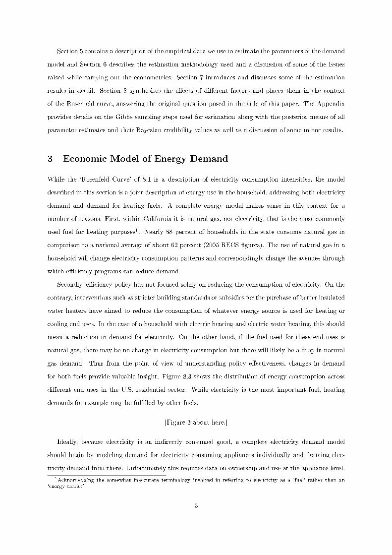
Section 5 contains a description of the empirical data we use to estimate the parameters of the demand

model and Section 6 describes the estimation methodology used and a discussion of some of the issues

raised while carrying out the econometrics. Section 7 introduces and discusses some of the estimation

results in detail. Section 8 synthesises the e�ects of di�erent factors and places them in the context

of the Rosenfeld curve, answering the original question posed in the title of this paper. The Appendix

provides details on the Gibbs sampling steps used for estimation along with the posterior means of all

parameter estimates and their Bayesian credibility values as well as a discussion of some minor results.

3 Economic Model of Energy Demand

While the `Rosenfeld Curve' of 8.1 is a description of electricity consumption intensities, the model

described in this section is a joint description of energy use in the household, addressing both electricity

demand and demand for heating fuels. A complete energy model makes sense in this context for a

number of reasons. First, within California it is natural gas, not electricity, that is the most commonly

used fuel for heating purposes1. Nearly 88 percent of households in the state consume natural gas in

comparison to a national average of about 62 percent (2005 RECS �gures). The use of natural gas in a

household will change electricity consumption patterns and correspondingly change the avenues through

which e�ciency programs can reduce demand.

Secondly, e�ciency policy has not focused solely on reducing the consumption of electricity. On the

contrary, interventions such as stricter building standards or subsidies for the purchase of better insulated

water heaters have aimed to reduce the consumption of whatever energy source is used for heating or

cooling end uses. In the case of a household with electric heating and electric water heating, this should

mean a reduction in demand for electricity. On the other hand, if the fuel used for these end uses is

natural gas, there may be no change in electricity consumption but there will likely be a drop in natural

gas demand. Thus from the point of view of understanding policy e�ectiveness, changes in demand

for both fuels provide valuable insight. Figure 8.3 shows the distribution of energy consumption across

di�erent end uses in the U.S. residential sector. While electricity is the most important fuel, heating

demands for example may be ful�lled by other fuels.

[Figure 3 about here.]

Ideally, because electricity is an indirectly consumed good, a complete electricity demand model

should begin by modeling demand for electricity consuming appliances individually and deriving elec-

tricity demand from there. Unfortunately this requires data on ownership and use at the appliance level,

1Acknowledging the somewhat inaccurate terminology involved in referring to electricity as a `fuel' rather than an`energy carrier'.

3

information which is almost always unavailable to the empirical researcher2.

Consequently, in this paper I derive the demand function from a �exible utility function representing

overall bene�ts from both electricity and the secondary heating fuels3. Households are assumed to

maximize an indirect utility function v(p, I) of the following form

v =

y + ψ [exp(−θePe) + exp(−θhPh)] when secondary fuel consumption occurs

y + ψ [exp(−θePe)] when no secondary fuel is consumed

where y is income, v is total utility and Pe and Ph are the average prices of electricity and the

secondary heating fuels consumed. This model is an expression of the practical fact that most households

cannot be said to exercise much choice in whether or not they have access to natural gas or fuel oil for

heating. Conditional on their choice of a house to live in, it is reasonable to suggest that any further

consumption decisions are based on the fuels available. It is only when heating is provided by natural

gas or fuel oil that consumption decisions must optimize over both electricity and the heating fuel. An

alternative view of this formulation is that this analysis separates the decision to use a secondary fuel,

from the decision on how much to consume. The �rst is implicitly made when a home is chosen while

the second is an ongoing process of utility maximization conditional on the �rst decision.

This functional form for utility has been used in the literature studying demand for telephone minutes

(e.g. Narayanan et al. 25, Hobson and Spady 15). The properties of this utility function have been

discussed in Narayanan et al. 25. It is attractive for my purposes primarily because it lends itself to

an easily estimable and �exible demand function, is suited to applications where income elasticity is

insigni�cant, does not impose constant price elasticities, and is consistent with risk averse agents.

This utility function can be interpreted either as modeling demand of a good without signi�cant

income e�ects or as leading to a demand function where the income e�ect is not separately identi�ed

and is instead combined with the constant term. At least in the United States income elasticities have

generally been found insigni�cant, once we condition on the ownership of a particular set of appliances4.

Additionally it can be argued that it is always di�cult to identify an income e�ect for electricity - in

this or other studies - because demand for electricity is the sum of demand for various appliance end

uses. Since empirical data rarely measures the full appliance stock within a household it is di�cult to

claim that one has controlled for appliance ownership in measuring income elasticities. Without such

2As appliance speci�c monitoring and feedback becomes more common in the short to medium term, this constraint maychange allowing us to understand signi�cantly more than we do now about changes in behaviour in response to variationsin price and other characteristics of energy.

3Heterogeneity implies that households with di�erent appliance stocks are allowed to have di�erent parameters in theutility and demand functions.

4Reiss and White [27]�nd this result using a subset of the data I employ (California RECS 1993,97).Dubin and McFadden[9] and Parti and Parti [26] �nd similar results. Train and Mehrez [31] study the welfare implications of optional Time ofUse pricing of electricity, employing a Gorman polar form utility leading to a demand function free of income e�ects.

4

control, the coe�cient on income in a demand estimation problem also measures the e�ects of increasing

(unobserved) appliance stocks with increasing income. Thus the income elasticity is fundamentally

unidenti�ed, motivating the choice of such a functional form.

It is possible from the indirect utility to derive the demand for electricity and the heating fuel using

Roy's identity so that

xe = −∂v/∂pe∂v/∂y

= ψθp exp(−θpPe) (3.1)

xh = −∂v/∂ph∂v/∂y

= ψθh exp(−θpPe) (3.2)

Here xe, xh represent demand for electricity and the secondary fuel and ψ is a vector of demand

modi�ers. If we let ln(ψ) = βZ+ε ∼ N(0, σ2) where Z is a set of observed modi�ers of demand (including

a constant term), β are parameters in the demand function and ε is an unobserved component, then we

can transform this equation to a log-level demand function of the following form5

ye = ln(xe) = βZ − θpPe + ε (3.3)

The form of the demand function obtained here is quite standard, with one restriction, namely cross

price elasticities that are set to zero. This restriction is reasonable (and often used in the recent literature,

as in [27]) where the barriers to fuel switching are high. This describes the situation for the residential

sector very well, where it is extremely hard and expensive to change heating fuels once the home is

constructed. These end uses make up most of the non-electric energy end uses. Of the remainder, it is

technically possible to swap from gas to electric clothes dryers but this is still expensive, requiring the

purchase of an entirely di�erent appliance. This particular end use is also only a small fraction of overall

energy use (about 0.6 percent in 2006, based on the 2010 Buildings Energy Databook).

4 Econometric Speci�cation

I model households as being heterogeneous in the way in which they use energy and in their responses to

variations in factors such as income, household size, prices or climate variations. An ex-ante segmentation

of households into di�erent types is carried out using a set of observable characteristics. From the

point of view of understanding policy, observable heterogeneity is particularly useful for many reasons.

Predicting the impact of similar measures in a di�erent population and learning something about the

channels through which policies have worked, requires understanding which types of households have

5Note that the termln θ is combined with the intercept in the demand equation

5

been impacted most. In this instance we may reasonably suppose that households will behave di�erently

depending on their appliance holdings and certain other sociological characteristics. This being the case

it is probable that the impact of California's energy e�ciency policies on actual household consumption

would have varied depending on the type of household in question. In part this is because both regulatory

standards and utility programs have a technology component to them that interacts with appliance stocks.

Improving home insulation for instance will change electricity demand for a household with central air

conditioning much more than it will a household that does not use electricity for cooling or heating.

Thus rebates for insulation and retro�ts will di�er in e�ectiveness depending on the type of adopter.

In addition to observable heterogeneity, the model structure allows for unobservable heterogeneity in

the demand parameters associated with each household type. The latter is important because ignoring

unobserved heterogeneity will in general lead to biased parameter estimates and inference (see 1). In

particular, simulations of counterfactuals in a model of household demand may be inaccurate where

unobservable heterogeneity is not modeled but functional forms are non-linear. To the best of my

knowledge this study is the �rst examination of e�ciency policy to explicitly address this problem.

A hierarchical model is therefore used to describe demand. At the top level are the type speci�c

demand equations for electricity and natural gas

xe,t = f(Zt, Pe,t, εe,t;βe,t, θe,t) (4.1)

xh,t = f(Zt, Ph,t, εh,t;βh,t, θh,t) (4.2)

βe,t = Ge,t∆e + νe ∼ N(0, Vek) (4.3)

βh,t = Gh,t∆h + νh ∼ N(0, Vhk) (4.4)

θe,t = Ge,t∆e + ηe ∼ N(0, Vep) (4.5)

θh,t = Gh,t∆h + ηh ∼ N(0, Vhp) (4.6)

~ε = [εe,t εh,t] ∼ N(~0,Σ) (4.7)

Here xe,t, xh,t represent annual consumption vectors of electricity and the secondary (heating) fuel

(in units of KWh and Btu respectively) for all households of type t. f is the demand equation and will

be of the form in Equation 3.3, Zt are a set of demand modi�ers6. Pe,t and Ph,t are vectors of average

prices of electricity and the secondary fuel for households of type t.

The subscript t identi�es demand equations for type t ∈ (1, 2...T ) with non price parameters βe,t and

βh,t respectively. θe,t and θh,t represent the own price coe�cients for electricity or natural gas (these are

not price elasticities since the demand equation is log-linear in consumption and price). The demand for

6These could include climate, demographics, housing unit characteristics, occupancy information and so on.

6

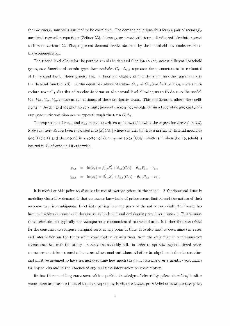
the two energy sources is assumed to be correlated. The demand equations thus form a pair of seemingly

unrelated regression equations (Zellner 33). Thusεe,h are stochastic terms distributed bivariate normal

with some variance Σ. They represent demand shocks observed by the household but unobservable to

the econometrician.

The second level allows for the parameters of the demand function to vary across di�erent household

types, as a function of certain type characteristics Gt. ∆e,h represent the parameters to be estimated

at the second level. Heterogeneity inθe is described slightly di�erently from the other parameters in

the demand function (β). In the equations above therefore Ge,t 6= Ge,t(see Section 6).η, ν are multi-

variate normally distributed stochastic terms at the second level allowing us to �t data to the model.

Vek, Vhk, Vep, Vhp represent the variance of these stochastic terms. This speci�cation allows the coe�-

cients in the demand equation to vary quite generally across households within a type while also capturing

any systematic variation across types through the term Gt∆t.

The expressions for xe,t and xh,t in can be written as follows (following the expression derived in 3.3).

Note that here Zt has been separated into [Z′

t CAt] where the �rst block is a matrix of demand modi�ers

(see Table 1) and the second is a vector of dummy variables (CAt) which is 1 when the household is

located in California and 0 otherwise.

ye,t = ln(xe) = β′

e,tZ′

t + δe,t(CA)− θe,tPe,t + εe,t

yh,t = ln(xh) = β′

h,tZ′

t + δh,t(CA)− θh,tPh,t + εh,t

It is useful at this point to discuss the use of average prices in the model. A fundamental issue in

modeling electricity demand is that consumer knowledge of prices seems limited and the nature of their

response to price ambiguous. Electricity pricing in many parts of the nation, especially California, has

become highly non-linear and demonstrates both 2nd and 3rd degree price discrimination. Furthermore

these schedules are typically not transparently communicated to the end user. It is therefore non-trivial

for the consumer to compute marginal costs at any point in time. It is also hard to determine tier rates,

and information on the times when consumption crosses tiers, from the only regular communication

a consumer has with the utility - namely the monthly bill. In order to optimize against tiered prices

consumers must be assumed to be aware of seasonal variations, all other breakpoints in the tier structure

and must be assumed to have learned over time how much they will consume over a month - accounting

for any shocks and in the absence of any real time information on consumption.

Rather than modeling consumers with a perfect knowledge of electricity prices therefore, it often

seems more accurate to think of them as responding to either a biased price belief or to an average price,

7

and as making decisions under price uncertainty. Borenstein [4] discusses this issue in some detail and

�nds for a population in California that reproducing empirical distributions of consumption seems to

require modeling consumers as either optimizing over the tiered schedule with some error, or reacting

only to the average or marginal price. In earlier work Shin [30] �nds evidence suggesting consumers seem

to respond to average not marginal prices. Most recently Ito [19] uses utility level data to suggest that

in the short run at least, consumers seem to respond to average prices and not marginal prices or the

full tier structure.

This type of evidence would then suggest that models that assume households fully optimize over

the non-linear schedule (see for example Reiss and White 27) are less than ideal descriptions of actual

consumer behaviour, even though they are satisfying in a theoretical sense. In recent years some authors

have chosen alternative formulations of consumer response, either using simpler models of price response

or combining optimization over a tiered schedule with a behavioral `optimization error' term (see McRae

23).

In this paper I incline towards a description of consumer behavior that implies a continuous choice

model with demand being in�uenced by the average price rather than the outcome of solving a discrete

continuous demand problem over the non-linear schedule. This choice seems best suited to a long run

model estimated using annual demand data, and a reasonably good description of actual consumer

behavior at this point in time. That said, this paper is not intended to be a de�nitive statement on how

households respond to electricity price changes. Answering that question requires studying the nature

of household response to non-linear prices under uncertainty and incomplete information.

4.1 Treatment E�ects and the California policy bound

California's history of program interventions aimed at encouraging energy e�ciency may be regarded

as a `treatment' to which households within the state have been exposed. The e�ects of this treatment

will naturally vary across individual households and in most cases cannot be inferred separately for each

unit. For this reason we are often interested in some average e�ect over the whole population. This is

the average treatment e�ect (ATE).

In testing for a California policy e�ect I proceed as follows. In Zt I include a dummy variable that

equals 1 for households in California. Let the coe�cients associated with this dummy in the two demand

equations be δe,t, δh,t ∈ βe,t, βh,t. The magnitude of δt is interpreted as an indication of the type speci�c

e�ect of being in California on a household's energy consumption (either of electricity or the secondary

fuel) over and above di�erences in the structural covariates in Z and prices P . By estimating a type

speci�c e�ect δt I am able to capture heterogeneity in household responses to state and utility programs.

8

This may be regarded as the average di�erence owing to unaccounted factors varying systematically

between California and the rest of the nation. Some of this California e�ect could owe to policy and

regulatory di�erences between the state and nation. δ will approach the true treatment e�ect if one

believes that outcomes in households outside California provide, on average, a valid counterfactual to

which the treated group (the state) can be compared7 for the purpose of policy evaluation.

It is not my intention to claim that the counterfactual formed by households outside California is

a perfect choice. Whether this is so depends on how completely the covariate controls correct for non-

policy di�erences in the two groups. In interpreting δt a more conservative assumption would be that it

represents an approximation to policy impact and possibly an upper bound. At the very least the size

of δ is suggestive as to whether the role of policy has been large or small, and how similar it is to the

occasional estimates produced by regulatory bodies, using di�erent evaluation methods.

It is also worth discussing why I have not included a more explicit indicator of policy e�ort in the

model (as opposed to a state dummy alone). Perhaps the most detailed public information on e�ciency

spending is the utility speci�c expenditure amounts on energy e�ciency measures that are publicly

available from EIA-861 returns archived by the Energy Information Administration. Unfortunately

using utility spending data (available aggregated at state or district level) necessitates a more macro-

level examination of policy impact which in turn removes our ability to ask questions about heterogeneous

impacts across households. Utility expenditure also proxies for only one aspect of policy e�ort in a state

or region and does not relate to many other important measures such as the stringency of building and

appliance standards, the e�ect of state funded public information campaigns and so on8.

Secondly, it is has been argued that the expenditure data publicly available su�er from serious errors

(Horowitz 18) and are consequently unreliable estimates of either policy e�orts or actual spending. To the

extent this is true, including these covariates (even if one were to also include some measure of building

standards of di�ering strictness) would introduce a known and potentially large error into estimates.

Such an error is di�cult to deal with because it is unclear whether the resulting quanti�cation of policy

impacts over-estimates or under-estimates true policy e�ects.

The results of this study suggest it is plausible that at least for this state, e�ciency policy has had

signi�cant impacts but does not by any means tell a complete story (see Section 8). The values of δt

in the population are also consistent with the conclusion that building standards and HVAC appliance

7To be more precise the model undertakes a comparison of households of a speci�c type inside California with theircorresponding types outside the state. That is, the segmentation in the demand function implements a form of matchingwherein similar households are compared to each other in the two populations. This should increase the con�dence wehave in the validity of comparisons.

8This is also a concern in evaluating the results from studies focused on evaluating utility DSM , since regulatorymeasures such as the stringency of building standards (that tend to be correlated with high utility spending) have notgenerally been controlled for in previous work. An exception is the work of Arimura et al. [2] who do include a measureof building standards in their regressions. However that paper �nds no signi�cant e�ect of such standards, perhaps anindication that they are inadequately capturing these regulatory measures using the dummy variables they employ.

9

standards may have made a signi�cant di�erence to energy demand.

4.2 The demand model

Column 1 of Table 1 lists the covariates that enter the two top level demand functions for households

(Z,Pe, Pg), and Columns 2 and 3 specify the variables entering the various segmentation equations at

the second level of the hierarchy.

The second level of the model describes the heterogeneity in parameter estimates in terms of a lower

level vector of type variables. These are all binary variables that take either a 1 or a 0 value for any

given household. For instance a rich household surveyed in 2001, using electric air conditioning, electric

water heating but without any electric heating appliances, luxury goods or durables would have a type

vector as follows: Gt = [1(Intercept), 1, 1, 0, 0, 0, 1(Time)]. A household type t is by de�nition, a group of

households, all of whom have exactly the same group characteristics. These variables are primarily meant

to describe the appliance stock in a household in line with our underlying assumption that households

with di�erent appliances will respond di�erently to incentives, structural factors and policy.

All characteristics in Column 2 of the table enter the vector Ge,t and all except time enter Ge,t

(see Section 6.4.1). The type speci�cation for the heating fuel (Gh,t) is de�ned using a subset of these

characteristics (Intercept, Electric Heating, Low Income and Time). The heterogeneity speci�cation for

the secondary fuel segments households into 32 types corresponding to the 23 combinations that the three

second level variable values can take. Of these 31 are represented in the data. In the electricity demand

model I estimate coe�cients for 97 household types9. Because the groups in the electricity demand

system are more �nely de�ned than the heterogeneity speci�cation for natural gas one may regard all

households as simply belonging to one of 97 types (so that t ∈ [1 . . . 97]). Thus the mapping from an

electricity type to a natural gas type is onto but not one-one (there may be many electricity household

`types' corresponding to the same natural gas `type')

[Table 1 about here.]

5 Data

A major challenge to researchers attempting to evaluate the e�ectiveness of e�ciency policy has been

obtaining suitable empirical data. Most of the existing literature on this question has employed macro

data available at the state or utility level and often at a yearly resolution for the last couple of decades.

Examples include Horowitz 16, Loughran and Kulick 22 and Arimura et al. 2. These studies have all

9After removing a few outliers, some observations with missing data and certain types with less than 15 observationscumulatively over all RECS surveys from 1993 to 2005, I am left with 96 household types actually represented in the data.

10

had as their object, an evaluation of the e�ectiveness of utility expenditure in the United States. With

the exception of Horowitz, the others have generally used EIA data on expenditures as reported.

The analysis in this paper uses the detailed household level microdata available every 4 years through

the Residential Energy Consumption Survey (RECS). The RECS is a cross-sectional survey of house-

holds across the United States, administered by the Energy Information Administration, providing con-

sumption and expenditure data on a variety of energy sources along with details of the physical and

demographic characteristics of the household and the appliance stock possessed. The sample is proba-

bility weighted and the survey has been conducted at four year intervals from 1978 to 2005 (the most

recent available data). The 2005 survey collected data from 4,382 households in housing units statisti-

cally selected to represent the 111.1 million housing units in the United States. The survey is conducted

through in-home interviews and include an inventory of appliances and a survey of the respondent. The

data set is supplemented with consumption �gures from the utility and weather data from the National

Weather Service (NWS). Further details about the RECS data and survey design are available in EIA

[10]. RECS data are tabulated for the four Census regions, the nine Census divisions, and since 1993

for the observations from the four most populous States - California, Florida, New York, and Texas -

are separately identi�ed. In order to identify California observations, I am restricted to using only the

survey data from 1993 and later.

I pool together four RECS surveys from the 1993, 1997, 2001 and 2005 RECS to carry out estimation.

The additional detail in this data set allows me to estimate a more informative structural model than

would be possible relying on aggregate state level data. Combining all four iterations of the RECS

surveys (1993, 1997, 2001, 2005) I have a total of 19,779 observations available for inference, with about

42 percent belonging to the period after 200110. Table 2 provides the observed average values of electricity

consumption (KWh) and secondary heating fuel consumption (1000 BTU) within and outside California.

[Table 2 about here.]

The RECS surveys provide for signi�cant cross-sectional variation in prices, consumption, climate,

demographic characteristics and the other covariates that enter the demand function (see Appendix A).

This variation identi�es the demand system. Note that not all possible household types are represented

in the data used for estimation and some types may be represented only by a few observations. Even

so to the extent the model identi�es variation in parameters at the second level, it can be used to make

inference about 100 percent of the population. For those types with few observations, it is the model

structure at the second level (variation in demand parameters with type characteristics) that is used to

infer demand parameters at the top level. A time dummy is introduced that separates the 1993 and

10This is re�ective of the steadily decreasing sample sizes that the RECS has made available to researchers over the lastfew survey years. The 2009 RECS is expected to use a much larger sample and should help reverse this trend.

11

1997 cohorts from those from the 2001 and 2005 survey years. This enables us to test for changes in the

demand function over time although we are admittedly losing some time variation through combining

two survey years together.

6 Estimation

The model speci�ed in Equations 4.1 through 4.7 is estimated as a Bayesian hierarchical linear model

with the top level consisting of a two equation Seemingly Unrelated Regression Equation (SURE) system.

Posterior distributions of parameters are obtained using a Gibbs sampler. The priors used are proper,

and highly uninformative so that given the number of sample observations, �nal posterior distributions

are essentially insensitive to the prior. Normal distributions are employed for the demand parameters

at the �rst and second level of the model with an inverse Wishart prior for the variances. Appendix

A provides more details of the prior distributions used and the form of the posteriors. I use a burn

in period of 40000 iterations by which time the Markov chain is observed to converge. I then use the

next 10000 draws as samples from the �nal estimated posterior. A brief derivation of the conditional

posterior distributions and the full likelihood, along with the steps of the Gibbs sampler, is provided in

the Appendix. The reader is encouraged to refer to Rossi et al. [29] for a more detailed discussion of the

estimation of Bayesian hierarchical linear models.

6.1 Estimating price elasticities

A challenge to estimation arises from the fact that electricity price schedules have typically been non-

linear, in particular in the last 10-15 years, and even earlier in California. It is common to see utilities

o�er electricity on a tiered price schedule, with marginal prices rising depending on the block in which

consumption is currently taking place. Figure 8.4 illustrates this with a representation of the tiered

pricing schedules currently o�ered by PG&E in California.

[Figure 4 about here.]

The RECS data sets used here, which to the best of this authors knowledge represent the only such

national survey instrument, span the period from 1993 to 2005. The survey provides researchers with

only the average price paid by consumers, not their full rate schedule. Unfortunately, under a tiered rate

structure the average price is no longer exogenous to demand and simply regressing consumption against

price may lead to biased estimates of average price elasticies.

To instrument for endogenous prices, I use two additional variables. First I employ dummies for the

census division. These are exogenous to demand but correlated with price to a limited degree, capturing

12

variations in generation and transmission costs and regulatory fees across the country. Next, for the 1993

and 1997 survey years I obtain the local utility average price for baseline quantities of electricity and

natural gas for each household11. This price is exogenous to the household demand equation because

it is not a�ected by consumption levels, and is predetermined by utilities in consultation with the

regulator (typically over a three year period). It is therefore also uncorrelated with individual, annual

shocks. Thus it ful�ls the so called exclusion restriction. At the same time, the predetermined baseline

price is correlated with average prices because a signi�cant amount of the inframarginal consumption

of households is billed at a rate identical or close to the exogenous utility area rate (even though the

marginal unit may be billed at a slightly higher or lower tier).

Instrumental variable methods in bayesian models are still a relatively new addition to the literature.

This paper implements the method described in Yang et al. [32], to augment the demand side equations

described above with a limited information supply side model for average price, using the two instruments

just described. In brief (see Appendix for more), the demand system described in Equations 4.1-4.7 is

augmented with a supply side speci�cation for price as described below. Here IVe,hare the instruments

for electricity and the secondary heating fuel, namely census division dummies and the exogenous utility

area rate12. Note that the supply side speci�cation also allows for heterogeneity in that the degree

of correlation between instruments and the the average price is allowed to be di�erent across the 31

di�erent natural gas household types. While dropping or adding this �exibility does not change our �nal

estimates much, we frame the model this way because an examination of utility pricing structures reveals

that tiered rates do in fact di�er between (for example) all-electric households and dual fuel households.

pe,t = αe,tIVe,t + ωe,t

ph,t = αh,tIVh,t + ωh,t

αe,t = GhSe,t + νe ∼ N(0,Whk)

αh,t = GhSh,t + νh ∼ N(0,Whk)

Et = [εe,t, εh,t, ωe,t, ωh,t] = N(0, S) (6.1)

The relationship between demand side prices and the supply side is captured by linking the stochastic

terms in the demand equation and the pricing equation, as in Equation 6.1.

11This variable was originally released as part of the survey microdata and has since been removed. I managed to obtainthe original survey data sets containing the two exogenous price variables. Thanks for this are owed to Peter Reiss. Forthe 2001 and 2005 surveys this variable was not available and has not been released by the EIA.

12For the heating fuels in some cases more than one fuel type is consumed (for examples small amounts of propane alongwith the major heating fuel). The instrument (and the average price on the left hand side) is a weighted average of theindividual fuel prices in those cases.

13

The complete model can now be estimated using a simple Markov Chain Monte Carlo sampler, with

one addition complication. Going back to the discussion of instruments a few paragraphs ago, one of the

problems we have to overcome is that instruments are available only for about half the sample (the 1993

and 1997 survey years). With one additional assumption this constraint is straightforward to circumvent

in a bayesian paradigm. The assumption we make is that the type speci�c, price response coe�cient

does not change over time. Appliance stocks are still allowed to modify the price coe�cient and thus

the primary source of heterogeneity is still retained. Referring back to remarks made in Section 4, it is

for this reason that the second level heterogeneity speci�cation for electricity is di�erent from the other

parameters in that the Time variable is not present in Ge,t (see Table 1 and equations 4.1-4.7).

With this assumption in place, the complete estimation is carried out using a two stage procedure.

First, I use only the �rst half of the dataset and instrumenting for price, recover type speci�c price

coe�cient posteriors (along with those for the other parameters). Next in step two I re-estimate the

demand side using the complete dataset. In this step I treat the price coe�cient as known and where

required in the MCMC sampler, I draw from the posterior estimated in step one. Since the �rst step

yields a consistent estimate of the price coe�cients for all types, this distribution may be used in the

second stage provided we are willing to treat the price coe�cient as a structural parameter that does

not change signi�cantly between the 1993-1997 period and the 2001-2005 period.

As I show in Section 7.2, it turns out that the price elasticity I estimate is very close to prior estimates

in the literature that have used the full price schedule and have been estimated for similar households.

7 Results

I discuss the results emerging from the estimated demand system in three parts. I begin in Section 7.1

with an overview of the extent to which California households seem to di�er from their counterparts

elsewhere, once we control for a variety of structural factors. I show this amount is relatively small -

certainly when compared to the stark picture the Rosenfeld curve presents on its own. Next in Section

7.2, I consider the issue of price response and the variation in this parameter within the population. In

doing so I also discuss the average elasticity I estimate in the context of other results in the literature. In

Section 7.3 I discuss evidence that emerges from this model and the RECS data that supports theories of

the existence of split incentive market failures that reduce the adoption of e�ciency measures in rented

homes.

The model estimated here provides us information on the observable and unobservable heterogeneity

in demand parameters associated with other factors beyond price and the state dummy. Table 3 provides

estimates of all second level parameters for electricity and the secondary heating fuel. The columns of

14

the table correspond to parameters in the demand function and rows correspond to characteristics of

type (as present in Ge,h). The estimates at the second level tell us how the presence or absence of a

group characteristic modi�es the parameters of demand. The values provided are means of the posterior

distributions at the second level with signi�cant values marked with a star. The last row of the table

provides the scale of the demand function covariates. Finally, note that these estimates can be related

to percentage changes in energy consumption owing to di�erent type characteristics.

Interpreting this table requires some care. The row headers are characteristics that a household

might possess and segment the population into di�erent types. Each of these characteristics are binary

as described in Section 4.2. The column headers are variables in the demand function. The numbers

within the cells can be used to read o� the coe�cients of the estimated demand function. An example

might be helpful. Consider Row 1 (Base Row). This row provides the estimated demand function for

households that have none of the appliance stocks/ characteristics that are listed below. They have no

electric air-conditioning, no electric heating, are not low income and so on. For these households, the

demand function coe�cients corresponding to each of the demand modi�ers (Intercept, HDD, CDD and

so on) can be read o� in the cells directly to the right. The price coe�cient of -2.35 indicates a negative

price elasticity (approximately -0.235 at 10 cents per KWh). The coe�cient -0.13 (corresponding to the

California dummy δ) indicates that this type of household consumes about 13 percent less electricity in

California than elsewhere.

The rows below the Base row tell us how demand needs to be modi�ed as household characteristics

change. For example, the addition of electric air-conditioning alone will change the demand function for

a household and the nature of the new demand function is obtained by adding together the Base Row

and the Electric Air-Conditioning row (Row 2). Thus for instance the intercept will go up by from 7.94

to 8.44 (a change of 0.50), as one would expect since an additional electrical end use is now present.

Sensitivity to heating degree days changes dramatically from an insigni�cant estimate of 0.09, to a highly

signi�cant estimate of -0.26. Again this makes sense because an appliance is now present whose use is

strongly in�uenced by temperature. In a similar vein the California dummy coe�cient decreases further,

from -0.13 to -0.22 (a decrease of -0.09). This indicates that the gap between CA and non-CA homes

widens when we consider households with air-conditioning as well.

[Table 3 about here.]

7.1 The role of policy

The primary purpose of estimating this model is to understand how much of a di�erence remains between

California households and others in the nation, once we account for the various structural parameters

15

in the demand function. This is represented by the state dummy for CA (denoted by δe,h). Each of the

household types represented in the population is allowed to have a di�erent value of δt and it is evidently

interesting to see how δt varies across types because this tells us something about which policies may

have been most e�ective.

Note that it is possible that there are spillover e�ects associated with at least some of California's

e�ciency policies. Accounting for spillovers rigorously is di�cult at the best of times, but it is reasonable

to argue that for program interventions centered around mandatory building standards and incentives

provided to residential consumers to make e�ciency purposes, any spillovers are likely to be limited.

Assuming very signi�cant spillovers would seem to go against observed consumer reluctance to invest in

energy e�ciency - the energy e�ciency gap is a puzzling and di�cult problem precisely because much of

the time consumers do not seem to rationally undertake energy saving behavior. That said, regardless of

ones beliefs as to the magnitude of these considerations, it would still be accurate to regard the 'policy

e�ect' estimated here as a net e�ect, over and above any spillovers. From the point of view of explaining

the Rosenfeld curve (which also only measures net di�erences between state and nation) we need only

explain this net e�ect.

The estimated parameter values δt are interesting and suggest a limited in�uence of policy. The values

of δ may be expressed in terms of a percentage reduction in electricity or heating fuel use associated with

being in California owing to the e�ect of e�ciency measures and any confounding unobservables missing

in the model. When combined with the representation of household types in the population (using the

probability weights associated with each observation in the RECS survey) they can be used to obtain a

distribution of residual e�ects (δ)13. Figures 8.5 and 8.6 illustrate these distributions for electricity and

the secondary heating fuels respectively.

Note that each of these �gures contains two distribution plots - one computed using the distribution

of households in the United States as a whole and the other using the California distribution. Because

the distribution of household types in the two populations is not identical, and because the reductions

captured by δ vary with type, we would expect the nature of demand shifts in the country as a whole to

di�er from that in California even if both groups had been subjected to exactly the same policy measures

and reacted in similar ways. The di�erences between the distribution shapes and mean reductions in

Figures 8.5 and 8.6 illustrate this fact. They also demonstrate how the estimates of a model can be used

to make predictive statements about another population and why heterogeneity is so important here. It

is precisely because all households are not the same, and will not react to a program intervention the

13As a rough approximation the parameter value directly translates to a percentage decline but to determine percentagesaccurately it is necessary to also account for the fact that each type speci�c δt estimate is associated with a householdtype with di�erent mean consumption levels. Furthermore posterior distributions of δt di�er across types. To accuratelycompute expected population distributions therefore, one needs to carry out a simulation exercise using the posteriorparameter distribution.

16

same way, that the results of similar interventions in di�erent populations will di�er. For that reason,

simply calculating an average estimate of policy impact is only of limited utility.

The �gures show the simulated distribution of treatment e�ects (the `California E�ect' captured by

δ). There is heterogeneity induced by the di�erent household types in the population, each of which

are allowed to have a di�erent average e�ect. The curve is smooth because the model �ts a normal

distribution to each of the di�erent types, what is plotted is therefore a mixture of normals. The table

shows how δ varies across types and is simple the relevant column taken from Table 3.

Overall the estimates of δ capture an e�ect corresponding to around a 13.7 percent reduction in

California (as a percentage of the national average consumption). For the secondary heating fuel (natural

gas for the most part in California), the California e�ect unexplained by structure is much higher at about

40 percent of the national average. At �rst glance this might suggest that there are confounding factors

in the secondary fuel demand model that are contributing to this di�erence. Two potential confounds of

this type are household behavior and technology di�erences. However while both may contribute to the

overall e�ects captured by δ it is not entirely misleading to regard them as indicators of `e�ciency'.

With regards behavior - especially as it relates to heating end uses - the RECS data sets do reveal

some evidence of di�erences in the way Californians treat energy when compared with the rest of the

nation. For instance in 2005, more Californians reported lowering the temperature in the day when the

house is empty and while sleeping than the national average. As many as 45 percent of Californian

residents reported that they switched o� heating when the house was empty as opposed to about 8

percent for the nation as a whole. There are two points of view that one might take regarding such

conservation behavior. One is that it represents the outcome of regulatory and utility e�orts to educate

consumers about the importance of saving energy. The other point of view is that Californians are

intrinsically di�erent from the rest of the nation and these di�erences arise completely independent of

policy. As with all things, the truth probably lies somewhere in between, but this author inclines more

to the former point of view.

The other cause for a large di�erence, especially in natural gas consumption, may be intrinsic tech-

nological di�erences. In grouping together the secondary heating fuels because of their similarity in how

the consumer interacts with them we have also compared di�erent combustion technologies. Natural gas

home heating tends to be more e�cient than using fuel oil where the need to maintain exhaust at a cer-

tain minimum heat results in combustion e�ciencies that normally cannot exceed 85 percent. A natural

gas furnace on the other hand, which burns a higher quality fuel, can be much more e�cient (around 95

percent for the best models). Unfortunately I am unaware of any good estimate of the e�ciency of the

stock of home furnaces in di�erent parts of the country and therefore it is hard to separate the role of

this factor in explaining δh.

17

7.1.1 Have HVAC interventions been the real success story?

Figures 8.5 and 8.6 also provide the estimated parameter values for δe, δh at the second level of the

hierarchy (as does Table 3). This is useful to see how the di�erence between households in the state and

those outside varies depending on type characteristics. These estimates provide a type of di�erence in

di�erences estimator that suggests that heating and cooling end uses might be one area where program

interventions have been especially successful.

[Figure 5 about here.]

[Figure 6 about here.]

The tables next to the distribution plots tell us how the di�erence between CA and non-CA house

varies with the presence of type characteristics. The �rst row (Base) is the magnitude of δe associated

with households that have none of the additional electrical end uses - that is no electric heating, water

heating or cooling, a zero for the durables indicator. They are also not in the poorest quintile and do

not own homes. The parameter value in the second row (Electric AC for Figure 8.5) indicates that

households with this characteristic show an even larger CA e�ect (δ values going from -0.13 for Base

types to −0.22, an addition of −0.09, when an electric AC is owned). The rows below this tell us

whether this di�erence increases or decreases as a speci�c type characteristic is `added on' (that is they

provide the net e�ect of each characteristic on δe). There are signi�cant e�ects associated with electric

air-conditioning, electric heating, durables ownership and time. The di�erence also increases on average

with time (about 7 percent between the 1993-97 and the 2001-2005 cohorts). Finally - and somewhat

counter-intuitively - the state nation divergence reduces when the durables indicator is 1. Low income

households also show a greater than average California e�ect.

These numbers are interesting, especially those associated with the electric air conditioning and

heating dummies, because in one sense they provide stronger evidence of the role of policy than the

top level distribution of δealone. Recall that one disadvantage of the estimate δe is that it potentially

contains other factors that are unobserved but correlated with California households and independent

of e�ciency policy. The change in δe in households with electric air-conditioning however might do a

much better job of eliminating unobserved confounding factors. To be speci�c, one may assume that

the base value of δe (about 13 percent) captures any confounding e�ects and some fraction of e�ciency

policy impacts that in�uence even `base' consumption households. Then the increment to δe owing to

electric air conditioning (a further 9 percent reduction) exists over and above these confounds (it is

the di�erence in δe values between households with and without electric air-conditioning) and provides

much stronger evidence that policy interventions may have helped reduce energy used for cooling end

18

uses. This is indicative of a signi�cant impact of building standards, insulation rebates, air-conditioner

appliance standards and so on.

A similar argument holds for the increased (in magnitude) state e�ect (δ) for households with electric

heating and this again points to possibly large impacts of programs targeting HVAC technologies. These

measures include Title 24 building standards, rebates provided for the purchase of insulation and for

home retro�ts and utility �nanced installation of programmable thermostats in homes. Finally, other

programs that are not focused on heating and cooling (such as e�cient CFL lighting subsidies) may have

played some role in driving the baseline reduction that is observed. Other recent work that has suggested

a signi�cant impact of building standards in California is Kahn and Costa [20] and Aroonruengsawat

et al. [3].

The change in δe corresponding to Time in the second level points to a diverging trend. This estimator

measures the di�erence in rates of change between the two populations. Whether this owes to greater

policy di�erences in this period or not is debatable. However it is consistent with the implication of the

Rosenfeld curve that the state of California has steadily pulled away from the nation over time. The

estimate is small but highly signi�cant even though only a limited amount of time variation is available

in the data. Note that over the period of time studied here the rate of divergence between the two

population intensities does seem to have slowed.

Lastly we have a result that suggests that households in California with more durables (or at least

both a clothes washer and a clothes dryer) are signi�cantly less di�erent in percentage terms than their

counterparts elsewhere (there is signi�cant positive increment in δe). This might suggest that households

in California with more durables consume more electricity without an o�setting di�erence in e�ciency

compared to their counterparts elsewhere.

7.2 Price response

While the central objective of this study is not to estimate price elasticities, the price coe�cients esti-

mated over the household types are still of some interest. One reason for this is that prices of electricity

and natural gas are signi�cantly in�uenced by regulatory policy. In California, utility decoupling initia-

tives and utility driven e�ciency programs have certainly in�uenced the rate structures consumers see.

The average prices of electricity in California are not a result purely of market forces, indeed there would

be a strong case for arguing that the largest single determinant of rate changes is regulatory policy. In

any case to the extent prices may be slightly di�erent between the state and the rest of the nation,

overall consumption should be expected to be di�erent as well. The degree to which price variations will

in�uence electricity and secondary fuel consumption levels will depend on the price response (inferred

19

from parameters θe,h) that is suggested by the data. Note that the parameters θe,h do not directly

translate to price elasticities but can be expressed as such (εe = θePe). Also, as with the parameter in

the previous section we need to draw from type speci�c elasticity posteriors to obtain the distribution in

population of the price elasticity.

Figure 8.7 presents the type speci�c electricity price elasticities implied by the model corresponding

to an average price of 10 cents per KWh (2005 dollars). I interpret my price response as being closer

to the medium to long run elasticity of demand which is likely to be larger than a short run elasticity.

Whether these are reasonable estimates is a di�cult question to answer because it is hard to �nd much

agreement in the literature on what the medium term price elasticity of residential electricity demand

actually is. Previous work has estimated widely divergent elasticities. In a meta survey Espey and Espey

[12] found that the literature contains estimates of short run price elasticities ranging between -2.01 to

-0.004 with a mean of -0.35. Long run elasticities range between -2.25 to -0.04 with a mean of -0.85

and a median of -0.81. Similarly Reiss and White [27] discuss the range of price elasticity estimates in

the literature and suggest that numbers ranging from nearly 0 to -0.6 are most commonly obtained. In

recent work using a California speci�c data set, Gillingham et al. [14] �nd a price responsiveness of near

0 for the speci�c end use of electric heating. The price elasticities infered here seem reasonable in this

light.

There is one interesting feature of the distribution of elasticity estimates that is worth noting. For a

population distribution of household types that matches California, there seems to exist a multimodal

distribution of price responsiveness with a long tail. There is a large probability mass of less responsive

consumers with elasticities around -0.40 and lower and then another cluster of consumers with elasticities

around -0.6 (at a constant price). As a qualitative matter, my results indicate that the distribution of

price elasticities in California is di�erent from that in the rest of the country with a larger mass of less

responsive consumers. This owes to the distribution of di�erent household types with heterogeneous

price response coe�cients.

[Figure 7 about here.]

Figure 8.7 also contains a table showing how the price coe�cient varies with type characteristics. In

general there is evidence that consumers with more electrical end uses are more responsive to price -

consistent with the idea that they have more `room to manouvere' since they have a greater number of

appliances whose use can be adjusted14.

I also obtain price elasticities for the secondary heating fuel (primarily fuel oil and natural gas)

14Households using more electricity are probably paying higher bills and consequently may be more aware of the e�ectsof price changes. This would also lead to similar results of greater elasticities for heavy users but it is not clear that in across sectional study of annual elasticities this type of individual salience argument is meaningful.

20

corresponding to a price of 100 cents per therm. Figure 8.8 presents these estimates. In general price

responsiveness seems higher than in the case of electricity and the distribution of heterogeneity in the

population is much smoother.

[Figure 8 about here.]

7.3 The `Split Incentives' problem

It has often been theorized in the energy literature that home owners may be more likely than renters

and/or households that do not pay for electricity directly, to make energy e�ciency investments (see

Murtishaw and Sathaye 24). This is an instance of an incentive compatibility problem wherein households

who do not own their dwelling are unlikely to be willing to make long term investments with large capital

costs that would improve the energy e�ciency of the building. At the same time the owner might not

wish to make this investment either energy bills are paid by the tenant and consequently there would be

no direct bene�t to the owner from making e�ciency upgrades.

As a consequence one might expect energy consumption in dwellings occupied by owners to be lower

than it is in rented homes. In practice however, this hypothesis has been di�cult to test directly. Two

recent working papers that attempt to shed some light on this problem are Gillingham et al. [14] and

Davis [8]. The authors come to mixed conclusions. The �rst paper looks at heating energy use and �nds

no strong evidence of di�erences in energy consumption, nor the temperature levels at which thermostats

are set. The authors do point out however that households show certain di�erences in the frequency

with which they change heating and cooling temperature settings depending on whether they pay for

heating or not. They also point out that insulation levels seems better in households which own their

dwelling. Davis examines whether there is a signi�cant di�erence in the ownership of energy e�cient

appliances between home owners and tenants (based on the 2005 RECS data) and �nds that there is does

seem to be the case. This paper does not look at di�erences in other investments such as insulation and

weatherization however, both of which (as the author also notes), might be even more likely candidate

for split incentive problems. Unfortunately neither of these two studies looks at energy use directly.

I am able to make a contribution to this debate and highlight some of the reasons why it may be

di�cult to detect split incentive considerations in practice. To do this we need to look at the way the

constant term in the demand function changes for the two fuel types (electricity and the secondary fuel),

depending on whether or not the household owns the dwelling. This information is provided in Table 3

in the �rst column.

21

7.3.1 Electricity versus the secondary fuel

To begin, let us consider the di�erence between the qualitative sign of the parameter estimates associated

with home ownership for the two fuels. Electricity use seems to increase for households that are home

owners. The parameter estimate at the second level is 0.43 and signi�cant, translating to an increase in

electricity consumption of about 48 percent associated with home ownership15. This likely re�ects two

factors at play here. First, home owners, all else equal are likely to be richer than those who are renters.

While the income e�ects associated with electricity consumption may be small, appliance ownership

(as I have remarked earlier) will increase with income. To the extent that home ownership plays the

part of a proxy for greater income and increased appliance stocks, it is unsurprising that electricity use

may increase for home owners. Secondly, even at the same income level, it is likely that home owners

may make greater investments in electricity using appliances than renters. `Feathering ones nest' is an

important part of living in your own house and one might expect home owners to invest in a variety of

small and large appliances - home theatre systems, increased lighting, workshop equipment in garages

and so on.

If home owners do indeed gradually accumulate more electricial appliances it is not surprising that

their net electricity consumption will exceed that of renters. This e�ect may well swamp any e�ciency

improvements that might occur because of increased adoption of e�ciency enhancing technologies. I

suggest this underlies the increase in electricity consumption levels predicted for electricity by the model.

Detecting split incentives in electricity consumption might therefore be much easier to do by looking

directly at the existence of e�cient appliances in the home (rather than overall electricity consumption).

This is the approach Davis [8] takes.

The situation is somewhat di�erent for secondary heating fuels - natural gas, fuel oil and the like.

Unlike in the case of electricity, it is by no means clear that increases in income would translate to the

addition of di�erent end uses for these fuels. This is simply a re�ection of the fact that these fuels are

primarily used for thermal heating purposes, which tend to be limited to cooking, space heating, water

heating and occasionally clothes drying. Furthermore whether or not a household is set up to use natural

gas for these end uses is primarily a consequence of the availability of the fuel and building construction

considerations that are not easily amenable to changes after the initial choice. Thus income increases

would not necessarily translate to a wider range of end uses for the secondary fuel. This is all the more

so since the end uses for the secondary fuels are rather basic and would need to be in place whether or

not the resident owns or rents the dwelling.

15This number can be calculated by converting the log parameter estimates to original energy consumption numbers (bytaking an exponent of the parameter value). For electricity, mean consumption by renters is given by eEr where Eris thelog of average electricity consumption by renter households. The increase in expected consumption due to a switch to homeownership is given by e(Er+∆i) − eEr , where ∆i is the parameter estimate corresponding to home-ownership (0.43).

22

As a consequence of these di�erences in the way electricity is used as opposed to the secondary fuels,

one might expect that di�erences in the level of investment in e�ciency enhancing technologies would

more visibly in�uence energy consumption of heating fuels than it would electricity.Recall that large

capital intensive investments with long pay back periods - retro�ts, insulation upgrades and the like - are

all strong candidates for split incentive problems and at the same time are aimed largely at improving

HVAC e�ciency. And indeed, in the case of the heating fuels, the demand model predicts entirely

di�erent behavior for homeowners as opposed to renters. The coe�cient estimate is again signi�cant but

negative implying a decrease in secondary fuel consumption of about 29 percent corresponding to a shift

from a rented dwelling to an owned dwelling.

I therefore interpret the signi�cant negative coe�cient associated with home ownership (indicative of

signi�cant declines in consumption of heating fuels for such homes) as being relatively strong evidence

that is consistent with the existence of incentive compatibility market failures. Taken together with

the results in Davis [8], which focused on electricity and suggested that home owners may possess

more e�cient appliances on average, I suggest that these results present evidence that the split incentive

problem may be even more severe for the other fuels. Table 4 presents some other, more direct, indicators

of energy e�ciency investments focusing on behaviors that are closely tied to the end uses that the

secondary fuels are used to ful�ll. The intent is simply to show that there seems consistent evidence

of increased di�usion of these technologies and behaviors amongst home owners than renters (who may

not pay utility bills directly and may have fewer incentives to invest in home e�ciency upgrades). This

might explain why they appear to consume less energy. For a more rigorous claim one would wish to

control for other covariates such as income and credit constraints and the like in comparing the outcome

variables in Table 4, but that is an analysis best left to a separate study.

[Table 4 about here.]

8 Synthesis

It is helpful to collect together the model estimates for both electricity and the secondary fuel in order

to break down the Rosenfeld e�ect into its constitutive components. I use the demand parameters

estimated here for di�erent household types and combine these with RECS sample weights to obtain

implied reductions in California demand due to various structural factors. Similarly, I also form a

population estimate for the California dummy (or bound on treatment) δe,h.

The Rosenfeld curve is normally drawn in units of per capita electricity consumption and energy

per capita is a very commonly used statistic when discussing how the energy use characteristics of pop-

ulations. Therefore Figures 8.9, 8.10 use this metric and convert household reductions to per capita

23

reductions. In order to compute these e�ects sizes the estimated demand function parameters are com-

bined with California and non-California mean values for the various covariates. This is done separately

for each household type and averaged over the population using the RECS sampling weights correspond-

ing to each type. This tells us the in�uence of the structural di�erences between California and the

United States. I plot reductions due to only those factors that pass a signi�cance test - i.e for whom

the uncertainty in demand parameter posteriors is not so large as to negate the possibility of making

statistically signi�cant statements regarding the di�erence between the two populations. For instance,

ye,t = ln(xe) = β′

e,tZ′

t + δe,t(CA)− θe,tPe,t + εe,t

∆KWHt,price = exp(θe,tPCA,t + Eca)− exp(θe,tPUS,t + Eca,t)

∆KWHprice is an estimate of the change in annual electricity consumption that a household type in

California would show if prices faced by all members of that type were changed to be the same as those

outside the state (all else held equal). When PCA,t (the actual California prices) is systematically higher

than PUS,t (prices in non-CA households) then ∆KWHprice will be negative, implying a reduction in state

consumption owing to higher prices. Here θe,t is the price coe�cient estimated from the data and Eca,t is

the mean electricity consumption in California for the type in question. Because the parameter estimates

θe,t are stochastic with some estimated posterior distribution the implied change in consumption will

also be uncertain. The distribution of ∆KWHprice can be used to carry out a signi�cance test. Note

that the primary e�ect of climate is likely to be in changing the type distribution (determined largely

by appliance ownership) of households. For instance household types with electric AC are less common

inside California. This is in part a climate e�ect but will in�uence energy consumption independent of

any e�ciency program e�ects. The block marked type distribution in the graphs below accounts for these

di�erences in population composition. Consequently I interpret the HDD and CDD e�ect as representing

additional e�ects on demand over and above their in�uence on appliance purchase.

[Figure 9 about here.]

[Figure 10 about here.]

It is easy to see from Figure 8.9 that the average reductions in electricity consumption that we

may attribute to non-price policy impact is very limited at about 317 KWh per capita annually or

approximately 20 percent of the overall di�erence between the state and the rest of the nation. This is

still a signi�cant reduction of course but it suggests a very di�erent story than a comparison of electricity

24

intensities by themselves. When the impact of price is included the total share due to price (heavily

in�uenced by regulation) and policy is about 512 KWh annually or 32.5 percent of the actual di�erence.

The recently released California Energy Commissions 2010-2020 Demand Forecast model provides

updated o�cial estimates of cumulative savings in the residential sector over time. A comparison with

California Energy Commission (CEC) estimates of the e�ects of utility programs and regulatory stan-

dards is instructive. It is a di�cult task to accurately quantify savings gained from these e�orts, in

large part because of the variety and number of individual utility programs. The CEC does produce

some aggregate �gures, compiled from the aggregation of various quanti�cation methodologies applied

to individual programs, the outputs from a detailed energy system model, and self reported utility esti-

mates of savings16. Education, training and awareness generation programs are excluded from savings

estimates due to the di�culty in quantifying them. Some caution should be exercised in interpreting

CEC estimates provided for comparison in Table 5 because numbers published in di�erent years as part

of the demand forecast models have typically been subject to changes and modi�cations. The �gures

reported here are the total electricity savings estimates for 2001 and 2005 from the California Energy

Demand 2010 - 2020 Commission-Adopted Forecast (CEC 2010), which contains revised estimates of

e�ciency savings. It is interesting that the residential sector savings estimates are close to the results

we obtain given that they derive from an entirely di�erent bottom up approach.

[Table 5 about here.]

The relative agreement between the regulator's newest �gures and our own is heartening as an eval-

uation of the California Energy Commission's current methods although as remarked earlier regulator

estimates have been modi�ed on an ongoing basis. That said, it is important and useful to use empirical

microdata as an evaluation technique because in general regulators and a utility do have an incentive to

over-report savings once policy is funded.

I use the econometric model to estimate the policy bound and impact of prices for the 1993-97 and

2001-05 periods and then interpolate between the two periods. I compare with the newest CEC estimates

of program impacts over this period of time. Figure 8.11 contains the results. This graph is instructive

on the question of how much of the Rosenfeld e�ect might actually be policy driven.

[Figure 11 about here.]

For the secondary heating fuel (natural gas in California) I obtain a much larger estimate of δg

suggesting that about 43 percent of the di�erence between California and non-California households

might owe to the state's e�ciency related e�orts. An additional 12.3 percent can be attributed to price

16Some details on the methodology used in making forecasts and savings estimates are available in the Energy DemandForecast Methods Report (California Energy Commission 2005).

25

di�erences and 21.2 percent of the gap owes to di�erences in household types. Again these �ndings

are qualitatively consistent with the conclusions of separate studies carried out recently such as Kahn

and Costa [20] that indicate that building standards might have been an especially e�ective part of the

portfolio of e�ciency enhancing interventions attempted in California.

A few �nal remarks are worth making here. Even though for California it appears that the in�uence

of e�ciency interventions may have been limited in scope, as Figure 8.5 and 8.6 show the impact on

di�erent household types is quite varied. Households with energy expenditures on heating and cooling

end uses seem to be most clearly impacted. Yet with regards electricity demand these types are also only

a relatively small fraction (especially in the case of air conditioning) of the California population. This

would seem to suggest that the potential impact of similar policies - such as strong building standards

and incentives to improve air-conditioner e�ciency - might be much greater in geographies that have

more extreme climates.

To make a broader methodological point, in the energy community, comparisons of energy intensity

are very popular. This single metric (typically expressed per unit GDP instead of per capita) also remains

fundamental to international climate change negotiations. Part of the motivation for this analysis has

been to make the point that while indices such as energy intensities (and more sophisticated versions

derived from decomposition methods) can provide a great deal of insight, they also hide as much as

they reveal. In particular, we need to be careful when we identify seemingly spectacular success stories

screened on the basis of a single aggregate statistic.

References

[1] Greg Allenby and Peter Rossi. Marketing models of consumer heterogeneity. Journal of Economet-

rics, 89(1-2):57�78, November 1998. ISSN 03044076. doi: 10.1016/S0304-4076(98)00055-4. URL

http://linkinghub.elsevier.com/retrieve/pii/S0304407698000554.

[2] Toshi Arimura, Richard Newell, and Karen Palmer. Cost-E�ectiveness of Electricity Energy Ef-

�ciency Programs. Technical report, Resources for the Future, Washington D.C., 2009. URL

www.rff.org/documents/RFF-DP-09-48.pdf.

[3] A. Aroonruengsawat, Maximillian Au�hammer, and Alan Sanstad. The Impact of State Level

Building Codes on Residential Electricity Consumption. Technical report, University of California,

Berkeley, 2009.

[4] Severin Borenstein. To What Electricity Price Do Consumers Respond? Residen-

26

tial Demand Elasticity Under Increasing-Block Pricing. Technical report, 2009. URL

http://econ-www.mit.edu/files/4031.

[5] California Energy Commission. Energy Demand Forecast Methods Report. Report CEC-400-2005-

036, California Energy Commission, June 2005.

[6] California Energy Commission. California Energy Demand 2010-2020: Sta� Energy Demand Fore-

cast. Technical report, California Energy Commission, 2010.

[7] Dan Charles. Energy e�ciency. Leaping the e�ciency gap. Science (New York, N.Y.),

325(5942):804�11, August 2009. ISSN 1095-9203. doi: 10.1126/science.325_804. URL

http://www.ncbi.nlm.nih.gov/pubmed/19679783.

[8] Lucas Davis. Evaluating the Slow Adoption of Energy E�cient Investments: Are Renters Less

Likely to Have Energy E�cient Appliances? Technical report, University of California, Berkeley,

Berkeley, 2010. URL http://ei.haas.berkeley.edu/pdf/working_papers/WP205.pdf.

[9] J. Dubin and D. McFadden. An Econometric Analysis of Residential Appliance Holdings and

Consumption. Econometrica, 52:345�362, 1984.

[10] EIA. Sample Design for the Residential Energy Consumption Survey. Technical report, Energy

Information Administration (US DOE), 1994.

[11] Jiyong Eom and James Sweeney. Shareholder Incentives for Utility Delivered Energy E�-

ciency Programs in California. Technical report, Stanford University, Stanford, 2009. URL

http://ssrn.com/abstract=1401529.

[12] James A. Espey and Molly Espey. Turning on the Lights: A Meta-Analysis of Residential Electricity

Demand Elasticities. Journal of Agricultural and Applied Economics, 36(1):65�81, 2004.

[13] Kenneth Gillingham, Richard Newell, and Karen Palmer. Energy E�ciency Policies: A

Retrospective Examination. Annual Review of Environment and Resources, 31(1):161�192,

November 2006. ISSN 1543-5938. doi: 10.1146/annurev.energy.31.020105.100157. URL

http://arjournals.annualreviews.org/doi/abs/10.1146/annurev.energy.31.020105.100157.

[14] Kenneth Gillingham, Matthew Harding, and Dave Rapson. Split

Incentives in Household Energy Consumption. 2010. URL

http://www.stanford.edu/�mch/GillinghamHardingRapson_SplitIncentives.pdf.

[15] M. Hobson and R.H. Spady. The demand for local telephone service under optional local measured

service. Technical report, Bellcore Technical Memorandum TM-ARH-011423 Summer, 1988.

27

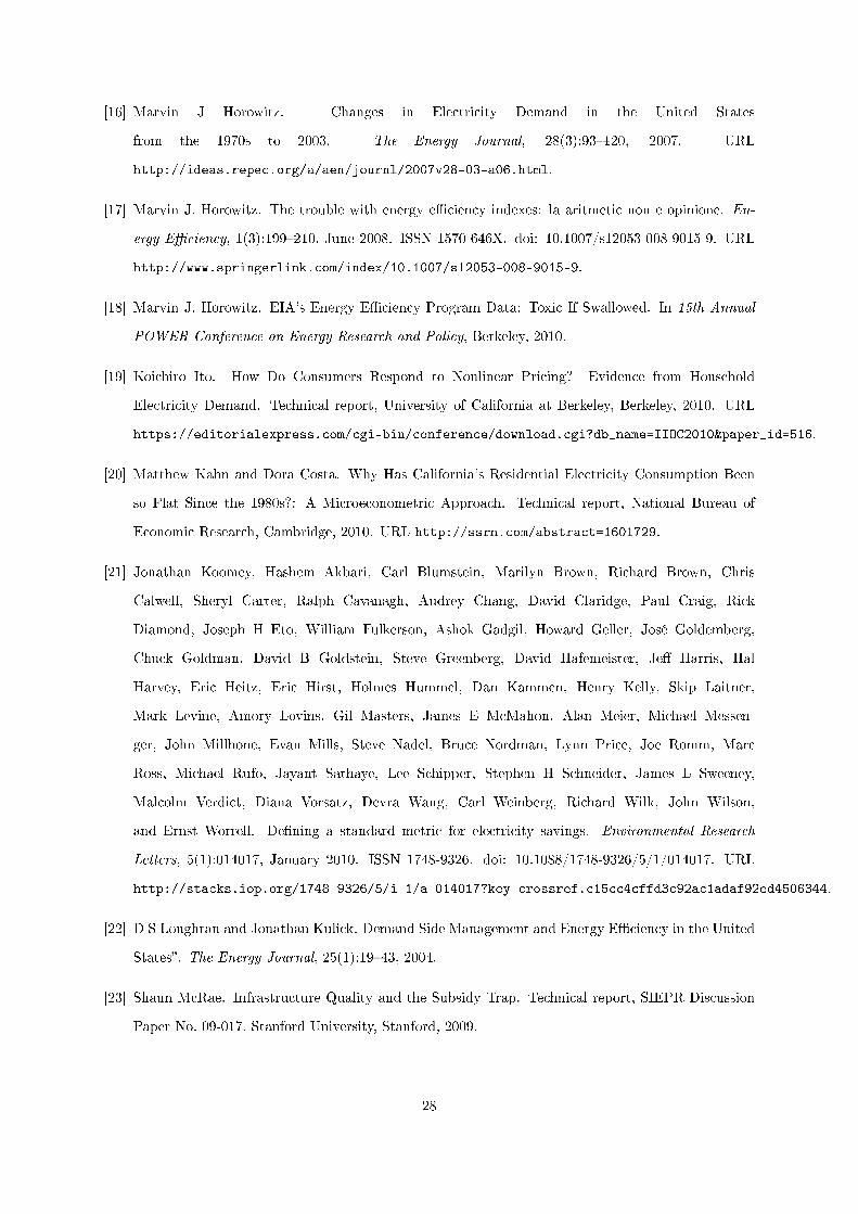
[16] Marvin J Horowitz. Changes in Electricity Demand in the United States

from the 1970s to 2003. The Energy Journal, 28(3):93�120, 2007. URL

http://ideas.repec.org/a/aen/journl/2007v28-03-a06.html.

[17] Marvin J. Horowitz. The trouble with energy e�ciency indexes: la aritmetic non e opinione. En-

ergy E�ciency, 1(3):199�210, June 2008. ISSN 1570-646X. doi: 10.1007/s12053-008-9015-9. URL

http://www.springerlink.com/index/10.1007/s12053-008-9015-9.

[18] Marvin J. Horowitz. EIA's Energy E�ciency Program Data: Toxic If Swallowed. In 15th Annual

POWER Conference on Energy Research and Policy, Berkeley, 2010.

[19] Koichiro Ito. How Do Consumers Respond to Nonlinear Pricing? Evidence from Household

Electricity Demand. Technical report, University of California at Berkeley, Berkeley, 2010. URL

https://editorialexpress.com/cgi-bin/conference/download.cgi?db_name=IIOC2010&paper_id=516.

[20] Matthew Kahn and Dora Costa. Why Has California's Residential Electricity Consumption Been

so Flat Since the 1980s?: A Microeconometric Approach. Technical report, National Bureau of

Economic Research, Cambridge, 2010. URL http://ssrn.com/abstract=1601729.

[21] Jonathan Koomey, Hashem Akbari, Carl Blumstein, Marilyn Brown, Richard Brown, Chris

Calwell, Sheryl Carter, Ralph Cavanagh, Audrey Chang, David Claridge, Paul Craig, Rick

Diamond, Joseph H Eto, William Fulkerson, Ashok Gadgil, Howard Geller, José Goldemberg,

Chuck Goldman, David B Goldstein, Steve Greenberg, David Hafemeister, Je� Harris, Hal

Harvey, Eric Heitz, Eric Hirst, Holmes Hummel, Dan Kammen, Henry Kelly, Skip Laitner,

Mark Levine, Amory Lovins, Gil Masters, James E McMahon, Alan Meier, Michael Messen-

ger, John Millhone, Evan Mills, Steve Nadel, Bruce Nordman, Lynn Price, Joe Romm, Marc

Ross, Michael Rufo, Jayant Sathaye, Lee Schipper, Stephen H Schneider, James L Sweeney,

Malcolm Verdict, Diana Vorsatz, Devra Wang, Carl Weinberg, Richard Wilk, John Wilson,

and Ernst Worrell. De�ning a standard metric for electricity savings. Environmental Research

Letters, 5(1):014017, January 2010. ISSN 1748-9326. doi: 10.1088/1748-9326/5/1/014017. URL

http://stacks.iop.org/1748-9326/5/i=1/a=014017?key=crossref.c15cc4cffd3c92ac1adaf92ed4506344.

[22] D S Loughran and Jonathan Kulick. Demand Side Management and Energy E�ciency in the United

States�. The Energy Journal, 25(1):19�43, 2004.

[23] Shaun McRae. Infrastructure Quality and the Subsidy Trap. Technical report, SIEPR Discussion

Paper No. 09-017, Stanford University, Stanford, 2009.

28

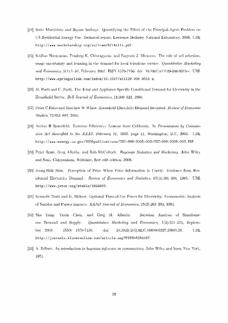
[24] Scott Murtishaw and Jayant Sathaye. Quantifying the E�ect of the Principal-Agent Problem on

US Residential Energy Use. Technical report, Lawrence Berkeley National Laboratory, 2006. URL

http://www.escholarship.org/uc/item/6f14t11t.pdf.

[25] Sridhar Narayanan, Pradeep K. Chintagunta, and Eugenio J. Miravete. The role of self selection,

usage uncertainty and learning in the demand for local telephone service. Quantitative Marketing

and Economics, 5(1):1�34, February 2007. ISSN 1570-7156. doi: 10.1007/s11129-006-9015-z. URL

http://www.springerlink.com/index/10.1007/s11129-006-9015-z.

[26] M. Parti and C. Parti. The Total and Appliance-Speci�c Conditional Demand for Electricity in the

Household Sector. Bell Journal of Economics, 11:309�321, 1980.

[27] Peter C Reiss and MatthewWWhite. Household Electricity Demand Revisited. Review of Economic

Studies, 72:853�883, 2005.

[28] Arthur H Rosenfeld. Extreme E�ciency: Lessons from California. In Presentation by Commis-

sion Art Rosenfeld to the AAAS, February 21, 2005, page 11, Washington, D.C, 2005. URL

http://www.energy.ca.gov/2005publications/CEC-999-2005-003/CEC-999-2005-003.PDF.

[29] Peter Rossi, Greg Allenby, and Rob McCulloch. Bayesian Statistics and Marketing. John Wiley

and Sons, Chippenham, Wiltshire, �rst edit edition, 2006.

[30] Jeong-Shik Shin. Perception of Price When Price Information Is Costly: Evidence from Res-

idential Electricity Demand. Review of Economics and Statistics, 67(4):591�598, 1985. URL

http://www.jstor.org/stable/1924803.

[31] Kenneth Train and G. Mehrez. Optional Time-of-Use Prices for Electricity: Econometric Analysis

of Surplus and Pareto Impacts. RAND Journal of Economics, 25(2):263�283, 1994.

[32] Sha Yang, Yuxin Chen, and Greg M. Allenby. Bayesian Analysis of Simultane-

ous Demand and Supply. Quantitative Marketing and Economics, 1(3):251�275, Septem-

ber 2003. ISSN 1570-7156. doi: 10.1023/B:QMEC.0000003327.55605.26. URL

http://journals.kluweronline.com/article.asp?PIPS=5254167.

[33] A. Zellner. An introduction to bayesian inference in econometrics. John Wiley and Sons, New York,

1971.

29

6000

8000

10000

12000

14000

KW

h p

er

cap

ita

0

2000

4000

6000

1960 1962 1964 1966 1968 1970 1972 1974 1976 1978 1980 1982 1984 1986 1988 1990 1992 1994 1996 1998 2000 2002 2004

KW

h p

er

cap

ita

California United States

Figure 8.1: The Rosenfeld Curve showing the evolution of per capita electricity consumption in Californiaand the United States

30

2000

2500

3000

3500

4000

4500

5000

KW

h p

er

cap

ita

0

500

1000

1500

2000

1960 1962 1964 1966 1968 1970 1972 1974 1976 1978 1980 1982 1984 1986 1988 1990 1992 1994 1996 1998 2000 2002 2004

KW

h p

er

cap

ita

California Residential California Commercial California Industrial

US Residential US Commercial US Industrial

Figure 8.2: Sector-wise comparison of California and US electricity consumption (Source: EIA electricitysales �gures).

31

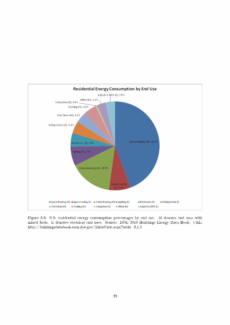
Figure 8.3: U.S. residential energy consumption percentages by end use. M denotes end uses withmixed fuels. E denotes electrical end uses. Source: DOE 2010 Buildings Energy Data Book. URL:http://buildingsdatabook.eren.doe.gov/TableView.aspx?table=2.1.5

32

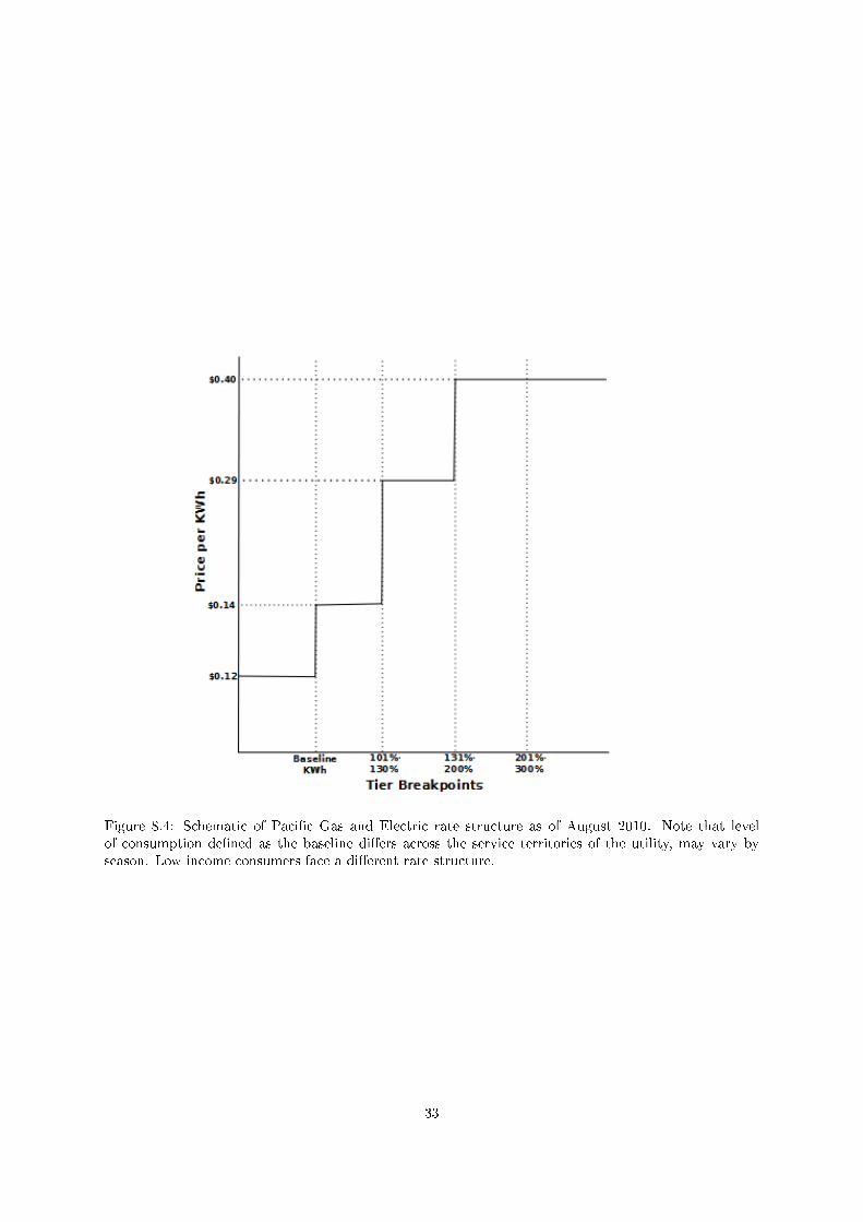
Figure 8.4: Schematic of Paci�c Gas and Electric rate structure as of August 2010. Note that levelof consumption de�ned as the baseline di�ers across the service territories of the utility, may vary byseason. Low income consumers face a di�erent rate structure.

33

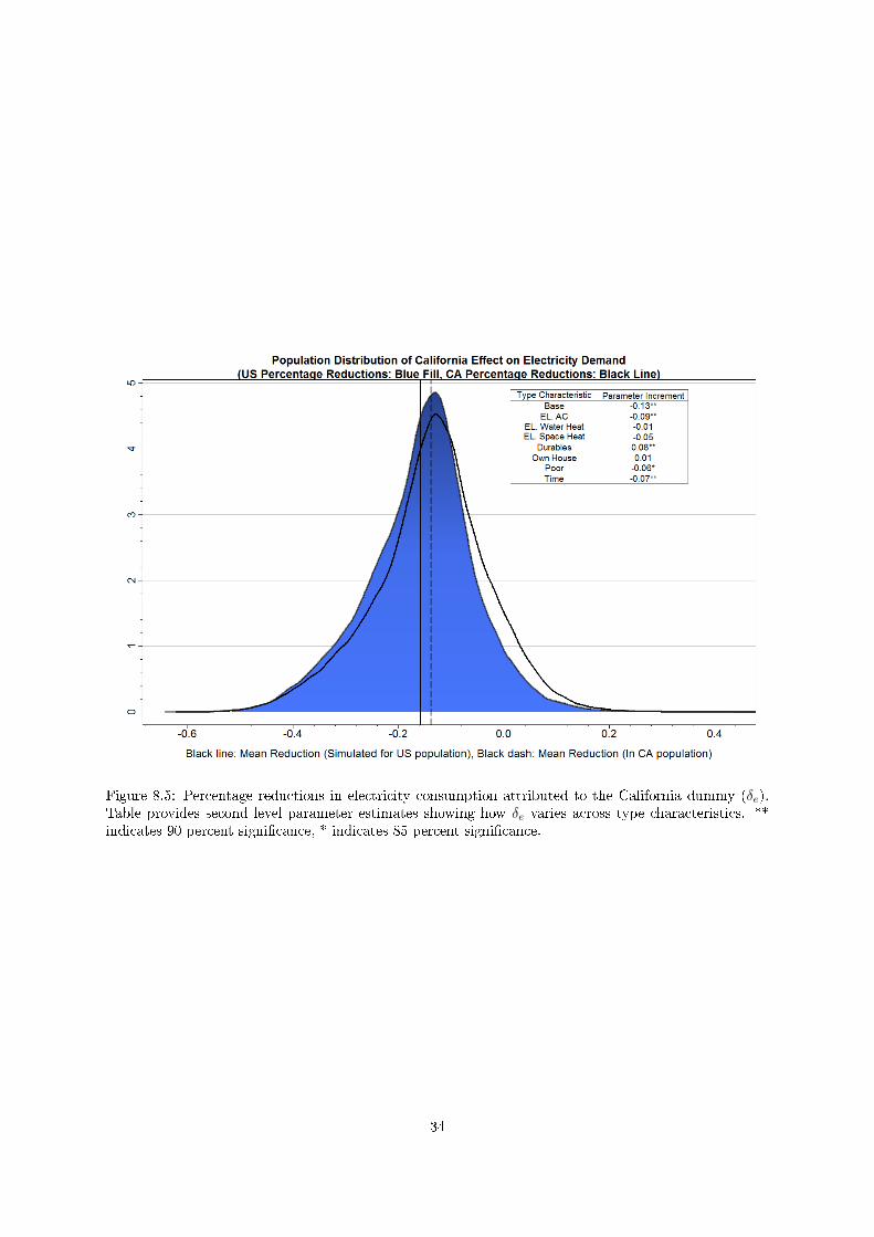
Figure 8.5: Percentage reductions in electricity consumption attributed to the California dummy (δe).Table provides second level parameter estimates showing how δe varies across type characteristics. **indicates 90 percent signi�cance, * indicates 85 percent signi�cance.

34

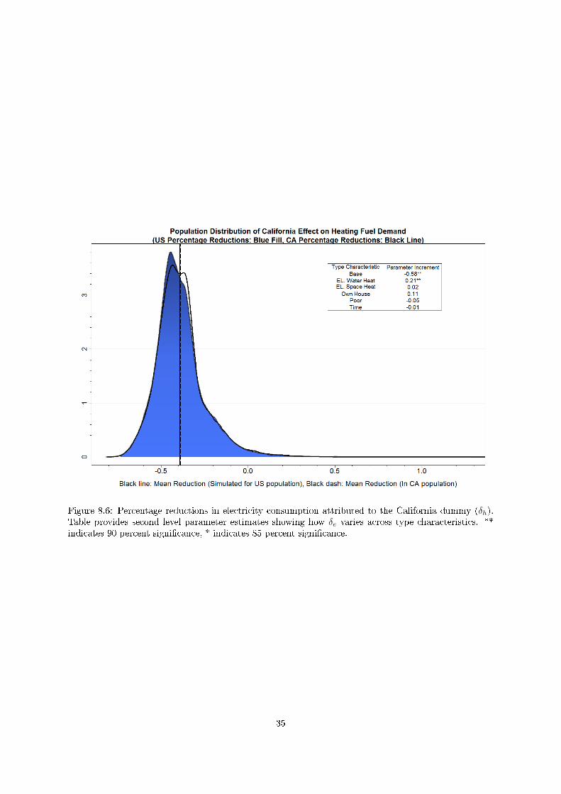
Figure 8.6: Percentage reductions in electricity consumption attributed to the California dummy (δh).Table provides second level parameter estimates showing how δe varies across type characteristics. **indicates 90 percent signi�cance, * indicates 85 percent signi�cance.

35

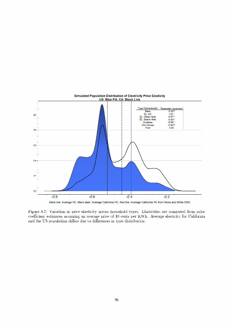
Figure 8.7: Variation in price elasticity across household types. Elasticities are computed from pricecoe�cient estimates assuming an average price of 10 cents per KWh. Average elasticity for Californiaand the US population di�ers due to di�erences in type distribution.

36

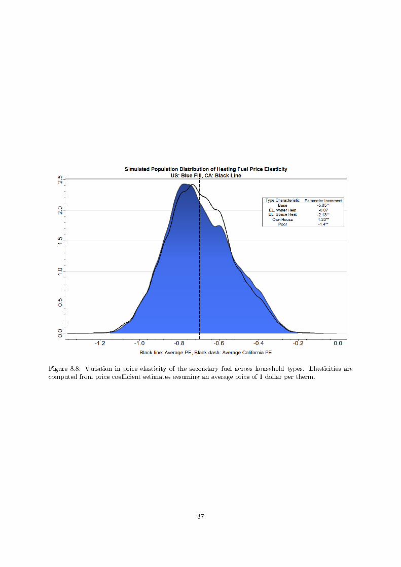
Figure 8.8: Variation in price elasticity of the secondary fuel across household types. Elasticities arecomputed from price coe�cient estimates assuming an average price of 1 dollar per therm.

37

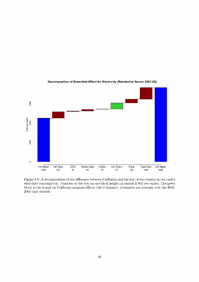
Figure 8.9: A decomposition of the di�erence between California and the rest of the country in per capitaelectricity consumption. Numbers at the bottom are block heights in annual KWh per capita. The greenblock is the bound on California program e�ects (the δ dummy). Estimates are averages over the 2001,2005 time periods.

38

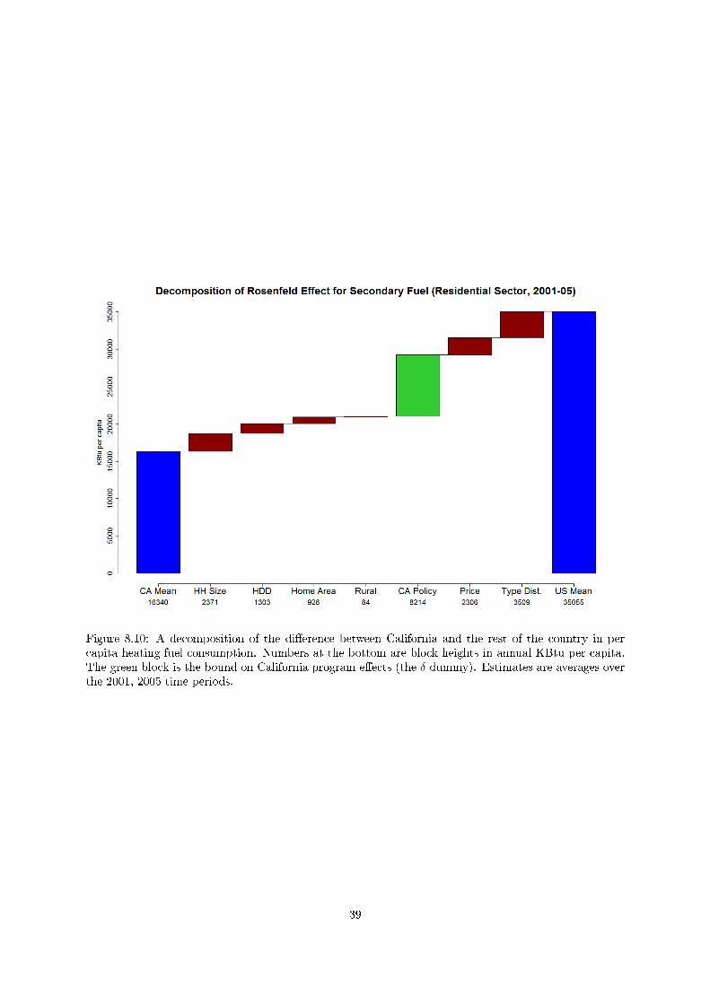
Figure 8.10: A decomposition of the di�erence between California and the rest of the country in percapita heating fuel consumption. Numbers at the bottom are block heights in annual KBtu per capita.The green block is the bound on California program e�ects (the δ dummy). Estimates are averages overthe 2001, 2005 time periods.

39

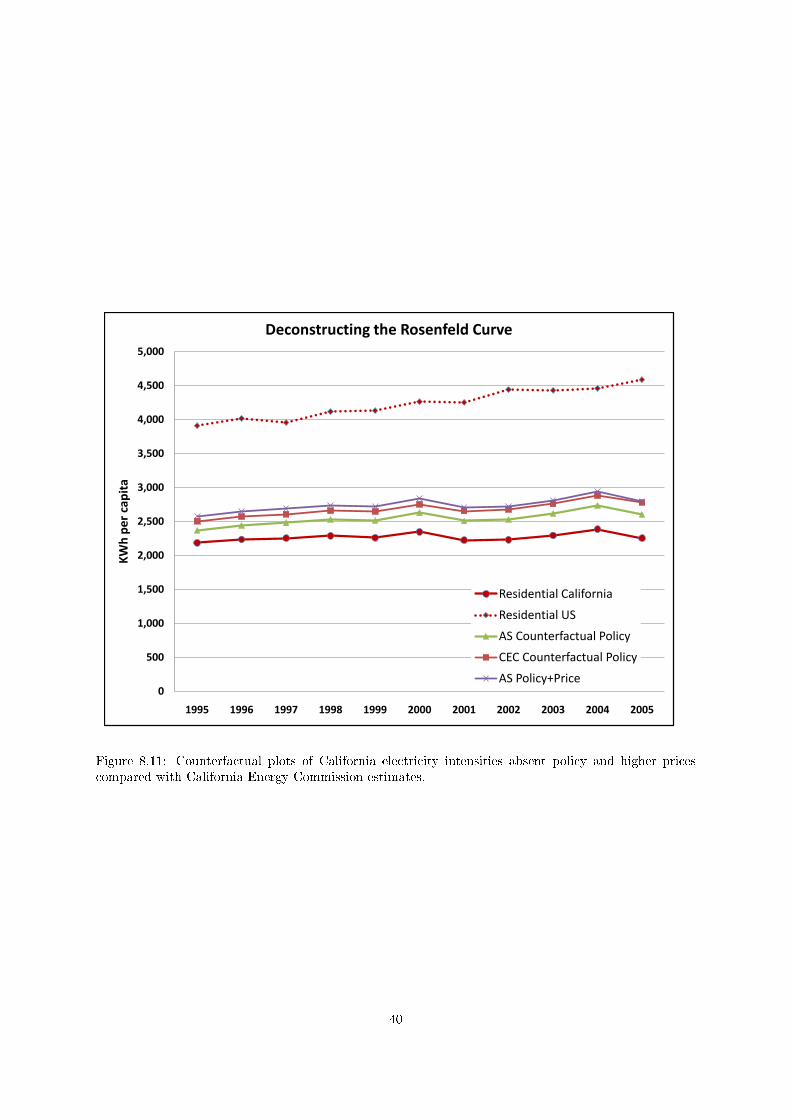
0

500

1,000

1,500

2,000

2,500

3,000

3,500

4,000

4,500

5,000

1995 1996 1997 1998 1999 2000 2001 2002 2003 2004 2005

KW

h p

er

cap

ita

Deconstructing the Rosenfeld Curve

Residential California

Residential US

AS Counterfactual Policy

CEC Counterfactual Policy

AS Policy+Price

Figure 8.11: Counterfactual plots of California electricity intensities absent policy and higher pricescompared with California Energy Commission estimates.

40

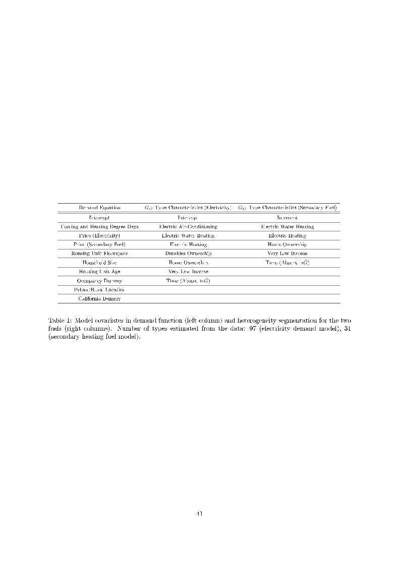
Demand Equation Ge: Type Characteristics (Electricity) Gh: Type Characteristics (Secondary Fuel)

Intercept Intercept Intercept

Cooling and Heating Degree Days Electric Air-Conditioning Electric Water Heating

Price (Electricity) Electric Water Heating Electric Heating

Price (Secondary Fuel) Electric Heating Home Ownership

Housing Unit Floorspace Durables Ownership Very Low Income

Household Size Home Ownership Time (Absent inG)

Housing Unit Age Very Low Income

Occupancy Dummy Time (Absent inG)

Urban/Rural Location

California Dummy

Table 1: Model covariates in demand function (left column) and heterogeneity segmentation for the twofuels (right columns). Number of types estimated from the data: 97 (electricity demand model), 31(secondary heating fuel model).

41

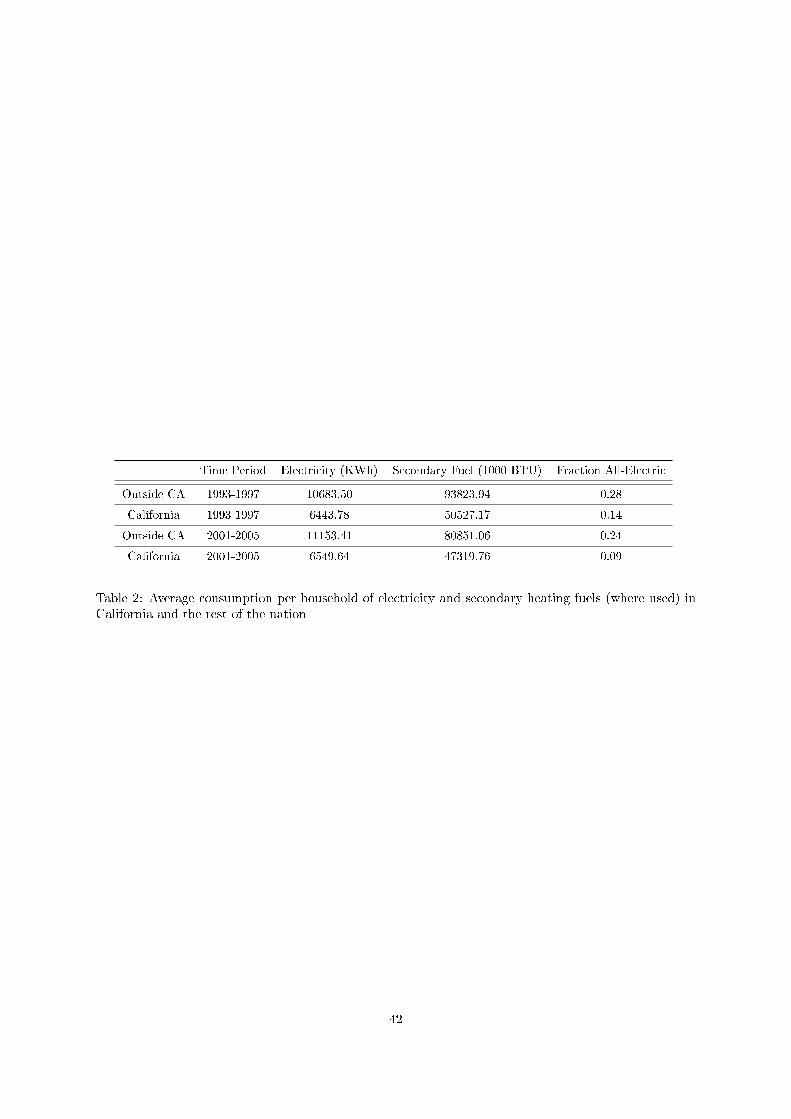
Time Period Electricity (KWh) Secondary Fuel (1000 BTU) Fraction All-Electric

Outside CA 1993-1997 10683.50 93823.94 0.28

California 1993-1997 6443.78 50527.17 0.14

Outside CA 2001-2005 11153.41 80851.06 0.24

California 2001-2005 6549.64 47319.76 0.09

Table 2: Average consumption per household of electricity and secondary heating fuels (where used) inCalifornia and the rest of the nation

42

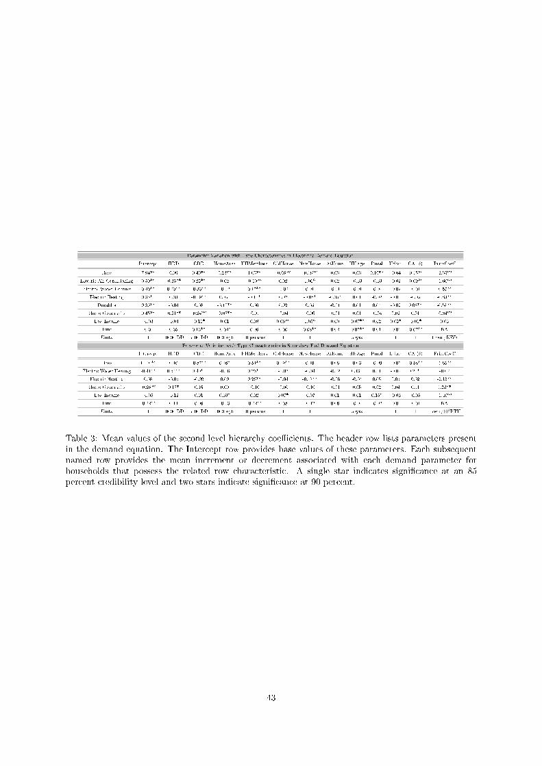
Parameter Variation with Type Characteristics in Electricity Demand Equation

Intercept HDD CDD HomeArea HHMembers OldHouse NewHouse AtHome HHAge Rural Urban CA (δ) PriceCoe�

Base 7.94** 0.09 0.40** 0.23** 1.05** -0.06** -0.16** 0.03 0.03 0.10** -0.04 -0.13** -2.35**

Electric Air-Conditioning 0.50** -0.35** 0.25** 0.02 -0.10** 0.02 0.06* 0.02 -0.03 -0.03 -0.02 -0.09** -1.60**

Electric Water Heating 0.46** 0.20** -0.33** -0.02 0.17** -0.02 0.01 -0.01 -0.01 -0.04 -0.02 -0.01 -0.57**

Electric Heating 0.35** 0.03 -0.19** 0.05* -0.11* 0.02 -0.06* -0.05* 0.01 -0.02 -0.01 -0.05 -0.83**

Durables 0.39** -0.04 0.08 -0.10** 0.06 0.02 0.05 -0.01 0.01 0.04 -0.02 0.08** -0.58**

Home Ownership 0.43** -0.21** -0.24** -0.08** -0.01 -0.04 -0.06 -0.01 0.01 -0.04 0.02 0.01 -0.84**

Low Income -0.03 -0.04 -0.11* 0.01 0.08 0.06** 0.05* 0.00 -0.07** 0.02 0.05* -0.06* 0.03

Time -0.01 0.05 0.13** -0.04* 0.06 0.00 0.08** 0.02 -0.07** 0.01 -0.01 -0.07** NA

Units 1 10000 DD 5000 DD 1000 sq.ft 10 persons 1 1 1 50yrs 1 1 1 1 cent/KWh

Parameter Variation with Type Characteristics in Secondary Fuel Demand Equation

Intercept HDD CDD HomeArea HHMembers OldHouse NewHouse AtHome HHAge Rural Urban CA (δ) PriceCoe�

Base 11.40** 0.16 -0.87** 0.16* 0.54** 0.19** 0.10 0.08 0.03 -0.09 -0.05 -0.58** -5.85**

Electric Water Heating -0.41** 0.54** 0.40** -0.06 0.23** -0.02 -0.04 -0.02 0.13* 0.11 -0.02 0.21** -0.07

Electric Heating 0.08 -0.05 -0.09 0.09 0.26** -0.04 -0.17** -0.06 -0.04 0.05 0.05 0.02 -2.13**

Home Ownership -0.26** 0.18* 0.16 0.00 -0.10 -0.06 -0.10 -0.01 0.05 0.02 0.04 0.11 1.23**

Low Income -0.05 -0.12 0.01 0.03* 0.02 0.07* -0.07 0.01 0.01 0.15* -0.03 -0.05 -1.40**

Time -0.22** 0.14 0.06 -0.03 -0.22** 0.08 -0.12 0.06 -0.04 -0.02 -0.01 -0.01 NA

Units 1 10000 DD 5000 DD 1000 sq.ft 10 persons 1 1 1 50yrs 1 1 1 1 cent/104BTU

Table 3: Mean values of the second level hierarchy coe�cients. The header row lists parameters presentin the demand equation. The Intercept row provides base values of these parameters. Each subsequentnamed row provides the mean increment or decrement associated with each demand parameter forhouseholds that possess the related row characteristic. A single star indicates signi�cance at an 85percent credibility level and two stars indicate signi�cance at 90 percent.

43

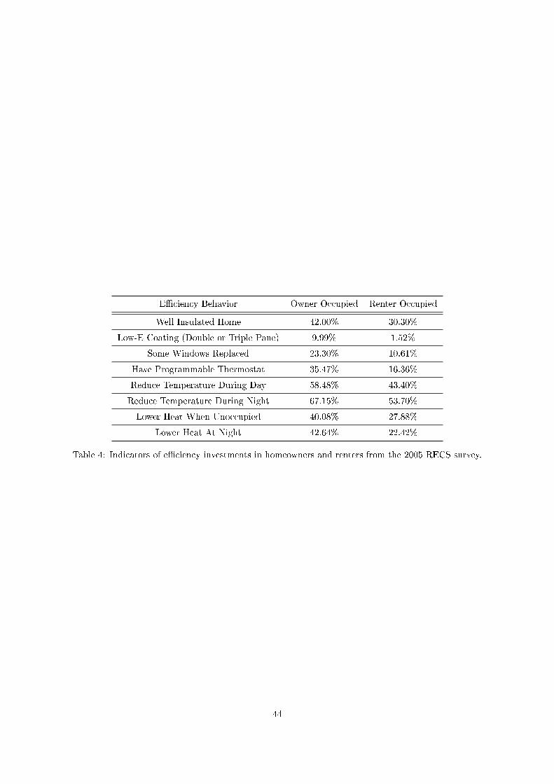
E�ciency Behavior Owner Occupied Renter Occupied

Well Insulated Home 42.00% 30.30%

Low-E Coating (Double or Triple Pane) 9.99% 1.52%

Some Windows Replaced 23.30% 10.61%

Have Programmable Thermostat 35.47% 16.36%

Reduce Temperature During Day 58.48% 43.40%

Reduce Temperature During Night 67.15% 53.70%

Lower Heat When Unoccupied 40.08% 27.88%

Lower Heat At Night 42.64% 22.42%

Table 4: Indicators of e�ciency investments in homeowners and renters from the 2005 RECS survey.

44

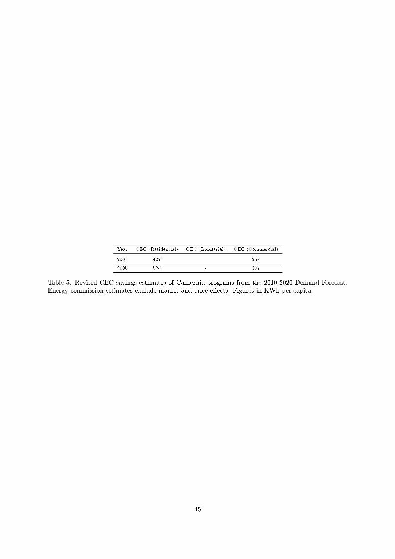
Year CEC (Residential) CEC (Industrial) CEC (Commercial)

2001 427 - 258

2005 524 - 307

Table 5: Revised CEC savings estimates of California programs from the 2010-2020 Demand Forecast.Energy commission estimates exclude market and price e�ects. Figures in KWh per capita.

45