Decomposition of one-dimensional waveformusing iterative Gaussian diffusive

filtering methods

BY YIH-NEN JENG1,*, P. G. HUANG

2AND YOU-CHI CHENG

1

1Department of Aeronautics and Astronautics, National Cheng KungUniversity, Tainan 70101, Taiwan, Republic of China

2Department of Mechanical and Materials Engineering, Wright StateUniversity, Dayton, OH 45435, USA

The Gaussian smoothing method is shown to have a wide transition zone around the cut-off frequency selected to filter a given dataset. We proposed two iterative Gaussiansmoothing methods to tighten the transition zone: one being approximately diffusive andthe other being strictly diffusive. The first version smoothes repeatedly the remaininghigh-frequency parts and the second version requires an additional step to furthersmooth the resulting smoothed response in each of the smoothing operation. Based onthe choice of the criterion for accuracy, the smoothing factor and the number ofiterations are derived for an infinite data length in both methods. By contrast, for afinite-length data string, results of the interior points (sufficiently away from the twoendpoints) obtained by both methods can be shown to exhibit an approximate diffusiveproperty. The upper bound of the distance affected by the error propagation inward dueto the lack of data beyond the two ends is numerically estimated. Numerical experimentsalso show that results of employing the iterative Gaussian smoothing method are almostthe same as those obtained by the strict diffusive version, except that the errorpropagation distance induced by the latter is slightly deeper than that of the former. Theproposed method has been successfully applied to decompose the wave formation of anumber of test cases including two sets of real experimental data.

Keywords: iterative Gaussian smoothing method; diffusive filter on time domain;time-series data

*A

RecAcc

1. Introduction

The least-squares method is widely used in many mathematical, physical andengineering applications (Marr & Hildreth 1980; Lancaster & Salkauskas 1986;Jeng 2000; Fasshauer 2002; Liew et al. 2002). When the dataset to be analysed iscomplicated, a lower degree polynomial approximation is not sufficient tocapture the profile trends and a high-degree polynomial is frequently suggested.However, a high-degree polynomial approximation is more complicated toimplement and it can sometimes give rise to undesirable oscillations.

Proc. R. Soc. A

doi:10.1098/rspa.2007.0031

Published online

uthor for correspondence (z6208016@email.ncku.edu.tw).

eived 15 May 2007epted 15 February 2008 1 This journal is q 2008 The Royal Society

Y.-N. Jeng et al.2

If the least-squares method is defined locally at every point, the method iscalled the moving least-squares method (Lancaster & Salkauskas 1986). Themethod can be applied in both discrete and continuous datasets, but in this workwe shall consider only the former cases. Moreover, the moving least-squaresmethods can be used in conjunction with a weighting kernel of Gaussianexponential function to eliminate unnecessary spurious oscillation (Marr &Hildreth 1980; Mackworth & Mokhtarian 1984; Mokhtarian & Mackworth 1986;Lowe 1989; Weiss 1994; Jeng 2000; Fasshauer 2002; Liew et al. 2002; Jeng &Cheng 2004). If the approximated polynomial is of the zeroth degree, the methodbecomes the conventional Gaussian smoothing method (Mackworth &Mokhtarian 1984; Mokhtarian & Mackworth 1986; Lowe 1989). Among manyavailable weighting kernels for the zeroth-order moving least-squares method,the Gaussian exponential function has the following two useful properties.First, by a careful selection of an appropriate smoothing factor, s, as definedin the Gaussian function exp [Kx2/(2s2)], there exists a desired threshold fre-quency above which the waveforms can be effectively filtered out. Second,the relation between the original data and resulting smoothed data is akin tothat observed between the initial temperature distribution and the exactsolution at a corresponding instant of the equation for unsteady one-dimensionalheat conduction (Carslaw & Jaeger 1957). In other words, the Gaussiansmoothing method is closely related to the spontaneous diffusion process ofnature and therefore obeys the second law of thermodynamics (Morse &Feshbach 1953).

The signal decomposition using the wavelet transform has been successfullyapplied to many fields (Hess-Nielsen & Wickerhauser 1996; Goswami & Chan1999; Sonka et al. 1999; Gonzalez & Woods 2002; Misiti et al. 2007). The wavelettransform employs a weighting kernel function defined within a finite interval toresolve the local spectrum. Although many filters using the wavelet kernelsperform very well, there is no evidence to show that they are non-diffusive. Theother class of signal decomposition involves the Laplacian and Gaussianpyramids that are widely employed in the field of image processing (Burt &Adelson 1983; Sonka et al. 1999; Gonzalez & Woods 2002). While these methodsaim to provide a significant data reduction for imagining procession, it is possiblethat the present approach can be used as a basic tool for the data reduction. Inaddition, there are a number of other methods proposed to decompose a time-series dataset consisting of many waves with different and variable wavelengths;for example, the matrix pencil method (Hua & Sarkar 1989; Ruscio 1997) andempirical mode decomposition method (Huang et al. 1998, 1999). However,except for the wavelet filters, a complete discussion of these topics is not withinthe scope of the present paper.

In §2a, the Gaussian smoothing method in terms of the zeroth-order movingleast-squares method is illustrated. The diffusive property and transition zone ofthe resulting response are also discussed. In §2b,c, two iterative Gaussiansmoothing methods are proposed, one with and one without strict diffusiveproperties, respectively. Their resulting smoothed part, which is defined as thedifference between the original data and final high-frequency part, is shown tohave a narrower transition zone than that obtained by employing the originalGaussian smoothing method. The applications of these iterative Gaussiansmoothing methods for discrete finite-length data string are discussed in §2d.

Proc. R. Soc. A

3A diffusive sharp filter

Error estimations by applying the smoothing methods discussed in §2b tofinite-length data string are also shown in §2d. A list of the iterative procedure isshown in §2e. Finally, numerical tests of iterative Gaussian methods for anumber of cases are included in §3.

2. Theoretical development

(a ) Gaussian smoothing method for a discrete data string of infinite range

Consider a set of infinite data (xi , yi), xiZiDx, KN!i!N, to be approximatedby a polynomial. The error targeting function of the weighted moving least-squares method is defined at every data point xj, KN!j!N as

Ij ZXNiZKN

exp KðxiK xjÞ2

2s2

" #yiK

XMmZ0

Am;jðxiK xjÞ2" #2

: ð2:1Þ

The moving least-squares method requires that Ij is a minimum with respect toA0, j, ., AM, j. Thus, a set of simultaneous algebraic equations will have to besolved at every point xZxj (Marr & Hildreth 1980; Jeng 2000; Fasshauer 2002;Liew et al. 2002). If the polynomial contains only the zero-degree term (MZ0),the result becomes the well-known Gaussian smoothing method (Mackworth &Mokhtarian 1984; Mokhtarian & Mackworth 1986; Lowe 1989), which takes thefollowing form explicitly:

�yj Z1

k

XNiZKN

exp KðxiK xjÞ2

2s2

" #yi; KN! j!N;

k ZXNiZKN

exp KðxiK xjÞ2

2s2

" #:

9>>>>>=>>>>>;

ð2:2Þ

As Dx/0, k can be replaced by the factor offfiffiffiffiffiffi2p

ps=Dx and the above formula

becomes the explicit form shown in Marr & Hildreth (1980), Mackworth &Mokhtarian (1984), Mokhtarian & Mackworth (1986), Lowe (1989), Weiss (1994),Jeng (2000), Fasshauer (2002) and Liew et al. (2002).

Assume yj can be expressed in the following discrete form:

yj ZXNlZ0

cl cos2pxjll

Cdl sin2pxjll

� �; KN! j!N; ð2:3Þ

where ll is the wavelength of the l th mode. For a finite data string with a periodT, llZT/l, the upper limit of the summation is a finite integer and equation (2.3)is just a discrete Fourier series expansion. It should be pointed out that althoughwe use equation (2.3) as an example in the following discussion, it is not alwayspossible to identify such a period, T, for a real data string because not all dataare periodical by their nature. Therefore, filters defined on the spectral domainmay introduce both amplitude attenuation and phase error because it may not bepossible to filter a real dataset on the spectral domain precisely. By contrast, it

Proc. R. Soc. A

Y.-N. Jeng et al.4

will be shown that the proposed filtering procedure, which is operated on thetime domain, works very well without knowing the exact form of the spectrum,involving a prior knowledge of the values of cl’s, dl’s and ll’s.

After applying the Gaussian smoothing method, it can be shown that theresponse is

�yj ZXNlZ0

aðs; llÞ cl cos2pxjll

Cdl sin2pxjll

� �; ð2:4Þ

where

aðs; llÞZ1

k

XNiZKN

exp Kx 2i

2s2

� �cos

2pxill

: ð2:5Þ

By approximating the summation over all i’s of equation (2.5) with a properintegration formula and making use of the definition of k, equation (2.2), one candeduce the following relationship:

aðs; llÞz

ÐNKNexp K x 2

2s2

h icos 2px

lldxCOðDx2Þ

h iÐNKNexp K x 2

2s2

h idxCOðDx2Þ

h izexp ½K2p2s2=l2l �COðDx2Þ; ð2:6Þ

which satisfies the following inequalities:

G3%aðs; llÞ%1; ð2:7Þwhere 3 is a positive machine round-off error. The second inequality of equation(2.7) appears to be obvious because a cosine function is always less than 1. Thefirst inequality of equation (2.7) can be verified only by extensive numerical tests.It reflects the possibility that, for modes having s[ll, the exponential functionof equation (2.6) is a positive value close to 0 but the error term, O(Dx2), maytake a small negative value.

If the data are continuous, the diffusive property of the Gaussian smoothingmethod is

0%aðs; llÞ%1: ð2:8ÞAfter applying the smoothing step to the low-frequency modes, the original yi canbe cast into a sum of the smooth part �yi and the high-frequency part y 0

i. Thisimplies that the smoothing operation can be considered as a filter. An ideal filteris infinitely sharp such that, there exists a cut-off wavelength, lc, whereby �yi doesnot contain any Fourier mode whose wavelength l is less than lc and y 0

i does nothave any mode whose wavelength l is greater than lc. Unfortunately, most time-domain filter operations are not ideal and therefore there exists an open interval,l1!lc!l2, where one cannot separate �yi and y 0

i into two distinct regions. Thisopen interval is referred to as the transition zone of the filter. Considering theGaussian smoothing method as an example, one may identify a region,3a!aðs; ljÞ!1K 3a, being the corresponding transition zone, where 3a is asmall positive constant. Unfortunately, as shown in figure 1a, the transition zoneof the Gaussian smoothing can be too wide to be useful. A careful inspection

Proc. R. Soc. A

1.5(a) (b)

1.0

0.5

0

2

1

0

–1

–2 –1 0 1 2time

–1 0 1 2

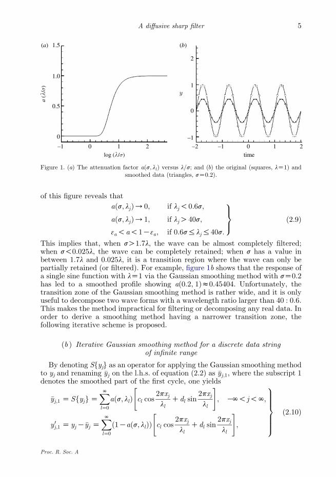
Figure 1. (a) The attenuation factor aðs; llÞ versus l/s; and (b) the original (squares, lZ1) andsmoothed data (triangles, sZ0.2).

5A diffusive sharp filter

of this figure reveals that

aðs; ljÞ/0; if lj!0:6s;

aðs; ljÞ/1; if ljO40s;

3a!a!1K3a; if 0:6s%lj%40s:

9>=>; ð2:9Þ

This implies that, when sO1.7l, the wave can be almost completely filtered;when s!0.025l, the wave can be completely retained; when s has a value inbetween 1.7l and 0.025l, it is a transition region where the wave can only bepartially retained (or filtered). For example, figure 1b shows that the response ofa single sine function with lZ1 via the Gaussian smoothing method with sZ0.2has led to a smoothed profile showing a(0.2, 1)z0.45404. Unfortunately, thetransition zone of the Gaussian smoothing method is rather wide, and it is onlyuseful to decompose two wave forms with a wavelength ratio larger than 40 : 0.6.This makes the method impractical for filtering or decomposing any real data. Inorder to derive a smoothing method having a narrower transition zone, thefollowing iterative scheme is proposed.

(b ) Iterative Gaussian smoothing method for a discrete data stringof infinite range

By denoting S{yj} as an operator for applying the Gaussian smoothing methodto yj and renaming �yj on the l.h.s. of equation (2.2) as �yj;1, where the subscript 1denotes the smoothed part of the first cycle, one yields

�yj;1 Z SfyjgZXNlZ0

aðs; llÞ cl cos2pxjll

Cdl sin2pxjll

" #; KN! j!N;

y 0j;1 Z yjK�yj ZXNlZ0

ð1Kaðs; llÞÞ cl cos2pxjll

Cdl sin2pxjll

" #;

9>>>>>=>>>>>;

ð2:10Þ

Proc. R. Soc. A

Y.-N. Jeng et al.6

where y 0j;1 is the remaining high-frequency part of the first cycle. Likewise, the

remaininghigh-frequency part is smoothed again to obtain yet again the smooth andhigh-frequency parts of the second cycle, say �yj;2 and y 0

j;2, respectively. Repeatingthe procedure up tomth cycle, the corresponding smooth and high-frequency partsare, respectively,

�yj;mZSfy 0j;mK1gZ

XNlZ0

aðs;llÞð1Kaðs;llÞÞmK1 cl cos2pxjll

Cdl sin2pxjll

" #;

y0j;mZXNlZ0

ð1Kaðs;llÞÞm cl cos2pxjll

Cdl sin2pxjll

" #;

9>>>>>=>>>>>;

ð2:11Þ

The accumulated smooth parts, �yjðmÞZ�yj;1C/C�yj;m, are related to the final high-

frequency part through the following relation:

�yjðmÞZðyjKy 0j;1ÞCðy 0

j;1Ky 0j;2ÞCðy 0

j;2Ky 0j;3ÞC/Cðy 0

j;mK1Ky 0j;mÞZyjKy 0

j;m:

ð2:12ÞFor convenience, we rewrite the high-frequency part of equation (2.11) as

y 0j;mZ

XNlZ0

bðs;ll ;mÞ cl cos2pxjll

Cdl sin2pxjll

� �; ð2:13Þ

where

bðs;ll ;mÞZð1Kaðs;llÞÞm: ð2:14Þ

It can be shown that

0%bðs;ll ;mÞ%1Gm3; csO0: ð2:15Þ

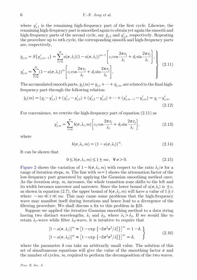
Figure 2 shows the variation of 1Kbðs;ll ;mÞ with respect to the ratio ll=s for arange of iteration steps, m. The line with mZ1 shows the attenuation factor of thelow-frequency part generated by applying the Gaussian smoothing method once.As the iteration step, m, increases, the whole transition zone shifts to the left andits width becomes narrower and narrower. Since the lower bound of aðs;llÞ is G3,as shown in equation (2.7), the upper bound of bðs;ll ;mÞ will have a value of 1G�3where Km3/�3/m3. This may cause some problems that the high-frequencywave may manifest itself during iterations and hence lead to a divergence of thefiltering procedure. We shall discuss a fix to this problem in §2b.

Suppose we applied the iterative Gaussian smoothing method to a data stringhaving two distinct wavelengths, l1 and l2, where l1Ol2. If we would like toretain l1-wave while filter l2-wave, it is intuitive to require that

½1Kaðs; l1Þ�mz 1Kexp K2p2s2=l21� �� m

Z 1Kd;

½1Kaðs; l2Þ�mz 1Kexp K2p2s2=l22� �� m

Z d;

)ð2:16Þ

where the parameter d can take an arbitrarily small value. The solution of thisset of simultaneous equations will give the value of the smoothing factor s andthe number of cycles, m, required to perform the decomposition of the two waves.

Proc. R. Soc. A

2.0(a)

1.5

1.0

0.5

01 2 3 4 5

8(b)

6

log

m

4

2

01 2 3 4 5

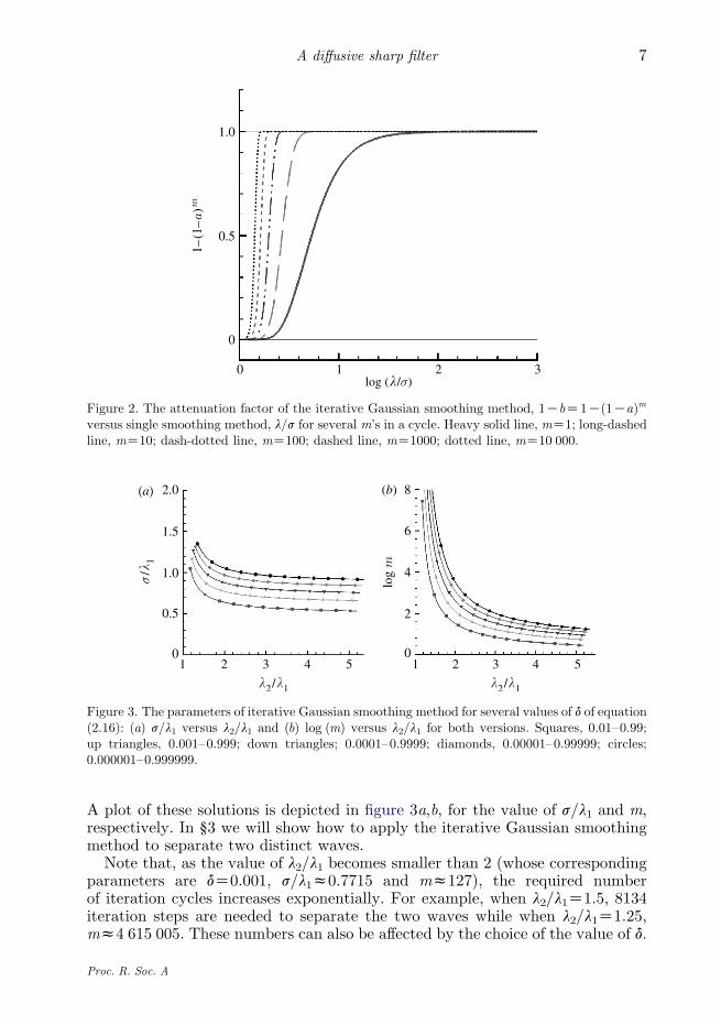
Figure 3. The parameters of iterative Gaussian smoothing method for several values of d of equation(2.16): (a) s/l1 versus l2/l1 and (b) log (m) versus l2/l1 for both versions. Squares, 0.01–0.99;up triangles, 0.001–0.999; down triangles; 0.0001–0.9999; diamonds, 0.00001–0.99999; circles;0.000001–0.999999.

1.0

0.5

0

0 1 2 3

Figure 2. The attenuation factor of the iterative Gaussian smoothing method, 1KbZ1Kð1KaÞmversus single smoothing method, l/s for several m’s in a cycle. Heavy solid line, mZ1; long-dashedline, mZ10; dash-dotted line, mZ100; dashed line, mZ1000; dotted line, mZ10 000.

7A diffusive sharp filter

A plot of these solutions is depicted in figure 3a,b, for the value of s/l1 and m,respectively. In §3 we will show how to apply the iterative Gaussian smoothingmethod to separate two distinct waves.

Note that, as the value of l2/l1 becomes smaller than 2 (whose correspondingparameters are dZ0.001, s/l1z0.7715 and mz127), the required numberof iteration cycles increases exponentially. For example, when l2/l1Z1.5, 8134iteration steps are needed to separate the two waves while when l2/l1Z1.25,mz4 615 005. These numbers can also be affected by the choice of the value of d.

Proc. R. Soc. A

Table 1. Solutions of the required parameters of equation (2.16) for l2/l1Z2.

dZ0.01 dZ0.001 dZ0.0001 dZ0.00001 dZ0.000001

ms 33 127 410 1199 3306ss/l1

a 0.639642 0.771546 0.878266 0.970770 1.053768md 33 127 410 1199 3306sd/l1

a 0.452295 0.545565 0.621028 0.686438 0.745127

aThe superscript of ( )s denotes the iterative Gaussian smoothing method, while ( )d denotes thestrict diffusive iterative Gaussian smoothing method.

Y.-N. Jeng et al.8

As it can be seen from table 1, if the accuracy increases by an order of magnitude,the required value of s/l1 increases slightly while the iteration steps m increaseapproximately three to four orders of magnitude.

It is interesting to see that the underlying principle of the proposed iterationmethod is not very different from the classical iteration methods. For example,the filtering is operated on the smooth part in the current method while in theRay & Ray iterative Gaussian scheme (Ray & Ray 1995) and the Gaussianpyramid (Burt & Adelson 1983; Sonka et al. 1999; Gonzalez & Woods 2002;Misiti et al. 2007), it is the high-frequency part that is repeatedly smoothed.Owing to the fact that the result of applying the Gaussian smoothing method canbe looked upon as the exact solution of the one-dimensional time-dependent heatconduction problem, the result of one smoothing step can be interpreted as thecorresponding solution of the one-dimensional time-dependent heat conductionproblem at the same time instant. The method is therefore akin to a time-marching scheme for solving a partial differential equation by repeatedlyreducing the residue to zero in a sequential manner.

(c ) An iterative Gaussian smoothing method with a strict diffusive property

As shown in equation (2.15), the upper bound of bðs; ll ;mÞ has a value of1Gm3 which may cause some problems. In order to make the iterative proceduresatisfy a strict diffusive property such that 0%bðs; ll ;mÞ%1, the Gaussiansmoothing method is employed to smooth �yj of equation (2.2) once more anddenotes the resulting smoothed part as �yj;1,

�yj;1 ZS2fyjgZXNlZ0

a2ðs; llÞ cl cos2pxjll

Cdl sin2pxjll

" #; KN! j!N;

y 0j;1 Z yjK�yj;1 Z

XNlZ0

ð1Ka2ðs; llÞÞ cl cos2pxjll

Cdl sin2pxjll

" #;

9>>>>>=>>>>>;

ð2:17Þ

where S 2{yj} denotes the application of the Gaussian smoothing method, firstlyto yj and then to �yj once again. The mth cycle’s results are

�yj;m ZS 2 y 0j;mK1

� �Z

XNlZ0

a2ðs; llÞð1Ka2ðs; llÞÞmK1 cl cos2pxjll

Cdl sin2pxjll

� �;

Proc. R. Soc. A

9A diffusive sharp filter

y 0j;m Z

XNlZ0

ð1Ka2ðs; llÞÞm cl cos2pxjll

Cdl sin2pxjll

" #

ZXNlZ0

bðs; ll ;mÞ cl cos2pxjll

Cdl sin2pxjll

" #; KN! j!N; mZ 1; 2;. :

ð2:18Þ

Owing to the strict non-negative property of a2, the factor bðs; ll ;mÞ satisfies

0%bðs; ll ;mÞZ 1Ka2ðs; llÞ� m

%1: ð2:19Þ

In other words, this iterative procedure is a strict diffusive smoothing method,and the corresponding variation of this new attenuation factor, 1Kbðs; ll ;mÞ,with respect to l/s is exactly the same as the one shown in figure 2, providedthat s is replaced by s=

ffiffiffi2

p.

The estimated smoothing factor sd and iteration md (the subscript ‘d’ standsfor the double smoothing that leads to the strict diffusive method) are solvedfrom equation (2.16) with the factor a(s, ll) replaced by a2(s, ll) and the factor 2of the exponential function replaced by 4, respectively. The correspondingparameters sd=

ffiffiffi2

pand md for different values of d are exactly the same as shown

in figure 3a,b, respectively. It is noted that the required computing time ofemploying the strict diffusive iterative Gaussian smoothing method is twice thatfor the iterative Gaussian smoothing method.

(d ) Filtering a discrete data string with finite length

In practice, data are not periodic and therefore they cannot be interpreted asinfinite data strings. The extension of the two proposed iterative Gaussiansmoothing methods to a data string of finite length is discussed in this section.

For a finite-range data string, say (xj, yj), jZ0, 1, 2,., n, the correspondingdiscrete Fourier expansion is

yj ZXnK1

lZ0

cl cos2pxjll

Cdl sin2pxjll

� �; j Z 0; 1; 2;.;nK1: ð2:20Þ

The application of the Gaussian smoothing method, which is the zeroth-ordermoving least-squares method for a finite data length, will give

�yj Z1�kj

XnK1

iZ0

exp ðKðxiKxjÞ2=ð2s2ÞÞXnK1

lZ0

cl cos2pxill

Cdl sin2pxill

" #;

�kj ZXnK1

iZ0

exp ðKðxiKxjÞ2=ð2s2ÞÞ:

9>>>>>=>>>>>;

ð2:21Þ

Unlike k of equation (2.2), �kj is not a constant but changes with respect to xj now.Following the similar transform to obtain equation (2.4), the following relations

Proc. R. Soc. A

Y.-N. Jeng et al.10

are obtained:

�yj Z1�kj

XnK1

lZ0

cl cos2pxjll

Cdl sin2pxjll

� �XnK1

iZ0

exp ðKðxiK xjÞ2=ð2s2ÞÞ cos2pðxiK xjÞ

ll

(

C dl cos2pxjll

K cl sin2pxjll

� �XnK1

iZ0

exp ðKðxiK xjÞ2=ð2s2ÞÞ sin2pðxiK xjÞ

ll

)

Z1�kj

XnK1

lZ0

cl cos2pxjll

Cdl sin2pxjll

� � XnK1Kj

iZKj

exp ðKx2i =ð2s2ÞÞ cos2pxill

(

C dl cos2pxjll

K cl sin2pxjll

� � XnK1Kj

iZKj

exp ðKx2i =ð2s2ÞÞ sin2pxill

): ð2:22Þ

If xmO5s where mZmin ðj;nK1KjÞ, the magnitude of the Gaussian functions,exp ½Kx2m=ð2s2Þ�, is of the order of O(K6) and is of no significance and henceequation (2.22) can be considered to be unaffected by the finite-lengthassumption of the data

1�kj

XnK1Kj

iZKj

exp ðKx2i =ð2s2ÞÞ cos2pxill

z1

k

XNiZKN

exp ðKx 2i =ð2s2ÞÞ cos

2pxill

Z aðs; llÞ;

XnK1Kj

iZKj

exp ðKx2i =ð2s2ÞÞ sin2pxill

zXNiZKN

exp ðKx2i =ð2s2ÞÞ sin2pxill

Z 0: ð2:23Þ

As a result, equation (2.22) can be written as

�yjzXNlZ0

aðs; llÞ cl cos2pxjll

Cdl sin2pxjll

� �: ð2:24Þ

On the other hand when data points are close to the boundary, the upper boundof the difference between smoothing for finite data points and infinite data points,�yj and �yN

j , respectively, can be estimated as

�yjK�yNj

Z 1�kj

XniZ0

exp KðiKjÞ2ðDxÞ2

2s2

� �yiK

1

j

XNiZKN

exp KðiKjÞ2ðDxÞ2

2s2

� �yi

%ymax

�kjFðKjDxÞC 1

�kjK

1

k

k�yNj z 2FðKjDxÞ

1KFðKjDxÞ ymax;1; ð2:25Þ

where F is the error function and ymax;1Zmaxjz0½�ymax; �yNj � in which �ymaxZmaxiz0

½�yi!0� and the index, iz0, implies the points in the vicinity of region whereexp ½KðiKjÞ2ðDxÞ2=2s2�z1.

Proc. R. Soc. A

51st cycle2nd cycle5th cycle10th cycle50th cycle100th cycle127th cycle

0

–5

–100 10 20 30

iteration cycles

log

(err

or)

40

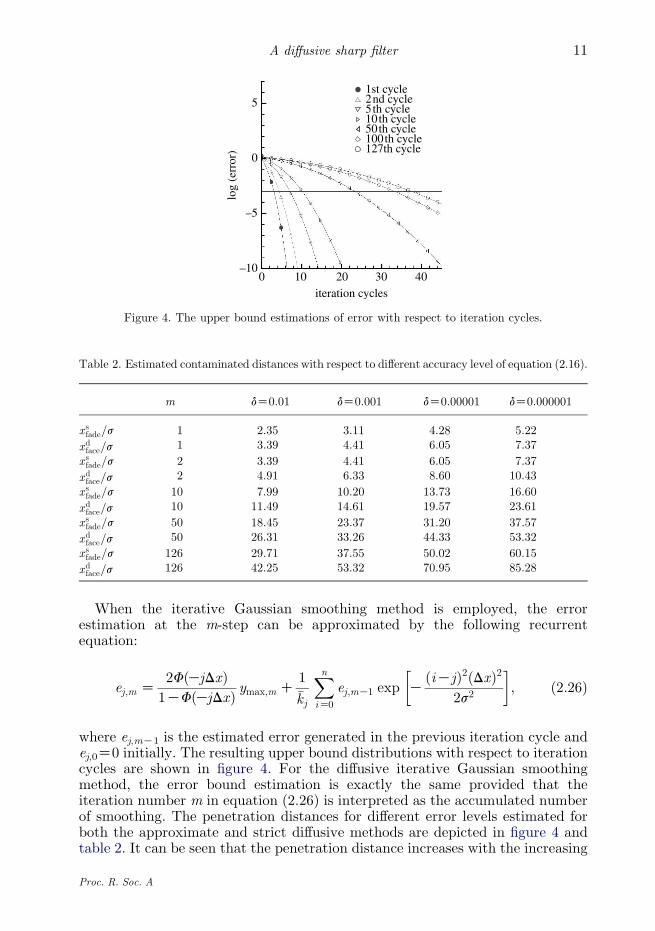
Figure 4. The upper bound estimations of error with respect to iteration cycles.

Table 2. Estimated contaminated distances with respect to different accuracy level of equation (2.16).

m dZ0.01 dZ0.001 dZ0.00001 dZ0.000001

x sfade=s 1 2.35 3.11 4.28 5.22

xdface=s 1 3.39 4.41 6.05 7.37

x sfade=s 2 3.39 4.41 6.05 7.37

xdface=s 2 4.91 6.33 8.60 10.43

x sfade=s 10 7.99 10.20 13.73 16.60

xdface=s 10 11.49 14.61 19.57 23.61

x sfade=s 50 18.45 23.37 31.20 37.57

xdface=s 50 26.31 33.26 44.33 53.32

x sfade=s 126 29.71 37.55 50.02 60.15

xdface=s 126 42.25 53.32 70.95 85.28

11A diffusive sharp filter

When the iterative Gaussian smoothing method is employed, the errorestimation at the m-step can be approximated by the following recurrentequation:

ej;m Z2FðKjDxÞ

1KFðKjDxÞ ymax;m C1�kj

XniZ0

ej;mK1 exp KðiKjÞ2ðDxÞ2

2s2

� �; ð2:26Þ

where ej,mK1 is the estimated error generated in the previous iteration cycle andej,0Z0 initially. The resulting upper bound distributions with respect to iterationcycles are shown in figure 4. For the diffusive iterative Gaussian smoothingmethod, the error bound estimation is exactly the same provided that theiteration number m in equation (2.26) is interpreted as the accumulated numberof smoothing. The penetration distances for different error levels estimated forboth the approximate and strict diffusive methods are depicted in figure 4 andtable 2. It can be seen that the penetration distance increases with the increasing

Proc. R. Soc. A

Y.-N. Jeng et al.12

number of iterations in an approximately exponential manner. It is noted thatfigure 4 and table 2 give the maximum possible errors and therefore theestimated distance of influence can be much larger than real numerical tests.This exercise only serves to give an indication of how the error propagateswith iterations.

(e ) The algorithm for the iterative smoothing procedure

The algorithm for the proposed iterative procedure can be summarized asfollows.

(i) Select the scheme of the iterative Gaussian smoothing method—be it adiffusive or a strict diffusive procedure.

(ii) Determine the transition zone, say l1 and l2. It is recommended to allowthe transition zone to satisfy l2/l1R2 as discussed in §2b.

(iii) Determine values of s and m by solving equation (2.16). If the strictdiffusive version is employed, the resulting s is replaced by s=

ffiffiffi2

p.

(iv) Repeatedly apply the corresponding iterative method with the parameters for m iteration cycles.

(v) The resulting high-frequency part is the desired high-frequency part andthe difference between the original data and the high-frequency partbecomes the smooth part.

3. Results and discussions

In order to examine the proposed iteration procedure, the following compositewaveform is made up of two independent waves having wavelengths 0.5 and 0.25,respectively:

yðxÞZ sin ð4pxÞCsin ð8pxÞ: ð3:1Þ

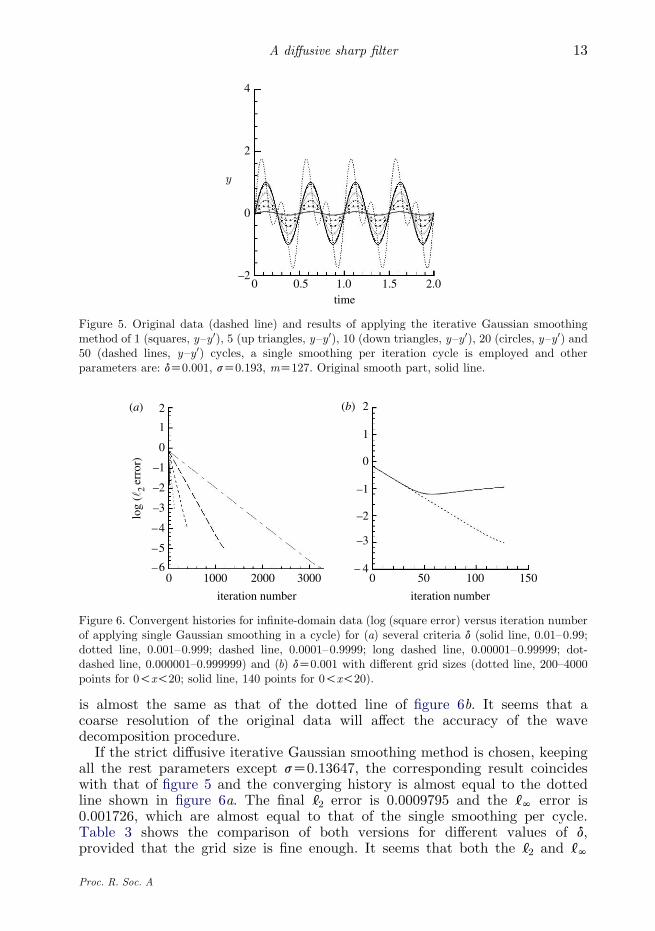
If dZ0.001 and the iterative Gaussian smoothing method are chosen, table 1suggests that the critical s and m are 0.193 and 127, respectively. In order tosimulate the infinite-domain limit, the calculation is taken in the range of 0%xj%10andK10%xi%20 with DxZ0.005 where xi and xj are defined in equations (2.1) and(2.2), respectively. After all the data at xj’s are evaluated in every cycle, they areperiodically mapped to those points xi in the range ofK10!xi!0 and 10!xi!20,respectively. These conditions ensure that exp ½KðxiK xjÞ2=ð2s2Þ�!10K50 for alljxiKxjjO10 and 0%xj%10 simultaneously. Figure 5 shows the resulting accumu-lated smooth part of the 1st, 5th, 10th, 20th and 50th iteration cycles. It isclear that the smooth part gradually approaches the original long-wave mode.The converging history is shown as the dotted line in figure 6a, whichshows an exponential decay of the [2 error and confirms the estimation of theattenuation factor a(s, ll) in equation (2.6). The final [2 error is 0.0009794 whilethe [N error of 0.001726 shows that the maximum error will be slightly largerthan dZ0.001. Figure 6a also shows the convergent histories for several differentd values, all of which show similar exponential convergent behaviour. In figure 6b,there is a solid line that shows a non-convergent behaviour with DxZ1/7and all the other parameters are the same as that of the dotted line (fine-gridsolution). Numerical experiments show that if Dx!1/8, the convergent history

Proc. R. Soc. A

4

2

y

0

–20 0.5 1.0

time1.5 2.0

Figure 5. Original data (dashed line) and results of applying the iterative Gaussian smoothingmethod of 1 (squares, y–y 0), 5 (up triangles, y–y 0), 10 (down triangles, y–y0), 20 (circles, y–y0) and50 (dashed lines, y–y0) cycles, a single smoothing per iteration cycle is employed and otherparameters are: dZ0.001, sZ0.193, mZ127. Original smooth part, solid line.

2

1

0

–1

–2

–3

–4

–5

–60 1000 2000

iteration number iteration number

log

(�2

erro

r)

3000

(a) 2

1

0

–1

–2

–3

– 40 50 100 150

(b)

Figure 6. Convergent histories for infinite-domain data (log (square error) versus iteration numberof applying single Gaussian smoothing in a cycle) for (a) several criteria d (solid line, 0.01–0.99;dotted line, 0.001–0.999; dashed line, 0.0001–0.9999; long dashed line, 0.00001–0.99999; dot-dashed line, 0.000001–0.999999) and (b) dZ0.001 with different grid sizes (dotted line, 200–4000points for 0!x!20; solid line, 140 points for 0!x!20).

13A diffusive sharp filter

is almost the same as that of the dotted line of figure 6b. It seems that acoarse resolution of the original data will affect the accuracy of the wavedecomposition procedure.

If the strict diffusive iterative Gaussian smoothing method is chosen, keepingall the rest parameters except sZ0.13647, the corresponding result coincideswith that of figure 5 and the converging history is almost equal to the dottedline shown in figure 6a. The final [2 error is 0.0009795 and the [N error is0.001726, which are almost equal to that of the single smoothing per cycle.Table 3 shows the comparison of both versions for different values of d,provided that the grid size is fine enough. It seems that both the [2 and [N

Proc. R. Soc. A

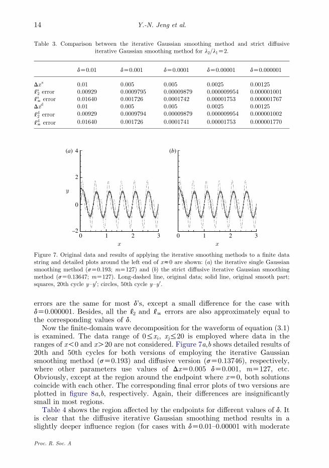
Table 3. Comparison between the iterative Gaussian smoothing method and strict diffusiveiterative Gaussian smoothing method for l2/l1Z2.

dZ0.01 dZ0.001 dZ0.0001 dZ0.00001 dZ0.000001

Dx s 0.01 0.005 0.005 0.0025 0.00125[ s2 error 0.00929 0.0009795 0.00009879 0.000009954 0.000001001[ sN error 0.01640 0.001726 0.0001742 0.00001753 0.000001767Dxd 0.01 0.005 0.005 0.0025 0.00125

[ d2 error 0.00929 0.0009794 0.00009879 0.000009954 0.000001002

[ dN error 0.01640 0.001726 0.0001741 0.00001753 0.000001770

4

2

0

–2

y

(a) (b)

0 1 2 30 1 2 3

Figure 7. Original data and results of applying the iterative smoothing methods to a finite datastring and detailed plots around the left end of xz0 are shown: (a) the iterative single Gaussiansmoothing method (sZ0.193; mZ127) and (b) the strict diffusive iterative Gaussian smoothingmethod (sZ0.13647; mZ127). Long-dashed line, original data; solid line, original smooth part;squares, 20th cycle y–y0; circles, 50th cycle y–y 0.

Y.-N. Jeng et al.14

errors are the same for most d’s, except a small difference for the case withdZ0.000001. Besides, all the [2 and [N errors are also approximately equal tothe corresponding values of d.

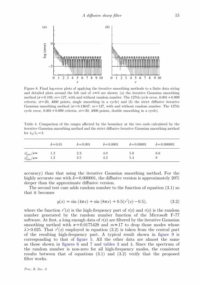
Now the finite-domain wave decomposition for the waveform of equation (3.1)is examined. The data range of 0%xi , xj%20 is employed where data in theranges of x!0 and xO20 are not considered. Figure 7a,b shows detailed results of20th and 50th cycles for both versions of employing the iterative Gaussiansmoothing method (sZ0.193) and diffusive version (sZ0.13746), respectively,where other parameters use values of DxZ0.005 dZ0.001, mZ127, etc.Obviously, except at the region around the endpoint where xZ0, both solutionscoincide with each other. The corresponding final error plots of two versions areplotted in figure 8a,b, respectively. Again, their differences are insignificantlysmall in most regions.

Table 4 shows the region affected by the endpoints for different values of d. Itis clear that the diffusive iterative Gaussian smoothing method results in aslightly deeper influence region (for cases with dZ0.01–0.00001 with moderate

Proc. R. Soc. A

0

(a) (b)

0 1 2 3 4 5 6 7 8 9 100 1 2 3 4 5 6 7 8 9 10

–5

log

(err

or)

Figure 8. Final log-error plots of applying the iterative smoothing methods to a finite data stringand detailed plots around the left end of xz0 are shown: (a) the iterative Gaussian smoothingmethod (sZ0.193; mZ127, with and without random number. The 127th cycle error, 0.001C0.999criteria; xtZ20, 4000 points, single smoothing in a cycle) and (b) the strict diffusive iterativeGaussian smoothing method (sZ0.13647; mZ127, with and without random number. The 127thcycle error, 0.001C0.999 criteria; xtZ20, 4000 points, double smoothing in a cycle).

Table 4. Comparison of the ranges affected by the boundary at the two ends calculated by theiterative Gaussian smoothing method and the strict diffusive iterative Gaussian smoothing methodfor l2/l1Z2.

dZ0.01 dZ0.001 dZ0.0001 dZ0.00001 dZ0.000001

x sfade=sz 1.2 2.3 4.0 5.0 6.6

xdfade=sz 1.2 2.5 4.2 5.4 8

15A diffusive sharp filter

accuracy) than that using the iterative Gaussian smoothing method. For thehighly accurate one with dZ0.000001, the diffusive version is approximately 20%deeper than the approximate diffusive version.

The second test case adds random number to the function of equation (3.1) sothat it becomes

yðxÞZ sin ð4pxÞCsin ð8pxÞC0:5ðr 0ðxÞK0:5Þ; ð3:2Þ

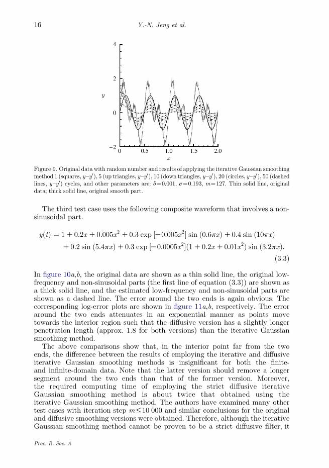
where the function r0(x) is the high-frequency part of r(x) and r(x) is the randomnumber generated by the random number function of the Microsoft F-77software. At first, a long enough data of r(x) are filtered by the iterative Gaussiansmoothing method with sZ0.0175428 and mz17 to drop those modes whoselO0.025. That r0(x) employed in equation (3.2) is taken from the central partof the resulting high-frequency part. A typical result shown in figure 9 iscorresponding to that of figure 5. All the other data are almost the sameas those shown in figures 6 and 7 and tables 3 and 4. Since the spectrum ofthe random number is non-zero for all high-frequency modes, the consistentresults between that of equations (3.1) and (3.2) verify that the proposedfilter works.

Proc. R. Soc. A

4

2

0

0 0.5 1.0 1.5 2.0–2

Figure 9. Original data with random number and results of applying the iterative Gaussian smoothingmethod 1 (squares, y–y0), 5 (up triangles, y–y0), 10 (down triangles, y–y0), 20 (circles, y–y0), 50 (dashedlines, y–y0) cycles, and other parameters are: dZ0.001, sZ0.193, mZ127. Thin solid line, originaldata; thick solid line, original smooth part.

Y.-N. Jeng et al.16

The third test case uses the following composite waveform that involves a non-sinusoidal part.

yðtÞZ 1C0:2xC0:005x2 C0:3 exp ½K0:005x2� sin ð0:6pxÞC0:4 sin ð10pxÞC0:2 sin ð5:4pxÞC0:3 exp ½K0:0005x2�ð1C0:2xC0:01x2Þ sin ð3:2pxÞ:

ð3:3Þ

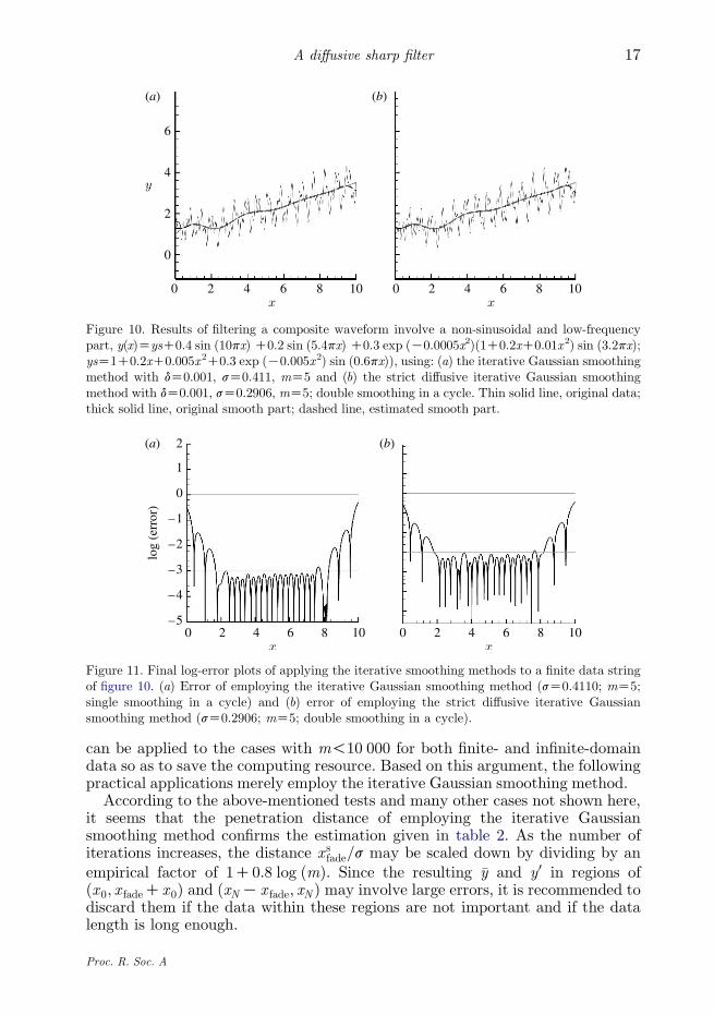
In figure 10a,b, the original data are shown as a thin solid line, the original low-frequency and non-sinusoidal parts (the first line of equation (3.3)) are shown asa thick solid line, and the estimated low-frequency and non-sinusoidal parts areshown as a dashed line. The error around the two ends is again obvious. Thecorresponding log-error plots are shown in figure 11a,b, respectively. The erroraround the two ends attenuates in an exponential manner as points movetowards the interior region such that the diffusive version has a slightly longerpenetration length (approx. 1.8 for both versions) than the iterative Gaussiansmoothing method.

The above comparisons show that, in the interior point far from the twoends, the difference between the results of employing the iterative and diffusiveiterative Gaussian smoothing methods is insignificant for both the finite-and infinite-domain data. Note that the latter version should remove a longersegment around the two ends than that of the former version. Moreover,the required computing time of employing the strict diffusive iterativeGaussian smoothing method is about twice that obtained using theiterative Gaussian smoothing method. The authors have examined many othertest cases with iteration step m%10 000 and similar conclusions for the originaland diffusive smoothing versions were obtained. Therefore, although the iterativeGaussian smoothing method cannot be proven to be a strict diffusive filter, it

Proc. R. Soc. A

6

(a)

4

2

y

0

(b)

0 2 4x

6 8 100 2 4x

6 8 10

Figure 10. Results of filtering a composite waveform involve a non-sinusoidal and low-frequencypart, y(x)ZysC0.4 sin (10px) C0.2 sin (5.4px) C0.3 exp (K0.0005x2)(1C0.2xC0.01x2) sin (3.2px);ysZ1C0.2xC0.005x2C0.3 exp (K0.005x2) sin (0.6px)), using: (a) the iterative Gaussian smoothingmethod with dZ0.001, sZ0.411, mZ5 and (b) the strict diffusive iterative Gaussian smoothingmethod with dZ0.001, sZ0.2906, mZ5; double smoothing in a cycle. Thin solid line, original data;thick solid line, original smooth part; dashed line, estimated smooth part.

2(a) (b)

1

0

–1

–2

–3

–4

–5

log

(err

or)

0 2 4 6 8 100 2 4 6 8 10

Figure 11. Final log-error plots of applying the iterative smoothing methods to a finite data stringof figure 10. (a) Error of employing the iterative Gaussian smoothing method (sZ0.4110; mZ5;single smoothing in a cycle) and (b) error of employing the strict diffusive iterative Gaussiansmoothing method (sZ0.2906; mZ5; double smoothing in a cycle).

17A diffusive sharp filter

can be applied to the cases with m!10 000 for both finite- and infinite-domaindata so as to save the computing resource. Based on this argument, the followingpractical applications merely employ the iterative Gaussian smoothing method.

According to the above-mentioned tests and many other cases not shown here,it seems that the penetration distance of employing the iterative Gaussiansmoothing method confirms the estimation given in table 2. As the number ofiterations increases, the distance x sfade=s may be scaled down by dividing by anempirical factor of 1C0:8 log ðmÞ. Since the resulting �y and y0 in regions ofðx0; x fadeCx0Þ and ðxNK x fade; xN Þ may involve large errors, it is recommended todiscard them if the data within these regions are not important and if the datalength is long enough.

Proc. R. Soc. A

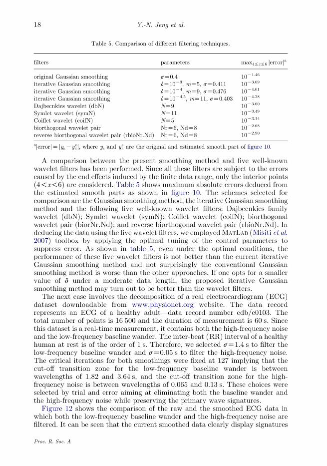
Table 5. Comparison of different filtering techniques.

filters parameters max4%x%6 jerrorja

original Gaussian smoothing sZ0.4 10K1.46

iterative Gaussian smoothing dZ10K3, mZ5, sZ0.411 10K3.09

iterative Gaussian smoothing dZ10K4, mZ9, sZ0.476 10K4.01

iterative Gaussian smoothing dZ10K4.5, mZ11, sZ0.403 10K4.28

Dajbecnkies wavelet (dbN) NZ9 10K3.00

Symlet wavelet (symN) NZ11 10K3.49

Coiflet wavelet (coifN) NZ5 10K3.14

biorthogonal wavelet pair NrZ6, NdZ8 10K2.68

reverse biorthogonal wavelet pair (rbioNr.Nd) NrZ6, NdZ8 10K2.90

ajerrorjZ jysKyes j, where ys and ye

s are the original and estimated smooth part of figure 10.

Y.-N. Jeng et al.18

A comparison between the present smoothing method and five well-knownwavelet filters has been performed. Since all these filters are subject to the errorscaused by the end effects induced by the finite data range, only the interior points(4!x!6) are considered. Table 5 shows maximum absolute errors deduced fromthe estimated smooth parts as shown in figure 10. The schemes selected forcomparison are the Gaussian smoothingmethod, the iterative Gaussian smoothingmethod and the following five well-known wavelet filters: Dajbecnkies familywavelet (dbN); Symlet wavelet (symN); Coiflet wavelet (coifN); biorthogonalwavelet pair (biorNr.Nd); and reverse biorthogonal wavelet pair (rbioNr.Nd). Indeducing the data using the five wavelet filters, we employedMATLAB (Misiti et al.2007) toolbox by applying the optimal tuning of the control parameters tosuppress error. As shown in table 5, even under the optimal conditions, theperformance of these five wavelet filters is not better than the current iterativeGaussian smoothing method and not surprisingly the conventional Gaussiansmoothing method is worse than the other approaches. If one opts for a smallervalue of d under a moderate data length, the proposed iterative Gaussiansmoothing method may turn out to be better than the wavelet filters.

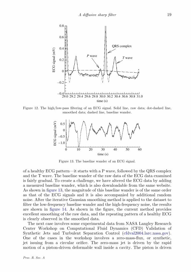
The next case involves the decomposition of a real electrocardiogram (ECG)dataset downloadable from www.physionet.org website. The data recordrepresents an ECG of a healthy adult—data record number edb/e0103. Thetotal number of points is 16 500 and the duration of measurement is 60 s. Sincethis dataset is a real-time measurement, it contains both the high-frequency noiseand the low-frequency baseline wander. The inter-beat (RR) interval of a healthyhuman at rest is of the order of 1 s. Therefore, we selected sZ1.4 s to filter thelow-frequency baseline wander and sZ0.05 s to filter the high-frequency noise.The critical iterations for both smoothings were fixed at 127 implying that thecut-off transition zone for the low-frequency baseline wander is betweenwavelengths of 1.82 and 3.64 s, and the cut-off transition zone for the high-frequency noise is between wavelengths of 0.065 and 0.13 s. These choices wereselected by trial and error aiming at eliminating both the baseline wander andthe high-frequency noise while preserving the primary wave signatures.

Figure 12 shows the comparison of the raw and the smoothed ECG data inwhich both the low-frequency baseline wander and the high-frequency noise arefiltered. It can be seen that the current smoothed data clearly display signatures

Proc. R. Soc. A

0.8

0.6

0.4

0.2

EC

G s

igna

l (m

V)

0

–0.2

–0.4

QRS complex

T waveP wave

29.0 29.2 29.4 29.6 29.8 30.0time (s)

30.2 30.4 30.6 30.8 31.0

Figure 12. The high/low-pass filtering of an ECG signal. Solid line, raw data; dot-dashed line,smoothed data; dashed line, baseline wander.

0.5

0

0 10 20 30time (s)

40 50 60

–0.5

–1.0EC

G s

igna

l (m

V)

Figure 13. The baseline wander of an ECG signal.

19A diffusive sharp filter

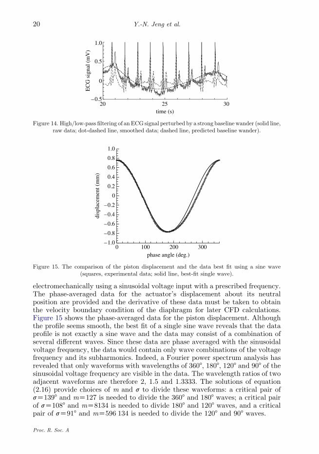
of a healthy ECG pattern—it starts with a P wave, followed by the QRS complexand the T wave. The baseline wander of the raw data of the ECG data examinedis fairly gradual. To create a challenge, we have altered the ECG data by addinga measured baseline wander, which is also downloadable from the same website.As shown in figure 13, the magnitude of this baseline wander is of the same orderas that of the ECG signals and it is also accompanied by additional randomnoise. After the iterative Gaussian smoothing method is applied to the dataset tofilter the low-frequency baseline wander and the high-frequency noise, the resultsare shown in figure 14. As shown in the figure, the current method providesexcellent smoothing of the raw data, and the repeating pattern of a healthy ECGis clearly observed in the smoothed data.

The next case involves some experimental data from NASA Langley ResearchCenter Workshop on Computational Fluid Dynamics (CFD) Validation ofSynthetic Jets and Turbulent Separation Control (cfdval2004.larc.nasa.gov).One of the cases in the workshop involves a zero-mass-flux, or synthetic,jet issuing from a circular orifice. The zero-mass jet is driven by the rapidmotion of a piston-driven deformable wall inside a cavity. The piston is driven

Proc. R. Soc. A

1.0

0.8

0.6

0.4

0.2

0

–0.2

–0.4

–0.6

–0.8

–1.00 100 200

phase angle (deg.)

disp

lace

men

t (m

m)

300

Figure 15. The comparison of the piston displacement and the data best fit using a sine wave(squares, experimental data; solid line, best-fit single wave).

1.0

0.5

0E

CG

sig

nal (

mV

)

time (s)

–0.520 25 30

Figure 14. High/low-pass filtering of an ECG signal perturbed by a strong baseline wander (solid line,raw data; dot-dashed line, smoothed data; dashed line, predicted baseline wander).

Y.-N. Jeng et al.20

electromechanically using a sinusoidal voltage input with a prescribed frequency.The phase-averaged data for the actuator’s displacement about its neutralposition are provided and the derivative of these data must be taken to obtainthe velocity boundary condition of the diaphragm for later CFD calculations.Figure 15 shows the phase-averaged data for the piston displacement. Althoughthe profile seems smooth, the best fit of a single sine wave reveals that the dataprofile is not exactly a sine wave and the data may consist of a combination ofseveral different waves. Since these data are phase averaged with the sinusoidalvoltage frequency, the data would contain only wave combinations of the voltagefrequency and its subharmonics. Indeed, a Fourier power spectrum analysis hasrevealed that only waveforms with wavelengths of 3608, 1808, 1208 and 908 of thesinusoidal voltage frequency are visible in the data. The wavelength ratios of twoadjacent waveforms are therefore 2, 1.5 and 1.3333. The solutions of equation(2.16) provide choices of m and s to divide these waveforms: a critical pair ofsZ1398 and mZ127 is needed to divide the 3608 and 1808 waves; a critical pairof sZ1088 and mZ8134 is needed to divide 1808 and 1208 waves, and a criticalpair of sZ918 and mZ596 134 is needed to divide the 1208 and 908 waves.

Proc. R. Soc. A

1.0

0.8

0.6

0.4

0.2

0

–0.2

–0.4

–0.6

–0.8

–1.00 100 200

phase angle (deg.)

disp

lace

men

t (m

m)

300

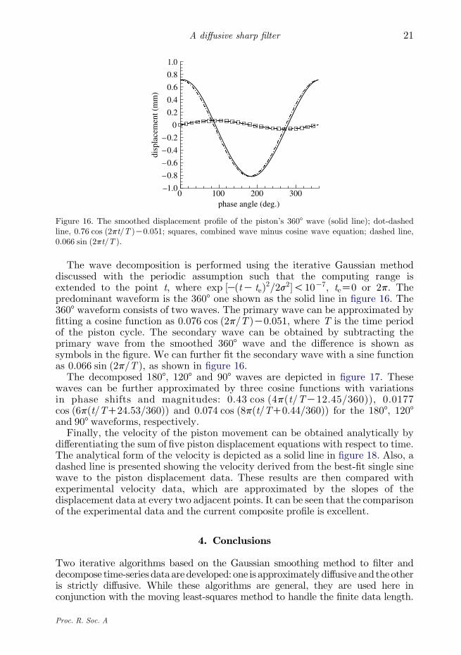
Figure 16. The smoothed displacement profile of the piston’s 3608 wave (solid line); dot-dashedline, 0.76 cos (2pt/T )K0.051; squares, combined wave minus cosine wave equation; dashed line,0.066 sin (2pt/T ).

21A diffusive sharp filter

The wave decomposition is performed using the iterative Gaussian methoddiscussed with the periodic assumption such that the computing range isextended to the point t, where exp ½KðtK teÞ2=2s2�!10K7, teZ0 or 2p. Thepredominant waveform is the 3608 one shown as the solid line in figure 16. The3608 waveform consists of two waves. The primary wave can be approximated byfitting a cosine function as 0.076 cos (2p/T )K0.051, where T is the time periodof the piston cycle. The secondary wave can be obtained by subtracting theprimary wave from the smoothed 3608 wave and the difference is shown assymbols in the figure. We can further fit the secondary wave with a sine functionas 0.066 sin (2p/T ), as shown in figure 16.

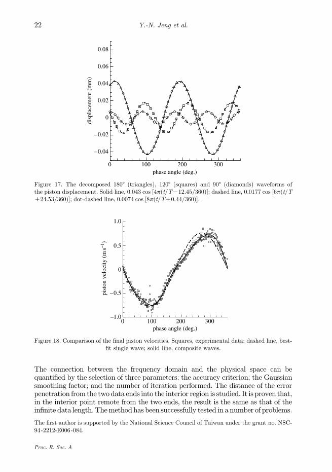
The decomposed 1808, 1208 and 908 waves are depicted in figure 17. Thesewaves can be further approximated by three cosine functions with variationsin phase shifts and magnitudes: 0.43 cos (4p(t/TK12.45/360)), 0.0177cos (6p(t/TC24.53/360)) and 0.074 cos (8p(t/TC0.44/360)) for the 1808, 1208and 908 waveforms, respectively.

Finally, the velocity of the piston movement can be obtained analytically bydifferentiating the sum of five piston displacement equations with respect to time.The analytical form of the velocity is depicted as a solid line in figure 18. Also, adashed line is presented showing the velocity derived from the best-fit single sinewave to the piston displacement data. These results are then compared withexperimental velocity data, which are approximated by the slopes of thedisplacement data at every two adjacent points. It can be seen that the comparisonof the experimental data and the current composite profile is excellent.

4. Conclusions

Two iterative algorithms based on the Gaussian smoothing method to filter anddecompose time-series dataaredeveloped: one is approximatelydiffusive and theotheris strictly diffusive. While these algorithms are general, they are used here inconjunction with the moving least-squares method to handle the finite data length.

Proc. R. Soc. A

1.0

0.5

pist

on v

eloc

ity (

ms–1

)

0

–0.5

–1.00 100 200

phase angle (deg.)300

Figure 18. Comparison of the final piston velocities. Squares, experimental data; dashed line, best-fit single wave; solid line, composite waves.

0.08

0.06

0.04di

spla

cem

ent (

mm

)

0.02

0

–0.02

–0.04

0 100 200phase angle (deg.)

300

Figure 17. The decomposed 1808 (triangles), 1208 (squares) and 908 (diamonds) waveforms ofthe piston displacement. Solid line, 0.043 cos [4p(t/TK12.45/360)]; dashed line, 0.0177 cos [6p(t/TC24.53/360)]; dot-dashed line, 0.0074 cos [8p(t/TC0.44/360)].

Y.-N. Jeng et al.22

The connection between the frequency domain and the physical space can bequantified by the selection of three parameters: the accuracy criterion; the Gaussiansmoothing factor; and the number of iteration performed. The distance of the errorpenetration from the twodata ends into the interior region is studied. It is proven that,in the interior point remote from the two ends, the result is the same as that of theinfinite data length. Themethod has been successfully tested in a number of problems.

The first author is supported by the National Science Council of Taiwan under the grant no. NSC-

94-2212-E006-084.

Proc. R. Soc. A

23A diffusive sharp filter

References

Burt, P. J. & Adelson, E. H. 1983 The Laplacian pyramid as a compact image code. IEEE Trans.Commun. 31, 532–540. (doi:10.1109/TCOM.1983.1095851)

Carslaw, H. S. & Jaeger, J. C. 1957 Conduction of heat in solids. New York, NY: Oxford UniversityPress.

Fasshauer, G. 2002 Approximate moving least-squares approximations: a fast and accuratemultivariate approximation method. Curve Surf. Fitting 1, 1–10.

Gonzalez, R. C. & Woods, R. E. 2002 Digital image processing, 2nd edn. Upper Saddle River, NJ:Pearson Education, Inc.

Goswami, J. C. & Chan, A. K. 1999 Fundamentals of wavelets, theory, algorithms, andapplications. New York, NY: Wiley.

Hess-Nielsen, N. & Wickerhauser, M. V. 1996 Wavelets and time-frequency analysis. Proc. IEEE84, 523–540. (doi:10.1109/5.488698)

Hua, R. & Sarkar, T. K. 1989 Generalized pencil-of-function method for extracting poles of an EMsystem from its transient response. IEEE Trans. Anten. Propag. 37, 229–234. (doi:10.1109/8.18710)

Huang, N. E., Shen, Z., Long, S. R., Wu, M. C., Shih, H. H., Zheng, Q., Yen, N.-C., Tung, C. C. &Liu, H. H. 1998 The empirical mode decomposition and the Hilbert spectrum for nonlinear andnon-stationary time series analysis. Proc. R. Soc. A 454, 903–995. (doi:10.1098/rspa.1998.0193)

Huang, N. E., Shen, Z. & Long, S. R. 1999 A new view of nonlinear water waves: the Hilbertspectrum. Annu. Rev. Fluid Mech. 51, 417–457. (doi:10.1146/annurev.fluid.31.1.417)

Jeng, Y. N. 2000 The moving least-squares and least p -power methods for random data. In Proc.7th National Computational Fluid Dynamics Conference, Kenting, Taiwan, August, pp. 9–14.The Netherlands: Kluwer Academic Publishers.

Jeng, Y. N. & Cheng, Y. C. 2004 A simple strategy to evaluate the frequency spectrum of a timeseries data with non-uniform intervals. Trans. Aeronaut. Astronaut. Soc. (Republic of China)36, 207–214.

Lancaster, P. & Salkauskas, K. 1986 Curve and surface fitting: an introduction, ch. 2, 10.New York, NY, Academic Press.

Liew, K. M., Huang, Y. Q. & Reddy, J. N. 2002 A hybrid moving least-squares and differentialquadrature (MLSDQ) meshfree method. Int. J. Comput. Eng. Sci. 3, 1–12. (doi:10.1142/S1465876302000526)

Lowe, D. G. 1989 Organization of smooth image curves at multiple scales. Int. J. Comput. Vis. 3,119–130. (doi:10.1007/BF00126428)

Mackworth, A. K. & Mokhtarian, F. 1984 Scale-based description of planar curves. In Proc.5thCanadianSociety forComputational Studies of Intelligence, London,Ontario,May, pp. 114–119.

Marr, D. & Hildreth, E. 1980 Theory of edge detection. Proc. R. Soc. B 207, 187–217. (doi:10.1098/rspb.1980.0020)

Misiti, M., Misiti, Y., Oppenheim, G. & Poggi, J. M. 2007 Wavlet toolbox 4 user’s guide. Natick,MA: The MathWorks, Inc.

Mokhtarian, F. & Mackworth, A. 1986 Scale-based description and recognition of planar curvesand two-dimensional shapes. IEEE Trans. Pattern Anal. Mach. Intell. 8, 34–43.

Morse, P. M. & Feshbach, H. 1953Methods of theoretical physics, vol. 2. NewYork, NY:McGraw-Hill.Ray, B. K. & Ray, K. 1995 Corner detection using iterative Gaussian smoothing with constant

window size. Pattern Recogn. 28, 1765–1781. (doi:10.1016/0031-3203(95)00046-3)Ruscio, D. D. 1997 On subspace identification of extended observability matrix. In Proc. 36th

Conf. on Decision and Control, San Diego, CA, USA, December, paper no. TA05, pp. 1841–1847. San Diego, CA: IEEE.

Sonka, M., Hlavac, V. & Boyle, R. 1999 Image processing analysis, and machine vision. London,UK: Brooks/Cole Publishing Company.

Weiss, I. 1994 High-order differentiation filters that work. IEEE Trans. Pattern Anal. Mach. Intell.16, 734–739. (doi:10.1109/34.297955)

Proc. R. Soc. A