Embed Size (px)
Citation preview
Decomposing Models of Bounded Rationality and
Other-Regarding Preferences
Ryan Kendall∗and Daniel Jessie†
April 20, 2014
Abstract
This paper models human decision making as being in�uenced by separately iden-
ti�ed components within a game. New mathematical results allow for a unique decom-
position of a game into two disjoint components; what we refer to as �Strategic� and
�Behavioral�. The Strategic component is su�cient to determine the prediction for a
broad class of bounded rationality models which includes Level-k, Logit-Quantal Re-
sponse (QRE), Logit-Noisy Introspection (NI), and Cognitive Hierarchy (CH) among
others. After exhaustively classifying the relevant information for these models within
any 2 × 2 game, only the �Behavioral� component naturally remains. Human respon-
siveness to this previously unknown variable is evaluated using laboratory experiments
which yield two main results. First, humans systematically respond to a game's Behav-
ioral component which is ignored by a class of models including Level-k, QRE, NI, and
CH. Second, we achieve a moderately better �t using standard models which include a
preference for altruism or equity. However, we achieve a similar �t with a new model
of agents who have a preference for a nonsensical trait (a preference for �corners�). The
concern, here, is that �tting data from a model with an appealing intuition can produce
misleading conclusions about the motivation behind human choices.
Working Paper: Please do not cite
∗Postdoctoral Research Associate. Department of Economics. University of Southern California. LosAngeles Behavioral Economics Laboratory (LABEL). Email: [email protected]†Department of Mathematics. University of California, Irvine. Email: [email protected].
1

1 Introduction
Field and laboratory experiments have produced a bounty of evidence suggesting that humans
rarely exhibit perfectly-discerning self-interested behavior. In an e�ort to understand the
divergence between observed behavior and perfectly rational models, large literatures using
�bounded rationality� and �other-regarding preferences� have emerged. Many models within
both categories have been shown to accurately �t data generated by human subjects in a
laboratory setting. Indeed, there is a growing literature discussing which model �ts what
data better. However, this debate overlooks a general mathematical disconnection between
what in�uences these models and what in�uences human choices.
Our paper uses a laboratory experiment to illustrate that human subjects systematically
respond to a game di�erently than many contemporary models predict. Our experiment
design is relatively simple, as we only focus on human decision-making in 2 × 2 games in a
laboratory. However, our approach is unique because, instead of testing subject behavior in
response to a game, we test for human-responsiveness to components of a game. This perspec-
tive generates experimental results that contribute to the literature on bounded rationality
as well as other-regarding preferences.
We de�ne a general �Strategic� component within any 2 × 2 game. This component is
unique because it su�ciently classi�es the prediction for a large class of bounded rationality
models1. More speci�cally, models within this class will have the same prediction for humans
playing game x as they do for humans playing only the Strategic component of game x.
Importantly, the remaining �Behavioral� component can be changed without altering the
prediction of a large class of bounded rationality models. However, our �rst main result is
to show that subjects in a lab, indeed, systematically respond to changes in the Behavioral
component, which illustrates a general disconnection between theory and behavior2.
Typically, models of bounded rationality use the Nash Equilibrium concept for the baseline
of perfect rationality (Nash, 1950 and 1951) . Of course, this paper's results are not the �rst
to recognize that humans respond to more information than is permitted by the personal-
payo� maximizing Nash concept. Previous research has classi�ed human responsiveness to
non-Nash incentives as many di�erent types of other-regarding preferences. Therefore, the
natural extension of our �rst result is to model subjects that have a preference for one
1This class of models includes many speci�cations of the Quantal Response Equilibrium (McKelvey &Palfrey, 1995 and 1998; McKelvey, Palfrey, & Weber, 2000; Weizsacker, 2003; Rogers, Palfrey, & Camerer,2009), Level-k (Stahl & Wilson, 1994; Nagel, 1995), Noisy Introspection (Goeree & Holt, 2004), and CognitiveHierarchy (Camerer, Ho, & Chong, 2004) among others (see Crawford, Costa-Gomez, & Iriberri, 2013 formore)
2To show this, we focus on the divergence between the Logit-Quantal Response Equilibrium and subjectbehavior in Figure 5. Similar results can be found using any other model of bounded rationality listed inthis section.
2
of these traits. By being able to hold constant the Strategic component, we present the
�rst experimental data which tests for certain other-regarding preferences while holding the
prediction of personal-payo� bounded rationality models constant. Since the structure of
the Strategic component was previously unknown, it is likely that the majority of papers
focused on other-regarding preferences varied the Strategic component in con�ation with their
treatment conditions aimed at measuring other-regarding preferences. In doing so, we �nd
that models including altruism and inequity aversion produce a better prediction than does
the strict personal-payo� maximizing Quantal Response model3. Then we introduce a novel
other-regarding �corner�-preference model which has nonsensical behavioral interpretation.
Surprisingly, Figure 10 illustrates that this nonsensical model has a similar predictive �t
than do standard models of altruism and inequity-aversion. Finding a similar model-�t
between dissimilar model-motivations introduces concerns about the meaningfulness of some
standard other-regarding models.
This paper goes as follows. Section 2 discusses the previous research focused on models
of bounded rationality and other-regarding preferences. Section 3 describes this paper's
approach to decompose 2 × 2 games. Section 4 describes the experiment design. Section 5
presents the results of the experiment along with parameter estimations. Section 6 concludes.
2 Literature Review
This paper's two main results are directed at two related literatures; bounded rationality
and other-regarding preferences. Both literatures have largely been developed and expanded
in order to explain human deviations from the personal-payo� Nash prediction. We brie�y
review both literatures here.
Bounded Rationality
A large portion of bounded rationality models uses the Nash concept as the focal point for
perfect rationality. In this manner, two main characteristics of the Nash equilibrium have
been relaxed: best-responding and equilibrium from belief-choice consistency.
Relaxing best-responding behavior is typically done by assuming that agents have a
probabilistic choice mechanism that makes them �better� responders but not perfect best-
responders. In this manner, instead of perfectly observing the payo� from a strategy (either
π1 or π2) an agent perceives the payo� as the true payo� disturbed by a �shock�, ε. This
shock can be scaled by a magnitude parameter, µ. With this stochastic process, an agent
3Using Akaike's Information Criterion corrected for �nite samples (Akaike, 1974; Hurvich and Tsai, 1989)
3
compares the disturbed payo�s rather than the true payo�s4. For example, strategy 1 is
chosen if
π1 + µε1 > π2 + µε2 (1)
There are many interpretations as to why it is plausible to model agents with this noisy
process (risk aversion, attention, strategic sophistication, and so on). However, regardless of
the interpretation of ε, strategy 1 is selected if
(π1 − π2)µ
> ε2 − ε1 (2)
The probability that this inequality holds can be expressed as F((π1−π2)
µ
), where F(·) is
the distribution function of the di�erence in the shocks. When the shocks are assumed to
be identically and independently drawn from a type-I extreme-value distribution, a player's
probabilistic choice is modeled by the familiar logit equation. This process generates a
probabilistic best response function for an agent in which strategies that yield higher payo�s
are more likely (but not necessarily) selected than strategies that yield lower payo�s. Using
this error-speci�cation, the probability that Player i selects Strategy s is
pi,s =eλE(π̃i,s(p−i))∑s′ e
λE(π̃i,s′ (p−i)). (3)
where λ = 1µ. While λ can be interpreted in many ways, this parameter simply controls the
salience of the shocks that agents experience in the decision process. Equation 3 displays
Player i's quantal response function where the �xed point of every player's quantal response
function is the Quantal Response Equilibrium (McKelvey & Palfrey, 1995, QRE hereafter).
There are models that build upon the QRE5, but the intuition behind models of this form
is the same. Agents noisily respond to payo�s of a game, but still achieve an equilibrium
solution based on their belief about their competitor's level of noise (λ). Therefore, best-
responding is relaxed and equilibrium play is preserved.
There exists another strand of literature that keeps best-responding but relaxes the as-
sumption of equilibrium play. The most common models of this type are Level-k (Stahl
& Wilson, 1994; Nagel, 1995) and Cognitive Hierarchy (Camerer, Ho, & Chong, 2004, CH
hereafter). In these models agents have di�erent �levels� of sophistication and each agent's
choice is based on their belief about their competitors' sophistication level. As in the proba-
bilistic models, it is common to have the two extreme points be perfect randomness (level-0)
4The long literature using this type of model starts with Luce (1959)5For example, Heterogeneous logit-QRE(McKelvey, Palfrey, & Weber 2000, HQRE hereafter) and Asym-
metric Logit Equilibrium (Weizsacker 2003, ALE hereafter)
4
and perfect Nash-rationality (level-k as k → ∞). However, Level-k and CH models assume
that agents will best-respond. In addition, agents are allowed to have beliefs about their
competitors that are inconsistent with their competitors' actual choice; thus relaxing Nash's
equilibrium constraint.
A third strand of literature relaxes both best-responding and equilibrium. This third
literature has better-responding probabilistic agents who aren't constrained to have a belief-
choice consistency about their competitors. The two well-known models in this literature
are Noisy Introspection (Goeree & Holt, 2004, NI hereafter) and the Truncated Quantal
Response Equilibrium (Rogers, Palfrey, & Camerer, 2009, TQRE hereafter).
Our �rst result is to illustrate the general disconnection between observed human behavior
and these bounded rationality models. We focus our analysis in Section 5 on the logit-QRE,
but these results generalize to any of the bounded rationality models stated in this section.
Other-Regarding Preferences
There also exists a di�erent explanation for the disconnection between human behavior and
the Nash concept that does not rely on bounded rationality. The disconnection is explained
by the plausible conjecture that humans are motivated by traits other than strict personal-
payo� maximization. This large literature models agents who have preferences that depend
on the payo�s received by other agents. Other-regarding models have been constructed to add
a human preference for fairness (Rabin, 1993 and Ho�man, McCabe, & Smith, 1996), warm-
glow feelings (Andreoni, 1990), altruism (Andreoni & Miller, 2002), spitefulness (Levine,
1998), inequity aversion (Fehr & Schmidt, 1999), or reciprocity (Dufwenberg & Kirchsteiger,
2004). While these concepts have been shown to accurately align with human behavior in
certain environments, these models have also been shown to be quite unstable. Small changes
in framing, language, or context collapse the speci�ed preference for others (Bénabou &
Tirole, 2011). Furthermore, it is likely that each other-regarding model is only suited for a
speci�c setting, thus have little predictive power about decision-making in general (Binmore
& Shaked, 2010).
3 Decomposition
In order to obtain our two main results, we rely on a unique mathematical representation of
2×2 games. This section provides a brief overview of our Strategic-Behavioral decomposition
that is needed to understand the experimental design. In particular, this section generally
illustrates that the Behavioral component is ignored by a broad class of bounded rationality
5
models. Further discussion of the decomposition approach can be found in Jessie & Saari
(2014).
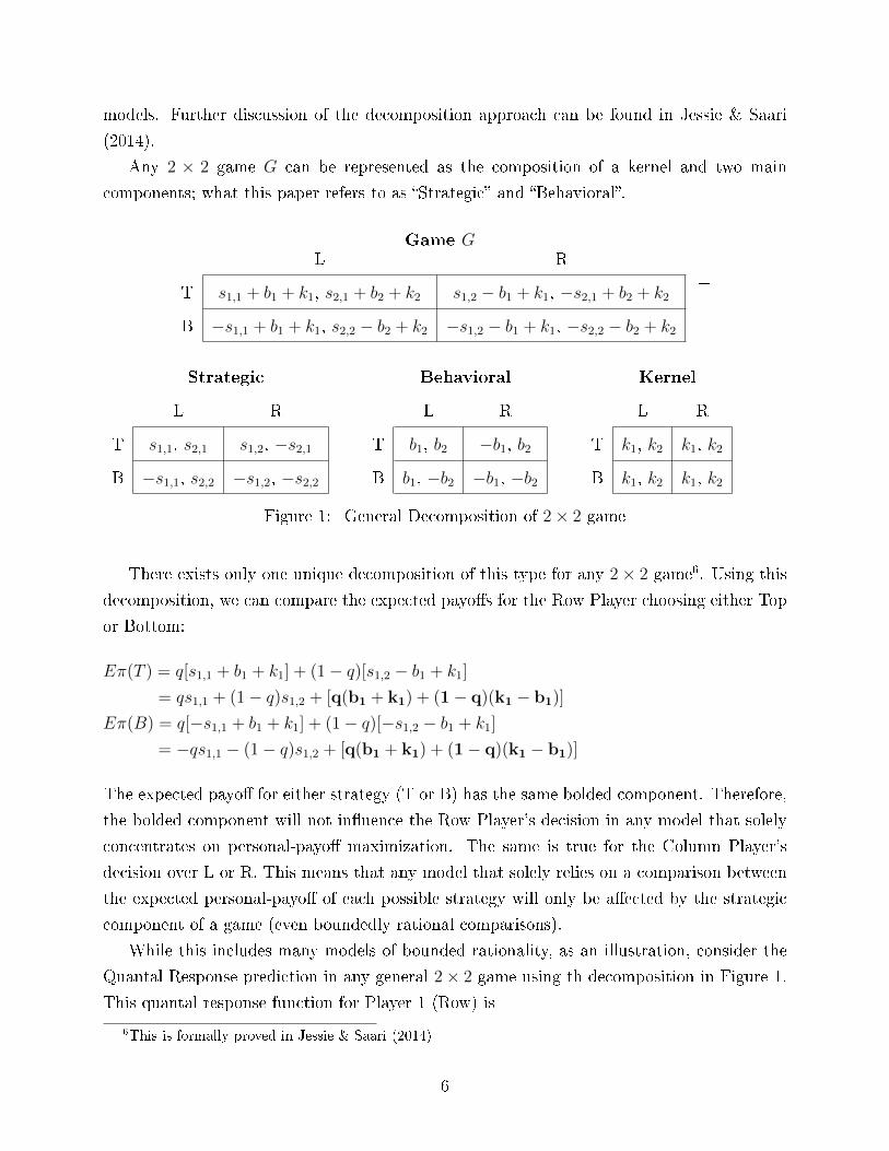
Any 2 × 2 game G can be represented as the composition of a kernel and two main
components; what this paper refers to as �Strategic� and �Behavioral�.
Game GL R
T s1,1 + b1 + k1, s2,1 + b2 + k2 s1,2 − b1 + k1, −s2,1 + b2 + k2
B −s1,1 + b1 + k1, s2,2 − b2 + k2 −s1,2 − b1 + k1, −s2,2 − b2 + k2
=
Strategic
L R
T s1,1, s2,1 s1,2, −s2,1
B −s1,1, s2,2 −s1,2, −s2,2
+
Behavioral
L R
T b1, b2 −b1, b2
B b1, −b2 −b1, −b2
+
Kernel
L R
T k1, k2 k1, k2
B k1, k2 k1, k2
Figure 1: General Decomposition of 2× 2 game
There exists only one unique decomposition of this type for any 2× 2 game6. Using this
decomposition, we can compare the expected payo�s for the Row Player choosing either Top
or Bottom:
Eπ(T ) = q[s1,1 + b1 + k1] + (1− q)[s1,2 − b1 + k1]
= qs1,1 + (1− q)s1,2 + [q(b1 + k1) + (1− q)(k1 − b1)]
Eπ(B) = q[−s1,1 + b1 + k1] + (1− q)[−s1,2 − b1 + k1]
= −qs1,1 − (1− q)s1,2 + [q(b1 + k1) + (1− q)(k1 − b1)]
The expected payo� for either strategy (T or B) has the same bolded component. Therefore,
the bolded component will not in�uence the Row Player's decision in any model that solely
concentrates on personal-payo� maximization. The same is true for the Column Player's
decision over L or R. This means that any model that solely relies on a comparison between
the expected personal-payo� of each possible strategy will only be a�ected by the strategic
component of a game (even boundedly rational comparisons).
While this includes many models of bounded rationality, as an illustration, consider the
Quantal Response prediction in any general 2× 2 game using th decomposition in Figure 1.
This quantal response function for Player 1 (Row) is
6This is formally proved in Jessie & Saari (2014)
6
p1,T = eλE(π̃1,T )
eλE(π̃1,T )+eλE(π̃1,B) .
The expected payo�s can be represented using the decomposed components.
p1,T = eλ(qs1,1+(1−q)s1,2+q(b1+k1)+(1−q)(k1−b1))
eλ(qs1,1+(1−q)s1,2+q(b1+k1)+(1−q)(k1−b1))+eλ(−qs1,1−(1−q)s1,2+q(b1+k1)+(1−q)(k1−b1))
p1,T =(eλ(q(b1+k1)+(1−q)(k1−b1))
eλ(q(b1+k1)+(1−q)(k1−b1))
)eλ(qs1,1+(1−q)s1,2)
eλ(qs1,1+(1−q)s1,2)+eλ(−qs1,1−(1−q)s1,2)
p1,T =eλ(qs1,1+(1−q)s1,2)
eλ(qs1,1+(1−q)s1,2) + eλ(−qs1,1−(1−q)s1,2)(4)
Equation 4 represents a general quantal response function for Player 1 in any 2 × 2 game
using the decomposition7. Notice that the Behavioral (and Kernel) direction cancels out and
only the Strategic component is used to determine the QRE prediction. Therefore, it is not
only the equilibrium prediction, but the entire quantal response function is unresponsive to
changes in the Behavioral component. Because of this, our results using the decomposition
will have the same e�ect on models with homogeneous λs (QRE), heterogeneous λs (HQRE
and ALE), and incorrect beliefs about opponent-play (NI and TQRE).
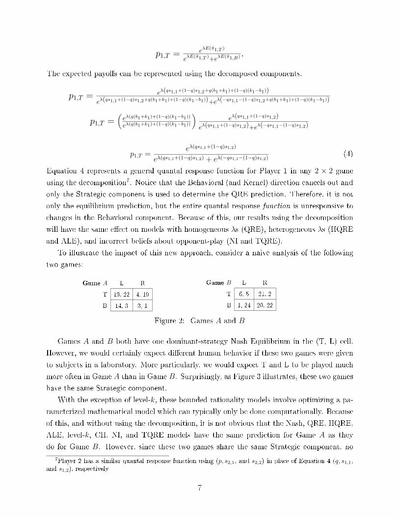
To illustrate the impact of this new approach, consider a naive analysis of the following
two games:
Game A L R
T 19, 22 4, 19
B 14, 3 3, 1
Game B L R
T 6, 5 21, 2
B 1, 24 20, 22
Figure 2: Games A and B
Games A and B both have one dominant-strategy Nash Equilibrium in the (T, L) cell.
However, we would certainly expect di�erent human behavior if these two games were given
to subjects in a laboratory. More particularly, we would expect T and L to be played much
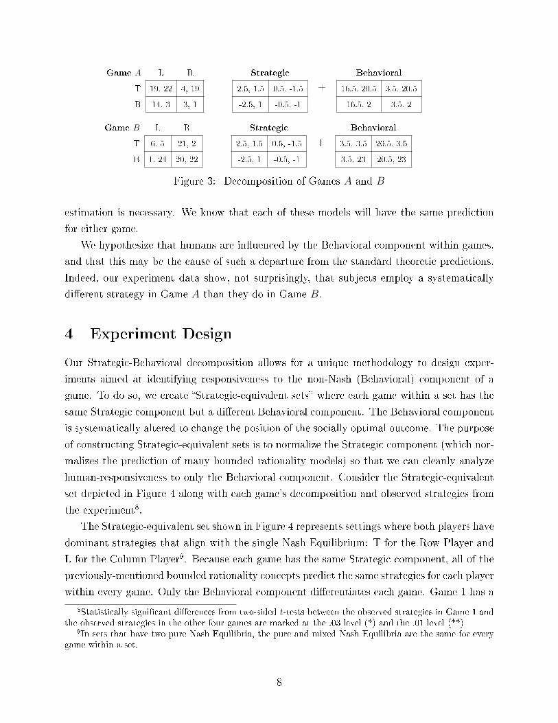
more often in Game A than in Game B. Surprisingly, as Figure 3 illustrates, these two games
have the same Strategic component.
With the exception of level-k, these bounded rationality models involve optimizing a pa-
rameterized mathematical model which can typically only be done computationally. Because
of this, and without using the decomposition, it is not obvious that the Nash, QRE, HQRE,
ALE, level-k, CH, NI, and TQRE models have the same prediction for Game A as they
do for Game B. However, since these two games share the same Strategic component, no
7Player 2 has a similar quantal response function using (p, s2,1, and s2,2) in place of Equation 4 (q, s1,1,and s1,2), respectively
7
Game A L R
T 19, 22 4, 19
B 14, 3 3, 1
=
Strategic
2.5, 1.5 0.5, -1.5
-2.5, 1 -0.5, -1
+
Behavioral
16.5, 20.5 3.5, 20.5
16.5, 2 3.5, 2
Game B L R
T 6, 5 21, 2
B 1, 24 20, 22
=
Strategic
2.5, 1.5 0.5, -1.5
-2.5, 1 -0.5, -1
+
Behavioral
3.5, 3.5 20.5, 3.5
3.5, 23 20.5, 23
Figure 3: Decomposition of Games A and B
estimation is necessary. We know that each of these models will have the same prediction
for either game.
We hypothesize that humans are in�uenced by the Behavioral component within games,
and that this may be the cause of such a departure from the standard theoretic predictions.
Indeed, our experiment data show, not surprisingly, that subjects employ a systematically
di�erent strategy in Game A than they do in Game B.
4 Experiment Design
Our Strategic-Behavioral decomposition allows for a unique methodology to design exper-
iments aimed at identifying responsiveness to the non-Nash (Behavioral) component of a
game. To do so, we create �Strategic-equivalent sets� where each game within a set has the
same Strategic component but a di�erent Behavioral component. The Behavioral component
is systematically altered to change the position of the socially optimal outcome. The purpose
of constructing Strategic-equivalent sets is to normalize the Strategic component (which nor-
malizes the prediction of many bounded rationality models) so that we can cleanly analyze
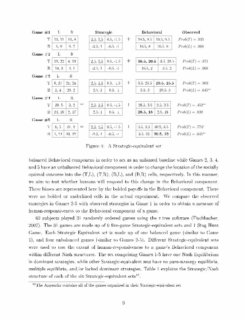
human-responsiveness to only the Behavioral component. Consider the Strategic-equivalent
set depicted in Figure 4 along with each game's decomposition and observed strategies from
the experiment8.
The Strategic-equivalent set shown in Figure 4 represents settings where both players have
dominant strategies that align with the single Nash Equilibrium: T for the Row Player and
L for the Column Player9. Because each game has the same Strategic component, all of the
previously-mentioned bounded rationality concepts predict the same strategies for each player
within every game. Only the Behavioral component di�erentiates each game. Game 1 has a
8Statistically signi�cant di�erences from two-sided t-tests between the observed strategies in Game 1 andthe observed strategies in the other four games are marked at the .03 level (*) and the .01 level (**)
9In sets that have two pure Nash Equilibria, the pure and mixed Nash Equilibria are the same for everygame within a set.
8
Game #1 L R
T 13, 11 10, 8
B 8, 9 9, 7
=
Strategic
2.5, 1.5 0.5, -1.5
-2.5, 1 -0.5, -1
+
Behavioral
10.5, 9.5 10.5, 9.5
10.5, 8 10.5, 8
Observed
Prob(T ) = .935
Prob(L) = .968
Game #2 L R
T 19, 22 4, 19
B 14, 3 3, 1
= 2.5, 1.5 0.5, -1.5
-2.5, 1 -0.5, -1
+ 16.5, 20.5 3.5, 20.5
16.5, 2 3.5, 2
Prob(T ) = .871
Prob(L) = .968
Game #3 L R
T 6, 27 21, 24
B 1, 4 20, 2
= 2.5, 1.5 0.5, -1.5
-2.5, 1 -0.5, -1
+ 3.5, 25.5 20.5, 25.5
3.5, 3 20.5, 3
Prob(T ) = .903
Prob(L) = .645∗∗
Game #4 L R
T 29, 5 3, 2
B 24, 19 2, 17
= 2.5, 1.5 0.5, -1.5
-2.5, 1 -0.5, -1
+ 26.5, 3.5 2.5, 3.5
26.5, 18 2.5, 18
Prob(T ) = .452∗∗
Prob(L) = .839
Game #5 L R
T 6, 5 21, 2
B 1, 24 20, 22
= 2.5, 1.5 0.5, -1.5
-2.5, 1 -0.5, -1
+ 3.5, 3.5 20.5, 3.5
3.5, 23 20.5, 23
Prob(T ) = .774∗
Prob(L) = .645∗∗
Figure 4: A Strategic-equivalent set
balanced Behavioral component in order to act as an unbiased baseline while Games 2, 3, 4,
and 5 have an unbalanced Behavioral component in order to change the location of the socially
optimal outcome into the (T,L), (T,R), (B,L), and (B,R) cells, respectively. In this manner,
we aim to test whether humans will respond to this change in the Behavioral component.
These biases are represented here by the bolded payo�s in the Behavioral component. There
were no bolded or underlined cells in the actual experiment. We compare the observed
strategies in Games 2-5 with observed strategies in Game 1 in order to obtain a measure of
human-responsiveness to the Behavioral component of a game.
62 subjects played 31 randomly ordered games using the z-tree software (Fischbacher,
2007). The 31 games are made up of 6 �ve-game Strategic-equivalent sets and 1 Stag Hunt
Game. Each Strategic Equivalent set is made up of one balanced game (similar to Game
1), and four unbalanced games (similar to Games 2-5). Di�erent Strategic-equivalent sets
were used to test the extent of human-responsiveness to a game's Behavioral component
within di�erent Nash structures. The set comprising Games 1-5 have one Nash Equilibrium
in dominant strategies, while other Strategic-equivalent sets have no pure-strategy equilibria,
multiple equilibria, and/or lacked dominant strategies. Table 1 explains the Strategic/Nash
structure of each of the six Strategic-equivalent sets10.
10The Appendix contains all of the games organized in their Strategic-equivalent set
9

Set Games N.E. count Type of games1 1-5 1 pure Dominant strategies for both players at (T, L)2 6-10 1 pure Dominant strategies for both players at (T, R)3 11-15 2 pure; 1 mixed Battle of Sexes at (T, L) and (B, R)4 16-20 2 pure; 1 mixed Battle of Sexes at (T, R) and (B, L)5 21-25 1 mixed Matching Pennies6 26-30 1 pure Dominant strategies for one player
Table 1: Explanation of Strategic-equivalent sets
Feedback was not provided until all 31 games were played. This was done so that subjects
should not be expected to develop di�erent strategies as the experiment progresses because
of learning or coordination e�ects.
5 Results
5.1 Bounded Rationality
Data from the laboratory experiment support the hypothesis that subjects systematically
respond the the Behavioral Component within a game. Table 2 displays p-values for two-
sided t-tests testing for statistical di�erence between the observed strategies of each game
within the Strategic-equivalent set presented in Figure 4.
Game #2 Game #3 Game #4 Game #5Game Pr(T ) Pr(L) Pr(T ) Pr(L) Pr(T ) Pr(L) Pr(T ) Pr(L)#1 obs. .871 .968 .903 .645 .452 .839 .774 .645
Pr(T ) .935 .4232 - .6621 - .0001∗∗ - .0227∗ -
Pr(L) .968 - 1.00 - .0007∗∗ - .0435 - .0007∗∗
Table 2: Observed responsiveness to Behavioral componentTable 2. Tests for statistical di�erence between the strategies observed in Game 1 and the strategies observedin Games 2, 3, 4, and 5. Numbers represent p-values for two-sided t-tests. Statistically signi�cant di�erencesfrom two-sided t-tests between the observed strategies in Game 1 and the observed strategies in the otherfour games are marked at the .03 level (*) and the .01 level (**) in Table 2, Figure 4, and all �gures in theAppendix.
While the Behavioral component in Game 2 is unbalanced, it is unbalanced in the direction
that reinforces the Nash Equilibrium at TL. There is no con�ict between the Nash Equilibrium
(Strategic component) and the socially optimal outcome (Behavioral component). Because
of this, subjects are not expected to behave di�erently between Game 1 and Game 2. Indeed,
the strategies observed in Game 2 are not statistically di�erent from the observed strategies
10

in Game 1. The Behavioral component in Games 3, 4, and 5 were designed to in�uence a
subject's decision away from the Nash Equilibrium in the TL cell. In Game 3, if the subjects
were in�uenced by the change in the socially optimal outcome (through a change in the
Behavioral component), then Column's strategy would favor R more often than he/she does
in Game 1. This behavior is observed as .645 is statistically lower than .968. Using the
same approach for Game 4, Row's strategy should favor B more often than he/she does in
Game 1. This behavior is observed, as .452 is statistically lower than .935. In Game 5, Row
should favor B and the Column Player should favor R more often than they do in Game 1.
Both of these expected strategies are observed as .774 is statistically lower than .935 and
.645 is statistically lower than .968. In addition, the observed behavior in Games 3-5 did
not signi�cantly di�er from behavior in Game 1 in unanticipated directions. Table 2 serves
as experimental evidence that subjects systematically respond to the Behavioral component.
Similarly signi�cant results are observed for the �ve other Strategic-equivalent sets used in
the experiment. Their corresponding decomposition and statistical tests are located in the
Appendix.
The observed changes in human behavior within Strategic-equivalent sets will not be
predicted by the any model in the class of bounded rationality models build around the Nash
concept. While this point could be illustrated using any of the models previously-mentioned,
we focus, here, on the logit-QRE for two reasonss. First,the logit-QRE has been shown to
accurately capture deviations from Nash behavior in many circumstances. Second, with the
exception of level-k and Cognitive Hierarchy, all of the bounded rationality models discussed
in this paper are an extension of the logit-QRE.
It is well-known that the λ parameter in the logit-QRE is not designed to be estimated
over di�erent games. Because of this, we estimate an individual λ for each strategic equiva-
lent set. This is appropriate because, from the point of view of the logit-QRE, all �ve games
within a Strategic-equivalent set are the same11. The six parameter model is estimated us-
ing a maximum likelihood approach. The estimated λ values for Strategic-equivalent sets
{1, 2, 3, 4, 5, and 6} are {.379, .352,−.038, .017,−.005, and .352}, respectively. These param-eters determine the logit-QRE predictions for each game in Figure 5. The y-axis is either
the observed or predicted probability that T is chosen by the Row player (Player 1). The
x-axis represents the 30 di�erent games. The �rst �ve data points represent Games 1-5 in
Figure 4, the next �ve points represent a di�erent Strategic-equivalent set (Games 6-10), and
so on for each of the six Strategic-equivalent sets comprising the 30 total games. Refer to
Table 1 for the Strategic/Nash structure of each Strategic-equivalent set or the Appendix for
11The fact that the logit-QRE only uses the Strategic component of the game is generally shown in Equation4
11
a decomposition of all 30 games.
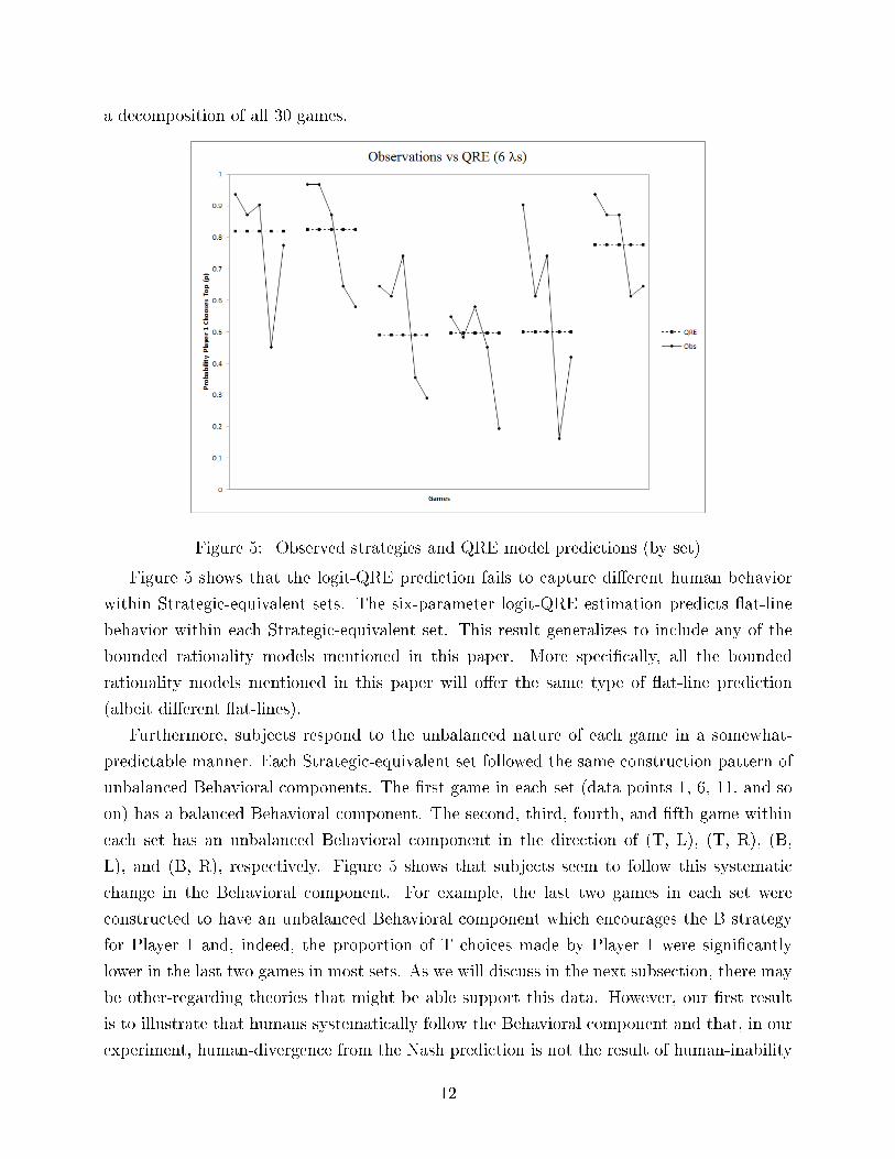
Figure 5: Observed strategies and QRE model predictions (by set)
Figure 5 shows that the logit-QRE prediction fails to capture di�erent human behavior
within Strategic-equivalent sets. The six-parameter logit-QRE estimation predicts �at-line
behavior within each Strategic-equivalent set. This result generalizes to include any of the
bounded rationality models mentioned in this paper. More speci�cally, all the bounded
rationality models mentioned in this paper will o�er the same type of �at-line prediction
(albeit di�erent �at-lines).
Furthermore, subjects respond to the unbalanced nature of each game in a somewhat-
predictable manner. Each Strategic-equivalent set followed the same construction pattern of
unbalanced Behavioral components. The �rst game in each set (data points 1, 6, 11, and so
on) has a balanced Behavioral component. The second, third, fourth, and �fth game within
each set has an unbalanced Behavioral component in the direction of (T, L), (T, R), (B,
L), and (B, R), respectively. Figure 5 shows that subjects seem to follow this systematic
change in the Behavioral component. For example, the last two games in each set were
constructed to have an unbalanced Behavioral component which encourages the B strategy
for Player 1 and, indeed, the proportion of T choices made by Player 1 were signi�cantly
lower in the last two games in most sets. As we will discuss in the next subsection, there may
be other-regarding theories that might be able support this data. However, our �rst result
is to illustrate that humans systematically follow the Behavioral component and that, in our
experiment, human-divergence from the Nash prediction is not the result of human-inability
12
to calculate a statistical generalization of the Nash strategy.
5.2 Other-Regarding Preferences
The Strategic-Behavioral decomposition is designed to normalize the component of a game
concerned with personal-payo� maximization; even bounded-maximization. Of course, this
paper is not the �rst to recognize that humans appear to have more complex preferences than
simple payo�-maximization. The previous literature in this direction has suggested partic-
ular behavioral, or other-regarding, interpretations in order to explain non-Nash behavior.
This section analyzes the experimental data using two well-known other-regarding preference
models of altruism and inequity aversion as well as a novel �corner� preference model.
The bounded rationality models in the previous subsection do not account for human
preferences for altruism or equity. However, these other-regarding preferences have been
shown to accurately �t experimental data and may explain human behavior in our experi-
ment. This is plausible because subjects in our experiment may be motivated to maximize
the payo� they receive because of their action but in addition they also have a preference
for how their choice a�ects the other subject's payo�. To explain the intuition behind these
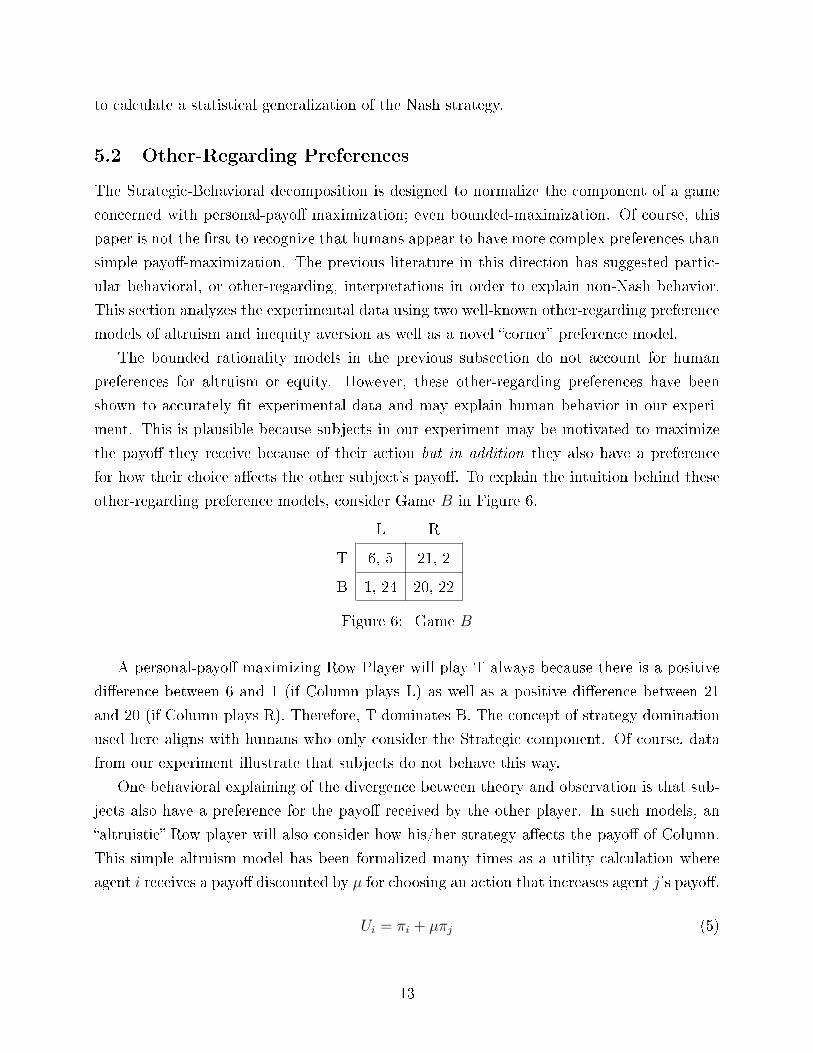
other-regarding preference models, consider Game B in Figure 6.
L R
T 6, 5 21, 2
B 1, 24 20, 22
Figure 6: Game B
A personal-payo� maximizing Row Player will play T always because there is a positive
di�erence between 6 and 1 (if Column plays L) as well as a positive di�erence between 21
and 20 (if Column plays R). Therefore, T dominates B. The concept of strategy domination
used here aligns with humans who only consider the Strategic component. Of course, data
from our experiment illustrate that subjects do not behave this way.
One behavioral explaining of the divergence between theory and observation is that sub-
jects also have a preference for the payo� received by the other player. In such models, an
�altruistic�-Row player will also consider how his/her strategy a�ects the payo� of Column.
This simple altruism model has been formalized many times as a utility calculation where
agent i receives a payo� discounted by µ for choosing an action that increases agent j's payo�.
Ui = πi + µπj (5)
13

Consider altruistic-Row's decision in Game B given that Column plays L. Altruistic-Row's
personal payo� is greater by playing T by a factor of 5 (6-1), but this is counterbalanced by
Column becoming 19 worse o� (5-24) by altruistic-Row's decision to play T instead of B. A
similar counterbalance story holds given that Column plays R. If altruistic-Row is motivated
�su�ciently enough� by the payo� rewarded to Column (if µ is large enough), then he/she
will choose B. Each player's choice is dependent on their preference for altruism, µ. In Game
B, altruistic-Row will choose T if the following inequality holds, and B otherwise.
ERowπ(T ) > ERowπ(B)
q · (πRow,TL + µ · πCol,TL) + (1− q) · (πRow,TR + µ · πCol,TR) >q · (πRow,BL + µ · πCol,BL) + (1− q) · (πRow,BR + µ · πCol,BR)
q · (6 + µ · 5) + (1− q) · (21 + µ · 2) > q · (1 + µ · 24) + (1− q) · (20 + µ · 22) (6)
We model these altruistic players using the same logit-choice model of decision-making. This
generates a model with two estimable parameters that is �tted to our experimental data in
Figure 7.
Figure 7: Observed strategies and altruism model predictions
Because the experiment was speci�cally created to isolate the prediction of bounded
rationality models, it is not surprising to observe that the altruistic model �t the data better
than the logit-QRE (or, likely any other bounded rationality model). The superior �t of
the altruism model is observed between Figure 5 and Figure 7. In addition, the Akaike
14
Information Criterion corrected for �nite sample size suggests that the altruistic model �ts
the data better than the logit-QRE: AICc(Altruism) =75.92<90.04 =AICc(logit-QRE)12 .
While Figure 7 suggests that subjects in the lab may have altruistic preferences, consider
another commonly used model where subjects have a preference for equity. In these models,
an �equity�-Row player will have a preference for how his/her strategy a�ects the di�erence
between his payo� and the payo� of Column. Similar to the altruism model, this model of
inequity-aversion has been formalized in a utility calculation where an agent receives a payo�
discounted by either µ1 or µ2 depending on whether or not the inequity is in his respective
favor.
Ui = πi + µ1 ·Max{π1i − π1
j , 0}+ µ2 ·Max{π2i − π2
j , 0} (7)
Consider an equity-Row Player's decision to choose T in Game B given that Column plays
L. Equity-Row would take into account that Row's personal payo� is greater by playing T
by a factor of 5 (6-1). In addition, T reduces the inequity between the two players because
the di�erence between 1 and 24 is greater than the di�erence between 6 and 5. Also notice
that choosing T or B will change what play the inequity favors. A similar comparison is used
given that Column plays R. The choice made by equity-Row may depend on how strong his
preference is for the equity of payo�s. In Game B, equity-Row will choose T if the following
inequality holds, and B otherwise.
ERowπ(T ) > ERowπ(B)
q · (πRow,TL + µ1 ·Max{πRow,TL − πCol,TL, 0}+ µ2 ·Max{πCol,TL − πRow,TL, 0}) + (1− q) ·(πRow,TR + µ1 ·Max{πRow,TR − πCol,TR, 0}+ µ2 ·Max{πCol,TR − πRow,TR, 0}) >
q · (πRow,BL + µ1 ·Max{πRow,BL − πCol,BL, 0}+ µ2 ·Max{πCol,BL − πRow,BL, 0}) + (1− q) ·(πRow,BR + µ1 ·Max{πRow,BR − πCol,BR, 0}+ µ2 ·Max{πCol,BR − πRow,BR, 0})
q · (6 + µ1 ·Max{6− 5, 0}+ µ2 ·Max{5− 6, 0})) + (1− q) · (21 + µ1 ·Max{21− 2, 0}+ µ2 ·Max{2− 21, 0})) > q · (1 + µ1 ·Max{1− 24, 0}+ µ2 ·Max{24− 1, 0})) + (1− q) · (20 + µ1 ·
Max{20− 22, 0}+ µ2 ·Max{22− 20, 0}))q · (6 + µ1 · 1) + (1− q) · (21 + µ1 · 19) > q · (1 + µ2 · 23) + (1− q) · (20 + µ2 · 2) (8)
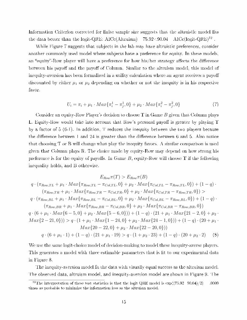
We use the same logit-choice model of decision-making to model these inequity-averse players.
This generates a model with three estimable parameters that is �t to our experimental data
in Figure 8.
The inequity-aversion model �t the data with visually equal success as the altruism model.
The observed data, altruism model, and inequity-aversion model are shown in Figure 9. The
12The interpretation of these test statistics is that the logit-QRE model is exp((75.92=90.04)/2) = .0009times as probable to minimize the information loss as the altruism model.
15
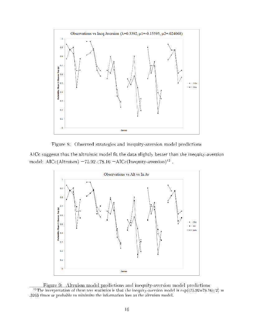
Figure 8: Observed strategies and inequity-aversion model predictions
AICc suggests that the altruistic model �t the data slightly better than the inequity-aversion
model: AICc(Altruism) =75.92<78.16 =AICc(Inequity-aversion)13 .
Figure 9: Altruism model predictions and inequity-aversion model predictions13The interpretation of these test statistics is that the inequity-aversion model is exp((75.92=78.16)/2) =
.3263 times as probable to minimize the information loss as the altruism model.
16
Consider a di�erent model introduced in this paper where agents have a preference for
the corner payo�s in a 2 × 2 game. In this new �corner� model, agents have a preference
over the payo� di�erences between their payo� in a cell and the other agent's payo� in the
opposite corner-cell of the 2 × 2 matrix. There is no reason to expect that humans would
have such a preference, and we anticipate that this nonsensical model will not �t the data
well. However, we formalize this corner model in a utility calculation similar to the altruism
model and inequity-aversion model.
Ui = πi + µπcorner (9)
Consider a �corner�-Row player's decision given that Column chooses L using Game B.
Row's personal payo� is greater by playing T by a factor of 5 (6-1), but this is counterbalanced
by considering the di�erence between the 6 earned by Row in the (T, L) corner cell and the
22 earned by Column in the (B, R) corner cell. A similar comparison is used given that
Column plays R. The choice made by corner-Row depends on how strong his preference is
over the di�erence in the payo�s of the corner cells. In Game B, corner-Row will choose T
if the following inequality holds, and B otherwise.
ERowπ(T ) > ERowπ(B)
q · (πRow,TL + µ · πRow,TL) + (1− q) · (πRow,TR + µ · πRow,TR) >q · (πRow,BL + µ · πCol,BR) + (1− q) · (πRow,BR + µ · πCol,BL)
q · (6 + µ · 6) + (1− q) · (21 + µ · 21) > q · (1 + µ · 22) + (1− q) · (20 + µ · 24) (10)
Of course, the comparison between one player's payo� in a cell with the other player's
payo� in the corner cell should have no in�uence on anyone's choice. There is no reasonable
story as to why a human would compare these numbers. Not only is there a lacking plau-
sible story, but Row player's choice is comprised of nonsensical comparisons (as is Column
player's choice). Therefore, we should expect that a model of corner-bias agents will produce
poor prediction. This model is formalized similarly to the altruistic and inequity-averse mod-
els with a logistic error structure and a two-parameter estimable model with µ measuring
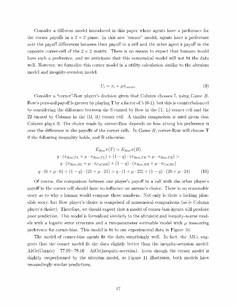
preference for corner-bias. This model is �t to our experimental data in Figure 10.
The model of corner-bias agents �t the data surprisingly well. In fact, the AICc sug-
gests that the corner model �t the data slightly better than the inequity-aversion model:
AICc(Corner) =77.99<78.16 =AICc(Inequity-aversion). Even though the corner model is
slightly outperformed by the altruism model, as Figure 11 illustrates, both models have
resoundingly similar predictions.
17
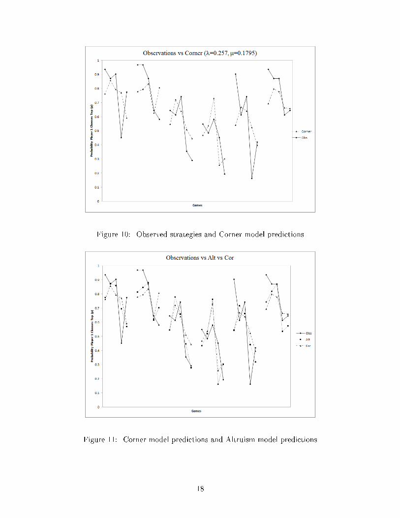
Figure 10: Observed strategies and Corner model predictions
Figure 11: Corner model predictions and Altruism model predictions
18
Fitting models to our experimental data suggests that subjects in our experiment appear
to be equally as altruistic as they are inequity averse as they are corner-bias. Of course,
we hesitate to promote that any of these are the correct behavioral interpretation of human
preferences (especially the nonsensical corner model). However, the fact that the corner model
�ts as well as the two traditional models is concerning for the meaningful interpretation of
any of these models.
6 Conclusion
This paper �nds experimental results suggesting that humans behave di�erently in simple
2×2 games than is predicted by contemporary bounded rationality models. To do so, we use
a laboratory experiment to illustrate a systematic divergence between human-responsiveness
in 2×2 games and a large class of bounded rationality models (Figure 5). This result suggeststhat subjects are in�uenced by our characterization of a game's Behavioral component, which
we o�er as a possible explanation for when and why these models of bounded rationality fail
to provide accurate predictions. The Behavioral component is ignored by these concepts even
though subjects are shown to be responsive to it. When the Behavioral component creates
a tension with the game's Nash structure (Strategic component), these models should be
expected to perform poorly.
Our second result suggests that other-regarding explanations can �t the experimental data
much better than personal-payo� maximizing models. However, in our experiment, we show
that they may lead to spurious and misleading conclusions about the motivations behind
human choices. This is shown in Figure 11 where the prediction o�ered by a classical model
of human-altruism looks very similar to a prediction o�ered by a nonsensical corner-biased
model.
While this paper's results suggest that subjects are in�uenced by the Behavioral compo-
nent, further work is required in order to determine the system of how subjects are in�uenced
by it. Instead of relying upon appropriate sounding stories to generate theories about other-
regarding preferences, the decomposition allows us to formulate theories and predictions using
only the mathematical structures of a game. Future extensions of this project are focused on
developing ex-ante prediction models based on the Strategic-Behavioral decomposition as well
as other decompositions. In addition, the decomposition can be a tool used to normalize the
Strategic component in games which allows for a clean measurement of human-responsiveness
to other traits of interest.
19
Appendix: Further Application - Computing E�ciency
We can utilize our Strategic-Behavioral decomposition to make a signi�cant contribution
to the e�orts focused on creating time-saving logit-QRE-algorithms. Indeed logit-QRE-
algorithms are being implemented to thwart terrorist attacks on America's airport infras-
tructure (ARMOR - Pita, et al., 2008), terminals (GUARDS - Pita, et al., 2011), airplane
�ights (IRIS - Tsai, et al., 2009), as well as attacks on sea ports across the country (PRO-
TECT - An, et al., 2012) to protect natural resources (ARMOR-FOREST - Johnson, et.
al., 2012). The most common problem with applying these logit-QRE-algorithms in the real
world is the extraordinary computing time that the algorithms require.
The Strategic-Behavior decomposition illustrates that the logit-QRE is only sensitive to a
portion of the game. We exploit this fact in order to illustrate that using our decomposition
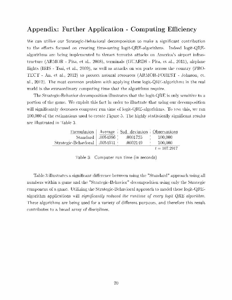
will signi�cantly decreases computer run time of logit-QRE-algorithms. To test this, we ran
100,000 of the estimations used to create Figure 5. The highly statistically signi�cant results
are illustrated in Table 3.
Formulation Average Std. deviation ObservationsStandard .0054986 .0001725 100,000
Strategic-Behavioral .0054051 .0002149 100,000t = 107.2917
Table 3: Computer run time (in seconds)
Table 3 illustrates a signi�cant di�erence between using the "Standard" approach using all
numbers within a game and the "Strategic-Behavior" decomposition using only the Strategic
component of a game. Utilizing the Strategic-Behavioral approach to model these logit-QRE-
algorithm applications will signi�cantly reduced the runtime of every logit-QRE-algorithm.
These algorithms are being used for a variety of di�erent purposes, and therefore this result
contributes to a broad array of disciplines.
20
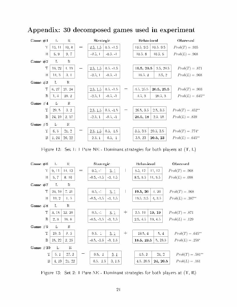
Appendix: 30 decomposed games used in experiment
Game #1 L R
T 13, 11 10, 8
B 8, 9 9, 7
=
Strategic
2.5, 1.5 0.5, -1.5
-2.5, 1 -0.5, -1
+
Behavioral
10.5, 9.5 10.5, 9.5
10.5, 8 10.5, 8
Observed
Prob(T ) = .935
Prob(L) = .968
Game #2 L R
T 19, 22 4, 19
B 14, 3 3, 1
= 2.5, 1.5 0.5, -1.5
-2.5, 1 -0.5, -1
+ 16.5, 20.5 3.5, 20.5
16.5, 2 3.5, 2
Prob(T ) = .871
Prob(L) = .968
Game #3 L R
T 6, 27 21, 24
B 1, 4 20, 2
= 2.5, 1.5 0.5, -1.5
-2.5, 1 -0.5, -1
+ 3.5, 25.5 20.5, 25.5
3.5, 3 20.5, 3
Prob(T ) = .903
Prob(L) = .645∗∗
Game #4 L R
T 29, 5 3, 2
B 24, 19 2, 17
= 2.5, 1.5 0.5, -1.5
-2.5, 1 -0.5, -1
+ 26.5, 3.5 2.5, 3.5
26.5, 18 2.5, 18
Prob(T ) = .452∗∗
Prob(L) = .839
Game #5 L R
T 6, 5 21, 2
B 1, 24 20, 22
= 2.5, 1.5 0.5, -1.5
-2.5, 1 -0.5, -1
+ 3.5, 3.5 20.5, 3.5
3.5, 23 20.5, 23
Prob(T ) = .774∗
Prob(L) = .645∗∗
Figure 12: Set 1: 1 Pure NE - Dominant strategies for both players at (T, L)
Game #6 L R
T 9, 11 14, 13
B 8, 7 8, 10
=
Strategic
0.5, -1 3, 1
-0.5, -1.5 -3, 1.5
+
Behavioral
8.5, 12 11, 12
8.5, 8.5 11, 8.5
Observed
Prob(T ) = .968
Prob(L) = .098
Game #7 L R
T 20, 19 7, 21
B 19, 2 1, 5
= 0.5, -1 3, 1
-0.5, -1.5 -3, 1.5
+ 19.5, 20 4, 20
19.5, 3.5 4, 3.5
Prob(T ) = .968
Prob(L) = .387∗∗
Game #8 L R
T 3, 18 22, 20
B 2, 3 16, 6
= 0.5, -1 3, 1
-0.5, -1.5 -3, 1.5
+ 2.5, 19 19, 19
2.5, 4.5 19, 4.5
Prob(T ) = .871
Prob(L) = .129
Game #9 L R
T 19, 3 8, 5
B 18, 22 2, 25
= 0.5, -1 3, 1
-0.5, -1.5 -3, 1.5
+ 18.5, 4 5, 4
18.5, 23.5 5, 23.5
Prob(T ) = .645∗∗
Prob(L) = .258∗
Game #10 L R
T 5, 1 27, 3
B 4, 19 21, 22
= 0.5, -1 3, 1
-0.5, -1.5 -3, 1.5
+ 4.5, 2 24, 2
4.5, 20.5 24, 20.5
Prob(T ) = .581∗∗
Prob(L) = .161
Figure 13: Set 2: 1 Pure NE - Dominant strategies for both players at (T, R)
21
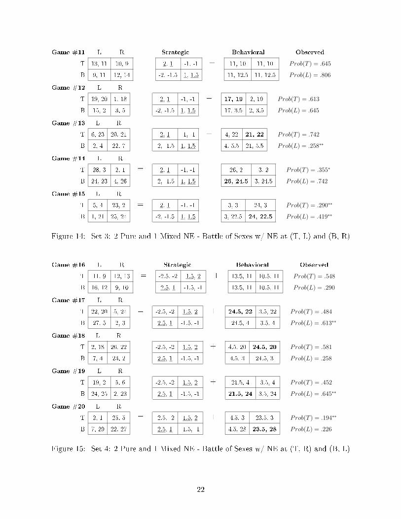
Game #11 L R
T 13, 11 10, 9
B 9, 11 12, 14
=
Strategic
2, 1 -1, -1
-2, -1.5 1, 1.5
+
Behavioral
11, 10 11, 10
11, 12.5 11, 12.5
Observed
Prob(T ) = .645
Prob(L) = .806
Game #12 L R
T 19, 20 1, 18
B 15, 2 3, 5
= 2, 1 -1, -1
-2, -1.5 1, 1.5
+ 17, 19 2, 19
17, 3.5 2, 3.5
Prob(T ) = .613
Prob(L) = .645
Game #13 L R
T 6, 23 20, 21
B 2, 4 22, 7
= 2, 1 -1, -1
-2, -1.5 1, 1.5
+ 4, 22 21, 22
4, 5.5 21, 5.5
Prob(T ) = .742
Prob(L) = .258∗∗
Game #14 L R
T 28, 3 2, 1
B 24, 23 4, 26
= 2, 1 -1, -1
-2, -1.5 1, 1.5
+ 26, 2 3, 2
26, 24.5 3, 24.5
Prob(T ) = .355∗
Prob(L) = .742
Game #15 L R
T 5, 4 23, 2
B 1, 21 25, 24
= 2, 1 -1, -1
-2, -1.5 1, 1.5
+ 3, 3 24, 3
3, 22.5 24, 22.5
Prob(T ) = .290∗∗
Prob(L) = .419∗∗
Figure 14: Set 3: 2 Pure and 1 Mixed NE - Battle of Sexes w/ NE at (T, L) and (B, R)
Game #16 L R
T 11, 9 12, 13
B 16, 12 9, 10
=
Strategic
-2.5, -2 1.5, 2
2.5, 1 -1.5, -1
+
Behavioral
13.5, 11 10.5, 11
13.5, 11 10.5, 11
Observed
Prob(T ) = .548
Prob(L) = .290
Game #17 L R
T 22, 20 5, 24
B 27, 5 2, 3
= -2.5, -2 1.5, 2
2.5, 1 -1.5, -1
+ 24.5, 22 3.5, 22
24.5, 4 3.5, 4
Prob(T ) = .484
Prob(L) = .613∗∗
Game #18 L R
T 2, 18 26, 22
B 7, 4 23, 2
= -2.5, -2 1.5, 2
2.5, 1 -1.5, -1
+ 4.5, 20 24.5, 20
4.5, 3 24.5, 3
Prob(T ) = .581
Prob(L) = .258
Game #19 L R
T 19, 2 5, 6
B 24, 25 2, 23
= -2.5, -2 1.5, 2
2.5, 1 -1.5, -1
+ 21.5, 4 3.5, 4
21.5, 24 3.5, 24
Prob(T ) = .452
Prob(L) = .645∗∗
Game #20 L R
T 2, 1 25, 5
B 7, 29 22, 27
= -2.5, -2 1.5, 2
2.5, 1 -1.5, -1
+ 4.5, 3 23.5, 3
4.5, 28 23.5, 28
Prob(T ) = .194∗∗
Prob(L) = .226
Figure 15: Set 4: 2 Pure and 1 Mixed NE - Battle of Sexes w/ NE at (T, R) and (B, L)
22
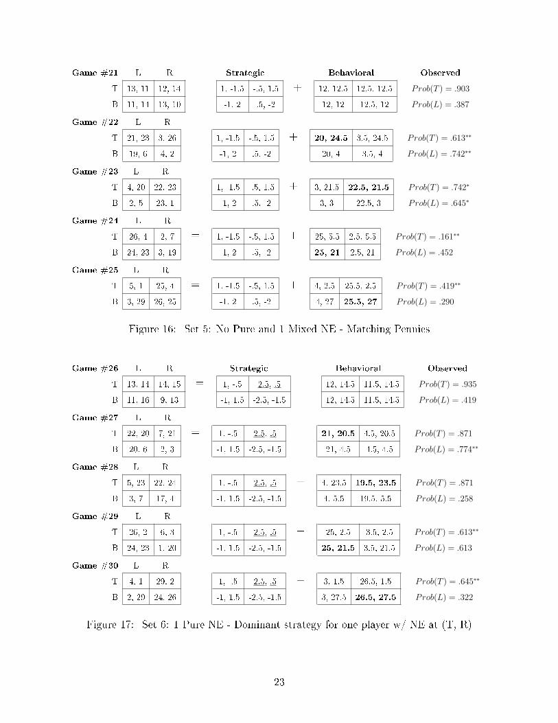
Game #21 L R
T 13, 11 12, 14
B 11, 14 13, 10
=
Strategic
1, -1.5 -.5, 1.5
-1, 2 .5, -2
+
Behavioral
12, 12.5 12.5, 12.5
12, 12 12.5, 12
Observed
Prob(T ) = .903
Prob(L) = .387
Game #22 L R
T 21, 23 3, 26
B 19, 6 4, 2
= 1, -1.5 -.5, 1.5
-1, 2 .5, -2
+ 20, 24.5 3.5, 24.5
20, 4 3.5, 4
Prob(T ) = .613∗∗
Prob(L) = .742∗∗
Game #23 L R
T 4, 20 22, 23
B 2, 5 23, 1
= 1, -1.5 -.5, 1.5
-1, 2 .5, -2
+ 3, 21.5 22.5, 21.5
3, 3 22.5, 3
Prob(T ) = .742∗
Prob(L) = .645∗
Game #24 L R
T 26, 4 2, 7
B 24, 23 3, 19
= 1, -1.5 -.5, 1.5
-1, 2 .5, -2
+ 25, 5.5 2.5, 5.5
25, 21 2.5, 21
Prob(T ) = .161∗∗
Prob(L) = .452
Game #25 L R
T 5, 1 25, 4
B 3, 29 26, 25
= 1, -1.5 -.5, 1.5
-1, 2 .5, -2
+ 4, 2.5 25.5, 2.5
4, 27 25.5, 27
Prob(T ) = .419∗∗
Prob(L) = .290
Figure 16: Set 5: No Pure and 1 Mixed NE - Matching Pennies
Game #26 L R
T 13, 14 14, 15
B 11, 16 9, 13
=
Strategic
1, -.5 2.5, .5
-1, 1.5 -2.5, -1.5
+
Behavioral
12, 14.5 11.5, 14.5
12, 14.5 11.5, 14.5
Observed
Prob(T ) = .935
Prob(L) = .419
Game #27 L R
T 22, 20 7, 21
B 20, 6 2, 3
= 1, -.5 2.5, .5
-1, 1.5 -2.5, -1.5
+ 21, 20.5 4.5, 20.5
21, 4.5 4.5, 4.5
Prob(T ) = .871
Prob(L) = .774∗∗
Game #28 L R
T 5, 23 22, 24
B 3, 7 17, 4
= 1, -.5 2.5, .5
-1, 1.5 -2.5, -1.5
+ 4, 23.5 19.5, 23.5
4, 5.5 19.5, 5.5
Prob(T ) = .871
Prob(L) = .258
Game #29 L R
T 26, 2 6, 3
B 24, 23 1, 20
= 1, -.5 2.5, .5
-1, 1.5 -2.5, -1.5
+ 25, 2.5 3.5, 2.5
25, 21.5 3.5, 21.5
Prob(T ) = .613∗∗
Prob(L) = .613
Game #30 L R
T 4, 1 29, 2
B 2, 29 24, 26
= 1, -.5 2.5, .5
-1, 1.5 -2.5, -1.5
+ 3, 1.5 26.5, 1.5
3, 27.5 26.5, 27.5
Prob(T ) = .645∗∗
Prob(L) = .322
Figure 17: Set 6: 1 Pure NE - Dominant strategy for one player w/ NE at (T, R)
23

References
[1] Akaike, Hirotugu. 1974. �A new look at the statistical model identi�cation.� Automatic
Control, IEEE Transactions on 19(6): 716-723.
[2] An, Bo, Eric Shieh, Rong Yang, Milind Tambe, Craig Baldwin, Joseph
DiRenzo, Ben Maule, and Garrett Meyer. 2012. �PROTECT: A Deployed
Game Theoretic System to Protect the Ports of the United States�. Proc. of
The 11th Int. Conf. on Autonomous Agents and Multiagent Systems (AAMAS).
http://teamcore.usc.edu/papers/2013/protect_aim.pdf
[3] Andreoni, James . 1990. �Impure Altruism and Donations to Public Goods: A Theory
of Warm Glow Giving.� The Economic Journal, 100: 464 - 477.
[4] Andreoni, James and John Miller. 2002. �Giving According to GARP: An Experi-
mental Test of the Consistency of Preferences for Altruism.� Econometrica, 70(2): 737
- 753.
[5] Bénabou, Roland and Jean Tirole. 2011. �Identity, Morals, and Taboos: Beliefs as
Assets.� The Quarterly Journal of Economics, 126(2): 805-855.
[6] Binmore, Ken and Avner Shaked. 2010. �Experimental Economics: Where Next?�
Journal of Economics Behavior & Organization, 73: 87 - 100.
[7] Brunner, Christopher, Colin Camerer, and Jacob Goeree. 2011. �Stationary
Concepts for Experimental 2 × 2 Games: Comment� American Economic Review, 101:
1029 - 1040.
[8] Camerer, C. F., Ho, T. H., & Chong, J. K. 2004. �A Cognitive Hierarchy Model
of Games.� The Quarterly Journal of Economics, 119(3), 861-898.
[9] Capra, Monica C., Jacob Goeree, Rosario Gomez, and Charles Holt. 1999.
�Anomalous Behavior in a Traveler's Dilemma?� American Economic Review, 89: 678 -
690.
[10] Crawford, V. P., Costa-Gomes, M. A., & Iriberri, N. 2013. �Structural models
of nonequilibrium strategic thinking: Theory, evidence, and applications.� Journal of
Economic Literature, 51(1), 5-62.
[11] Dufwenberg, Martin. and Georg Kirchsteiger. 2004. �A Theory of Sequential
Reciprocity� Games and Economic Behavior, 47: 268 - 298.
24
[12] Fehr, Ernst and Klaus M. Schmidt. 1999. �A Theory of Fairness, Competition, and
Cooperation� Quarterly Journal of Economics, 114(3): 817 - 868.
[13] Fehr, Ernst, Michael Naef, and Klaus M. Schmidt. 2006. �Inequality Aversion,
E�ciency, and Maximin Preferences in Simple Distribution Experiments: Comment.�
American Economic Review, 96(5): 1912-1917.
[14] Fischbacher, Urs. 2007. �Z-Tree: Zurich Toolbox for Read-made Economic Experi-
ments� Experimental Economics, 10: 171-178.
[15] Goeree, Jacob. and Charles Holt. 2004. �A Model of Noisy Introspection� Games
and Economic Behavior, 46(2): 365 - 382.
[16] Goeree, Jacob. and Charles Holt. 2005. �An Experimental Study of Costly Coor-
dination� Games and Economic Behavior, 46(2): 281 - 294.
[17] Ho�man, Elizabeth, Kevin McCabe, and Vernon L. Smith. 1996. �Social Dis-
tance and Other Regarding Behavior in Dictator Games� American Economic Review,
86(3): 653-660.
[18] Hurvich, Cli�ord M. and Chih-Ling Tsai. 1989. �Regression and time series model
selection in small samples.� Biometrika 76(2): 297-307.
[19] Jessie, Daniel and Donald G. Saari. 2013. �The Mathematical Structure and Anal-
ysis of Games� [Working Paper], 2014.
[20] Johnson, Matthew P., Fei Fang, and Milind Tambe 2012. �Patrol Strategies to
Maximize Pristine Forest Area.� in Conference on Arti�cial Intelligence (AAAI), July.
[21] Levine, David K. 1998. �Modeling Altruism and Spitefulness in Experiments� Review
of Economic Dynamics, 1: 593 - 622.
[22] Levine, David K. and Thomas R. Palfrey. 2007. �The Paradox of Voter Partic-
ipation? A Laboratory Study� The American Political Science Review, 101(1): 143 -
158.
[23] Luce, Duncan. 1959. Individual Choice Behavior. New York, Wesley.
[24] McKelvey, Richard D. and Thomas R. Palfrey. 1995. �Quantal Response Equi-
librium for Normal Form Games� Games and Economic Behavior, 10: 6 - 38.
[25] McKelvey, Richard D. and Thomas R. Palfrey. 1998. �Quantal Response Equi-
librium for Extensive Form Games� Experimental Economics, 1(1): 9 - 41.
25
[26] McKelvey, Richard D., Thomas R. Palfrey, and Roberto A. Weber. 2000. �The
e�ects of payo� magnitude and heterogeneity on behavior in 2 × 2 games with unique
mixed strategy equilibria.� Journal of Economic Behavior & Organization, 42(4): 523-
548.
[27] Nagel, R. 1995. �Unraveling in guessing games: An experimental study.� American
Economic Review, 85(5): 1313-1326.
[28] Nash, John F. 1950. �Equilibrium Points in N-Person Games� Proceedings of the Na-
tional Academy of Sciences, 36: 48 - 49.
[29] Nash, John F. 1951. �Non-Cooperative Games� Annals of Mathematics, 2(54): 286 -
295.
[30] Pita, James, Manish Jain, Janusz Marecki, Fernando Ordonez, Christopher
Portway, Milind Tambe, Craig Western, Praveen Paruchuri, and Sarit Kraus.
2008. �Deployed ARMOR Protection: The Application of a Game Theoretic Model for
Security at the Los Angeles International Airport� Proc. of 7th Int. Conf. on Autonomous
Agents and Multiagent Systems (AAMAS 2008) - Industry and Applications Track.
Berger, Burg, Nishiyama (eds.), May, 12-16, Estoril, Portugal.
[31] Pita, James, Milind Tambe, Chris Kiekintveld, Shane Cullen, and Erin
Steigerwald. 2011. �GUARDS - Game Theoretic Security Allocation on a National
Scale� Proc. of 10th Int. Conf. on Autonomous Agents and Multiagent Systems (AA-
MAS 2011) - Innovative Applications Track. Tumer, Yolum, Sonenberg and Stone (eds.),
May, 2-6, Taipei, Taiwan.
[32] Rabin, Matthew. 1993. �Endogenous Preferences in Games� American Economics
Review, 83: 1281 - 1302.
[33] Rogers, B. W., Palfrey, T. R., & Camerer, C. F. 2009. �Heterogeneous quantal
response equilibrium and cognitive hierarchies.� Journal of Economic Theory, 144(4),
1440-1467.
[34] Selten, Reinhard and Thorsten Chmura. 2008. �Stationary Concepts for Experi-
mental 2 × 2 Games� American Economics Review, 98(3): 938 - 966.
[35] Stahl II, D. O., & Wilson, P. W. 1994. �Experimental evidence on players' models
of other players.� Journal of Economic Behavior & Organization, 25(3): 309-327.
26
[36] Tsai, Jason, Shyamsunder Rathi, Christopher Kiekintveld, Fernando Or-
donez, Milind Tambe. 2009. �IRIS - A Tool for Strategic Security Allocation in
Transportation Networks� Proc. of 8th Int. Conf. on Autonomous Agents and Multi-
agent Systems (AAMAS 2009). Decker, Sichman, Sierra and Castelfranchi (eds.), May,
10-15, Budapest, Hungary.
[37] Weizsäcker, G. 2003. �Ignoring the rationality of others: evidence from experimental
normal-form games.� Games and Economic Behavior, 44(1): 145-171.
27