Embed Size (px)
Citation preview
Decoherence and Programmable Quantum Computation
Jeff P. Barnes and Warren S. Warren
Chemistry Department, Princeton University, Princeton, NJ 08544-1009
(February 26, 1999)
Abstract
An examination of the concept of using classical degrees of freedom to drive the evolution
of quantum computers is given. Specifically, when externally generated, coherent states of
the electromagnetic field are used to drive transitions within the qubit system, a decoher-
ence results due to the back reaction from the qubits onto the quantum field. We derive an
expression for the decoherence rate for two cases, that of the single-qubit Walsh-Hadamard
transform, and for an implementation of the controlled-NOT gate. We examine the impact
of this decoherence mechanism on Grover’s search algorithm, and on the proposals for use of
error-correcting codes in quantum computation.
PACS number(s): 03.67.Lx, 32.80.Qk
1
1 Introduction
In the original concept of quantum computation, the isolated, coherent evolution of a quantum
system corresponded to a series of logical operations which could be used to compute a solution
to a problem [1]. In this concept, once a method of solving a given problem is decided upon,
the logical steps in the method are translated into unitary transforms of a quantum system [2].
These transforms demand a certain form for the Hamiltonian H that describes the evolution of
the quantum computer, which in turn constrains the architecture of the quantum system. In other
words, the program determines the system propagator, U(t) = exp(−iHt/h), which determines the
form of H , whose parameters indicate the qubit-qubit interactions that must be present in order to
carry out the program.
Such quantum computers suffer from a significant drawback: they are not programmable. Con-
sider the case of NMR quantum computing. A given program to solve a given problem determines
H , which in turn determines the magnitudes of the J couplings between distinct spins, which
in turn constrains the geometry of the molecule to be used as the quantum system. Once the
molecule is created, perhaps utilizing organic synthetic chemistry, it is in general useful only for the
method of solving the problem originally decided upon. In contrast with the flexibility of classical,
transistor-based computers, these quantum computers have their programs “hard-wired” into their
architecture.
However, recent proposals for quantum computer architectures seek to overcome this limitation.
2
They use external fields, generated by classical degrees of freedom, in order to drive the quantum
system’s evolution [3]. Since classical sources can easily be manipulated by the (presumably clas-
sical) programmer, these methods offer a means by which the programmer can alter the evolution
of the quantum system, and thus program the computer. Some of these proposals include the
use of radio-frequency pulses acting upon nuclear spins in liquids [4, 5], laser pulses acting upon
ions trapped in resonators [6, 7], electrostatic fields generated from gated electrodes influencing the
evolution of nuclear spins in semiconductors [8], or electrons trapped in quantum dot structures [9].
There is a question that naturally arises when one contemplates such proposals: how can the
evolution of a quantum system remain coherent if it is interacting with classical degrees of freedom?
Consider the loss of visibility of the interference pattern in a two-slit electron beam experiment
which occurs when one attempts to measure which path the electron took using a light source [10].
The interaction of the field with the electron creates an entangled state of the electron and field,
from which a measurement of the state of the light will reveal information about the position of
the electron. To the extent to which the light carries information about which path the electron
takes, interference is lost [10, 11, 12]. Such interference is central to the working of many quantum
programs, e.g. Grover’s search algorithm [13]. If we use classically generated fields to drive (and
thus interact) with the qubits, will that interaction effectively measure the state of the qubits, and
by doing so, destroy the coherent evolution of the system?
To answer this question, we examine a specific case, that of Grover’s quantum search algorithm
3
[13]. First, we review the implementation of this algorithm when quantum back reaction is not a
concern. Then we assume that one of the transforms used in the algorithm, the Walsh-Hadamard
transform, is driven by externally applied electromagnetic pulses. The quantum field is assumed to
be generated by classical sources, so that it is described by a coherent field state. Thus, the quantum
field exhibits behavior that is close to a classical field. Despite this, there is some quantum back-
reaction on the field which leads to a decoherence of the qubit system. We determine the rate of
decoherence due to this process. Finally, we discuss the broader implications of this mechanism of
decoherence. While these questions have been previously raised [14], to the author’s knowledge no
quantitative assessment of their importance has yet been given.
2 Grover’s algorithm
2.1 Discussion
Before we consider how to drive a part of Grover’s search algorithm, let us briefly review it here.
Grover’s quantum search algorithm is a method by which to retrieve elements in a subset of a larger
set [13]. It acts upon K qubits, or two-level systems, whose levels are arbitrarily label as |0〉 and
|1〉. A complete, orthonormal basis for the system is the product basis, e.g. for K=3, |000〉, |001〉,
|010〉, |011〉, |100〉, |101〉, |110〉, |111〉. It is usual to refer to each element of the basis set by the
integer whose binary expansion represents the string of 0s and 1s, so that |3〉 ≡ |011〉. The elements
4
of the set to be searched are labeled by the integers from 0 to 2K − 1.
The subset whose elements we are searching for is specified according to a condition. For
example, we could search for any integer-valued roots of a given polynomials within a fixed range.
There are many problems for which, given an x of the set of possible solutions, it can be checked in
a polynomial number of steps whether x is a solution to the problem, but no known method exists
to find all solutions in polynomial steps [15]. These problems can be solved by a brute-force search
over all possible solutions, which is what Grover’s algorithm does. Since Grover’s algorithm has
been shown to be optimal [16, 17, 18], its performance is one important indicator of how quantum
computation might out-perform classical computation.
In what follows, we assume there is only a single solution, y, to the problem. It is not dif-
ficult to generalize this to multiple solutions [17]. The initial state of the quantum computer is
∑2K−1x=0 |x〉/
√2K . The goal is to transfer amplitude into the state |y〉 [13] so that a measurement of
the system yields the solution. This is achieved by a series of transforms of the form (WRWO)N .
The unitary, Hermitian operator W =∏
nW(n) =∏
n
√2 (Sx(n) - Sz(n)) is the Welsh-Hadamard
transform. It consists of a product of transforms, acting independently on each qubit in the system.
(When referring to a single qubit, we employ the Pauli spin operator notation as commonly used in
magnetic resonance [19]. In particular, Sα = |1〉〈1| and Sβ = |0〉〈0| are projection operators, and
S+ = |1〉〈0| and S− = |0〉〈1| are raising and lowering operators for a single qubit.)
The operators R = −1 + 2|0〉〈0| and O = 1 - 2|y〉〈y| are diagonal in the product basis. The
5
operator O is called the oracle. It is the only means by which the algorithm has knowledge of
the solution. It would be the routine the flips the amplitude of the state |x〉, for example, if
x were the root of a given polynomial. The combination WRW can also be written as −1 +
2(∑2K−1
x=0 |x〉)(∑2K−1x=0 〈x|)/2K , which is called the invert-about-average step.
The algorithm can be understood as a combination of two inversions, the first about |y〉 and
the second about the state with an equal amplitude for all basis states. The two inversions result
in a rotation, transferring amplitude into |y〉 [13, 18]. For any normalized state of the computer,
∑2K−1x=0 ax|x〉, the application of the transformation WRWO alters the state as follows:
ay
∑x 6=y
ax√2K − 1
WRWO−→
1− 2
2K
2
2K
√2K − 1
− 2
2K
√2K − 1 1− 2
2K
ay
∑x 6=y
ax√2K − 1
(1)
which is a rotation of the probability amplitude between |y〉 and all other states, with sinϕ ≈ 21−K/2
for large K. When ay and∑
x 6=y ax have the same sign, the amplitude for the state |y〉 increases
with every iteration, and decreases otherwise.
Note that R and O, unlike W, are not products of operators acting independently upon each
qubit. They require qubit-qubit interactions to implement. To see this, write R = −1 + 2∏
n Sβ(n)
= −1 + 2∏
n[1/2−Sz(n)]. When the product is expanded, terms such as Sz(n)Sz(m) appear, which
indicate the need for qubit interactions.
6
2.2 Adding Classical Fields
Consider how to drive the algorithm utilizing externally applied fields. The Walsh-Hadamard
transforms W(n) can be driven one qubit at a time. Some proposals include methods by which
qubit-qubit couplings, and thus R and O, could also be driven [8, 7]. We assume here that only the
W(n) are externally driven. Because of the nature of decoherence, it is reasonable to expect that
if further transforms besides W(n) are driven, the decoherence rate can only increase from what is
derived below.
Suppose that there exists a field / qubit coupling of the form κE(t)Sx, where E(t) is the
electric field amplitude, and κ is the field / qubit coupling. We assume the field uses only a single
polarization for simplicity. If the qubits are magnetic dipoles, the form of the coupling is unchanged,
with B(t) substituted for E(t). To give our programmer the greatest possible control, it is usually
assumed that each qubit can be separately driven by the field. There are two ways to achieve this:
spatial resolution (as is usually the case for lasers acting upon ions in traps) or frequency resolution
(as is used in magnetic resonance). In either case, the Fourier components of the pulses acting upon
separate qubits do not overlap. If spatial resolution is employed, then to prevent the pulses from
overlapping, different directions of the beams are used. If frequency resolution is employed, then
the pulses are centered at different frequencies in order to select a given transition.
7
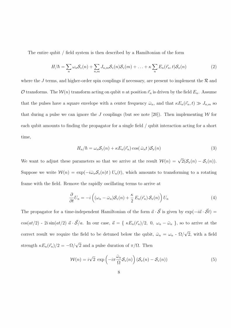
The entire qubit / field system is then described by a Hamiltonian of the form
H/h =∑n
ωnSz(n) +∑n,m
Jn,mSz(n)Sz(m) + . . .+ κ∑n
En(~rn, t)Sx(n) (2)
where the J terms, and higher-order spin couplings if necessary, are present to implement theR and
O transforms. TheW(n) transform acting on qubit n at position ~rn is driven by the field En. Assume
that the pulses have a square envelope with a center frequency ωn, and that κEn(~rn, t) Jn,m so
that during a pulse we can ignore the J couplings (but see note [20]). Then implementing W for
each qubit amounts to finding the propagator for a single field / qubit interaction acting for a short
time,
Hn/h = ωnSz(n) + κEn(~rn) cos( ωnt )Sx(n) (3)
We want to adjust these parameters so that we arrive at the result W(n) =√
2(Sx(n) − Sz(n)).
Suppose we write W(n) = exp(−iωnSz(n)t ) Un(t), which amounts to transforming to a rotating
frame with the field. Remove the rapidly oscillating terms to arrive at
∂
∂tUn = −i
((ωn − ωn)Sz(n) +
κ
2En(~rn)Sx(n)
)Un (4)
The propagator for a time-independent Hamiltonian of the form ~a · ~S is given by exp(−i~a · ~St) =
cos(at/2) - 2i sin(at/2) ~a · ~S/a. In our case, ~a = κEn(~rn)/2, 0, ωn − ωn , so to arrive at the
correct result we require the field to be detuned below the qubit, ωn = ωn - Ω/√
2, with a field
strength κEn(~rn)/2 = −Ω/√
2 and a pulse duration of π/Ω. Then
W(n) = i√
2 exp(−iπ ωn
ΩSz(n)
)(Sx(n)− Sz(n)) (5)
8
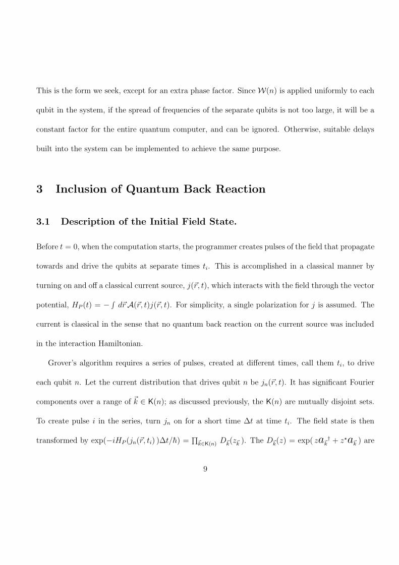
This is the form we seek, except for an extra phase factor. Since W(n) is applied uniformly to each
qubit in the system, if the spread of frequencies of the separate qubits is not too large, it will be a
constant factor for the entire quantum computer, and can be ignored. Otherwise, suitable delays
built into the system can be implemented to achieve the same purpose.
3 Inclusion of Quantum Back Reaction
3.1 Description of the Initial Field State.
Before t = 0, when the computation starts, the programmer creates pulses of the field that propagate
towards and drive the qubits at separate times ti. This is accomplished in a classical manner by
turning on and off a classical current source, j(~r, t), which interacts with the field through the vector
potential, HP (t) = − ∫ d~rA(~r, t)j(~r, t). For simplicity, a single polarization for j is assumed. The
current is classical in the sense that no quantum back reaction on the current source was included
in the interaction Hamiltonian.
Grover’s algorithm requires a series of pulses, created at different times, call them ti, to drive
each qubit n. Let the current distribution that drives qubit n be jn(~r, t). It has significant Fourier
components over a range of ~k ∈ K(n); as discussed previously, the K(n) are mutually disjoint sets.
To create pulse i in the series, turn jn on for a short time ∆t at time ti. The field state is then
transformed by exp(−iHP (jn(~r, ti) )∆t/h) =∏
~k∈K(n) D~k(z~k ). The D~k(z) = exp( za~k† + z?a~k ) are
9
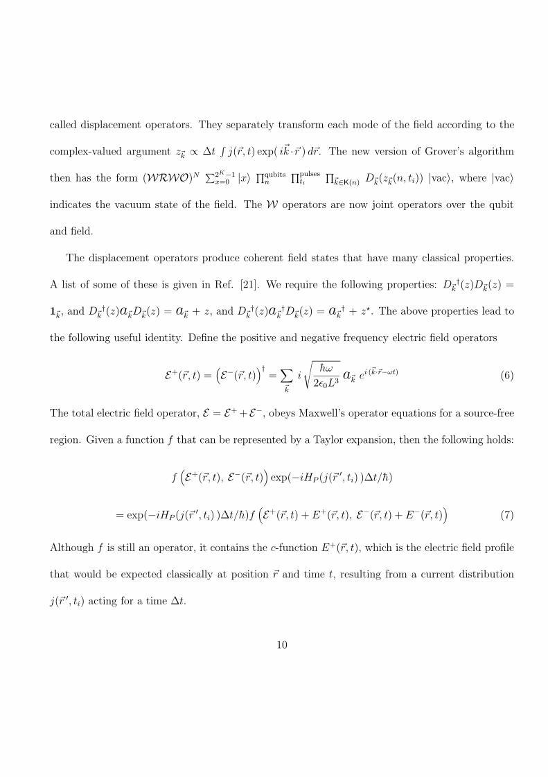
called displacement operators. They separately transform each mode of the field according to the
complex-valued argument z~k ∝ ∆t∫j(~r, t) exp( i~k ·~r ) d~r. The new version of Grover’s algorithm
then has the form (WRWO)N ∑2K−1x=0 |x〉 ∏qubits
n
∏pulsesti
∏~k∈K(n) D~k(z~k(n, ti)) |vac〉, where |vac〉
indicates the vacuum state of the field. The W operators are now joint operators over the qubit
and field.
The displacement operators produce coherent field states that have many classical properties.
A list of some of these is given in Ref. [21]. We require the following properties: D~k†(z)D~k(z) =
1~k, and D~k†(z)a~kD~k(z) = a~k + z, and D~k
†(z)a~k†D~k(z) = a~k
† + z?. The above properties lead to
the following useful identity. Define the positive and negative frequency electric field operators
E+(~r, t) =(E−(~r, t)
)†=∑~k
i
√hω
2ε0L3a~k e
i (~k·~r−ωt) (6)
The total electric field operator, E = E+ +E−, obeys Maxwell’s operator equations for a source-free
region. Given a function f that can be represented by a Taylor expansion, then the following holds:
f(E+(~r, t), E−(~r, t)
)exp(−iHP (j(~r ′, ti) )∆t/h)
= exp(−iHP (j(~r ′, ti) )∆t/h)f(E+(~r, t) + E+(~r, t), E−(~r, t) + E−(~r, t)
)(7)
Although f is still an operator, it contains the c-function E+(~r, t), which is the electric field profile
that would be expected classically at position ~r and time t, resulting from a current distribution
j(~r ′, ti) acting for a time ∆t.
10
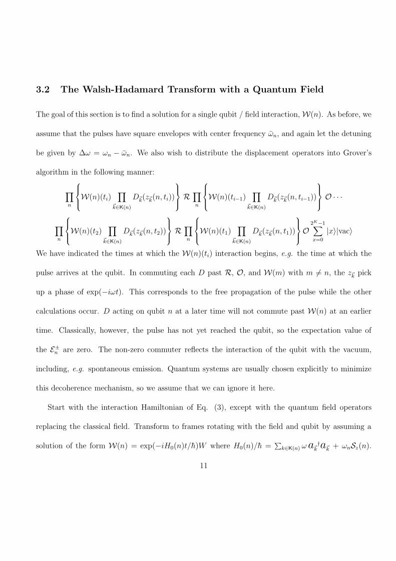
3.2 The Walsh-Hadamard Transform with a Quantum Field
The goal of this section is to find a solution for a single qubit / field interaction, W(n). As before, we
assume that the pulses have square envelopes with center frequency ωn, and again let the detuning
be given by ∆ω = ωn − ωn. We also wish to distribute the displacement operators into Grover’s
algorithm in the following manner:
∏n
W(n)(ti)∏
~k∈K(n)
D~k(z~k(n, ti))
R ∏n
W(n)(ti−1)∏
~k∈K(n)
D~k(z~k(n, ti−1))
O · · ·
∏n
W(n)(t2)∏
~k∈K(n)
D~k(z~k(n, t2))
R ∏n
W(n)(t1)∏
~k∈K(n)
D~k(z~k(n, t1))
O2K−1∑x=0
|x〉|vac〉
We have indicated the times at which the W(n)(ti) interaction begins, e.g. the time at which the
pulse arrives at the qubit. In commuting each D past R, O, and W(m) with m 6= n, the z~k pick
up a phase of exp(−iωt). This corresponds to the free propagation of the pulse while the other
calculations occur. D acting on qubit n at a later time will not commute past W(n) at an earlier
time. Classically, however, the pulse has not yet reached the qubit, so the expectation value of
the E±n are zero. The non-zero commuter reflects the interaction of the qubit with the vacuum,
including, e.g. spontaneous emission. Quantum systems are usually chosen explicitly to minimize
this decoherence mechanism, so we assume that we can ignore it here.
Start with the interaction Hamiltonian of Eq. (3), except with the quantum field operators
replacing the classical field. Transform to frames rotating with the field and qubit by assuming a
solution of the form W(n) = exp(−iH0(n)t/h)W where H0(n)/h =∑
k∈K(n) ωa~k†a~k + ωnSz(n).
11
This results in an equation for W ,
d
dtW (t) = −iκ
2
(S+(n)eiωnt E+
n (~rn, t) + S−(n)e−iωntE−n (~rn, t))W (t) (8)
The modes over K(n) in the operator E±n slowly dephase during the interaction of the pulse with the
qubit. This gives the effect of the pulse envelope on the qubit, but makes a solution somewhat diffi-
cult. However, our interest is to find only the lowest order departures from classical behavior. Here
is one way to do this: first, insert a unit factor into the propagator, exp(−iH0(n)t/h)∏
K(n)D~kD~k†
W (t)∏
K(n)D~k |vac〉. The D to the right commutes to the front of the entire algorithm, and we
solve for U ≡ D†WD instead. From Eq. (7), this results in replacing E±n with E±n +E±n in Eq. (8),
where E±n is the classical field at the qubit.
Two things have changed. First, the appearance of the classical field profiles in Eq. (8) means
that part of U alters the qubit evolution according to the classical field profile. Photons are still
absorbed and emitted by the qubit, but the process occurs in such a way so that the coherent
state of the field is not altered (which is a very “classical” behavior). Second, U still contains field
operators, but now they act upon the vacuum state of the field with the D to the left. U will
create one-photon states (and higher orders as well) which are orthogonal to the vacuum state.
Because D is a unitary transform, the displaced one-photon states are orthogonal to the displaced
vacuum states that describe the pulses. Thus, U can entangle the qubit state with a new field state
orthogonal to the original field state. This is precisely the description of a decoherence mechanism.
The idea that the classical field represents the lowest-order behavior suggests we should expand
12
out U as a series,∑
j Uj , for which j corresponds to the power of the quantum field operators (or
equivalently, the power of√h). This results in
d
dtU0 = −iκ
2
(E+
n S+(n)eiωnt + E−n S−(n)e−iωnt)U0
for the classical behavior, and for j ≥ 1,
d
dtUj = −iκ
2
(E+
n S+(n)eiωnt + E−n S−(n)e−iωnt)Uj − i
κ
2
(E+
n S+(n)eiωnt + E−n S−(n)e−iωnt)Uj−1
U1 incorporates the field operators once, so it represents the lowest order quantum effects. Each Uj
has a solution of the form SαUα,j(t) + SβUβ,j(t) + S+U+,j(t) + S−U−,j(t),
d
dtUα,0 = −iκ
2eiωntE+
n U−,0d
dtUβ,0 = −iκ
2e−iωntE−n U+,0
d
dtU+,0 = −iκ
2eiωntE+
n Uβ,0d
dtU−,0 = −iκ
2e−iωntE−n Uα,0 (9)
and for j ≥ 1,
d
dtUα,j = −iκ
2eiωnt
(E+
n U−,j + E+n U−,j−1
) d
dtUβ,j = −iκ
2e−iωnt
(E−n U+,j + E−n U+,j−1
)d
dtU+,j = −iκ
2eiωnt
(E+
n Uβ,j + E+n Uβ,j−1
) d
dtU−,j = −iκ
2e−iωnt
(E−n Uα,j + E−n Uα,j−1
)(10)
At this point we add in the classical field, whose envelope is a square pulse. Thus, let E±n =
Ee∓iφe∓iωt, where φ is the phase, and 2E is the field intensity. Let L± = (d/dt)2 ± i∆ω(d/dt) +
(κE/2)2 be linear differential operators. We can then rearrange Eq. (9) and (10) to read
L−Uα,0 = 0, L+Uβ,0 = 0, L−U+,0 = 0, L+U−,0 = 0 (11)
13
and for j ≥ 1,
L−Uα,j = −iκ2
(d
dt− i∆ω
) (eiωntE+
n U−,j−1
)−(κ
2
)2
Ee−iφe−iωntE−n Uα,j−1
L+Uβ,j = −iκ2
(d
dt+ i∆ω
)(e−iωntE−n U+,j−1
)−(κ
2
)2
EeiφeiωntE+Uβ,j−1
L−U+,j = −iκ2
(d
dt− i∆ω
) (eiωntE+
n Uβ,j−1
)−(κ
2
)2
Ee−iφe−iωntE−n U+,j−1
L+U−,j = −iκ2
(d
dt+ i∆ω
)(e−iωntE−n Uα,j−1
)−(κ
2
)2
EeiφeiωntE+n U−,j−1 (12)
The initial conditions are Uα,0 = Uβ,0 = 1, and U±,0 = 0, and Uj = 0 for all j ≥ 1; and for the first
derivatives, dUα,0/dt = dUβ,0/dt = 0, and dU±,0/dt = −i(κ/2)Ee∓iφ, and dUα,1/dt = dUβ,1/dt = 0,
and dU±,1/dt = −i(κ/2)E±n (~rn, 0), and dUj/dt = 0 for all j ≥ 2. The solutions for j = 0 are
Uα,0 = ei∆ωt/2
[cos θt− i
sin θt
θ
∆ω
2
]Uβ,0 = e−i∆ωt/2
[cos θt + i
sin θt
θ
∆ω
2
]
U+,0 = −iei∆ωt/2
[sin θt
θ
]κ
2Ee−iφ U−,0 = −ie−i∆ωt/2
[sin θt
θ
]κ
2Eeiφ (13)
where the tip angle is given by θ =√
∆ω2 + (κE)2 /2. This is a restatement of the usual expression
for a Bloch vector influenced by a monochromatic field.
The solutions for j = 1 are linear in the creation and annihilation operators. However, the field
state they operate on is the vacuum state, so for the lowest order effect we will only require the
solution for the creation operators. They are reasonably complex, so we simplify by setting ∆ω
= Ω/√
2, κE = −Ω/√
2, and the pulse length to π/Ω to reproduce the classical Walsh-Hadamard
14
transform. Then, to lowest order, and still in the doubly rotating frame, our transform is given by
i√2
e−iπ/√
8 e−iπ/√
8eiφ
eiπ/√
8e−iφ −eiπ/√
8
+κ
4Ω
∑~k∈K(n)
√hω
2ε0L3
e−iπ/√
8e−iφgβ e−iπ/√
8g−
eiπ/√
8e2iφg+ eiπ/√
8e−iφgα
e−i~k·~rna~k†
(14)
The functions that give the Fourier components for the shape of the one-photon “back-reaction
field” are given by
gα =
2x2 +x√2− 1 +
(1 +
x√2
)eiπx
2√
2 x (x2 − 1)gβ = −
1 +x√2
+
(2x2 +
x√2− 1
)eiπx
2√
2 x (x2 − 1)
g+ = − 1 + eiπx
4(x2 − 1)g− =
(4x+ 3
√2) (
1 + eiπx)
4√
2(x2 − 1)
for which x ≡ (ω− ωn)/Ω, the offset of a field mode from the center frequency of the pulse, in units
of the detuning.
The system is assumed to be contained in a resonator of size L3. The resonator is not perfect,
but has a finite bandwidth associated with it due to coupling and conductive losses, which allows
for the passage of the classical square pulse (which has the Fourier components (eiπx − 1)/x ).
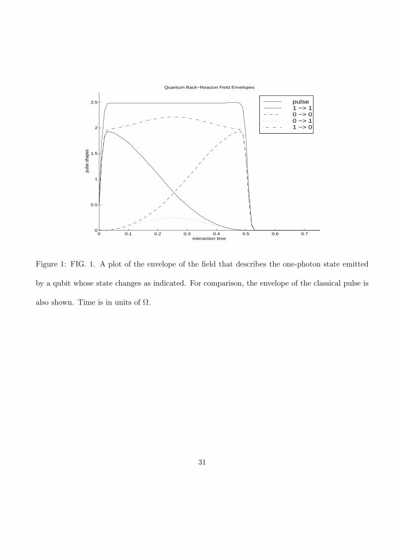
Because all the g functions have significant Fourier components near ω and decay as x−1 like the
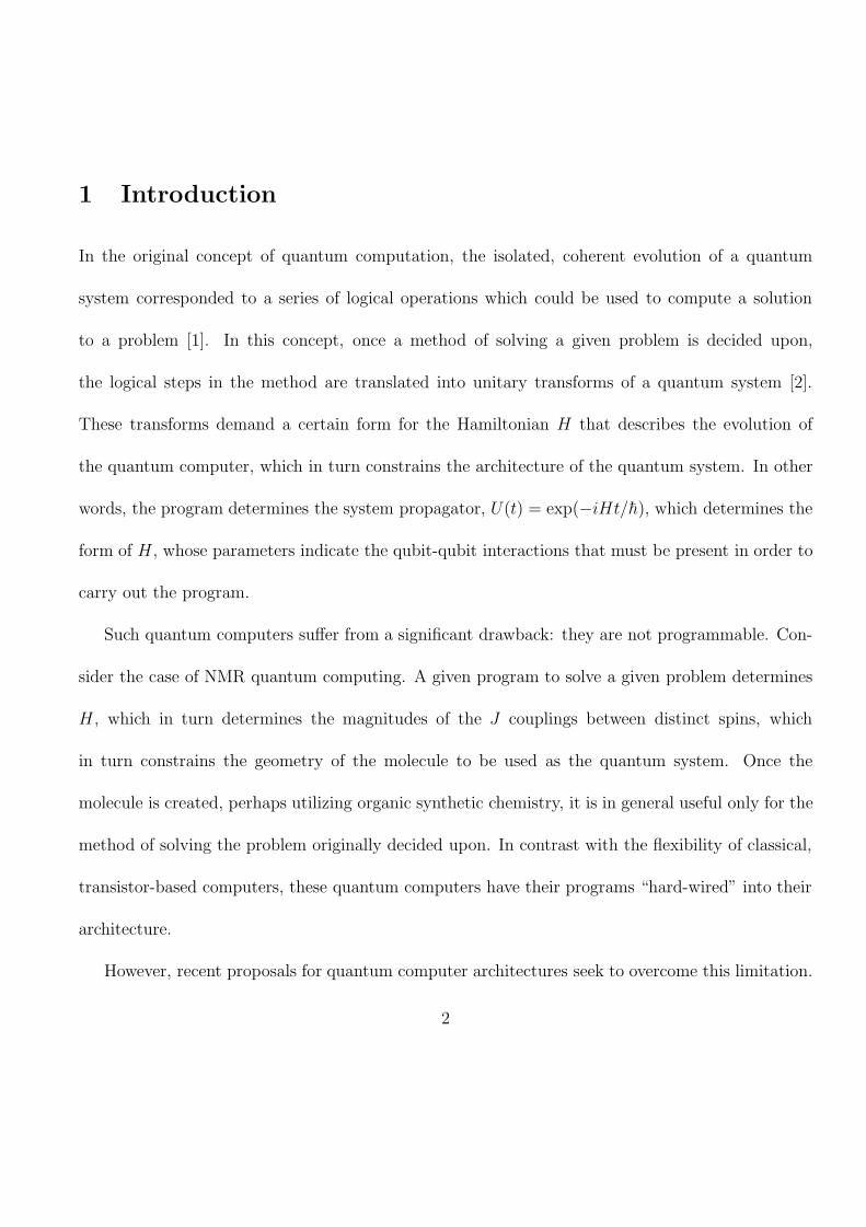
square pulse, the resonator also allows the one-photon states created by the qubit to escape. The
time-domain envelopes of these one-photon states (the Fourier transform of the g functions) are
shown in Fig. 1.
As in the classical field case, the extra phase factors of ±iπ/√8 in the transformation Eq. (14)
15
can be dropped, since they can be compensated for by proper timing. Similarly, we assume φ = 0
at the start of the interaction. The φ term does indicate a curious feature of the back reaction: g−
contains no term from the classical field, while g+ requires two interactions with the classical field
in order to perturb the coherent state. This is consistent with the property that the removal of a
photon from a coherent state does not alter it, while the addition of a photon does.
We can rewrite the transform Eq. (14) in terms of unitary field operators,
i√2
1 1
1 −1
+κ
4Ω
√hωn
2 ε0L3
√Iβ Gβ
√I− G−
√I+ G+
√Iα Gα
(15)
where the G operators create normalized one-photon field states, so that G†G = 1. The normaliza-
tion factors were found by numerical integration, for which the slowly varying√ω term was ignored:
Iα =∫∞−∞ |gα(x)|2dx = 4.297, Iβ = 4.297, I+ = 0.617, and I− = 10.451. Although the G|vac〉 states
are orthogonal to the initial coherent state, they are not mutually orthogonal. Later on, we will
require their (non-normalized) overlap integrals Iα,β =√IαIβ〈vac|G†αGβ|vac〉 =
∫∞−∞ g
?α(x)gβ(x)dx
= 0.614 + i2.221, Iα,+ = −0.617 + i1.110, Iα,− = 4.300 − i3.331, Iβ,+ = 0.617 + i1.110, Iβ,− =
−4.300− i3.331, and I+,− = −1.850.
The important result of this section is the transformation, Eq. (15). Each qubit / field inter-
action has a probability amplitude, proportional to Ω−1, to entangle the qubit with a field state
orthogonal to the original field state. The greater Ω, the lesser the decoherence via this mecha-
nism. Actually, this may seem counterintuitive. Consider the interference pattern produced by a
16
coherent beam of electrons incident upon a double slit. Now allow a laser to interact with one of
the two paths the electron could travel from the slit to the detector. If photons are scattered out of
the coherent modes into vacuum states, then the visibility of the interference pattern is degraded,
as expected [10]. If, however, only stimulated processes are important, then the visibility of the
interference pattern should increase as the laser intensity is increased. The Poisson statistics of a
coherent state can more efficiently hide the information about which path the electron takes as the
number of photons in the beam increases. A similar situation has been noted with regard to welcher
Weg experiments in atomic interferometry (see e.g. [22]).
3.3 Grover’s Algorithm with a Quantum Walsh-Hadamard Transform
Taking the result from the previous section, Grover’s algorithm is now
steps∏j
[ K∏n=1
1− iκ
8Ω
√hωn
ε0L3A(n, tj+1)
WRWK∏
n=1
1− iκ
8Ω
√hωn
ε0L3B(n, tj)
O ] (1√2K
∑x
|x〉)|vac〉
(16)
The displacement operators are not shown. They have been commuted all the way left, picking up
the appropriate phase factors representing the propagation of the free field. The A and B are from
transform Eq. (15), from which a factor of W(n) is first removed:
A =
√IβGβ +
√I−G−
√IβGβ −
√I−G−
√I+G+ +
√IαGα
√I+G+ −
√IαGα
B =
√IβGβ +
√I+G+
√I−G− +
√IαGα√
IβGβ −√I+G+
√I−G− −
√IαGα
(17)
17
The fact that operators acting independently upon separate qubits and field modes mutually com-
mute was also used.
When Eq. (16) is expanded out and only the lowest order terms are kept, to the original
Grover’s transform are added new terms. As previously discussed, the field operators in front of
each term, one for each qubit and each pulse, create field states that are both mutually orthogonal,
and orthogonal to the original field state. Thus, the probability that the final qubit state is |y〉 is the
sum of the probabilities for each of separate terms to be in |y〉. In order to preserve normalization
to O(Ω−2), the total probability to be in an orthogonal field state is subtracted from the probability
of finding the field still in the original state at the end of the algorithm. The goal of this section is
to calculate the success of this implementation of Grover’s algorithm.
After j successful steps of the algorithm, the computer state is given by
cos(jϕ)√2K − 1
∑x 6=y
|x〉+ sin(jϕ) |y〉 |vac〉
where sinϕ = 2√
2K − 1/2K [18]. The general trend for the influence of the back reaction can be
discerned from the specific example of 3 qubits and y = 2. A back reaction on the field can occur
during either application of W. If it occurs immediately after O has been called (the operator B),
or after the invert about average transform (the operator A). Suppose the reaction occurs after O,
and it is for the least significant qubit. Then the computer state becomes
cos(jϕ)√2K − 1
((Bβ |0〉+ B+|1〉) + (Bα|1〉+ B−|0〉) + (Bα|3〉+ B−|2〉) + (Bβ|4〉+ B+|5〉)+
18
(Bα|5〉+ B−|4〉) + (Bβ |6〉+ B+|7〉) + (Bα|7〉+ B−|6〉))− sin(jϕ)
(Bβ |2〉+ B+|3〉
)|vac〉 (18)
The amplitudes of pairs of states that differ at their least significant digit such as (0,1), (2,3), and
so on, are mixed. If the error occurs for the second least significant qubit, then
cos(jϕ)√2K − 1
((Bβ |0〉+ B+|2〉) + (Bα|1〉+ B−|3〉) + (Bα|3〉+ B−|1〉) + (Bβ|4〉+ B+|6〉)+
(Bα|5〉+ B−|7〉) + (Bβ|6〉+ B+|4〉) + (Bα|7〉+ B−|5〉))− sin(jϕ)
(Bβ |2〉+ B+|0〉
)|vac〉 (19)
The difference is in which pairs of states are mixed, and whether the qubit involved in the back
reaction was initially in state 0 or 1. Using this, we can sum over all the qubits of the computer,
the total probability for a back reaction to occur during the first of the two applications of W, at
step j in the algorithm. Suppose that the qubit frequencies are sufficiently close so that all pulse
center frequencies are ω. Then
(κ
8Ω
)2 hω
ε0
[K
2
2K − 2
2K − 1cos2(jϕ)
(|(Bβ + B−)|vac〉|2 + |(Bα + B+)|vac〉|2
)+
(K − ‖y‖)( ∣∣∣∣∣ cos(jϕ)√
2K − 1B−|vac〉 − sin(jϕ)Bβ|vac〉
∣∣∣∣∣2
+
∣∣∣∣∣ cos(jϕ)√2K − 1
Bα|vac〉 − sin(jϕ)B+|vac〉∣∣∣∣∣2 )
+
‖y‖( ∣∣∣∣∣ cos(jϕ)√
2K − 1Bβ|vac〉 − sin(jϕ)B−|vac〉
∣∣∣∣∣2
+
∣∣∣∣∣ cos(jψ)√2K − 1
B+|vac〉 − sin(jϕ)Bα|vac〉∣∣∣∣∣2 )]
The factor ‖y‖ appears since the back reaction depends upon whether a qubit was initially in state
0 or 1. Now suppose K is large enough so that 2K 1. The following approximations are useful:
∑π/2ϕj=1 cos2(jϕ) ≈ ∫ π/2
0 cos2 x dx/ϕ = π/4ϕ, and∑π/2ϕ
j=1 sin2(jϕ) ≈ π/4ϕ, and∑π/2ϕ
j=1 sin(jϕ) cos(jϕ)
19
≈ 1/2ϕ. Again, keeping only the largest terms in K, the probability that a back reaction occurs
for any qubit, and at any step, during the first of the two W transforms is given by
(κ
8Ω
)2 hω
ε0
π
82K/2
[K
2
(|(Bβ + B+)|vac〉|2 + |(Bα + B+)|vac〉|2
)
+(K − ‖y‖)(|Bβ|vac〉|2 + |B+|vac〉|2
)+ ‖y‖
(|B−|vac〉|2 + |Bα|vac〉|2
)](20)
If the back reaction occurs during the second W in an iteration, then j starts at 2 (the first invert-
about-average step is always carried out), and the sign of the amplitude for |y〉 is positive. Taking
the limit for large K, the cross-terms that depend upon the sign of ay drop out, and the final
expression is the same as above except with the B operators replaced by those of A. The total
probability of a back reaction anywhere in the algorithm is then the sum of these two. Starting
with the operators of Eq. (17), the matrix elements are expressed in terms of the normalization
and overlap of the G|vac〉 states, e.g. |(Bβ +B−)|vac〉|2 + |(Bα +B+)|vac〉|2 = 2(Iα + Iβ + I+ + I−)
+ 4<e(Iβ,− + Iα,+). Plugging in, the final probability to end up entangled with an orthogonal field
state is (κ
Ω
)2 hω
ε0
√2K
(0.211K + 0.241‖y‖
). (21)
How much do the orthogonal field states contribute to the correct final answer? First, note that
the matrix elements of A and B all have similar magnitudes. Thus, they equally mix the state |y〉
with the state connected to it by flipping the qubit that experiences the back reaction. Early in
the algorithm when sin(jϕ) 1, this does not increase the amplitude in ay significantly, since the
20
state that mixes with |y〉 has amplitude cos(jϕ)/√
2K 1. At later times, however, the amplitude
of |y〉 is near 1, so the back reaction decreases the probability to be in state |y〉 by roughly half.
Thus, after j iterations of Grover’s algorithm, a back reaction will cause the result to appear
as if only ≈ j/2 iterations had been performed. Further iterations will continue to transform these
entangled states, but this does not necessarily improve the final result. Recall from Eq. (1) that
amplitude is rotated into |y〉 only when the signs of ay and∑
x 6=y |x〉 are the same. For large K, the
amplitude ay is ≈ sin(jϕ) (√IβGβ +
√I−G−)|vac〉. The other qubit states are entangled with field
states that are partly orthogonal to this state, but the amplitude that lies along the same direction in
the Hilbert space of the field is, for largeK, cos(jϕ) (Iβ + Iβ,+ + I−,β + I−,+) /√Iβ + I− + 2<e(Iβ,−)
= (−2.232+ i0.448) cos(jϕ). The real part has switched sign, and so further iterations will actually
remove amplitude from |y〉. It should be clear that the back reaction essentially scrambles the
memory of the quantum computer, from which further iterations will not, in general, recover the
correct amplitude before the computation ends.
4 Quantum Back Reaction for the CNOT Gate
In this section, we briefly examine what happens when a classical field is used to drive a logic gate,
such as R, that entangles together separate qubits. As before, let us focus on a single example,
that of the controlled-NOT (CNOT) gate. CNOT is defined as a transform acting on two qubits
21
that flips the second qubit only if the first qubit is 1: |00〉 → |00〉, |01〉 → |01〉, |10〉 → |11〉, and
|11〉 → |10〉. As for the Walsh-Hadamard transform, there are numerous ways to implement the
CNOT gate [5]. Perhaps the most straight forward method is the use of a selective pulse. What we
mean by this is the following.
The two qubits to be transformed by CNOT have a Hamiltonian
H/h = ω1Sz + ω2Iz + J ~S · ~I +∑~k
ωa~k†a~k + κ
(Sx + Ix
)(E+ + E−
). (22)
By ~S · ~I we mean the qubit operator SxIx+ SyIy+ SzIz. Assume that ω2 > ω1 |ω1 − ω2|
J . In this case, the transitions driven by the field occur at ≈ ω1 ± J/2 + J2/4(ω1 − ω2) and ≈
ω2±J/2−J2/4(ω1−ω2), They appear as a “doublet of doublets”, that is, two sets of two lines each.
Since H is nearly diagonal for small J , the highest frequency transition corresponds to |10〉 ↔ |11〉.
Thus, a CNOT gate can be implemented by selectively inverting this transition with a square pulse
of duration T 2π/J . (T also depends on the matrix element for the transition.) The long length
of the pulse keeps its bandwidth small enough so that it does not significantly overlap with the
other transitions in the system.
As before, first assume that the pulse is described by a coherent field state, and commute the
displacement operator to the left. This replaces E± with E± + Ee∓iωt in Eq. (22). Second, split
H = HC + HQ, where HQ contains the electric (or magnetic) field operators terms. Suppose we
find UC(t), the propagator corresponding to HC . Then the total propagator for the system can be
22
formally integrated as
U(t) = UC(t)− i
h
∫ t
0dt′UC(t−t′)HQUC(t′) − 1
h2
∫ t
0dt′∫ t′
0dt′′ UC(t−t′)HQUC(t′−t′′)HQUC(t′′)+ · · ·
(23)
Computing the value of the first integral in this series is the goal of this section. As before, this
integral can be physically interpreted as follows: the qubit evolves under UC , coherently evolving
under the influence of a classical field until time t′, when a scattering event occurs due to the
quantum nature of the field. After the scattering, the qubit / field system evolves as before until
final time t. Higher order corrections then correspond to multiple scatterings (or, multiple field
operators). To find UC , first assume a solution of the form exp(−i∑ωa~k†a~k) exp(−iω[Sz + Iz]t)
UC1, and then drop the rapidly oscillating terms. Then diagonalize the resulting Hamiltonian,
HC1 =
(ω1+ω2)/2− ω+J/4 κE/2 κE/2 0
κE/2 (ω1−ω2)/2−J/4 J/2 κE/2
κE/2 J/2 (−ω1+ω2)/2−J/4 κE/2
0 κE/2 κE/2 −(ω1+ω2)/2+ω+J/4
,
to find eigenvalues λn and eigenvectors vn. Plugging in the UC operator into Eq. (23), and as before
keeping only the terms linear in the creation operators, the lowest order quantum back reaction is
(in the rotating frame)
−κ2
∑~k
ei~k·~r√
hω
2ε0L3a~k
†4∑
n,m=1
vnv†n(S− + I−)v†mvme
iλnT ei(ω−ω+λm−λn)t − 1
i(ω − ω + λm − λn)
23
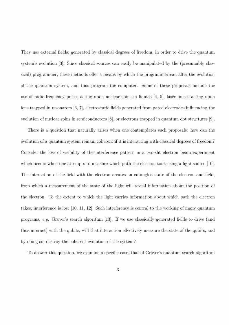
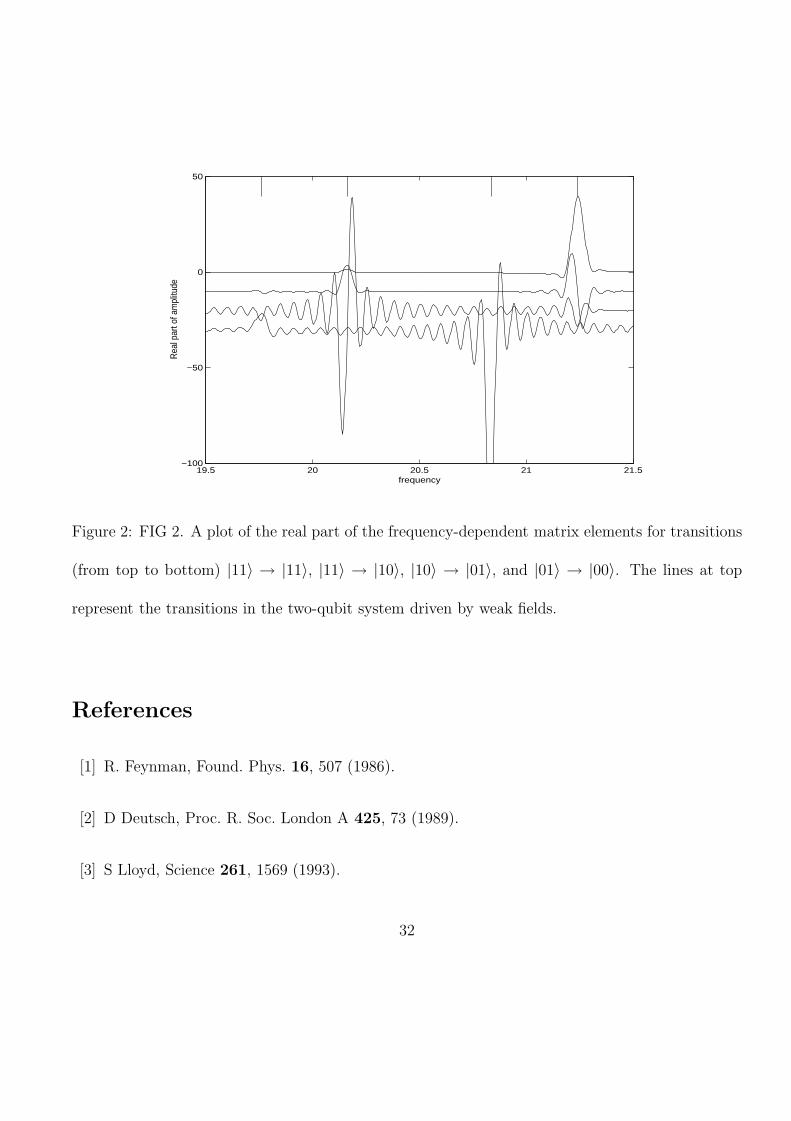
The real parts of the field amplitudes of the one-photon states entangled with different qubit states
for a few of the matrix elements of U are shown in Fig. 2. The parameters used to generate the
figure were ω1 = 20, ω2 = 21, and J = 0.4 for the qubits, and κE = 0.01, and T = 100.6 for the
classical pulse profile. The classical result, UC(T ), transfers 97% of the amplitude between states
|11〉 and |10〉. These parameters are not meant to represent any specific spectroscopic method.
For on-resonant transitions, the matrix element peaks strongly at T ∝ E−1. Thus, as before,
weaker pulses lead to greater decoherence. The matrix element for the transition |01〉 → |00〉 is
found to have the greatest magnitude. It may be surprising that transitions that are not being
driven by the external field can also have large decoherence rates. Recall that this method of
implementing the CNOT gate actually drives all the allowed transitions, but is only resonant with
one of them. This decoherence process continues to grow because these other transitions that can
lead to photon emission are weakly but continuously excited.
In summary, several conclusions are of interest. First, the field states that become entangled with
the two-qubit states are orthogonal to the initial field state, but they are not mutually orthogonal.
In fact, their projections onto one another have essentially random phases. Computations that
use the phases of the qubit state will be scrambled by this process. Secondly, because the CNOT
gate involves entangling separate qubits, the scattering process also involves creating mutually
entangled qubit / field states. It appears reasonable to suggest that this kind of field / multiple
qubit entanglement will result when such logic gates are driven by external fields.
24
5 Discussion
5.1 Grover’s algorithm
When unitary transforms are driven by externally generated coherent fields in the manner dis-
cussed above, a decoherence mechanism exists that, with each applied pulse, tends to scramble the
computer’s memory. This decoherence mechanism is slightly different from the usual environmen-
tally induced decoherence, in that it increases as the number of times the programmer attempts
to manipulate the qubit system coherently. In the case of Grover’s search algorithm where the
Walsh-Hadamard transforms are externally driven, the degradation of the correct response scales
as 0.2K2K/2(hω/ε0L3)(κ/Ω)2
A criticism of this analysis might be in the specific choice used to implement W(n). Whatever
method is chosen, the field / qubit propagators still hold, and some back reaction must exist (but
see below). In general, the degradation should scale as the number of times a qubit transform is
driven. For Grover’s algorithm, if no error correction routines are implemented, then the amplitude
Ω of the field will have to increase exponentially with increasing K in order to keep the error below
a fixed bound. Clearly, this is not a scalable way to implement Grover’s algorithm.
How important is this decoherence mechanism to the different proposed quantum computer
schemes? Let us employ simple order of magnitude arguments, and ignore for the moment the
implementation of error-correcting codes. The total probability for decoherence can also be written
25
as 0.2 [(hω)/(L3ε0E2/2)] K2K/2. The pre-factor is the ratio of the energy of a single photon, to
the total energy in the pulse (energy density times resonator volume), or the reciprocal of the total
number of photons in the resonator used to create a pulse.
First, examine the case for using lasers to drive single ions or atoms. A recent experimental
demonstration of a logic gate using trapped 9Be+ ions as qubits [23] used 1 mW pulses of ≈ 10−4
s duration at 300 nm. This corresponds to 1012 photons per pulse. The very small pre-factor will
not pose a problem for computations involving a polynomial number of steps with increasing K,
but for Grover’s algorithm this mechanism limits the number of qubits to ≈ 70.
Next, suppose we examine the case for NMR quantum computing. First, let us address the
question of utilizing the signal from a large number of independent quantum computers. Let us
assume that our sample can be prepared in the ground state (all spins initially down), and let us
ignore the interaction of the computers with one another through the field. We note that these
assumptions are hardly justified for real world systems, but assuming a finite temperature for
bulk quantum computing causes separate difficulties that have been addressed elsewhere [24]. The
application of Grover’s algorithm results in a final state
|Ψ〉 =1023∏i = 1
((1− γ2/2)|y(i)〉+ γ
∑x
G(x)|x(i)〉)|vac〉
where G creates orthogonal field states that contribute little amplitude to the correct solution. The
total signal is the sum from all of the quantum computers in the sample, 〈Ψ|∑i
(|y(i)〉〈y(i)|
)|Ψ〉 = N
(1−γ2/2). The point is that at low temperatures, the macroscopic decoherence rate is multiplied by
26
the total number of independent quantum computers in the sample. Typically, NMR uses ν ≈ 108
Hz, or a photon energy of 10−25 J. Pulses are 100 W for 10 µs, for a total energy of 10−3 J. Thus,
there are 1022 photons per pulse. This limits Grover’s algorithm for NMR to ≈ 140 qubits if we can
do NMR on a single spin system; but for a micro-mole (1017) of quantum computers, we are limited
to roughly 25 qubits. If electron spin resonance is substituted as the spectroscopic technique, then
ν ≈ 1010 Hz, pulses are 1 kW for 10 ns, and thus require 1018 photons, a negligible improvement
over NMR.
If, as is usually the case, Ω ωn, then the number of photons required to generate W(n) is
proportional to Ω/(κ2ωn). Thus, physical systems with small values of ωn or κ are the most resistant
to the above decoherence mechanism. Unfortunately, such systems have other limitations: if ωn is
small, then the temperature of the system is required to scale with increasing K in an unfortunate
manner [24], while κ is small, then the time required to drive the qubits increases, which in turn
slows the entire computation down. It seems that quantum computers driven or programmed by
externally applied fields will face significant design trade-offs.
Will driving qubits by externally applied, static electric fields [8] offer any significant advantages?
(Similar proposals might be envisioned for NMR by applying different static magnetic fields along
different directions to individual spins.) In the Coulomb gauge, such longitudinal fields are not
independent degrees of freedom [25]. Instead, the total Hamiltonian of such a system must include
the particles whose charges give rise to the static fields. Thus, for the case of qubits driven by
27
electrostatic fields from electrodes, decoherence results from the field operators (now with half
integer spin statistics) for the Fermi levels of each electrode becoming entangled with the qubit
operators. Finding the decoherence rate in this case is complicated by the extra structure for
the electrons in the electrode, but it would be surprising if some decoherence mechanism was not
present.
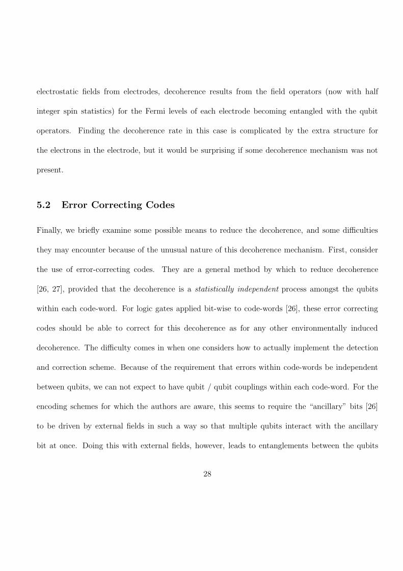
5.2 Error Correcting Codes
Finally, we briefly examine some possible means to reduce the decoherence, and some difficulties
they may encounter because of the unusual nature of this decoherence mechanism. First, consider
the use of error-correcting codes. They are a general method by which to reduce decoherence
[26, 27], provided that the decoherence is a statistically independent process amongst the qubits
within each code-word. For logic gates applied bit-wise to code-words [26], these error correcting
codes should be able to correct for this decoherence as for any other environmentally induced
decoherence. The difficulty comes in when one considers how to actually implement the detection
and correction scheme. Because of the requirement that errors within code-words be independent
between qubits, we can not expect to have qubit / qubit couplings within each code-word. For the
encoding schemes for which the authors are aware, this seems to require the “ancillary” bits [26]
to be driven by external fields in such a way so that multiple qubits interact with the ancillary
bit at once. Doing this with external fields, however, leads to entanglements between the qubits
28
within the code-word and the external fields. This in turn means that errors developed during the
error correction scheme itself will not have the required statistical independence. However, in order
to better understand how this decoherence mechanism might influence error correcting schemes, it
would be helpful to examine a complete program, such as Grover’s algorithm with a specific code
implemented.
Perhaps more hopefully, it appears that there are independent means by which storing infor-
mation in multiple qubits could reduce this decoherence mechanism. Note that the appearance of
terms such as |Bβ +B−| in Eq. (20) shows that destructive interference can lessen the probability of
a back reaction. It is known to be possible to quench spontaneous emission in multi-level systems
[28], which is a process quite similar to the decoherence mechanism considered here. Thus, it seems
likely that a similar design could be used to remove the lowest order terms in the expansion of Eq.
(23). Then, the decoherence rate increases as the inverse square of the number of photons in a
pulse, which can be considered as a significant improvement.
Conclusions
Quantum computers that use external, classically generated electromagnetic fields to drive the
evolution of the system undergo a decoherence induced by the quantum back reaction to those
fields. The probability for the quantum system to be degraded increases as the total number of
externally driven transforms, and inversely as the number of photons in the pulse. For algorithms in
which no error-correcting codes are implemented, and for which the number of pulses is required to
29
increase exponentially as the problem size increases, the field intensity driving the system will also
be required to increase exponentially in order to bound the degradation of the response. And for the
implementation of error-correcting codes, the use of external fields for error detection and correction
gives rise to a decoherence that does not have the property of being statistically independent between
separate qubits in the code-word.
Acknowledgements
We gratefully acknowledge support from the Air Force Office of Scientific Research.
30
0 0.1 0.2 0.3 0.4 0.5 0.6 0.70
0.5
1
1.5
2
2.5
interaction time
pulse
sha
pes
Quantum Back−Reacion Field Envelopes
pulse1 −> 10 −> 00 −> 11 −> 0
Figure 1: FIG. 1. A plot of the envelope of the field that describes the one-photon state emitted
by a qubit whose state changes as indicated. For comparison, the envelope of the classical pulse is
also shown. Time is in units of Ω.
31
19.5 20 20.5 21 21.5−100
−50
0
50
frequency
Rea
l par
t of a
mpl
itude
Figure 2: FIG 2. A plot of the real part of the frequency-dependent matrix elements for transitions
(from top to bottom) |11〉 → |11〉, |11〉 → |10〉, |10〉 → |01〉, and |01〉 → |00〉. The lines at top
represent the transitions in the two-qubit system driven by weak fields.
References
[1] R. Feynman, Found. Phys. 16, 507 (1986).
[2] D Deutsch, Proc. R. Soc. London A 425, 73 (1989).
[3] S Lloyd, Science 261, 1569 (1993).
32
[4] J. A. Jones, M. Mosca, J. Chem. Phys. 109, 1648 (1998).
[5] D. G. Cory, A. F. Fahmy, and T. F. Havel, in Proceedings of the Fourth Workshop on Physics
and Computation, edited by T. Toffoli (New England Complex Systems Institute, Boston,
1996), pp.87-91.
[6] J. I. Cirac, P. Zoller, Phys. Rev. Lett. 74, 4091 (1995).
[7] S. Schneider, D. F. V. James, and G. J. Milburn, e-print quant-ph/9808012.
[8] B. E. Kane, Nature 393, 133 (1998).
[9] D. S. Chemla, D. A. B. Miller, in Heterojunction Band Discontinuities, Physics, and Device
Applications., edited by F. Capasso and G. Margaritondo (North-Holland, Elsevier, New York,
1987).
[10] R. Feynman, Leighton, Sands, The Feynman Lectures on Physics, Volume III (Addison-Wesley,
Reading, MA, 1965). Ch. 3.
[11] D. Giulini et al., Decoherence and the Appearance of a Classical World in Quantum Theory
(Springer, Berlin, 1996).
[12] W. Zurek, Phys. Today 44, 36 (1991).
[13] L. Grover, Phys. Rev. Lett. 79, 325 (1997).
33
[14] N. Imoto, Prog. Crystal Growth and Charact. 33, 295 (1996).
[15] M. R. Garey and D. S. Johnson, Computers and Intractability. A Guide to the Theory of NP
Completeness. (W. H. Freeman, New York, 1979).
[16] C. H. Bennet, E. Bernstein, G. Brassard, and U. Vazirani, e-print quant-ph/9701001.
[17] M. Boyer et al., e-print quant-ph/9605034.
[18] C. Zalka, e-print quant-ph/9711070.
[19] R. R. Ernst, G. Bodenhausen, and A. Wokaun, Principals of Nuclear Magnetic Resonance in
One and Two Dimensions. (Clarendon Press, Oxford, 1987).
[20] The assumption κE J is useful to implement single qubit interactions only. In NMR termi-
nology, it corresponds to the transformation of magnetization from a given spin, irregardless
of J-J couplings (or hyperfine couplings for the case of ESR). Implementing transforms that
entangle separate qubits, however, can involve the use of selective pulses that manipulate the
magnetization within the J-J coupling (or hyperfine couplings) manifold, as shown for the
CNOT gate.
[21] L. Mandel and E. Wolf, Optical Coherence and Quantum Optics. (Cambridge University Press,
Cambridge, 1995). Ch. 11.13.
[22] M. O. Scully, B.-G. Englert, and H. Walther, Nature 351, 111 (1991).
34
[23] C. Monroe et al., Phys. Rev. Lett. 75, 4714 (1995).
[24] W. S. Warren, Science 277, 1688 (1997).
[25] C. Cohen-Tannoudji, J. Dupont-Roc, and G. Grynberg, Photons & Atoms: Introduction to
Quantum Electrodynamics. (Wiley, New York, 1989).
[26] P. Shor, in Proceedings, 35th Annual Symposium on Foundations of Computer Science. (IEEE
Press, New York, 1994), pp.56-65.
[27] E. Knill and R. Laflamme, Phys. Rev. A 55, 900 (1997).
[28] H. Lee, P. Polynkin, M. O. Scully, and S.-Y. Zhu, Phys. Rev. A 55, 4454 (1997).
35