Decoding, Calibration and Rectification for Lenselet-Based Plenoptic Cameras

Donald G. Dansereau, Oscar Pizarro and Stefan B. WilliamsAustralian Centre for Field Robotics; School of Aerospace, Mechanical and Mechatronic Engineering

University of Sydney, NSW, Australia{d.dansereau, o.pizarro, s.williams}@acfr.usyd.edu.au

Abstract

Plenoptic cameras are gaining attention for their uniquelight gathering and post-capture processing capabilities.We describe a decoding, calibration and rectification pro-cedure for lenselet-based plenoptic cameras appropriate fora range of computer vision applications. We derive a novelphysically based 4D intrinsic matrix relating each recordedpixel to its corresponding ray in 3D space. We furtherpropose a radial distortion model and a practical objec-tive function based on ray reprojection. Our 15-parametercamera model is of much lower dimensionality than cam-era array models, and more closely represents the physicsof lenselet-based cameras. Results include calibration of acommercially available camera using three calibration gridsizes over five datasets. Typical RMS ray reprojection er-rors are 0.0628, 0.105 and 0.363 mm for 3.61, 7.22 and35.1 mm calibration grids, respectively. Rectification ex-amples include calibration targets and real-world imagery.

1. Introduction

Plenoptic cameras [17] measure both colour and geo-

metric information, and can operate under conditions pro-

hibitive to other RGB-D cameras, e.g. in bright sunlight or

underwater. With increased depth of field and light gather-

ing relative to conventional cameras, and post-capture ca-

pabilities ranging from refocus to occlusion removal and

closed-form visual odometry [1, 16, 4, 9, 19, 6], plenop-

tic cameras are poised to play a significant role in computer

vision applications. As such, accurate plenoptic calibration

and rectification will become increasingly important.

Prior work in this area has largely dealt with camera ar-

rays [20, 18], with very little work going toward the cali-

bration of lenselet-based cameras. By exploiting the phys-

ical characteristics of a lenselet-based plenoptic camera,

we impose significant constraints beyond those present in

a multiple-camera scenario. In so doing, we increase the

robustness and accuracy of the calibration process, while

simultaneously decreasing the complexity of the model.

In this work we present a novel 15-parameter plenop-

tic camera model relating pixels to rays in 3D space, in-

cluding a 4D intrinsic matrix based on a projective pinhole

and thin-lens model, and a radial direction-dependent dis-

tortion model. We present a practical method for decod-

ing a camera’s 2D lenselet images into 4D light fields with-

out prior knowledge of its physical parameters, and describe

an efficient projected-ray objective function and calibration

scheme. We use these to accurately calibrate and rectify im-

ages from a commercially available Lytro plenoptic camera.

The remainder of this paper is organized as follows: Sec-

tion 2 reviews relevant work; Section 3 provides a practical

method for decoding images; Section 4 derives the 4D in-

trinsic and distortion models; Section 5 describes the cali-

bration and rectification procedures; Section 6 provides val-

idation results; and finally, Section 7 draws conclusions and

indicates directions for future work.

2. Prior WorkPlenoptic cameras come in several varieties, including

mask-based cameras, planar arrays, freeform collections of

cameras [13, 22, 21, 18], and of course lenticular array-

based cameras. The latter include the “original” plenop-

tic camera as described by Ng et al. [17], with which the

present work is concerned, and the “focused” plenoptic

camera described by Lumsdaine and Georgiev [14]. Each

camera has unique characteristics, and so the optimal model

and calibration approach for each will differ.

Previous work has addressed calibration of grids or

freeform collections of multiple cameras [20, 18]. Similar

to this is the case of a moving camera in a static scene, for

which structure-from-motion can be extended for plenoptic

modelling [12]. These approaches introduce more degrees

of freedom in their models than are necessary to describe

the lenselet-based plenoptic camera. Our work introduces

a more constrained intrinsic model based on the physical

properties of the camera, yielding a more robust, physically-

grounded, and general calibration.

2013 IEEE Conference on Computer Vision and Pattern Recognition

1063-6919/13 $26.00 © 2013 IEEE

DOI 10.1109/CVPR.2013.137

1025

2013 IEEE Conference on Computer Vision and Pattern Recognition

1063-6919/13 $26.00 © 2013 IEEE

DOI 10.1109/CVPR.2013.137

1025

2013 IEEE Conference on Computer Vision and Pattern Recognition

1063-6919/13 $26.00 © 2013 IEEE

DOI 10.1109/CVPR.2013.137

1025

2013 IEEE Conference on Computer Vision and Pattern Recognition

1063-6919/13 $26.00 © 2013 IEEE

DOI 10.1109/CVPR.2013.137

1027

2013 IEEE Conference on Computer Vision and Pattern Recognition

1063-6919/13 $26.00 © 2013 IEEE

DOI 10.1109/CVPR.2013.137

1027

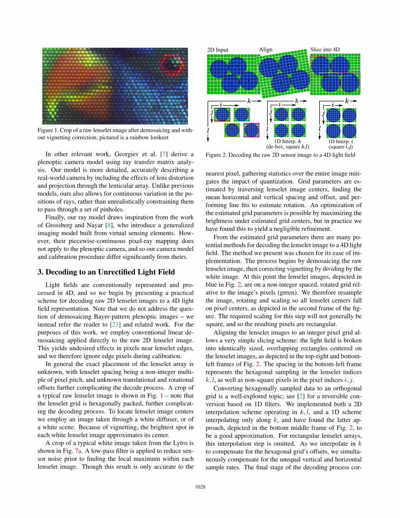
Figure 1. Crop of a raw lenselet image after demosaicing and with-

out vignetting correction; pictured is a rainbow lorikeet

In other relevant work, Georgiev et al. [7] derive a

plenoptic camera model using ray transfer matrix analy-

sis. Our model is more detailed, accurately describing a

real-world camera by including the effects of lens distortion

and projection through the lenticular array. Unlike previous

models, ours also allows for continuous variation in the po-

sitions of rays, rather than unrealistically constraining them

to pass through a set of pinholes.

Finally, our ray model draws inspiration from the work

of Grossberg and Nayar [8], who introduce a generalized

imaging model built from virtual sensing elements. How-

ever, their piecewise-continuous pixel-ray mapping does

not apply to the plenoptic camera, and so our camera model

and calibration procedure differ significantly from theirs.

3. Decoding to an Unrectified Light FieldLight fields are conventionally represented and pro-

cessed in 4D, and so we begin by presenting a practical

scheme for decoding raw 2D lenselet images to a 4D light

field representation. Note that we do not address the ques-

tion of demosaicing Bayer-pattern plenoptic images – we

instead refer the reader to [23] and related work. For the

purposes of this work, we employ conventional linear de-

mosaicing applied directly to the raw 2D lenselet image.

This yields undesired effects in pixels near lenselet edges,

and we therefore ignore edge pixels during calibration.

In general the exact placement of the lenselet array is

unknown, with lenselet spacing being a non-integer multi-

ple of pixel pitch, and unknown translational and rotational

offsets further complicating the decode process. A crop of

a typical raw lenselet image is shown in Fig. 1 – note that

the lenselet grid is hexagonally packed, further complicat-

ing the decoding process. To locate lenselet image centers

we employ an image taken through a white diffuser, or of

a white scene. Because of vignetting, the brightest spot in

each white lenselet image approximates its center.

A crop of a typical white image taken from the Lytro is

shown in Fig. 7a. A low-pass filter is applied to reduce sen-

sor noise prior to finding the local maximum within each

lenselet image. Though this result is only accurate to the

�����������

������������������������������

����������������������

�

�

��

�

�

�� �

�

��

������������

Figure 2. Decoding the raw 2D sensor image to a 4D light field

nearest pixel, gathering statistics over the entire image miti-

gates the impact of quantization. Grid parameters are es-

timated by traversing lenselet image centers, finding the

mean horizontal and vertical spacing and offset, and per-

forming line fits to estimate rotation. An optimization of

the estimated grid parameters is possible by maximizing the

brightness under estimated grid centers, but in practice we

have found this to yield a negligible refinement.

From the estimated grid parameters there are many po-

tential methods for decoding the lenselet image to a 4D light

field. The method we present was chosen for its ease of im-

plementation. The process begins by demosaicing the raw

lenselet image, then correcting vignetting by dividing by the

white image. At this point the lenselet images, depicted in

blue in Fig. 2, are on a non-integer spaced, rotated grid rel-

ative to the image’s pixels (green). We therefore resample

the image, rotating and scaling so all lenselet centers fall

on pixel centers, as depicted in the second frame of the fig-

ure. The required scaling for this step will not generally be

square, and so the resulting pixels are rectangular.

Aligning the lenselet images to an integer pixel grid al-

lows a very simple slicing scheme: the light field is broken

into identically sized, overlapping rectangles centered on

the lenselet images, as depicted in the top-right and bottom-

left frames of Fig. 2. The spacing in the bottom-left frame

represents the hexagonal sampling in the lenselet indices

k, l, as well as non-square pixels in the pixel indices i, j.

Converting hexagonally sampled data to an orthogonal

grid is a well-explored topic; see [2] for a reversible con-

version based on 1D filters. We implemented both a 2D

interpolation scheme operating in k, l, and a 1D scheme

interpolating only along k, and have found the latter ap-

proach, depicted in the bottom middle frame of Fig. 2, to

be a good approximation. For rectangular lenselet arrays,

this interpolation step is omitted. As we interpolate in kto compensate for the hexagonal grid’s offsets, we simulta-

neously compensate for the unequal vertical and horizontal

sample rates. The final stage of the decoding process cor-

10261026102610281028

��

��

��� ���

�

�� ��Figure 3. The main lens is modelled as a thin lens and the lenselets

as an array of pinholes; gray lines depict lenselet image centers

rects for the rectangular pixels in i, j through a 1D interpo-

lation along i. In every interpolation step we increase the

effective sample rate in order to avoid loss of information.

The final step, not shown, is to mask off pixels that fall out-

side the hexagonal lenselet image. We denote the result of

the decode process the “aligned” light field LA(i, j, k, l).

4. Pinhole and Thin Lens ModelIn this section we derive the relationship between the

indices of each pixel and its corresponding spatial ray.

Though each pixel of a plenoptic camera integrates light

from a volume, we approximate each as integrating along a

single ray [8]. We model the main lens as a thin lens, and

the lenselets as an array of pinholes, as depicted in Fig. 3.

Our starting point is an index resulting from the decoding

scheme described above, expressed in homogeneous coor-

dinates n = [i, j, k, l, 1], where k, l are the zero-based ab-

solute indices of the lenselet through which a ray passes,

and i, j are the zero-based relative pixel indices within each

lenselet image. For lenselet images of N ×N pixels, i and

j each range from 0 to N − 1.

We derive a homogeneous intrinsic matrix H ∈ R5×5

by applying a series of transformations, first converting the

index n to a ray representation suitable for ray transfer ma-

trix analysis, then propagating it through the optical system,

and finally converting to a light field ray representation. The

full sequence of transformations is given by

φA = HφΦH

MHTHΦφH

φabsH

absreln = Hn. (1)

We will derive each component of this process in the 2D

plane, starting with the homogenous relative index n2D =[i, k, 1], and later generalize the result to 4D.

The conversion from relative to absolute indices, Habsrel

is straightforwardly found from the number of pixels per

lenselet N and a translational pixel offset cpix (below). We

next convert from absolute coordinates to a light field ray,

with the imaging and lenselet planes as the reference planes.

We accomplish this using Hφabs,

Habsrel =

[1 N -cpix0 1 00 0 1

], Hφ

abs =

[1/Fs 0 -cM/Fs

0 1/Fu -cμ/Fu

0 0 1

], (2)

where F∗ and c∗ are the spatial frequencies in samples/m,

and offsets in samples, of the pixels and lenselets.

Next we express the ray as position and direction via HΦφ

(below), and propagate to the main lens using HT :

HΦφ =

[ 1 0 0-1/dμ 1/dμ 0

0 0 1

], HT =

[1 dμ+dM 00 1 00 0 1

], (3)

where d∗ are the lens separations as depicted in Fig. 3. Note

that in the conventional plenoptic camera, dμ = fμ, the

lenselet focal length.

Next we apply the main lens using a thin lens and small

angle approximation (below), and convert back to a light

field ray representation, with the main lens as the s, t plane,

and the u, v plane at an arbitrary plane separation D:

HM =[

1 0 0-1/fM 1 0

0 0 1

], Hφ

Φ =[1 D 00 1 00 0 1

], (4)

where fM is the focal length of the main lens. Because hor-

izontal and vertical components are independent, extension

to 4D is straightforward. Multiplying through Eq. 1 yields

an expression for H with twelve non-zero terms:[stuv1

]=

⎡⎣H1,1 0 H1,3 0 H1,5

0 H2,2 0 H2,4 H2,5

H3,1 0 H3,3 0 H3,5

0 H4,2 0 H4,4 H4,5

0 0 0 0 1

⎤⎦[

ijkl1

]. (5)

In a model with pixel or lenselet skew we would expect

more non-zero terms. In Section 5 we show that two of

these parameters are redundant with camera pose, leaving

only 10 free intrinsic parameters.

4.1. Projection Through the Lenselets

We have hidden some complexity in deriving the 4D in-

trinsic matrix by assuming prior knowledge of the lenselet

associated with each pixel. As depicted by the gray lines

in Fig. 3, the projected image centers will deviate from the

lenselet centers, and as a result a pixel will not necessarily

associate with its nearest lenselet. Furthermore, the decod-

ing process presented in Section 3 includes several manipu-

lations which will change the effective camera parameters.

By resizing, rotating, interpolating, and centering on the

projected lenselet images, we have created a virtual light

field camera with its own parameters. In this section we

compensate for these effects through the application of cor-

rection coefficients to the physical camera parameters.

Lenselet-based plenoptic cameras are constructed with

careful attention to the coplanarity of the lenselet array and

image plane [17]. As a consequence, projection through

the lenselets is well-approximated by a single scaling fac-

tor, Mproj . Scaling and adjusting for hexagonal sampling

can similarly be modelled as scaling factors. We therefore

correct the pixel sample rates using

Mproj = [1 + dμ/dM ]-1, Ms = NA/N S , Mhex = 2/

√3 ,

F A

s = MsMprojFS

s , F A

u = MhexFS

u , (6)

10271027102710291029

where superscripts indicate that a measure applies to the

physical sensor (S), or to the virtual “aligned” camera (A);

Mproj is derived from similar triangles formed by each gray

projection line in Fig. 3; Ms is due to rescaling; and Mhex

is due to hexagonal/Cartesian conversion. Extension to the

vertical dimensions is trivial, omitting Mhex.

4.2. Lens Distortion Model

The physical alignment and characteristics of the lenselet

array as well as all the elements of the main lens potentially

contribute to lens distortion. In the results section we show

that the consumer plenoptic camera we employ suffers pri-

marily from directionally dependent radial distortion,

θd = (1 + k1r2 + k2r

4 + · · · ) (θu − b)+ b,

r =√θ2s + θ2t , (7)

where b captures decentering, k are the radial distortion co-

efficients, and θu and θd are the undistorted and distorted

2D ray directions, respectively. Note that we apply the small

angle assumption, such that θ ≈ [dx/dz, dy/dz]. We de-

fine the complete distortion vector as d = [b,k]. Extension

to more complex distortion models is left as future work.

5. Calibration and RectificationThe plenoptic camera gathers enough information to per-

form calibration from unstructured and unknown environ-

ments. However, as a first pass we take a more conven-

tional approach familiar from projective camera calibra-

tion [10, 24], in which the locations of a set of 3D features

are known – we employ the corners of a checkerboard pat-

tern of known dimensions, with feature locations expressed

in the frame of reference of the checkerboard. As depicted

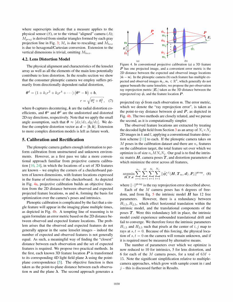
in Fig. 4a, projective calibration builds an objective func-

tion from the 2D distance between observed and expected

projected feature locations, n and n, forming the basis for

optimization over the camera’s poses and intrinsics.

Plenoptic calibration is complicated by the fact that a sin-

gle feature will appear in the imaging plane multiple times,

as depicted in Fig. 4b. A tempting line of reasoning is to

again formulate an error metric based on the 2D distance be-

tween observed and expected feature locations. The prob-

lem arises that the observed and expected features do not

generally appear in the same lenselet images – indeed the

number of expected and observed features is not generally

equal. As such, a meaningful way of finding the “closest”

distance between each observation and the set of expected

features is required. We propose two practical methods. In

the first, each known 3D feature location P is transformed

to its corresponding 4D light field plane λ using the point-

plane correspondence [5]. The objective function is then

taken as the point-to-plane distance between each observa-

tion n and the plane λ. The second approach generates a

�

(a)

�

(b)

Figure 4. In conventional projective calibration (a) a 3D feature

P has one projected image, and a convenient error metric is the

2D distance between the expected and observed image locations

|n−n|. In the plenoptic camera (b) each feature has multiple ex-

pected and observed images nj ,ni ∈ R4, which generally do not

appear beneath the same lenselets; we propose the per-observation

ray reprojection metric |Ei| taken as the 3D distance between the

reprojected ray φi and the feature location P .

projected ray φ from each observation n. The error metric,

which we denote the “ray reprojection error”, is taken as

the point-to-ray distance between φ and P , as depicted in

Fig. 4b. The two methods are closely related, and we pursue

the second, as it is computationally simpler.

The observed feature locations are extracted by treating

the decoded light field from Section 3 as an array of Ni×Nj

2D images in k and l, applying a conventional feature detec-

tion scheme [11] to each. If the plenoptic camera takes on

M poses in the calibration dataset and there are nc features

on the calibration target, the total feature set over which we

optimize is of size ncMNiNj . Our goal is to find the intrin-

sic matrix H , camera poses T , and distortion parameters dwhich minimize the error across all features,

argminH,T ,d

nc∑c=1

M∑m=1

Ni∑s=1

Nj∑t=1

||φs,tc (H,Tm,d),Pc||pt-ray, (8)

where ||·||pt-ray is the ray reprojection error described above.

Each of the M camera poses has 6 degrees of free-

dom, and from Eq. 5 the intrinsic model H has 12 free

parameters. However, there is a redundancy between

H1,5, H2,5, which effect horizontal translation within the

intrinsic model, and the translational components of the

poses T . Were this redundancy left in place, the intrinsic

model could experience unbounded translational drift and

fail to converge. We therefore force the intrinsic parameters

H1,5 and H2,5 such that pixels at the center of i, j map to

rays at s, t = 0. Because of this forcing, the physical loca-

tion of s, t = 0 on the camera will remain unknown, and if

it is required must be measured by alternative means.

The number of parameters over which we optimize is

now reduced to 10 for intrinsics, 5 for lens distortion, and

6 for each of the M camera poses, for a total of 6M +15. Note the significant simplification relative to multiple-

camera approaches, which grow with sample count in i and

j – this is discussed further in Results.

10281028102810301030

As in monocular camera calibration, a Levenberg-

Marquardt or similar optimization algorithm can be em-

ployed which exploits knowledge of the Jacobian. Rather

than deriving the Jacobian here we describe its sparsity pat-

tern and show results based on the trust region reflective

algorithm implemented in MATLAB’s lsqnonlin func-

tion [3]. In practice we have found this to run quickly on

modern hardware, finishing in tens of iterations and taking

in the order of minutes to complete.

The Jacobian sparsity pattern is easy to derive:

each of the M pose estimates will only influence that

pose’s ncNiNj error terms, while all of the 15 in-

trinsic and distortion parameters will affect every er-

ror term. As a practical example, for a checkerboard

with 256 corners, viewed from 16 poses by a camera

with Ni = Nj = 8 spatial samples, there will be

Ne = ncMNiNj = (16)(8)(8)(256) = 262,144 error

terms and Nv = 6M + 15 = 123 optimization vari-

ables. Of the NeNv = 32,243,712 possible interactions,

(15 + 6)Ne = 5,505,024, or about 17% will be non-zero.

5.1. Initialization

The calibration process proceeds in stages: first initial

pose and intrinsic estimates are formed, then an optimiza-

tion is carried out with no distortion parameters, and finally

a full optimization is carried out with distortion parameters.

To form initial pose estimates, we again treat the decoded

light fields across M poses each as an array of Ni ×Nj 2D

images. By passing all the images through a conventional

camera calibration process, for example that proposed by

Heikkila [10], we obtain a per-image pose estimate. Tak-

ing the mean or median within each light field’s Ni × Nj

per-image pose estimates yields M physical pose estimates.

Note that distortion parameters are excluded from this pro-

cess, and the camera intrinsics that it yields are ignored.

In Section 4 we derived a closed-form expression for the

intrinsic matrix H based on the plenoptic camera’s physical

parameters and the parameters of the decoding process (1),

(6). We use these expressions to form the initial estimate

of the camera’s intrinsics. We have found the optimization

process to be insensitive to errors in these initial estimates,

and in cases where the physical parameters of the camera

are unknown, rough estimates may suffice. Automatic esti-

mation of the initial parameters is left as future work.

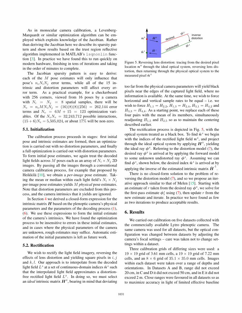
5.2. Rectification

We wish to rectify the light field imagery, reversing the

effects of lens distortion and yielding square pixels in i, jand k, l. Our approach is to interpolate from the decoded

light field LA at a set of continuous-domain indices nA such

that the interpolated light field approximates a distortion-

free rectified light field LR. In doing so, we must select

an ideal intrinsic matrix HR, bearing in mind that deviating

�������

�������������

������

��

Figure 5. Reversing lens distortion: tracing from the desired pixel

location nR through the ideal optical system, reversing lens dis-

tortion, then returning through the physical optical system to the

measured pixel nA

too far from the physical camera parameters will yield black

pixels near the edges of the captured light field, where no

information is available. At the same time, we wish to force

horizontal and vertical sample rates to be equal – i.e. we

wish to force H1,1 = H2,2, H1,3 = H2,4, H3,1 = H4,2 and

H3,3 = H4,4. As a starting point, we replace each of these

four pairs with the mean of its members, simultaneously

readjusting H1,5 and H2,5 so as to maintain the centering

described earlier.

The rectification process is depicted in Fig. 5, with the

optical system treated as a black box. To find nA we begin

with the indices of the rectified light field nR, and project

through the ideal optical system by applying HR, yielding

the ideal ray φR. Referring to the distortion model (7), the

desired ray φR is arrived at by applying the forward model

to some unknown undistorted ray φA. Assuming we can

find φA, shown below, the desired index nA is arrived at by

applying the inverse of the estimated intrinsic matrix H-1

.

There is no closed-form solution to the problem of re-

versing the distortion model (7), and so we propose an iter-

ative approach similar to that of Melen [15]. Starting with

an estimate of r taken from the desired ray φR, we solve for

the first-pass estimate φA1 using (7), then update r from the

new estimate and iterate. In practice we have found as few

as two iterations to produce acceptable results.

6. ResultsWe carried out calibration on five datasets collected with

the commercially available Lytro plenoptic camera. The

same camera was used for all datasets, but the optical con-

figuration was changed between datasets by adjusting the

camera’s focal settings – care was taken not to change set-

tings within a dataset.

Three calibration grids of differing sizes were used: a

19 × 19 grid of 3.61 mm cells, a 19 × 19 grid of 7.22 mm

cells, and an 8 × 6 grid of 35.1 × 35.0 mm cells. Images

within each dataset were taken over a range of depths and

orientations. In Datasets A and B, range did not exceed

20 cm, in C and D it did not exceed 50 cm, and in E it did not

exceed 2 m. Close ranges were favoured in all datasets so as

to maximize accuracy in light of limited effective baseline

10291029102910311031

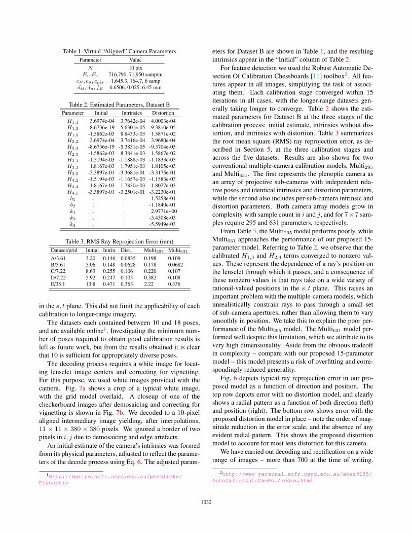
Table 1. Virtual “Aligned” Camera Parameters

Parameter Value

N 10 pix

Fs, Fu 716,790, 71,950 samp/m

cM , cμ, cpix 1,645.3, 164.7, 6 samp

dM , dμ, fM 6.6506, 0.025, 6.45 mm

Table 2. Estimated Parameters, Dataset B

Parameter Initial Intrinsics Distortion

H1,1 3.6974e-04 3.7642e-04 4.0003e-04

H1,3 -8.6736e-19 -5.6301e-05 -9.3810e-05

H1,5 -1.5862e-03 8.8433e-03 1.5871e-02

H2,2 3.6974e-04 3.7416e-04 3.9680e-04

H2,4 -8.6736e-19 -5.3831e-05 -9.3704e-05

H2,5 -1.5862e-03 8.3841e-03 1.5867e-02

H3,1 -1.5194e-03 -1.1888e-03 -1.1833e-03

H3,3 1.8167e-03 1.7951e-03 1.8105e-03

H3,5 -3.3897e-01 -3.3681e-01 -3.3175e-01

H4,2 -1.5194e-03 -1.1657e-03 -1.1583e-03

H4,4 1.8167e-03 1.7830e-03 1.8077e-03

H4,5 -3.3897e-01 -3.2501e-01 -3.2230e-01

b1 . . 1.5258e-01

b2 . . -1.1840e-01

k1 . . 2.9771e+00

k2 . . -3.4308e-03

k3 . . -5.5949e-03

Table 3. RMS Ray Reprojection Error (mm)

Dataset/grid Initial Intrin. Dist. Multi295 Multi631

A/3.61 3.20 0.146 0.0835 0.198 0.109

B/3.61 5.06 0.148 0.0628 0.178 0.0682

C/7.22 8.63 0.255 0.106 0.220 0.107

D/7.22 5.92 0.247 0.105 0.382 0.108

E/35.1 13.8 0.471 0.363 2.22 0.336

in the s, t plane. This did not limit the applicability of each

calibration to longer-range imagery.

The datasets each contained between 10 and 18 poses,

and are available online1. Investigating the minimum num-

ber of poses required to obtain good calibration results is

left as future work, but from the results obtained it is clear

that 10 is sufficient for appropriately diverse poses.

The decoding process requires a white image for locat-

ing lenselet image centers and correcting for vignetting.

For this purpose, we used white images provided with the

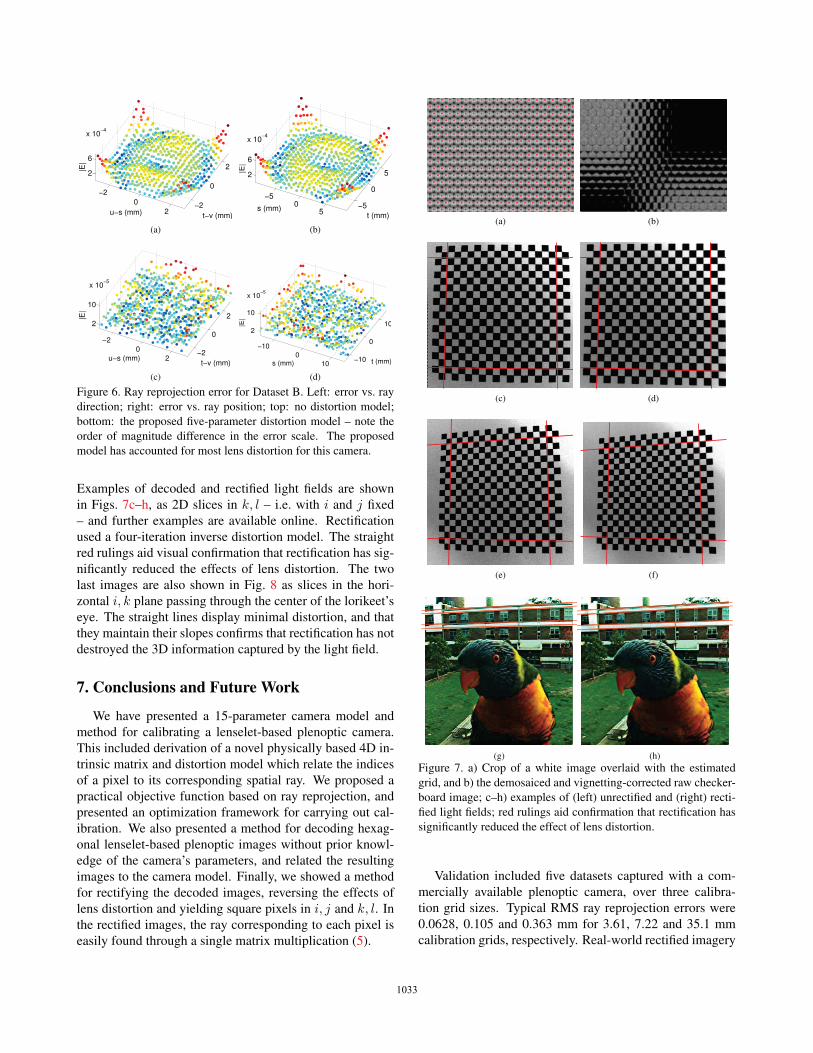
camera. Fig. 7a shows a crop of a typical white image,

with the grid model overlaid. A closeup of one of the

checkerboard images after demosaicing and correcting for

vignetting is shown in Fig. 7b. We decoded to a 10-pixel

aligned intermediary image yielding, after interpolations,

11 × 11 × 380 × 380 pixels. We ignored a border of two

pixels in i, j due to demosaicing and edge artefacts.

An initial estimate of the camera’s intrinsics was formed

from its physical parameters, adjusted to reflect the parame-

ters of the decode process using Eq. 6. The adjusted param-

1http://marine.acfr.usyd.edu.au/permlinks/Plenoptic

eters for Dataset B are shown in Table 1, and the resulting

intrinsics appear in the “Initial” column of Table 2.

For feature detection we used the Robust Automatic De-

tection Of Calibration Chessboards [11] toolbox2. All fea-

tures appear in all images, simplifying the task of associ-

ating them. Each calibration stage converged within 15

iterations in all cases, with the longer-range datasets gen-

erally taking longer to converge. Table 2 shows the esti-

mated parameters for Dataset B at the three stages of the

calibration process: initial estimate, intrinsics without dis-

tortion, and intrinsics with distortion. Table 3 summarizes

the root mean square (RMS) ray reprojection error, as de-

scribed in Section 5, at the three calibration stages and

across the five datasets. Results are also shown for two

conventional multiple-camera calibration models, Multi295and Multi631. The first represents the plenoptic camera as

an array of projective sub-cameras with independent rela-

tive poses and identical intrinsics and distortion parameters,

while the second also includes per-sub-camera intrinsic and

distortion parameters. Both camera array models grow in

complexity with sample count in i and j, and for 7×7 sam-

ples require 295 and 631 parameters, respectively.

From Table 3, the Multi295 model performs poorly, while

Multi631 approaches the performance of our proposed 15-

parameter model. Referring to Table 2, we observe that the

calibrated H1,3 and H2,4 terms converged to nonzero val-

ues. These represent the dependence of a ray’s position on

the lenselet through which it passes, and a consequence of

these nonzero values is that rays take on a wide variety of

rational-valued positions in the s, t plane. This raises an

important problem with the multiple-camera models, which

unrealistically constrain rays to pass through a small set

of sub-camera apertures, rather than allowing them to vary

smoothly in position. We take this to explain the poor per-

formance of the Multi295 model. The Multi631 model per-

formed well despite this limitation, which we attribute to its

very high dimensionality. Aside from the obvious tradeoff

in complexity – compare with our proposed 15-parameter

model – this model presents a risk of overfitting and corre-

spondingly reduced generality.

Fig. 6 depicts typical ray reprojection error in our pro-

posed model as a function of direction and position. The

top row depicts error with no distortion model, and clearly

shows a radial pattern as a function of both direction (left)

and position (right). The bottom row shows error with the

proposed distortion model in place – note the order of mag-

nitude reduction in the error scale, and the absence of any

evident radial pattern. This shows the proposed distortion

model to account for most lens distortion for this camera.

We have carried out decoding and rectification on a wide

range of images – more than 700 at the time of writing.

2http://www-personal.acfr.usyd.edu.au/akas9185/AutoCalib/AutoCamDoc/index.html

10301030103010321032

−20

2−2

0

22

6

u−s (mm)

|E|

t−v (mm)

x 10−4

(a)

−50

5−5

0

52

6

t (mm)

|E|

s (mm)

x 10−4

(b)

−20

2−2

0

22

10

t−v (mm)

|E|

u−s (mm)

x 10−5

(c)

s (mm)

x 10

−100

10 −10

0

102

10

t (mm)

|E|

−5

(d)

Figure 6. Ray reprojection error for Dataset B. Left: error vs. ray

direction; right: error vs. ray position; top: no distortion model;

bottom: the proposed five-parameter distortion model – note the

order of magnitude difference in the error scale. The proposed

model has accounted for most lens distortion for this camera.

Examples of decoded and rectified light fields are shown

in Figs. 7c–h, as 2D slices in k, l – i.e. with i and j fixed

– and further examples are available online. Rectification

used a four-iteration inverse distortion model. The straight

red rulings aid visual confirmation that rectification has sig-

nificantly reduced the effects of lens distortion. The two

last images are also shown in Fig. 8 as slices in the hori-

zontal i, k plane passing through the center of the lorikeet’s

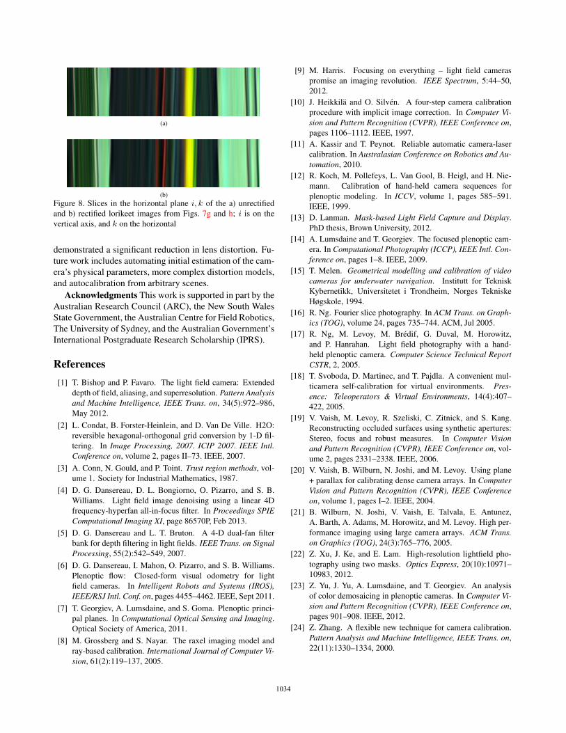
eye. The straight lines display minimal distortion, and that

they maintain their slopes confirms that rectification has not

destroyed the 3D information captured by the light field.

7. Conclusions and Future Work

We have presented a 15-parameter camera model and

method for calibrating a lenselet-based plenoptic camera.

This included derivation of a novel physically based 4D in-

trinsic matrix and distortion model which relate the indices

of a pixel to its corresponding spatial ray. We proposed a

practical objective function based on ray reprojection, and

presented an optimization framework for carrying out cal-

ibration. We also presented a method for decoding hexag-

onal lenselet-based plenoptic images without prior knowl-

edge of the camera’s parameters, and related the resulting

images to the camera model. Finally, we showed a method

for rectifying the decoded images, reversing the effects of

lens distortion and yielding square pixels in i, j and k, l. In

the rectified images, the ray corresponding to each pixel is

easily found through a single matrix multiplication (5).

(a) (b)

(c) (d)

(e) (f)

(g) (h)

Figure 7. a) Crop of a white image overlaid with the estimated

grid, and b) the demosaiced and vignetting-corrected raw checker-

board image; c–h) examples of (left) unrectified and (right) recti-

fied light fields; red rulings aid confirmation that rectification has

significantly reduced the effect of lens distortion.

Validation included five datasets captured with a com-

mercially available plenoptic camera, over three calibra-

tion grid sizes. Typical RMS ray reprojection errors were

0.0628, 0.105 and 0.363 mm for 3.61, 7.22 and 35.1 mm

calibration grids, respectively. Real-world rectified imagery

10311031103110331033

(a)

(b)

Figure 8. Slices in the horizontal plane i, k of the a) unrectified

and b) rectified lorikeet images from Figs. 7g and h; i is on the

vertical axis, and k on the horizontal

demonstrated a significant reduction in lens distortion. Fu-

ture work includes automating initial estimation of the cam-

era’s physical parameters, more complex distortion models,

and autocalibration from arbitrary scenes.

Acknowledgments This work is supported in part by the

Australian Research Council (ARC), the New South Wales

State Government, the Australian Centre for Field Robotics,

The University of Sydney, and the Australian Government’s

International Postgraduate Research Scholarship (IPRS).

References[1] T. Bishop and P. Favaro. The light field camera: Extended

depth of field, aliasing, and superresolution. Pattern Analysisand Machine Intelligence, IEEE Trans. on, 34(5):972–986,

May 2012.

[2] L. Condat, B. Forster-Heinlein, and D. Van De Ville. H2O:

reversible hexagonal-orthogonal grid conversion by 1-D fil-

tering. In Image Processing, 2007. ICIP 2007. IEEE Intl.Conference on, volume 2, pages II–73. IEEE, 2007.

[3] A. Conn, N. Gould, and P. Toint. Trust region methods, vol-

ume 1. Society for Industrial Mathematics, 1987.

[4] D. G. Dansereau, D. L. Bongiorno, O. Pizarro, and S. B.

Williams. Light field image denoising using a linear 4D

frequency-hyperfan all-in-focus filter. In Proceedings SPIEComputational Imaging XI, page 86570P, Feb 2013.

[5] D. G. Dansereau and L. T. Bruton. A 4-D dual-fan filter

bank for depth filtering in light fields. IEEE Trans. on SignalProcessing, 55(2):542–549, 2007.

[6] D. G. Dansereau, I. Mahon, O. Pizarro, and S. B. Williams.

Plenoptic flow: Closed-form visual odometry for light

field cameras. In Intelligent Robots and Systems (IROS),IEEE/RSJ Intl. Conf. on, pages 4455–4462. IEEE, Sept 2011.

[7] T. Georgiev, A. Lumsdaine, and S. Goma. Plenoptic princi-

pal planes. In Computational Optical Sensing and Imaging.

Optical Society of America, 2011.

[8] M. Grossberg and S. Nayar. The raxel imaging model and

ray-based calibration. International Journal of Computer Vi-sion, 61(2):119–137, 2005.

[9] M. Harris. Focusing on everything – light field cameras

promise an imaging revolution. IEEE Spectrum, 5:44–50,

2012.

[10] J. Heikkila and O. Silven. A four-step camera calibration

procedure with implicit image correction. In Computer Vi-sion and Pattern Recognition (CVPR), IEEE Conference on,

pages 1106–1112. IEEE, 1997.

[11] A. Kassir and T. Peynot. Reliable automatic camera-laser

calibration. In Australasian Conference on Robotics and Au-tomation, 2010.

[12] R. Koch, M. Pollefeys, L. Van Gool, B. Heigl, and H. Nie-

mann. Calibration of hand-held camera sequences for

plenoptic modeling. In ICCV, volume 1, pages 585–591.

IEEE, 1999.

[13] D. Lanman. Mask-based Light Field Capture and Display.

PhD thesis, Brown University, 2012.

[14] A. Lumsdaine and T. Georgiev. The focused plenoptic cam-

era. In Computational Photography (ICCP), IEEE Intl. Con-ference on, pages 1–8. IEEE, 2009.

[15] T. Melen. Geometrical modelling and calibration of videocameras for underwater navigation. Institutt for Teknisk

Kybernetikk, Universitetet i Trondheim, Norges Tekniske

Høgskole, 1994.

[16] R. Ng. Fourier slice photography. In ACM Trans. on Graph-ics (TOG), volume 24, pages 735–744. ACM, Jul 2005.

[17] R. Ng, M. Levoy, M. Bredif, G. Duval, M. Horowitz,

and P. Hanrahan. Light field photography with a hand-

held plenoptic camera. Computer Science Technical ReportCSTR, 2, 2005.

[18] T. Svoboda, D. Martinec, and T. Pajdla. A convenient mul-

ticamera self-calibration for virtual environments. Pres-ence: Teleoperators & Virtual Environments, 14(4):407–

422, 2005.

[19] V. Vaish, M. Levoy, R. Szeliski, C. Zitnick, and S. Kang.

Reconstructing occluded surfaces using synthetic apertures:

Stereo, focus and robust measures. In Computer Visionand Pattern Recognition (CVPR), IEEE Conference on, vol-

ume 2, pages 2331–2338. IEEE, 2006.

[20] V. Vaish, B. Wilburn, N. Joshi, and M. Levoy. Using plane

+ parallax for calibrating dense camera arrays. In ComputerVision and Pattern Recognition (CVPR), IEEE Conferenceon, volume 1, pages I–2. IEEE, 2004.

[21] B. Wilburn, N. Joshi, V. Vaish, E. Talvala, E. Antunez,

A. Barth, A. Adams, M. Horowitz, and M. Levoy. High per-

formance imaging using large camera arrays. ACM Trans.on Graphics (TOG), 24(3):765–776, 2005.

[22] Z. Xu, J. Ke, and E. Lam. High-resolution lightfield pho-

tography using two masks. Optics Express, 20(10):10971–

10983, 2012.

[23] Z. Yu, J. Yu, A. Lumsdaine, and T. Georgiev. An analysis

of color demosaicing in plenoptic cameras. In Computer Vi-sion and Pattern Recognition (CVPR), IEEE Conference on,

pages 901–908. IEEE, 2012.

[24] Z. Zhang. A flexible new technique for camera calibration.

Pattern Analysis and Machine Intelligence, IEEE Trans. on,

22(11):1330–1334, 2000.

10321032103210341034