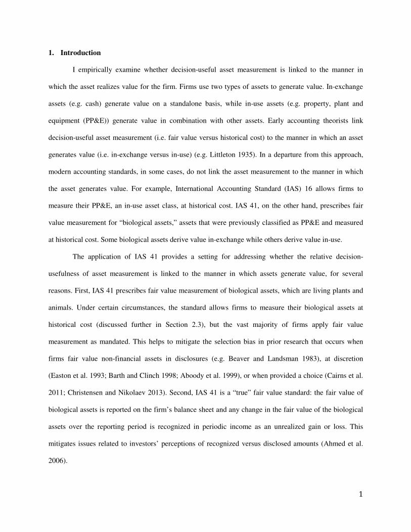
Decision-useful asset measurement and asset

use: Evidence from IAS 41

Adrienna A. Huffman

PhD Candidate

David Eccles School of Business

University of Utah adrienna.huffman@business.utah.edu

October 2013

ABSTRACT: I empirically examine whether decision-useful asset measurement is linked to the way in which the asset realizes value, in a sample of 247 international firms from 42 different countries that adopt International Accounting Standard (IAS) 41. IAS 41 prescribes fair value measurement for biological assets, a class of assets previously classified as PP&E and measured at cost. I find that when firms measure their biological assets consistent with the way in which the assets generate value, the explanatory power from value relevance estimations of stock price and returns, and from forecasting models of operating cash flows and operating income are all significantly higher relative to firms that measure their biological assets inconsistent with their use. My findings provide support for early accounting theory that links decision-useful asset measurement to the way in which the asset generates value (e.g. Littleton 1935; May 1936), current asset measurement frameworks, and the International Accounting Standards Board’s (2013) recent revisions to the asset measurement section of its conceptual framework. Key words: International accounting; asset measurement; fair value accounting; decision-useful information; business valuation.

1

1. Introduction

I empirically examine whether decision-useful asset measurement is linked to the manner in

which the asset realizes value for the firm. Firms use two types of assets to generate value. In-exchange

assets (e.g. cash) generate value on a standalone basis, while in-use assets (e.g. property, plant and

equipment (PP&E)) generate value in combination with other assets. Early accounting theorists link

decision-useful asset measurement (i.e. fair value versus historical cost) to the manner in which an asset

generates value (i.e. in-exchange versus in-use) (e.g. Littleton 1935). In a departure from this approach,

modern accounting standards, in some cases, do not link the asset measurement to the manner in which

the asset generates value. For example, International Accounting Standard (IAS) 16 allows firms to

measure their PP&E, an in-use asset class, at historical cost. IAS 41, on the other hand, prescribes fair

value measurement for “biological assets,” assets that were previously classified as PP&E and measured

at historical cost. Some biological assets derive value in-exchange while others derive value in-use.

The application of IAS 41 provides a setting for addressing whether the relative decision-

usefulness of asset measurement is linked to the manner in which assets generate value, for several

reasons. First, IAS 41 prescribes fair value measurement of biological assets, which are living plants and

animals. Under certain circumstances, the standard allows firms to measure their biological assets at

historical cost (discussed further in Section 2.3), but the vast majority of firms apply fair value

measurement as mandated. This helps to mitigate the selection bias in prior research that occurs when

firms fair value non-financial assets in disclosures (e.g. Beaver and Landsman 1983), at discretion

(Easton et al. 1993; Barth and Clinch 1998; Aboody et al. 1999), or when provided a choice (Cairns et al.

2011; Christensen and Nikolaev 2013). Second, IAS 41 is a “true” fair value standard: the fair value of

biological assets is reported on the firm’s balance sheet and any change in the fair value of the biological

assets over the reporting period is recognized in periodic income as an unrealized gain or loss. This

mitigates issues related to investors’ perceptions of recognized versus disclosed amounts (Ahmed et al.

2006).

2

Third, there is variation in both the extent to which biological assets derive value in-use versus in-

exchange, and the extent to which firms employ fair value versus historical cost measurement, for reasons

discussed above. Some firms measure their biological assets at historical cost, whether they derive value

in-use versus in-exchange, while other firms measure their biological assets at fair value, whether the

assets derive value in-use or in-exchange. This allows for cross-sectional comparison of biological asset-

groups where the asset measurement is consistent with the assets’ use, versus when it is not. I investigate

the relative decision-usefulness of consistent versus inconsistent measurement by asset use (hereafter,

consistent and inconsistent samples) in a sample of 247 international firms from 42 countries that adopt

IAS 41.

In their joint conceptual framework for financial reporting, the Financial Accounting Standards

Board (FASB) and the International Accounting Standards Board (IASB) characterize financial

information as decision-useful if it aids users in forecasting the amount, timing and uncertainty of the

reporting entity’s future cash flows (¶OB3-¶OB4, IASB 2010). I adopt this characterization of decision-

useful information, and focus on the decision-usefulness of financial reporting information to users

interested in assessing the value of a going concern. For expositional ease, I refer to such users as

“investors.”1

I adopt a multi-pronged approach to assess decision-usefulness. First, I compare the explanatory

power from value relevance regressions of stock price and returns for the consistent and inconsistent

measurement samples. Second, I examine the explanatory power of mechanical forecasting models of

operating cash flows and operating income. I find that measurement consistent with asset use provides

investors with relatively more decision-useful information than asset measurement that is inconsistent

1 I recognize that the information needs of some users of financial reporting information are driven by economic decisions that are not informed by an assessment of firm value. I focus on the information needs of users interested in assessing firm value because a rigorous consideration of the information needs of all users is impractical. Moreover, I believe the users I focus on comprise an important set. This is supported by Dichev et al. (2012), who find that 94.7% of the public company CFOs they surveyed identify valuation as the primary reason earnings are important to users.

3

with asset use. This finding provides support for early accounting theory that links decision-useful asset

measurement to the way in which the asset generates value (e.g. Littleton 1935; May 1936). Specifically,

I find that the adjusted R-squared for the value relevance price and return models, and the mechanical

forecasting models of operating cash flows and operating income are all significantly higher when firms

measure their biological assets consistent with their use relative to when they do not.

My findings support an asset measurement framework that links decision-useful asset

measurement to the manner in which the assets realize value for the firm, and suggest that a measurement

basis that violates the link to asset use provides investors with relatively less decision-useful information

to assess firm value. Further, my findings support the IASB’s recent revisions to the measurement section

of its conceptual framework. Specifically, the IASB (2013) states that the relevance and selection of a

particular measurement basis depends on how the asset contributes to the entity’s future cash flows and

this occurs either directly (i.e. in-exchange) or in combination with other assets (i.e. in-use) (¶6.16). My

results provide empirical support for this assertion. Moreover, my results provide an alternative

explanation as to why firms rejected fair value measurement for non-financial assets upon adoption of

International Financial Reporting Standards (IFRS). Cairns et al. (2011) and Christensen and Nikolaev

(2013) find that few firms elect to measure their non-financial, in-use assets, in particular PP&E, at fair

value upon adoption of IFRS. If firms seek to provide investors with decision-useful information, then

fair valuing PP&E, an in-use asset, would not provide investors with relatively more decision-useful

information, and therefore, would not justify the cost of adoption.

Much of the prior literature examining fair value measurement investigates whether fair value is

sufficiently reliable to be decision-useful to investors, beyond measurement at historical cost.2 This

relative reliability perspective differs from a business valuation perspective, which links decision-useful

asset measurement to the manner in which the asset realizes value, not on the reliability of the measure.

The latter perspective, which has its roots in early accounting theory (e.g. Littleton 1935; May 1936),

2 See, for example, among others: Easton et al. 1993; Barth 1994a,b; Bernard et al. 1995; Barth et al. 1996; Barth and Clinch (1998); Aboody et al. 1999; Song et al. 2010.

4

underpins a recent framework for asset measurement proposed in Botosan and Huffman (2013). In

contrast to the relative reliability research, the business valuation perspective predicts that fair value

information is more decision-useful for in-exchange assets than in-use assets, regardless of relative

reliability.

My findings are of interest to standard setters, academics and practitioners alike. At present, the

FASB and the IASB lack a systematic framework to guide asset measurement standards.3 As a result,

asset measurement guidance continues to be a hotly contested standard setting issue and inconsistencies

exist across standards.4 Thus, a framework to guide standard setters’ asset measurement choices and to

support high-quality, consistent standard setting is greatly needed. Moreover, by understanding which

asset measurement is useful to investors in determining firm value, standard setters are better positioned

to understand cost-benefit tradeoffs and how to improve the effectiveness of financial statement

disclosures, which is the primary objective of the FASB’s disclosure framework project (FASB 2012). I

seek to supplement and contribute to the extant literature by providing evidence regarding the link

between decision-useful asset measurement and the manner in which assets realize value.

The remainder of my paper is organized as follows. Section 2 develops the hypothesis, related

literature, and IAS 41 background. Section 3 explains the research design. Section 4 describes the data.

Section 5 presents the results. Section 6 concludes.

2. Hypothesis Development, Related Literature, and Background

This study relates to two primary streams of literature. The first stream of literature develops asset

measurement frameworks from a valuation approach, and suggests that a uniform measurement basis may

not provide investors with all information necessary for business valuation. A second stream provides

evidence on the value relevance of fair value measurement for in-exchange and in-use assets. This paper

3 For example, the opening paragraph of the measurement section from the IASB’s (2013) discussion paper of its conceptual framework states: “The existing Conceptual Framework provides little guidance on measurement and when particular measurement should be used” (¶6.1). 4 The objective of the IASB and FASB’s joint project on an improved conceptual framework for financial reporting is “…for their standards to be clearly based on consistent principles. To be consistent, principles must be rooted in fundamental concepts rather than a collection of conventions” (as quoted in Milburn 2012; from ¶P4, IASB 2008).

5

empirically tests the link between these two streams of literature by examining whether decision-useful

asset measurement is linked to the manner in which the asset generates value for the firm.

2.1 A Business Valuation Framework for Asset Measurement

The asset measurement framework I adopt suggests that the asset measurement that is decision-

useful to investors is a function of how the asset is expected to realize value for the firm. Value realization

occurs via two mechanisms: in-exchange or in-use (Botosan and Huffman 2013, hereafter BH). In-

exchange assets are expected to realize their contribution to firm value on a standalone basis in exchange

for cash or other economically valuable assets and derive no additional value from being used in

combination with other assets. BH show that fair value measurement of in-exchange assets provides

investors with the most decision-useful information to assess the value in-exchange assets generate for the

firm.

In contrast, in-use assets are expected to realize their contribution to firm value employed in

combination with other assets. This combination of assets can be referred to as a “cash generating unit.”

The in-use value of the cash generating unit is expected to exceed the sum of the individual assets’

standalone exchange values (Fortgang and Mayer 1985), leading BH to conclude that the fair value

measurement of individual in-use assets does not provide investors with decision-useful information.

Feltham and Ohlson (hereafter FO, 1995) model firm value as separately attributable to firm’s

financing and operating activities. BH adapt the valuation model presented in FO, and conclude that a

firm’s equity value can also be modeled as firm value attributable to value generated by in-exchange

assets and value generated by in-use assets. Specifically, equity value (Pt) is equal to a firm’s net in-

exchange assets measured at market value plus the discounted expected value of the firm’s infinite

horizon expected future cash flows generated from in-use assets, net of investments in those assets. The

relevant equation is shown below:

�� = ��� +∑ ���� �̃����

���� (1)

Where: ��� = in-exchange assets net of financial obligations, measured at market value, date t. � = one plus the risk-free interest rate.

6

�� = expectation formed based on available information, date t. �� = cash flows realized from in-use assets, net of investments in those activities, date t.

BH conclude that the discounted expected value of the firm’s infinite horizon expected future

cash flows generated from in-use assets, net of investments in those assets, is equal to the book value of

the in-use assets at date t plus goodwill. Specifically:

∑ ���� �̃����

���� = ��� + �� (2)

Where: ��� = in-use assets, net of operating liabilities, date t. �� = unrecorded goodwill, i.e. �� ≡ �� − ���.

All other variables are defined above.

Goodwill in (2),��, represents the incremental value in-use assets create for the firm when used

as part of a cash generating unit. This value is incremental to the standalone exchange values of the in-use

assets. Further, it is not possible to meaningfully allocate the goodwill to individual in-use assets because

this incremental value is a joint value created by the assets used in combination. Consequently, the in-use

value for an asset cannot be meaningfully estimated independent of the other assets in the cash generating

unit.

For example, it is possible to estimate the present value of the future cash flows generated by

machinery, materials, and labor (a cash generating unit), which produces a product sold to produce net

cash inflows for the firm. The resulting value is expected to exceed the sum of the individual market

exchange values of the machinery, materials and labor but that excess value cannot be meaningfully

attributed to any individual asset(s) since it is created by using the assets in combination with one another.

From equations (1) and (2), it becomes apparent that from a business valuation perspective

investors require the following information. First, they require sufficient information to allow them to

assess the market values of in-exchange assets and financial obligations. Second, investors require

sufficient information to allow them to form reliable expectations regarding the future cash flows to be

realized from in-use assets, net of investments in those activities. In particular, (2) demonstrates that the

asset measurement that would faithfully represent the value of an in-use asset is value-in-use, but because

this value is only realized in combination with the firm’s other productive assets, it is not determinable on

7

a standalone basis. Consequently, BH conclude that fair value measurement will provide investors with

decision-useful information to forecast the value in-exchange assets generate, but fair value measurement

will not provide decision-useful information for investors forecasting the value in-use assets create. I

empirically test the validity of these predictions using the adoption of IAS 41.

The predictions from the BH model are consistent with the IASB’s (2013) recent revisions to the

measurement section of its conceptual framework. The IASB (2013) believes that the relevance and

selection of a particular measurement basis depends on how the asset contributes to the entity’s future

cash flows (¶6.16). Some assets contribute cash flows directly (i.e. derive value in-exchange) while other

assets are used in combination with other assets (i.e. derive value in-use) (¶6.16a-¶6.16b, IASB 2013).

The IASB (2013) believes that users of financial statements are likely to find information about the

asset’s current market price useful in assessing in-exchange assets’ contribution to firm value but for in-

use assets, current market prices may not provide investors with relevant information (¶6.16a-¶6.16b).

Instead, for in-use assets, the IASB (2013) states, users will often use cost-based information about

transactions and past margins to assess how the assets will contribute to the entity’s future cash flows

(¶6.16b). I test these assertions empirically to investigate whether decision-useful asset measurement is

linked to the manner in which the asset generates value.

Finally, other asset measurement frameworks that take a business valuation perspective reach

similar conclusions to BH. Specifically, Nissim and Penman (2008) argue that fair value accounting is

sufficient for reporting to shareholders only when the firm does not add value to the input through its

business model (Principle 1). A firm does not add value to the input through its business model when the

asset is bought and sold in the same market, i.e. an in-exchange asset. Otherwise, Nissim and Penman

(2008) maintain that historical cost accounting is designed for business models where the firm transforms

inputs to add value, i.e. in-use assets. In addition, a measurement framework developed by the ICAEW

(2010), a UK-based, global organization of accounting professionals, advocates for market exchange

values for assets that are not being used or created within the firm (¶3.2), i.e. assets that derive value in-

exchange. Otherwise, the ICAEW (2010) framework also advocates for historical cost accounting as the

8

most relevant measurement basis when the firm’s business model is to transform inputs so as to create

new assets or services as outputs.

2.2 Relation to Prior Literature

Consistent with the BH framework, prior research has repeatedly established the decision-

usefulness of fair value measurement for a specific class of in-exchange assets: financial securities.5

Moreover, these findings extend to investors’ use of fair value measurement information for in-exchange

assets under all three levels of the fair value measurement hierarchy defined by Statement of Financial

Accounting Standard (SFAS) 157: market exchange value (Level 1), market exchange value adjusted for

specific asset characteristics (Level 2), and fair value measured using valuation techniques (Level 3)

(Kolev 2009; Song et al. 2010). Accordingly, the decision-usefulness of fair value information is not

simply a function of measurement reliability.

Research regarding equity investors’ use of fair value measurement for in-use assets, however, is

burdened by the lack of measurement variation across in-use asset classes. Accordingly, early research

examining investors’ use of fair value information for in-use assets examines disclosed current cost

estimates for firms’ PP&E required under SFAS 33. This research fails to find that current cost

disclosures are value relevant (e.g. Beaver and Landsman 1983; Beaver and Ryan 1985; Bernard and

Ruland 1987; Hopwood and Schaefer 1989; Lobo and Song 1989). The lack of relevance, however, could

be attributable to investors’ perceptions of disclosed values as less reliable or relevant than recognized

amounts (e.g. Ahmed et al. 2006).

Later research examining investors’ use of fair value measurement for in-use assets employs

settings in which U.K. and Australian firms made discretionary and infrequent revaluations to their

tangible long-lived assets. The research findings are mixed. Easton et al. (1993) find that Australian

firms’ asset revaluations of in-use assets are value relevant, but not associated with the firms’ future

5 These studies consistently find that investors perceive fair value estimates for financial securities as more value relevant than historical cost amounts: Barth 1994a, b; Ahmed and Takeda 1995; Bernard et al. 1995; Petroni and Whalen 1995; Barth et al. 1996; Eccher et al. 1996; Nelson 1996.

9

return performance. Barth and Clinch (1998) find that the value relevance of Australian firms’

revaluations of long-lived assets depends on both the firm’s industry and asset class after controlling for

measurement at historical coast (see Table IV). Aboody et al. (1999) find that U.K. firms’ revaluation

activity is significantly associated with the firms’ future operating performance. As Christensen and

Nikolaev (2013) argue, however, a problem with discretionary asset revaluations is that managers decide

to revalue ex-post and therefore may revalue for a host of reasons that are unrelated to providing investors

with decision-useful information, i.e. when they need to manage reported performance.

Further, few financial accounting standards mandate measurement of in-use assets at fair value;

international accounting standards provide firms with a choice of measurement at cost or fair value for

several classes of in-use assets.6 Accordingly, more recent research on fair value measurement of in-use

assets examines firms’ measurement choice for non-financial assets upon adoption of IFRS. Both Cairns

et al. (2011) and Christensen and Nikolaev (2013) find that few U.K., Australian, and German firms

choose to measure their non-financial assets at fair value upon adoption of IFRS. In particular,

Christensen and Nikolaev (2013) find that firms continue to measure their investment property at fair

value, consistent with the prior U.K. GAAP standard SSAP 19, but almost exclusively choose cost

measurement for intangibles and PP&E asset classes (i.e. in-use assets).

This result contradicts Christensen and Nikolaev’s original hypothesis that upon IFRS adoption,

most firms would move towards fair value measurement for non-financial assets. Once more, the lack of

an asset measurement framework that predicts when fair value provides investors with decision-useful

information becomes apparent. Consequently, empirically assessing the relevance, or lack thereof, of fair

value measurement for in-use assets is challenging.

2.3 IAS 41

6 U.K. GAAP mandated fair value measurement of investment property, an in-use asset, pre-IFRS. Upon adoption of IFRS, however, firms were given a choice to measure investment property at cost or fair value under IAS 40. Almost all UK, and German, real estate firms, with large holdings of investment property, continued to measure the assets at fair value (Muller et al. 2011). Again, this provides little variation in asset measurement across in-use assets.

10

The recent passage of IAS 41 offers a unique setting to test investors’ use of fair value

measurement for in-exchange and in-use assets because it prescribes fair value measurement for

biological assets, an asset class that prior to IFRS was not governed by any unified accounting standard.7

In certain situations, IAS 41 allows firms to measure biological assets at historical cost if the firm is able

to demonstrate that the fair value of its biological assets cannot be reliably estimated, i.e. there is a lack of

reliable parameters such as known prices, growth rates or physical volumes of the asset (¶30, IASB

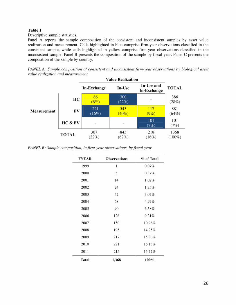
2009). The majority of my sample applies the standard as mandated, however. Specifically, in my sample

28% of the firm-year observations contain biological assets measured at cost, while 64% of the firm-year

observations contain biological assets measured at fair value, and 7% of the firm-year observations

contain a mixture of historical cost and fair value measurement (see Table 1, Panel A). Therefore, IAS 41

provides variation in asset measurement while helping to mitigate the selection bias that occurs when

firms fair value non-financial assets in disclosures, at discretion, or when provided a choice.

IAS 41 prescribes accounting treatment for biological assets, which are living plants and

animals.8 Biological assets are held by firms involved in agricultural activity. Agricultural activities that

produce or employ biological assets include raising livestock, forestry, cropping, cultivating orchards and

plantations, floriculture and aquaculture (¶6, IASB 2009). IAS 41 became effective for annual reporting

periods beginning on or after January 1, 2003, or alternatively, upon adoption of IFRS.

Variation exists in the extent to which firms derive value from biological assets. Specifically, IAS

41 encourages firms to distinguish between “consumable” and “bearer” biological assets in order to

provide information that may help investors in assessing the timing of future cash flows (¶43, IASB

2009). This distinction maps closely into the way in which the biological assets are expected to realize

value for the firm. Consumable biological assets are agricultural produce, like crops, or sold as biological

7 Pre-IFRS, Australian firms had to account for ‘self-generating and re-generating assets’ under AASB 1037, which is similar to (predates) IAS 41. No other countries, however, prescribed accounting treatment for biological assets pre-IFRS adoption. 8 Specifically, IAS 41 prescribes accounting treatment for agricultural activity, or “management by the entity of the biological transformation of living animals and plants (biological assets) for sale, into agricultural produce, or into additional biological assets” (¶IN1, IASB 2009).

11

assets, like commodities (¶44, IASB 2009). Consumable biological assets realize value on a standalone

basis and are therefore closer to in-exchange assets. Bearer biological assets, on the other hand, are self-

regenerating assets, like orchards or timber plantations (¶44, IASB 2009). Bearer biological assets realize

value in combination with other assets and are therefore in-use assets.9

Nevertheless, IAS 41 requires fair value measurement for both in-exchange and in-use biological

assets. Under IAS 41, a firm producing palm oil from oil palm trees measures its oil palm plantations, an

in-use asset, at fair value on the balance sheet, excluding any fair value attributable to the land upon

which the oil palms are physically attached or intangible assets related to the oil palm production (¶2,

IASB 2009). Thus, firms are required to measure and report only the oil palm trees component of the cash

generating unit at fair value. Likewise, a firm that harvests crops for sale, an in-exchange asset, also

measures the crops at fair value every reporting period on the balance sheet, less any costs to sell.

Changes in the fair value of the oil palm plantations or crops (i.e. unrealized holding gains and losses) are

recognized in periodic income (IASB 2009).

Prior to IAS 41, most (albeit not all) firms accounted for biological assets at historical cost.10

Such assets were classified as property, plant and equipment (PP&E) on the balance sheet, and were

subject to impairment analysis. Upon adoption of the standard, most (albeit not all) firms recognize the

fair value of their biological assets on the balance sheet, separate from PP&E. There is no requirement to

disclose measurement at cost in the footnotes, although a handful of firms do so voluntarily.

2.4 Hypothesis

9 Recently, the Asian-Oceanian Standard Setters Group (AOSSG) proposed different accounting treatments for bearer and consumable biological assets because of the differences in the way the asset-types are used by the firm (AOSSG 2011). Specifically, the AOSSG (2011) argues that bearer biological assets are held for income generation (derive value in-use) and therefore should be treated as PP&E, while consumable biological assets are held for sale (derive value in-exchange), and as such should continue to be measured at fair value. In light of the AOSSG paper, the IASB will soon issue a discussion paper that proposes amending IAS 41 with respect to bearer biological assets and allow firms to treat them as PP&E. This means that bearer biological assets will be accounted for under IAS 16 which allows for measurement at cost. 10 As I describe in footnote 6, Australian firms accounted for ‘self-generating and re-generating’ assets at fair value on the balance sheet beginning in fiscal year 2000 under a similar standard that pre-dated IAS 41 (AAB 1037). There are 44 firm-year observations in my sample that account for their biological assets under this standard.

12

In testing the BH framework, I expect that asset measurement linked to the manner in which the

asset derives value will provide investors with more decision-useful information to assess firm value than

asset measurement that is not linked to the manner in which the asset generates value. Consequently, my

main hypothesis examines the relative decision-usefulness of measurement consistent with an asset’s use

versus measurement inconsistent with an asset’s use:

H1: Asset measurement consistent with the way in which an asset realizes value provides

investors with relatively more decision-useful information than asset measurement inconsistent

with the way in which the asset realizes value.

3. Research Design

I adopt a multi-pronged approach to test my hypothesis. First, I compare the explanatory power of

value relevance regressions of stock price and returns for the sample of firms that measure their biological

assets consistent with their use compared to the sample of firms that measure their biological assets

inconsistent with the assets’ use. Second, I examine the explanatory power of mechanical forecasting

models of operating cash flows and operating income for the consistent and inconsistent sample.

I sort firm-year observations into the consistent and inconsistent measurement samples in the

following manner. I employ IAS 41’s definition of consumable and bearer biological assets to represent

in-exchange and in-use biological assets, respectively. To be classified as consistent, I group firm-year

observations where in-exchange biological assets are measured at fair value (221 firm-year observations)

or in-use biological assets are measured at historical cost (300 firm-year observations) (see Table 1, Panel

A). To be classified as inconsistent, I group firm-year observations where in-use biological assets are

measured at fair value (543 firm-year observations) or in-exchange biological assets are measured at

historical cost (86 firm-year observations) (see Table 1, Panel A). For firm-year observations where firms

hold both in-use and in-exchange biological assets, I classify firm-year observations as consistent if the

firm measures its in-exchange biological assets at fair value and its in-use biological assets at historical

cost (101 firm-year observations), and I classify firm-year observations as inconsistent if the firm

measures both its in-use and in-exchange biological assets at fair value (117 firm-year observations) (see

13

Table 1, Panel A). This provides a sample of 622 firm-year observations for the consistent measurement

sample and 746 firm-year observations for the inconsistent measurement sample.

I estimate the models on the full sample, and then separately on the consistent and inconsistent

samples in order to examine the relative explanatory power of the models’ adjusted R-squared. To address

my hypothesis, I test whether the adjusted R-squared from the price, return and forecasting models are

statistically different between the two samples by using a bootstrap method with 1,000 repetitions.

Specifically, the bootstrap method estimates the standard deviation of the adjusted R-squared estimates

from the two samples by randomly sampling 1,000 different sub-samples from each of the consistent and

inconsistent samples. It then estimates the model on each of the 1,000 randomly selected sub-samples.

From the 1,000 different estimations, it calculates the standard deviation of the R-squared estimate. I then

manually calculate the t-statistic from the bootstrap estimate, using unequal variances and sample sizes, to

test if the difference between the adjusted R-squareds is statistically different. The main advantage of

using the bootstrap method to test my hypothesis is that it provides a confidence interval and standard

deviation for the parameter distributions, which helps to assess the stability of the estimated R-squared

results.

I evaluate results in the following manner. If decision-useful asset measurement is linked to the

manner in which the asset realizes value for the firm, then the models estimated on the consistent sample

will have significantly higher adjusted R-squareds across the price, return and future operating

performance models relative to the adjusted R-squareds from the same models estimated on the

inconsistent sample. This would provide evidence supporting my main hypothesis. Specifically, the

evidence would suggest that measurement linked to the way in which the asset realizes value (the

consistent sample) provides investors with relatively more decision-useful information than asset

measurement that is not linked to the way in which the asset realizes value (the inconsistent sample).

3.1 Price and Return Tests

I follow prior value relevance research and examine the association between price (returns), firm

book value, the fair value of the biological assets, income and unrealized gains and losses related to

14

changes in the fair value of the biological assets. In a vein similar to Easton et al. (1993), Barth and

Clinch (1998) and Aboody et al. (1999), I estimate the following model:

��,� =�� + �� !��,� + �" #$��_��&�,� + �'(!_ �)�,� + �*+�,-�,� + .� (3)

where ��,� is the share price for firm i one month following the annual report filing or, alternatively, four

months following the end of the firm’s fiscal year-end; !��,� is the firm’s book value per share at fiscal

year-end, excluding the fair value of the biological assets; #$��_��&�,� is earnings per share at fiscal

year-end excluding any unrealized gains or losses (URGL) related to the biological assets recognized in

income;(!_ �)�,� is the fair value per share of the firm’s biological assets at fiscal year-end excluding

any URGL recognized in income for that fiscal year; and +�,-�,� are the unrealized gains or losses per

share recognized in income related to the change in the fair value of the biological assets over the fiscal

year.

I also include the changes estimation of (3), following Easton et al. (1993), Barth and Clinch

(1998) and Aboody et al. (1999). Specifically, I estimate the following model:

��2�,� = �� + ��34�,� + �"534�,� + �'+�,-�,� + .� (4)

where ��2�,� is the firm i's cumulative 12-month raw return ending the month following the annual report

filing or, alternatively, four months following the end of the firm’s fiscal year-end; 34�,� is the firm’s net

income for the fiscal year, excluding any URGL related to the change in the biological assets over the

fiscal year; 534�,� is the change in net income over the fiscal year; and +�,-�,� is defined above. All

variables are deflated by the log of beginning period market value of equity. I estimate standard errors

clustered by both firm and year for models (3) and (4) because of overlapping return windows and

multiple firm-year price observations. I winsorize the price and return samples at the first and 99th

percentiles to minimize the influence of outliers.

3.2 Mechanical Forecast Models

I examine whether asset measurement linked to asset use influences the ability of a mechanical

forecasting model of firms’ future operating cash flows and operating income. I follow recent work in

15

international accounting research to estimate forecasts of both cash flows and income (e.g. Barth et al.

2012). The operating cash flow model appears below:

7(�,��� = 8 +9�7(�,� +9"34�,� +9'+�,-�,� +.�,� (5)

where net operating cash flows for firm i , 7(���, one, two or three periods ahead of fiscal year t (e.g τ =

1, 2, 3) are a function of: net operating cash flows for fiscal year t, 7(�,�; 34�,� net income for fiscal year t,

excluding any URGL related to the change in the fair value of the biological assets; and +�,-�,� defined

above. All variables are deflated by average total assets.

The operating income model I estimate appears below:

:;_4<����� = 8 +=�:;_4<��,� + =":;_4<��,�� + ='+�,-�,� +.�,� (6)

where operating income for firm i, :;_4<�����, excluding any URGL related to the biological assets, one,

two or three periods ahead of fiscal year t (e.g τ = 1, 2, 3) is a function of: the current period’s operating

income, :;_4<��,�, excluding any URGL related to the change in the fair value of the biological assets;

lagged operating income, :;_4<��,��; and +�,-�,� defined above. I calculate operating income using the

following S&P Capital IQ variables: total revenue less the sum of cost of goods sold; selling, general and

administrative expenses; depreciation and amortization; research and development; and other total

operating expenses. All variables are deflated by average total assets. I include country fixed effects in my

estimations of (5) and (6) to control for the possibility of country-specific intertemporally constant

omitted variables and for consistency with prior research in international accounting settings (i.e. Daske et

al. 2008; Pownall et al. 2013). I cluster standard errors by firm.

4. Data

4.1 Sample Identification and Data Sources

I identify firms that hold biological assets by conducting a word search in the Morningstar

Document Research Global Report’s subscription and in the S&P Capital IQ databases. I search on the

phrase “biological assets.” I supplement this search with a report issued by the Institute of Charted

Accountants of Scotland that lists Australian, UK and French firms that hold biological assets (see

16

Appendix 1, Elad and Herbohn 2011). I restrict the Morningstar and the S&P Capital IQ searches to

annual report filings. I then eliminate firms with biological assets that comprise less than 1% of the firm’s

total assets. I further eliminate firms that have less than $1 million U.S. Dollars (USD) in total assets.

Finally, I restrict my analyses to firms with at least five years of financial statement data available on the

S&P Capital IQ database to eliminate outliers from my estimations that may have undue influence on the

results.

I hand collect the IAS 41 data. Specifically, for each fiscal year in my sample I hand collect the

following amounts: the balance sheet value of the biological assets; any URGL related to the change in

the fair value of the biological assets recognized on the income statement or in the footnote; the

classification of the biological assets as consumable or bearer; and whether the firm measures the

biological assets at fair value or historical cost. I collect all financial statement data from S&P Capital IQ

and I collect all price and return data from Datastream. I select price and return data from the firm’s home

exchange because it contains the longest time-series of market data.11 I pull all financial statement, price,

and return data converted to USD from the respective databases. The hand-collected data, on the other

hand, is reported in the filing currency. I convert the hand collected amounts to USD using the ratio of

S&P Capital IQ’s total assets reported in the firm’s filing currency to S&P Capital IQ’s total assets

reported for the firm in USD to calculate a historical conversion rate. This way I convert the hand-

collected amounts using the same historical conversion rate S&P Capital IQ uses for the other firm

financial statement data. I convert all data to USD for descriptive ease.

4.2 Descriptive Statistics

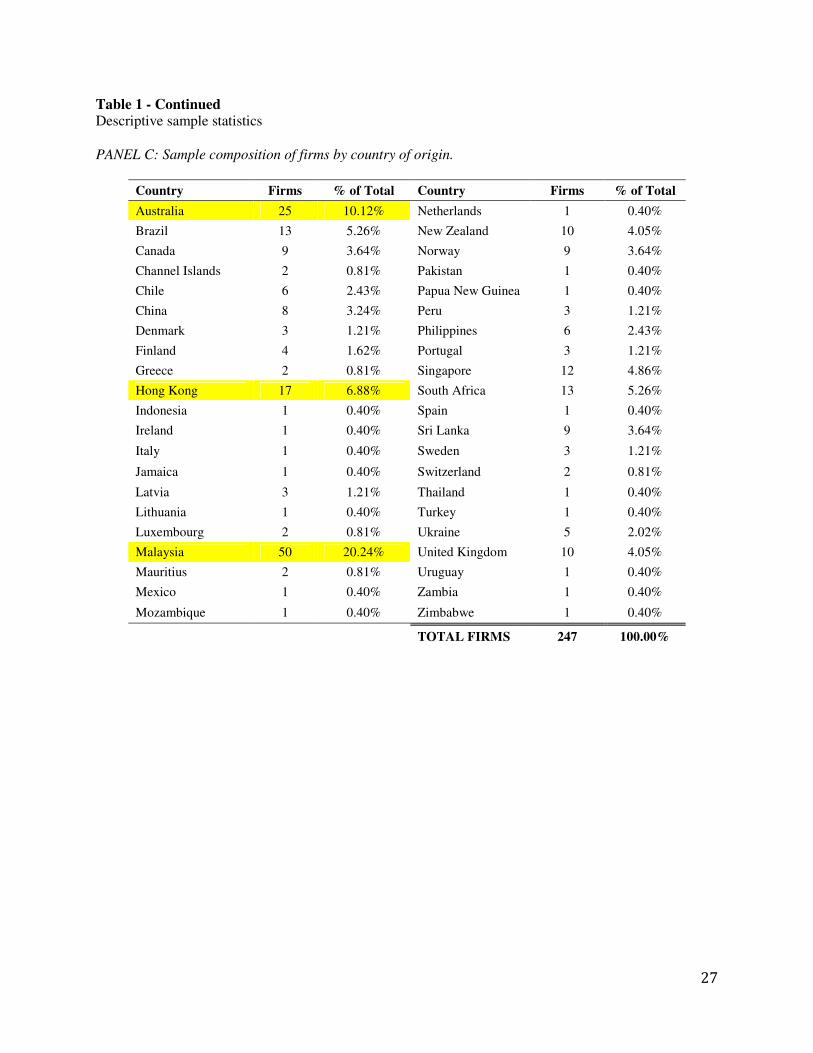
Tables 1 and 2 provide descriptive statistics for the sample. The sample is comprised of firms from 42

different countries (Table 1, Panel C). Approximately 37% of the firms in the sample are located in

Australia, Malaysia or Hong Kong. Moreover, 73% of the firm-year observations are from fiscal years

2007-2011 (Table 1, Panel B). The firm-year observations from 1999-2001 are Australian firms that

11 Fifty-five percent of firms in the sample are cross-listed on a variety of other exchanges.

17

reported the fair value of their re-generating and self-generating assets under the Australian standard

AASB 1037 that pre-dated IAS 41 (see footnotes 7 and 10). I include these observations in the sample

because they provide variation in value realization and asset measurement.

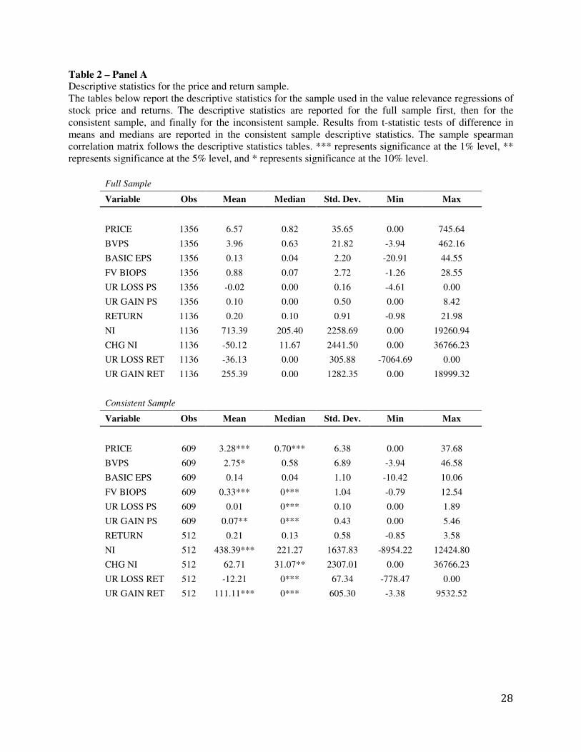
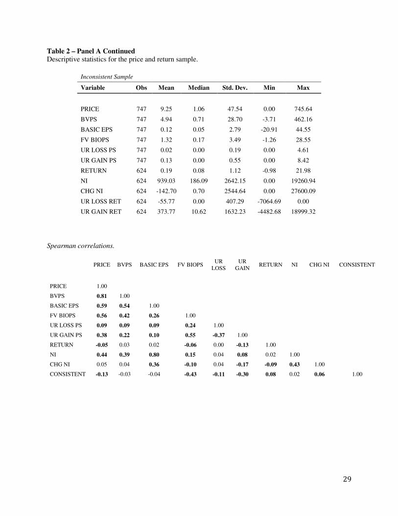
Table 2, Panel A provides descriptive statistics for the price and return samples. Data for the price and

return samples is winsorized at the first and 99th percentiles to reduce the influence of outliers on results.

All data is reported in USD. The inconsistent sample is significantly larger than the consistent sample in

terms of average price ($9.25 vs. $3.28) and book value per share ($4.94 vs. $2.75), and the inconsistent

sample has larger holdings, on average, of biological assets measured at fair value per share ($1.32 vs.

$0.33). Moreover, the inconsistent sample has, on average, significantly larger unrealized gains per share

on its biological assets ($0.13 vs. $0.07). For the return data, which is scaled by the log of beginning

year’s market value of equity, the inconsistent sample has significantly larger net income relative to the

consistent sample, on average.

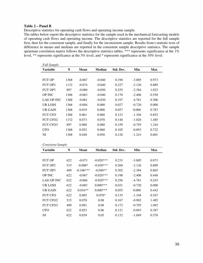
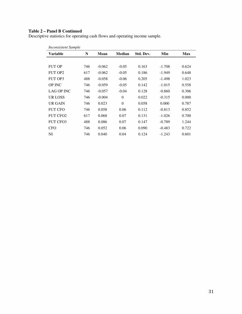
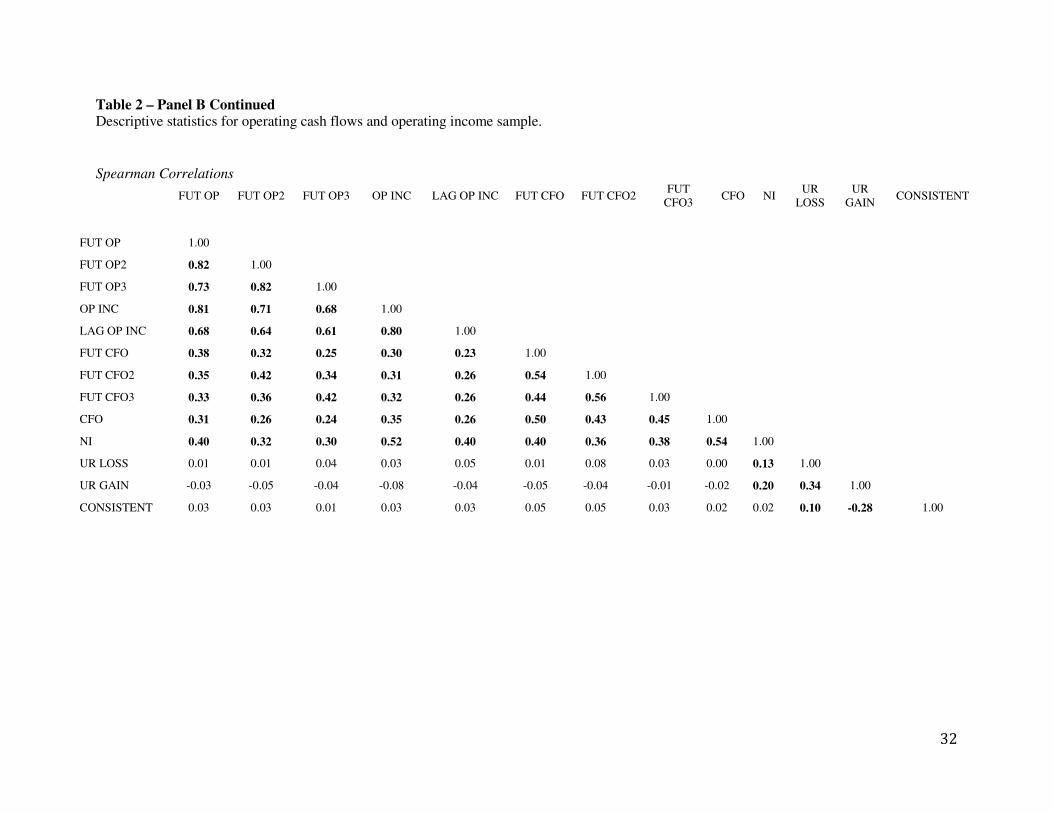
Table 2, Panel B presents the descriptive statistics for the operating cash flows and operating income

forecasting samples. All data is reported in USD. On average, operating income before URGL from the

change in the fair value of the biological assets is negative. This is true for the consistent and inconsistent

samples as well. This may be a result of the firm-years concentrated during fiscal years 2007-2009, which

coincides with the Great Recession. Operating cash flows, on average, are positive as is net income across

both samples. The inconsistent sample is significantly larger in terms of future operating income before

URGL two and three years following the current fiscal year, relative to the consistent sample. The

inconsistent sample also recognizes significantly higher unrealized gains related to the change in the fair

value of their biological assets compared to the consistent sample.

5. Results

5.1 Price and Return Results

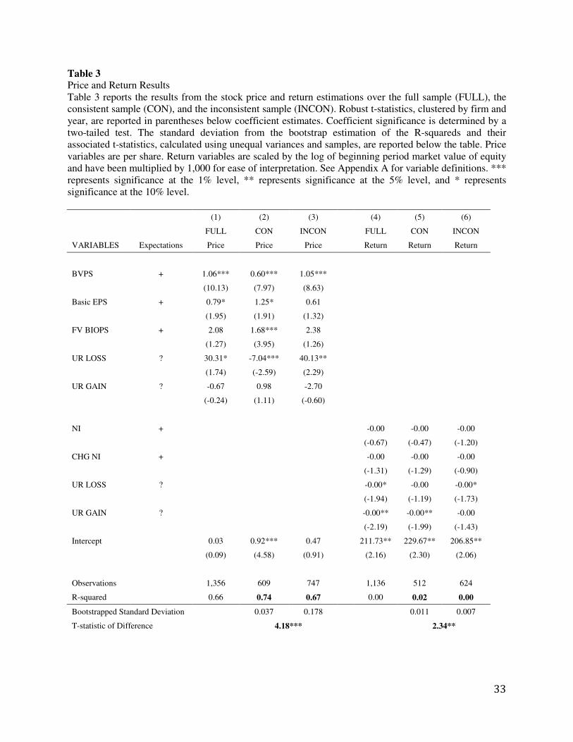
Table 3 columns (1) – (3) present the results from the price estimations, while columns (4)-(6)

present the results from the return estimations. The results from the price model estimated on the full

sample are shown in column (1). Consistent with prior value relevance research, both book value and

18

earnings per share are significantly associated with price. Neither the fair value of the biological assets

nor the URGL are significantly associated price in the full sample, however. Column (2) presents the

results for the price model estimated on the consistent sample and column (3) presents the results of the

price model estimated on the inconsistent sample. For both the consistent and inconsistent sample, book

value per share is significantly associated with price, but only in the consistent sample is earnings per

share and the fair value of the biological assets significantly associated with price.

In all three columns, the unrealized loss associated with the change in the fair value of the

biological assets is significantly associated with price, but in columns (1) and (3), the association is

significantly positive. This result is robust to alternative definitions of basic earnings per share, including

earnings from continuing operations, net income, and earnings before interest and taxes, and it is robust to

the inclusion of firm, country and industry fixed effects. I make no prediction about the sign on the URGL

related to the change in the fair value of the biological assets in any of the remaining analysis. I do this

because it is not clear whether or how URGL will be priced by investors, or map into future financial

statement information. For example, an unrealized gain recognized this period may reverse next year, if

the price used in the measurement of the biological asset declines. Moreover, Dechow et al. (2010) find

that some managers recognize gains on asset securitizations to manage reported performance and to

improve their compensation. Therefore, if some firms use URGL on their biological assets to manage

reported performance, then the relationship between current period URGL and future firm performance

will be ambiguous.

Nevertheless, results from the bootstrapped adjusted R-squared test demonstrate that the adjusted

R-squared from the price model for the consistent sample is significantly larger than the adjusted R-

squared from the inconsistent sample (0.74 vs. 0.67) at the 1% level (t-statistic of 4.18), providing support

for my main hypothesis.

19

Turning to the return results in columns (4)-(6), neither net income nor change in net income is

significantly associated with returns in any of the estimations, contrary to prior value relevance research.12

The lack of significance is robust to the inclusion of year, industry and country fixed effects and to other

definitions of earnings variables. It is possible that the noise in the return data from the concentration of

observations in fiscal years 2007-2009 is driving this result. For the consistent sample, the unrealized gain

associated with the change in biological assets is significantly, but negatively associated with firm returns,

but not at an economically significant magnitude. For the inconsistent sample, the unrealized loss

associated with the change in biological assets is significantly, and negatively associated with firm

returns, but not at an economically significant magnitude.

Results from the bootstrapped R-squared tests continue to provide evidence in support of my

main hypothesis. The bootstrapped R-squared for the consistent sample is significantly higher than the

inconsistent sample (0.02 vs. 0.00) at the 5% level (t-statistic of 2.34).

Overall, the results from the price and return value relevance regressions provide support for my

main hypothesis, that measurement consistent with asset use provides investors with relatively more

decision-useful information than measurement inconsistent with asset use.

5.2 Cash Flow and Operating Income Forecasting Results

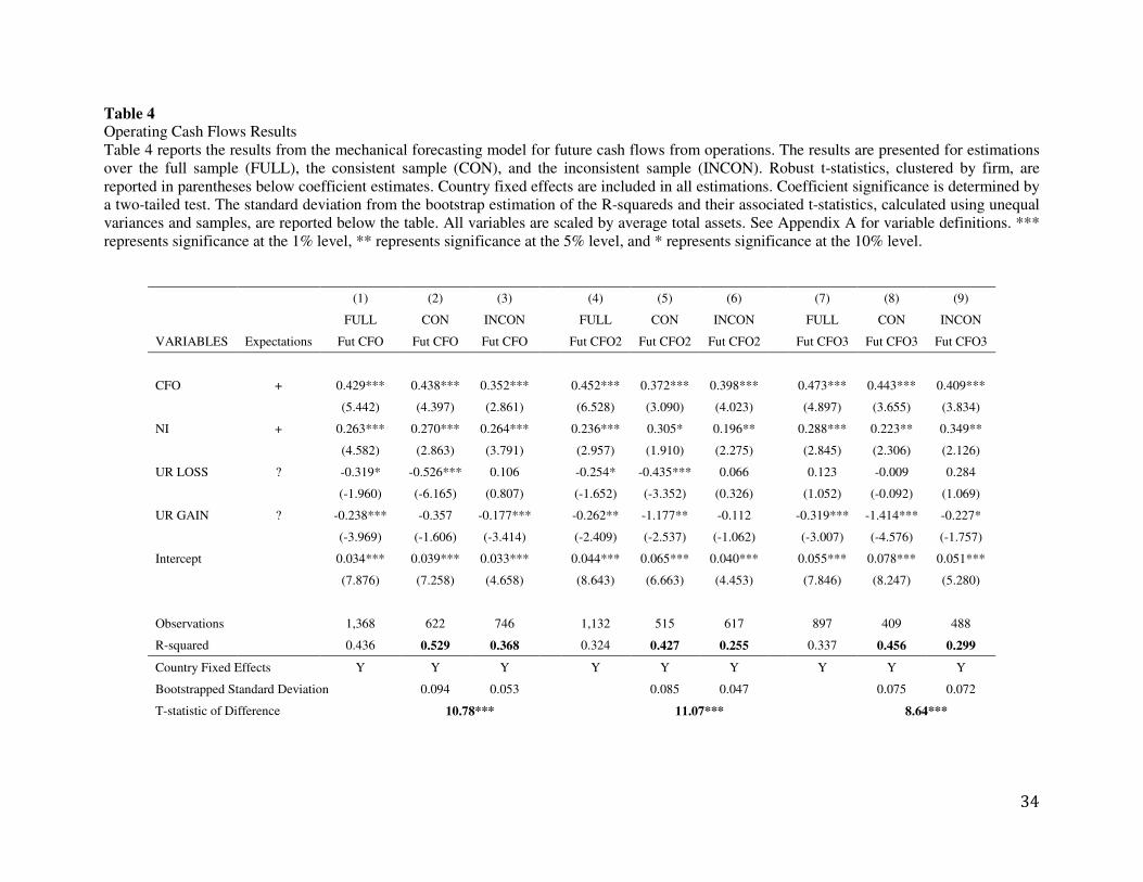
Table 4 presents the results from the mechanical forecasting models for future cash flows from

operations. Columns (1)-(3) present the results for future cash flows one period into the future, while

columns (4)-(6) and columns (7)-(9) present the results for future cash flows two and three periods into

the future, respectively.

Over all estimations, current period cash flow from operations and net income, excluding the

URGL from the biological assets, are significantly associated with future cash flows across all future

period horizons. For the consistent sample, the unrealized loss on biological assets is significantly and

negatively associated with future cash flows one and two periods into the future, while the unrealized loss

12 All return coefficients have been multiplied by 1,000 for ease of interpretation.

20

is never significantly associated with future operating cash flows for the inconsistent sample. On the other

hand, the unrealized gain on the biological assets is significantly and negatively associated with future

cash flows across the board. This result is robust to alternative specifications of the cash flow forecasting

regression and to the inclusion of year and industry fixed effects.

Nonetheless, results from the bootstrapped R-squared tests continue to provide support for my

main hypothesis. Specifically, for all horizons of the operating cash flows forecasting results, the adjusted

R-squareds for the consistent sample are significantly higher, at the 1% level, than the adjusted R-

squareds from the inconsistent sample for the models of: future operating cash flows (0.53 vs. 0.37, t-

statistic of 10.78); future operating cash flows two periods into the future (0.43 vs. 0.25, t-statistic of

11.07); and future operating cash flows three periods into the future (0.46 vs. 0.30, t-statistic of 8.64).

Finally, Table 5 presents the results from the mechanical forecasting models for operating

income. Columns (1)-(3) present the results for future operating income one period into the future, while

columns (4)-(6) and columns (7)-(9) present the results for future operating income two and three periods

into the future, respectively. Over all estimations, current period operating income, excluding the URGL

from the biological assets, is significantly associated with future operating income across all horizons.

The unrealized loss on biological assets is significantly and negatively associated with future operating

income across all horizons for the consistent sample (column (2)). On the other hand, the unrealized loss

on biological assets is significantly but positively associated with future operating income two and three

years in the future. Unrealized gains on biological assets are significantly and positively associated with

future operating income for the inconsistent sample one and two periods ahead, but significantly and

negatively associated with future operating income three years into the future for the consistent sample

(column (8)). Again, this result is robust to alternative specifications of the operating income regressions,

including defining operating income as earnings from continuing operations, net income, and earnings

before interest and taxes, and the result is robust to the inclusion of year and industry fixed effects.

The results from the bootstrapped R-squared tests continue to provide support for my main

hypothesis, that asset measurement guided by the manner in which the asset realizes value provides

21

investors with relatively more decision-useful information. Specifically, for all horizons of the operating

income forecasting results, the adjusted R-squared for the consistent sample is significantly higher than

the adjusted R-squared from the inconsistent sample at the 1% level: future operating income (0.72 vs.

0.65, t-statistic of 6.32); future operating income two periods into the future (0.70 vs. 0.54, t-statistic of

11.76); and future operating income three periods into the future (0.66 vs. 0.49, t-statistic of 10.62).

6. Conclusion

I empirically examine whether decision-useful asset measurement is linked to the manner in which

the asset realizes value for the firm. I test a measurement framework proposed by Botosan and Huffman

(2013) which predicts that asset measurement guided by the way in which assets derive value, either in-

use or in-exchange, provides investors with decision-useful information to assess firm value. I test this

framework in a sample of 247 firms from 42 different countries that adopt IAS 41. IAS 41 prescribes fair

value measurement for biological assets, which are living plants and animals. Biological assets derive

value in-use and in-exchange. I employ IAS 41’s definition of bearer and consumable biological assets to

classify biological assets as deriving value in-use or in-exchange, respectively. I classify firm-year

observations as measurement consistent with asset use and measurement inconsistent with asset use based

on the value realization of the biological assets, either in-use or in-exchange, and the measurement of the

biological assets, either fair value of historical cost.

I adopt a multi-pronged approach to assess decision-usefulness. First, I compare the explanatory

power from value relevance regressions of stock price and returns for the consistent and inconsistent

measurement samples. Second, I examine the explanatory power of mechanical forecasting models for

operating cash flows and operating income. I find that measurement consistent with asset use provides

investors with relatively more decision-useful information than asset measurement that is inconsistent

with asset use. This finding provides support for early accounting theory that links decision-useful asset

measurement to the way in which the asset generates value (e.g. Littleton 1935; May 1936) and the

Botosan and Huffman (2013) framework. Specifically, I find that the adjusted R-squareds for the value

relevance price and return models, and the mechanical forecasting models of operating cash flows and

22

operating income are all significantly higher when firms measure their biological assets consistent with

their use relative to when they do not.

My findings support an asset measurement framework that links decision-useful asset measurement to

the manner in which the assets realize value for the firm, and suggest that a measurement basis that

violates the link to asset use provides investors with relatively less decision-useful information to assess

firm value.

23

REFERENCES

Aboody, D., M.E. Barth and R. Kasnik. 1999. “Revaluations of fixed assets and future firm performance: Evidence from the UK.” Journal of Accounting and Economics 26: 149-178.

Ahmed, A.S. and C. Takeda. 1995. “Stock market valuation of gains and losses on commercial banks investment securities: An empirical analysis.” Journal of Accounting and Economics 20: 207- 225.

Ahmed, A.S., E. Kilic, and G.J. Lobo. 2006. “Does recognition versus disclosure matter? Evidence from the value-relevance of banks’ recognized and disclosed derivative financial instruments.” The

Accounting Review 81(3): 567-588. Barth, M.E. 1994a. “Fair Value Accounting: Evidence from investment securities and the market

valuation of banks.” The Accounting Review 69(1): 1-25. Barth, M.E. 1994b. “Fair Value Accounting for banks investment securities: What do bank shares prices

tell us?” Bank Accounting and Finance 7: 13-23. Barth, M.E., M.B. Clement, G. Foster, and R. Kasznik. 1996. “Value-relevance of banks fair value

disclosures under SFAS 107.” The Accounting Review 71:513-537. Barth, M.E. and G. Clinch. 1998. "Revalued Financial, Tangible, and Intangible Assets: Associations with

Share Prices and Non-Market-Based Value Estimates." Journal of Accounting Research 36 (Supplement): 199-233.

Barth, M.E. and W.R. Landsman. 1995. “Fundamental issues related to using fair value accounting for financial reporting.” Accounting Horizons 9(4): 97-107.

Barth, M.E., W.R. Landsman, M. Lang, and C. Williams. 2012. “Are IFRS-based and US GAAP-based accounting amounts comparable?” Journal of Accounting and Economics 54(1): 68-93.

Beaver, W.H. and W.R. Landsman. 1983. Incremental information content of Statement No. 33

disclosures. FASB: Norwalk, CT. Beaver, W.H. and S.G. Ryan. 1985. 'How well do statement no. 33 earnings explain stock returns?'

Financial Analysts Journal 41(5): 66-71. Bernard, V.L. and R. Ruland. 1987. "The incremental information content of historical cost and current

cost income numbers: Time series analyses for 1962-1980." The Accounting Review 62: 707-722. Bernard, V.L., R.C. Merton, and K.G. Palepu. 1995. "Mark-to-market accounting for U.S. banks and

thrifts: Lessons from the Danish experience." Journal of Accounting and Research33:1-32. Botosan, C.A. and A.A. Huffman. 2013. "A Business Valuation Framework for Asset Measurement."

University of Utah Working Paper. Cairns, D., D. Massoudi, R. Taplin and A. Tarca. 2011. "IFRS fair value measurement and accounting

policy choice in the United Kingdom and Australia."The British Accounting Review 43(1): 1-21. Christensen, H. and V. Nikolaev. 2013. "Does Fair Value Accouting for Non-Financial Assets Pass the

Market test?" Review of Accounting Studies Forthcoming.

Daske, H., L. Hail, C. Leuz, and R.S. Verdi. 2008. "Mandatory IFRS reporting around the world: Early evidence on the economic consequences." Journal of Accounting Research 46(5): 1085-1142.

Dechow, P.M., L.A. Myers, and C. Shakespeare. 2012. "Fair value accounting and gains from asset securitizations: A convenient earnings management tool with compensation side-benefits." Journal of Accounting and Economics 49(1-2): 2-25.

Dichev, I.D., J.R. Graham, C.R. Harvey, and S. Rajgopal. 2012. "Earnings quality: Evidence from the field." Working Paper.

Easton, P.D., P.H. Eddey and T.S. Harris. 1993. "An Investigation of Revaluations of Tangible Long-Lived Assets." Journal of Accounting Research 31( Supplement): 1-38.

Eccher, A., K. Ramesh, and S.R. Thiagarajan. 1996. "Fair value disclosures of bank holding companies." Journal of Accounting and Economics 22:79-117.

Elad, C. and K. Herbohn. 2011. Implementing fair value accounting in the agricultural sector. The Institute of Chartered Accountants of Scotland: Edinburgh.

Feltham, G.A. and J.A. Ohlson. 1995. “Valuation and clean surplus accounting for operating and financial

24

activities.” Contemporary Accounting Research 11(2): 689-731. Financial Accoutning Standards Board. 2006. Preliminary Views on an Improved Conceptual Framework

for Financial Reporting: The Objective of Financial Reportin and Qualitative Characteristics of

Decision-Useful Financial Reporting Information. Financial Accounting Standards Board (FASB). 2012. “Discussion paper: Disclosure framework.”

FASB: Norwalk, CT. Fortgang, C.J. and T.M. Mayer. 1985. "Valuation in Bankruptcy." UCLA Law Review 32

(6): 1061-1133. Hopwood, W. and T. Schaefer. 1989. "Firm-specific responsiveness to input price changes and the

incremental information content in current cost income." The Accounting Review 64: 312-338. ICAEW. 2010. "Business models in accounting: The theory of the firm and financial reporting."

Information for Better Markets Initiative Paper. International Accounting Standards Board (IASB). 2008. Exposure draft: An improved conceptual

framework for financial reporting. London, UK: IASB. International Accounting Standards Board (IASB). 2009. International Accounting Standard 41:

Agriculture. London, UK: IASB. International Accounting Standards Board (IASB). 2010. Conceptual Framework for Financial Reporting

2010. London, UK: IASB. International Accounting Standards Board (IASB). 2013. "Discussion Paper: A Review of the Conceptual

Framework for Financial Reporting." London, UK: IASB. Kolev, K. 2009. "Do investors perceive marking-to-model as marking-to-myth? Early evidence

from FAS 157."Working Paper. Littleton, A.C. 1935. "Value or Cost." The Accounting Review 10(3): 269-273. Lobo, G.J. and I.M. Song. 1989. "The incremental information in SFAS No. 33 income disclosures over

historical cost income and its cash and accrual components." The Accounting Review 64: 329- 343.

May, G.O. 1936. “The influence of accounting on the development of the economy.” Journal of

Accountancy 61(1):11-22. Milburn, J.A. 2012. Toward a measurement framework for financial reporting by profit-oriented entities.

Canadian Institute of Chartered Accountants. Muller, K.A. , E.J. Riedl, and T. Sellhorn. 2011. "Mandatory fair value accounting and information

asymmetry: Evidence form the European real estate industry." Management Science 57(6): 1138- 1153.

Nelson, K.K. 1996. “Fair Value Accounting for Commercial Banks: An Empirical Analysis of SFAS No. 107.” The Accounting Review 71(2): 161-182.

Nissim, D. and S.H. Penman. 2008. "Principles for the application of fair value accounting." Columbia

Business School Center for Excellence in Accounting and Security Analysis Working Paper.

Petroni, K. and J. Whalen. 1995. "Fair values of equity and debt securities and share prices of property casualty insurance companies." Journal of Risk and Insurance 62: 719-737.

Pownall, G., M. Vulcheva, and X. Wang. 2012. "Increasing liquidity on the global stock exchanges: The structure of Euronext." Working Paper.

Song, C.J., W.B. Thomas, and H. Yi. 2010. “Value Relevance of FAS 157 Fair Value Hierarchy Information and the Impact of Corporate Governance Mechanisms.” The Accounting Review 85(4): 1375-1410.

25

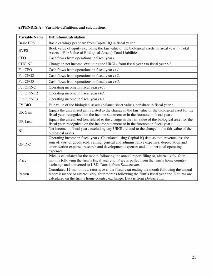
APPENDIX A – Variable definitions and calculations.

Variable Name Definition/Calculation

Basic EPS Basic earnings per share from Capital IQ in fiscal year t.

BVPS Book value of equity excluding the fair value of the biological assets in fiscal year t. (Total Assets – Fair Value of Biological Assets)-Total Liabilities.

CFO Cash flows from operations in fiscal year t.

CHG NI Change in net income, excluding the URGL, from fiscal year t to fiscal year t-1.

Fut CFO Cash flows from operations in fiscal year t+1.

Fut CFO2 Cash flows from operations in fiscal year t+2.

Fut CFO3 Cash flows from operations in fiscal year t+3.

Fut OPINC Operating income in fiscal year t+1.

Fut OPINC2 Operating income in fiscal year t+2.

Fut OPINC3 Operating income in fiscal year t+3.

FV BIO Fair value of the biological assets (balance sheet value), per share in fiscal year t.

UR Gain Equals the unrealized gain related to the change in the fair value of the biological asset for the fiscal year, recognized on the income statement or in the footnote in fiscal year t.

UR Loss Equals the unrealized loss related to the change in the fair value of the biological asset for the fiscal year, recognized on the income statement or in the footnote in fiscal year t.

NI Net income in fiscal year t excluding any URGL related to the change in the fair value of the biological assets.

OP INC

Operating income in fiscal year t. Calculated using Capital IQ data as total revenue less the sum of: cost of goods sold; selling, general and administrative expenses; depreciation and amortization expense; research and development expense; and all other total operating expenses.

Price Price is calculated for the month following the annual report filing or, alternatively, four months following the firm’s fiscal year end. Price is pulled from the firm’s home country exchange and converted to USD. Data is from Datastream.

Return Cumulated 12-month, raw returns over the fiscal year ending the month following the annual report issuance or alternatively, four months following the firm’s fiscal year end. Returns are calculated on the firm’s home country exchange. Data is from Datastream.

26

Table 1 Descriptive sample statistics. Panel A reports the sample composition of the consistent and inconsistent samples by asset value realization and measurement. Cells highlighted in blue comprise firm-year observations classified in the consistent sample, while cells highlighted in yellow comprise firm-year observations classified in the inconsistent sample. Panel B presents the composition of the sample by fiscal year. Panel C presents the composition of the sample by country. PANEL A: Sample composition of consistent and inconsistent firm-year observations by biological asset

value realization and measurement.

Value Realization

In-Exchange In-Use

In-Use and

In-Exchange TOTAL

Measurement

HC 86

(6%) 300

(22%) -

386 (28%)

FV 221

(16%) 543

(40%) 117

(9%) 881

(64%)

HC & FV - - 101

(7%) 101 (7%)

TOTAL

307 (22%)

843 (62%)

218 (16%)

1368 (100%)

PANEL B: Sample composition, in firm-year observations, by fiscal year.

FYEAR Observations % of Total

1999 1 0.07%

2000 5 0.37%

2001 14 1.02%

2002 24 1.75%

2003 42 3.07%

2004 68 4.97%

2005 90 6.58%

2006 126 9.21%

2007 150 10.96%

2008 195 14.25%

2009 217 15.86%

2010 221 16.15%

2011 215 15.72%

Total 1,368 100%

27

Table 1 - Continued Descriptive sample statistics

PANEL C: Sample composition of firms by country of origin.

Country Firms % of Total Country Firms % of Total

Australia 25 10.12% Netherlands 1 0.40%

Brazil 13 5.26% New Zealand 10 4.05%

Canada 9 3.64% Norway 9 3.64%

Channel Islands 2 0.81% Pakistan 1 0.40%

Chile 6 2.43% Papua New Guinea 1 0.40%

China 8 3.24% Peru 3 1.21%

Denmark 3 1.21% Philippines 6 2.43%

Finland 4 1.62% Portugal 3 1.21%

Greece 2 0.81% Singapore 12 4.86%

Hong Kong 17 6.88% South Africa 13 5.26%

Indonesia 1 0.40% Spain 1 0.40%

Ireland 1 0.40% Sri Lanka 9 3.64%

Italy 1 0.40% Sweden 3 1.21%

Jamaica 1 0.40% Switzerland 2 0.81%

Latvia 3 1.21% Thailand 1 0.40%

Lithuania 1 0.40% Turkey 1 0.40%

Luxembourg 2 0.81% Ukraine 5 2.02%

Malaysia 50 20.24% United Kingdom 10 4.05%

Mauritius 2 0.81% Uruguay 1 0.40%

Mexico 1 0.40% Zambia 1 0.40%

Mozambique 1 0.40% Zimbabwe 1 0.40%

TOTAL FIRMS 247 100.00%

28

Table 2 – Panel A Descriptive statistics for the price and return sample. The tables below report the descriptive statistics for the sample used in the value relevance regressions of stock price and returns. The descriptive statistics are reported for the full sample first, then for the consistent sample, and finally for the inconsistent sample. Results from t-statistic tests of difference in means and medians are reported in the consistent sample descriptive statistics. The sample spearman correlation matrix follows the descriptive statistics tables. *** represents significance at the 1% level, ** represents significance at the 5% level, and * represents significance at the 10% level.

Full Sample

Variable Obs Mean Median Std. Dev. Min Max

PRICE 1356 6.57 0.82 35.65 0.00 745.64

BVPS 1356 3.96 0.63 21.82 -3.94 462.16

BASIC EPS 1356 0.13 0.04 2.20 -20.91 44.55

FV BIOPS 1356 0.88 0.07 2.72 -1.26 28.55

UR LOSS PS 1356 -0.02 0.00 0.16 -4.61 0.00

UR GAIN PS 1356 0.10 0.00 0.50 0.00 8.42

RETURN 1136 0.20 0.10 0.91 -0.98 21.98

NI 1136 713.39 205.40 2258.69 0.00 19260.94

CHG NI 1136 -50.12 11.67 2441.50 0.00 36766.23

UR LOSS RET 1136 -36.13 0.00 305.88 -7064.69 0.00

UR GAIN RET 1136 255.39 0.00 1282.35 0.00 18999.32

Consistent Sample

Variable Obs Mean Median Std. Dev. Min Max

PRICE 609 3.28*** 0.70*** 6.38 0.00 37.68

BVPS 609 2.75* 0.58 6.89 -3.94 46.58

BASIC EPS 609 0.14 0.04 1.10 -10.42 10.06

FV BIOPS 609 0.33*** 0*** 1.04 -0.79 12.54

UR LOSS PS 609 0.01 0*** 0.10 0.00 1.89

UR GAIN PS 609 0.07** 0*** 0.43 0.00 5.46

RETURN 512 0.21 0.13 0.58 -0.85 3.58

NI 512 438.39*** 221.27 1637.83 -8954.22 12424.80

CHG NI 512 62.71 31.07** 2307.01 0.00 36766.23

UR LOSS RET 512 -12.21 0*** 67.34 -778.47 0.00

UR GAIN RET 512 111.11*** 0*** 605.30 -3.38 9532.52

29

Table 2 – Panel A Continued Descriptive statistics for the price and return sample.

Inconsistent Sample

Variable Obs Mean Median Std. Dev. Min Max

PRICE 747 9.25 1.06 47.54 0.00 745.64

BVPS 747 4.94 0.71 28.70 -3.71 462.16

BASIC EPS 747 0.12 0.05 2.79 -20.91 44.55

FV BIOPS 747 1.32 0.17 3.49 -1.26 28.55

UR LOSS PS 747 0.02 0.00 0.19 0.00 4.61

UR GAIN PS 747 0.13 0.00 0.55 0.00 8.42

RETURN 624 0.19 0.08 1.12 -0.98 21.98

NI 624 939.03 186.09 2642.15 0.00 19260.94

CHG NI 624 -142.70 0.70 2544.64 0.00 27600.09

UR LOSS RET 624 -55.77 0.00 407.29 -7064.69 0.00

UR GAIN RET 624 373.77 10.62 1632.23 -4482.68 18999.32

Spearman correlations.

PRICE BVPS BASIC EPS FV BIOPS

UR LOSS

UR GAIN

RETURN NI CHG NI CONSISTENT

PRICE 1.00

BVPS 0.81 1.00

BASIC EPS 0.59 0.54 1.00

FV BIOPS 0.56 0.42 0.26 1.00

UR LOSS PS 0.09 0.09 0.09 0.24 1.00

UR GAIN PS 0.38 0.22 0.10 0.55 -0.37 1.00

RETURN -0.05 0.03 0.02 -0.06 0.00 -0.13 1.00

NI 0.44 0.39 0.80 0.15 0.04 0.08 0.02 1.00

CHG NI 0.05 0.04 0.36 -0.10 0.04 -0.17 -0.09 0.43 1.00

CONSISTENT -0.13 -0.03 -0.04 -0.43 -0.11 -0.30 0.08 0.02 0.06 1.00

30

Table 2 – Panel B Descriptive statistics for operating cash flows and operating income sample. The tables below report the descriptive statistics for the sample used in the mechanical forecasting models of operating cash flows and operating income. The descriptive statistics are reported for the full sample first, then for the consistent sample, and finally for the inconsistent sample. Results from t-statistic tests of difference in means and medians are reported in the consistent sample descriptive statistics. The sample spearman correlation matrix follows the descriptive statistics tables. *** represents significance at the 1% level, ** represents significance at the 5% level, and * represents significance at the 10% level.

Full Sample

Variable N Mean Median Std. Dev. Min Max

FUT OP 1368 -0.067 -0.040 0.198 -3.005 0.973

FUT OP2 1132 -0.074 -0.040 0.227 -2.126 0.889

FUT OP3 897 -0.080 -0.050 0.255 -2.384 1.023

OP INC 1368 -0.063 -0.040 0.170 -2.406 0.558

LAG OP INC 1368 -0.061 -0.030 0.197 -4.761 0.306

UR LOSS 1368 -0.004 0.000 0.027 -0.720 0.000

UR GAIN 1368 0.019 0.000 0.057 0.000 0.787

FUT CFO 1368 0.061 0.060 0.123 -1.104 0.852

FUT CFO2 1132 0.073 0.070 0.148 -1.026 1.485

FUT CFO3 897 0.088 0.080 0.159 -0.795 1.244

CFO 1368 0.052 0.060 0.105 -0.893 0.722

NI 1368 0.040 0.050 0.128 -1.243 0.601

Consistent Sample

Variable N Mean Median Std. Dev. Min Max

FUT OP 622 -0.073 -0.020*** 0.233 -3.005 0.973

FUT OP2 515 -0.088* -0.030*** 0.268 -2.126 0.889

FUT OP3 409 -0.106*** -0.040** 0.302 -2.384 0.865

OP INC 622 -0.067 -0.020*** 0.198 -2.406 0.448

LAG OP INC 622 -0.066 -0.020*** 0.256 -4.761 0.243

UR LOSS 622 -0.003 0.000*** 0.031 -0.720 0.000

UR GAIN 622 0.016** 0.000*** 0.055 0.000 0.442

FUT CFO 622 0.065 0.070* 0.135 -1.104 0.547

FUT CFO2 515 0.078 0.08 0.167 -0.902 1.485

FUT CFO3 409 0.091 0.08 0.172 -0.795 1.092

CFO 622 0.053 0.06 0.121 -0.893 0.387

NI 622 0.039 0.05 0.132 -1.049 0.578

31

Table 2 – Panel B Continued Descriptive statistics for operating cash flows and operating income sample.

Inconsistent Sample

Variable N Mean Median Std. Dev. Min Max

FUT OP 746 -0.062 -0.05 0.163 -1.708 0.624

FUT OP2 617 -0.062 -0.05 0.186 -1.949 0.648

FUT OP3 488 -0.058 -0.06 0.205 -1.498 1.023

OP INC 746 -0.059 -0.05 0.142 -1.015 0.558

LAG OP INC 746 -0.057 -0.04 0.128 -0.860 0.306

UR LOSS 746 -0.004 0 0.022 -0.315 0.000

UR GAIN 746 0.023 0 0.058 0.000 0.787

FUT CFO 746 0.058 0.06 0.112 -0.813 0.852

FUT CFO2 617 0.068 0.07 0.131 -1.026 0.700

FUT CFO3 488 0.086 0.07 0.147 -0.789 1.244

CFO 746 0.052 0.06 0.090 -0.483 0.722

NI 746 0.040 0.04 0.124 -1.243 0.601

32

Table 2 – Panel B Continued Descriptive statistics for operating cash flows and operating income sample.

Spearman Correlations

FUT OP FUT OP2 FUT OP3 OP INC LAG OP INC FUT CFO FUT CFO2 FUT

CFO3 CFO NI

UR LOSS

UR GAIN

CONSISTENT

FUT OP 1.00

FUT OP2 0.82 1.00

FUT OP3 0.73 0.82 1.00

OP INC 0.81 0.71 0.68 1.00

LAG OP INC 0.68 0.64 0.61 0.80 1.00

FUT CFO 0.38 0.32 0.25 0.30 0.23 1.00

FUT CFO2 0.35 0.42 0.34 0.31 0.26 0.54 1.00

FUT CFO3 0.33 0.36 0.42 0.32 0.26 0.44 0.56 1.00

CFO 0.31 0.26 0.24 0.35 0.26 0.50 0.43 0.45 1.00

NI 0.40 0.32 0.30 0.52 0.40 0.40 0.36 0.38 0.54 1.00

UR LOSS 0.01 0.01 0.04 0.03 0.05 0.01 0.08 0.03 0.00 0.13 1.00

UR GAIN -0.03 -0.05 -0.04 -0.08 -0.04 -0.05 -0.04 -0.01 -0.02 0.20 0.34 1.00

CONSISTENT 0.03 0.03 0.01 0.03 0.03 0.05 0.05 0.03 0.02 0.02 0.10 -0.28 1.00

33

Table 3 Price and Return Results Table 3 reports the results from the stock price and return estimations over the full sample (FULL), the consistent sample (CON), and the inconsistent sample (INCON). Robust t-statistics, clustered by firm and year, are reported in parentheses below coefficient estimates. Coefficient significance is determined by a two-tailed test. The standard deviation from the bootstrap estimation of the R-squareds and their associated t-statistics, calculated using unequal variances and samples, are reported below the table. Price variables are per share. Return variables are scaled by the log of beginning period market value of equity and have been multiplied by 1,000 for ease of interpretation. See Appendix A for variable definitions. *** represents significance at the 1% level, ** represents significance at the 5% level, and * represents significance at the 10% level.

(1) (2) (3) (4) (5) (6)

FULL CON INCON

FULL CON INCON

VARIABLES Expectations Price Price Price Return Return Return

BVPS + 1.06*** 0.60*** 1.05***

(10.13) (7.97) (8.63)

Basic EPS + 0.79* 1.25* 0.61

(1.95) (1.91) (1.32)

FV BIOPS + 2.08 1.68*** 2.38

(1.27) (3.95) (1.26)

UR LOSS ? 30.31* -7.04*** 40.13**

(1.74) (-2.59) (2.29)

UR GAIN ? -0.67 0.98 -2.70

(-0.24) (1.11) (-0.60)

NI +

-0.00 -0.00 -0.00

(-0.67) (-0.47) (-1.20)

CHG NI +

-0.00 -0.00 -0.00

(-1.31) (-1.29) (-0.90)

UR LOSS ?

-0.00* -0.00 -0.00*

(-1.94) (-1.19) (-1.73)

UR GAIN ?

-0.00** -0.00** -0.00

(-2.19) (-1.99) (-1.43)

Intercept

0.03 0.92*** 0.47

211.73** 229.67** 206.85**

(0.09) (4.58) (0.91)

(2.16) (2.30) (2.06)

Observations

1,356 609 747

1,136 512 624

R-squared 0.66 0.74 0.67 0.00 0.02 0.00

Bootstrapped Standard Deviation 0.037 0.178

0.011 0.007

T-statistic of Difference

4.18***

2.34**

34

Table 4 Operating Cash Flows Results Table 4 reports the results from the mechanical forecasting model for future cash flows from operations. The results are presented for estimations over the full sample (FULL), the consistent sample (CON), and the inconsistent sample (INCON). Robust t-statistics, clustered by firm, are reported in parentheses below coefficient estimates. Country fixed effects are included in all estimations. Coefficient significance is determined by a two-tailed test. The standard deviation from the bootstrap estimation of the R-squareds and their associated t-statistics, calculated using unequal variances and samples, are reported below the table. All variables are scaled by average total assets. See Appendix A for variable definitions. *** represents significance at the 1% level, ** represents significance at the 5% level, and * represents significance at the 10% level.

(1) (2) (3) (4) (5) (6) (7) (8) (9)

FULL CON INCON

FULL CON INCON

FULL CON INCON

VARIABLES Expectations Fut CFO Fut CFO Fut CFO

Fut CFO2 Fut CFO2 Fut CFO2

Fut CFO3 Fut CFO3 Fut CFO3

CFO + 0.429*** 0.438*** 0.352***

0.452*** 0.372*** 0.398***

0.473*** 0.443*** 0.409***

(5.442) (4.397) (2.861)

(6.528) (3.090) (4.023)

(4.897) (3.655) (3.834)

NI + 0.263*** 0.270*** 0.264***

0.236*** 0.305* 0.196**

0.288*** 0.223** 0.349**

(4.582) (2.863) (3.791)

(2.957) (1.910) (2.275)

(2.845) (2.306) (2.126)

UR LOSS ? -0.319* -0.526*** 0.106

-0.254* -0.435*** 0.066

0.123 -0.009 0.284

(-1.960) (-6.165) (0.807)

(-1.652) (-3.352) (0.326)

(1.052) (-0.092) (1.069)

UR GAIN ? -0.238*** -0.357 -0.177***

-0.262** -1.177** -0.112

-0.319*** -1.414*** -0.227*

(-3.969) (-1.606) (-3.414)

(-2.409) (-2.537) (-1.062)

(-3.007) (-4.576) (-1.757)

Intercept

0.034*** 0.039*** 0.033***

0.044*** 0.065*** 0.040***

0.055*** 0.078*** 0.051***

(7.876) (7.258) (4.658)

(8.643) (6.663) (4.453)

(7.846) (8.247) (5.280)

Observations

1,368 622 746

1,132 515 617

897 409 488

R-squared 0.436 0.529 0.368 0.324 0.427 0.255 0.337 0.456 0.299

Country Fixed Effects Y Y Y

Y Y Y

Y Y Y

Bootstrapped Standard Deviation 0.094 0.053

0.085 0.047

0.075 0.072

T-statistic of Difference

10.78***

11.07***

8.64***

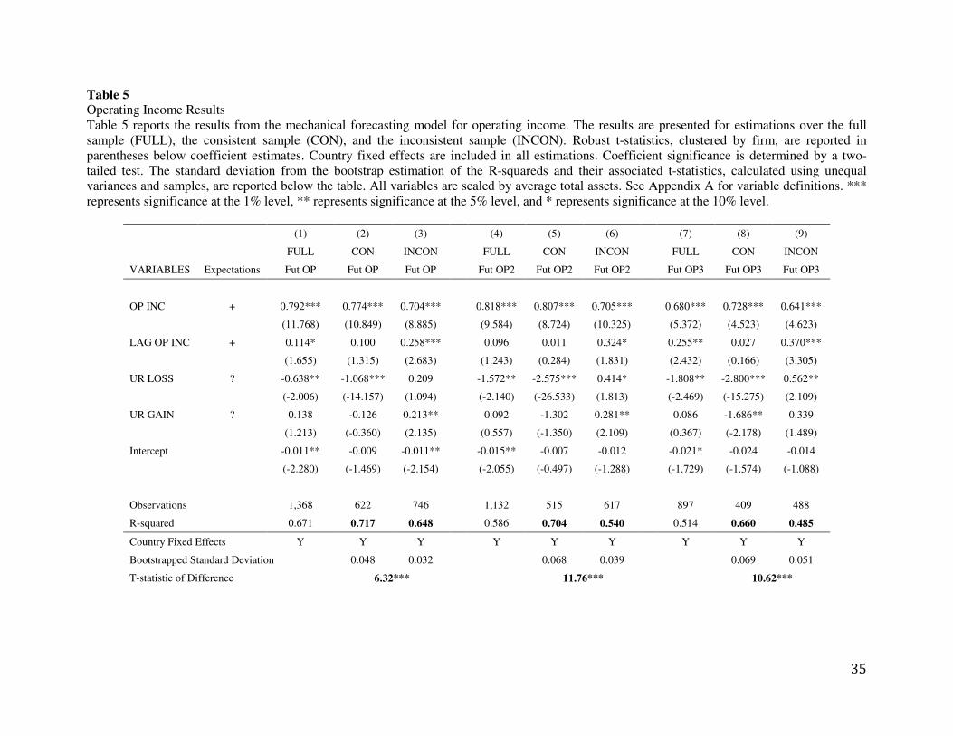
35

Table 5 Operating Income Results Table 5 reports the results from the mechanical forecasting model for operating income. The results are presented for estimations over the full sample (FULL), the consistent sample (CON), and the inconsistent sample (INCON). Robust t-statistics, clustered by firm, are reported in parentheses below coefficient estimates. Country fixed effects are included in all estimations. Coefficient significance is determined by a two-tailed test. The standard deviation from the bootstrap estimation of the R-squareds and their associated t-statistics, calculated using unequal variances and samples, are reported below the table. All variables are scaled by average total assets. See Appendix A for variable definitions. *** represents significance at the 1% level, ** represents significance at the 5% level, and * represents significance at the 10% level.

(1) (2) (3) (4) (5) (6) (7) (8) (9)

FULL CON INCON

FULL CON INCON

FULL CON INCON

VARIABLES Expectations Fut OP Fut OP Fut OP

Fut OP2 Fut OP2 Fut OP2

Fut OP3 Fut OP3 Fut OP3

OP INC + 0.792*** 0.774*** 0.704***

0.818*** 0.807*** 0.705***

0.680*** 0.728*** 0.641***

(11.768) (10.849) (8.885)

(9.584) (8.724) (10.325)

(5.372) (4.523) (4.623)

LAG OP INC + 0.114* 0.100 0.258***

0.096 0.011 0.324*

0.255** 0.027 0.370***

(1.655) (1.315) (2.683)

(1.243) (0.284) (1.831)

(2.432) (0.166) (3.305)

UR LOSS ? -0.638** -1.068*** 0.209

-1.572** -2.575*** 0.414*

-1.808** -2.800*** 0.562**

(-2.006) (-14.157) (1.094)

(-2.140) (-26.533) (1.813)

(-2.469) (-15.275) (2.109)

UR GAIN ? 0.138 -0.126 0.213**

0.092 -1.302 0.281**

0.086 -1.686** 0.339

(1.213) (-0.360) (2.135)

(0.557) (-1.350) (2.109)

(0.367) (-2.178) (1.489)

Intercept

-0.011** -0.009 -0.011**

-0.015** -0.007 -0.012

-0.021* -0.024 -0.014

(-2.280) (-1.469) (-2.154)

(-2.055) (-0.497) (-1.288)

(-1.729) (-1.574) (-1.088)

Observations

1,368 622 746

1,132 515 617

897 409 488

R-squared 0.671 0.717 0.648 0.586 0.704 0.540 0.514 0.660 0.485

Country Fixed Effects Y Y Y

Y Y Y

Y Y Y

Bootstrapped Standard Deviation 0.048 0.032

0.068 0.039

0.069 0.051

T-statistic of Difference

6.32***

11.76***

10.62***