Decision Tree Induction

Decision Tree Induction

Many Algorithms:– Hunt’s Algorithm (one of the earliest)– Hunt s Algorithm (one of the earliest)– CART

ID3 C4 5– ID3, C4.5– SLIQ,SPRINT

© Tan,Steinbach, Kumar Introduction to Data Mining 4/18/2004 ‹#›

General Structure of Hunt’s Algorithm

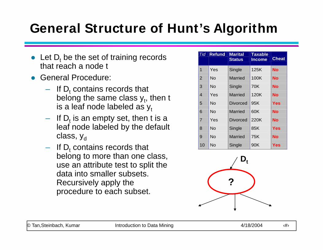
Let Dt be the set of training records that reach a node tGeneral Procedure:

Tid Refund Marital Status

Taxable Income Cheat

1 Yes Single 125K No

2 No Married 100K NoGeneral Procedure:– If Dt contains records that

belong the same class yt, then t is a leaf node labeled as yt

2 No Married 100K No

3 No Single 70K No

4 Yes Married 120K No

5 No Divorced 95K Yes s a ea ode abe ed as yt

– If Dt is an empty set, then t is a leaf node labeled by the default class, yd

6 No Married 60K No

7 Yes Divorced 220K No

8 No Single 85K Yes

9 No Married 75K No

– If Dt contains records that belong to more than one class, use an attribute test to split the data into smaller subsets

10 No Single 90K Yes 10

Dt

data into smaller subsets. Recursively apply the procedure to each subset.

?


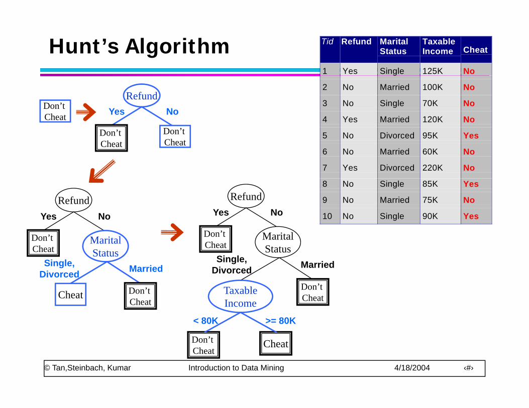
Hunt’s Algorithm Tid Refund MaritalStatus

TaxableIncome Cheat

1 Yes Single 125K No

Don’t Cheat

RefundYes No

g


3 No Single 70K No

4 Yes Married 120K NoDon’t Cheat

Don’t Cheat

5 No Divorced 95K Yes

6 No Married 60K No


RefundYes No

RefundYes No

8 No Single 85K Yes

9 No Married 75K No

10 No Single 90K Yes10

Don’t Cheat

MaritalStatus

Single,Divorced Married

Don’t Cheat

MaritalStatus

Single,Divorced Married

Don’t Cheat

TaxableIncome

< 80K >= 80K

Don’t Cheat

Cheat


CheatDon’t Cheat

Tree Induction

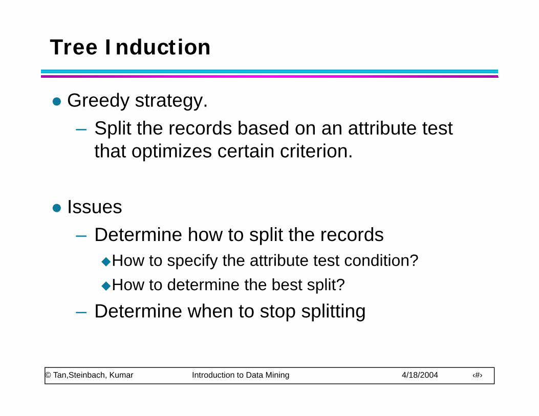
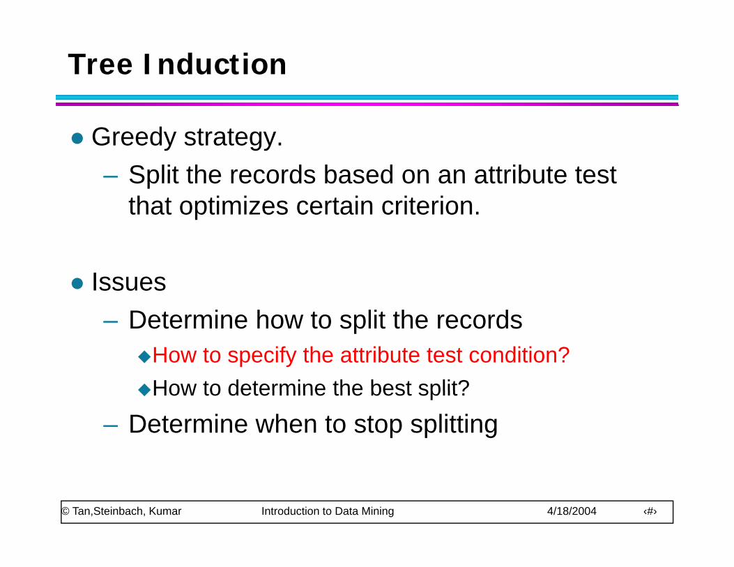
Greedy strategy.– Split the records based on an attribute test– Split the records based on an attribute test

that optimizes certain criterion.

IssuesDetermine how to split the records– Determine how to split the records

How to specify the attribute test condition?How to determine the best split?How to determine the best split?

– Determine when to stop splitting


Tree Induction







How to Specify Test Condition?

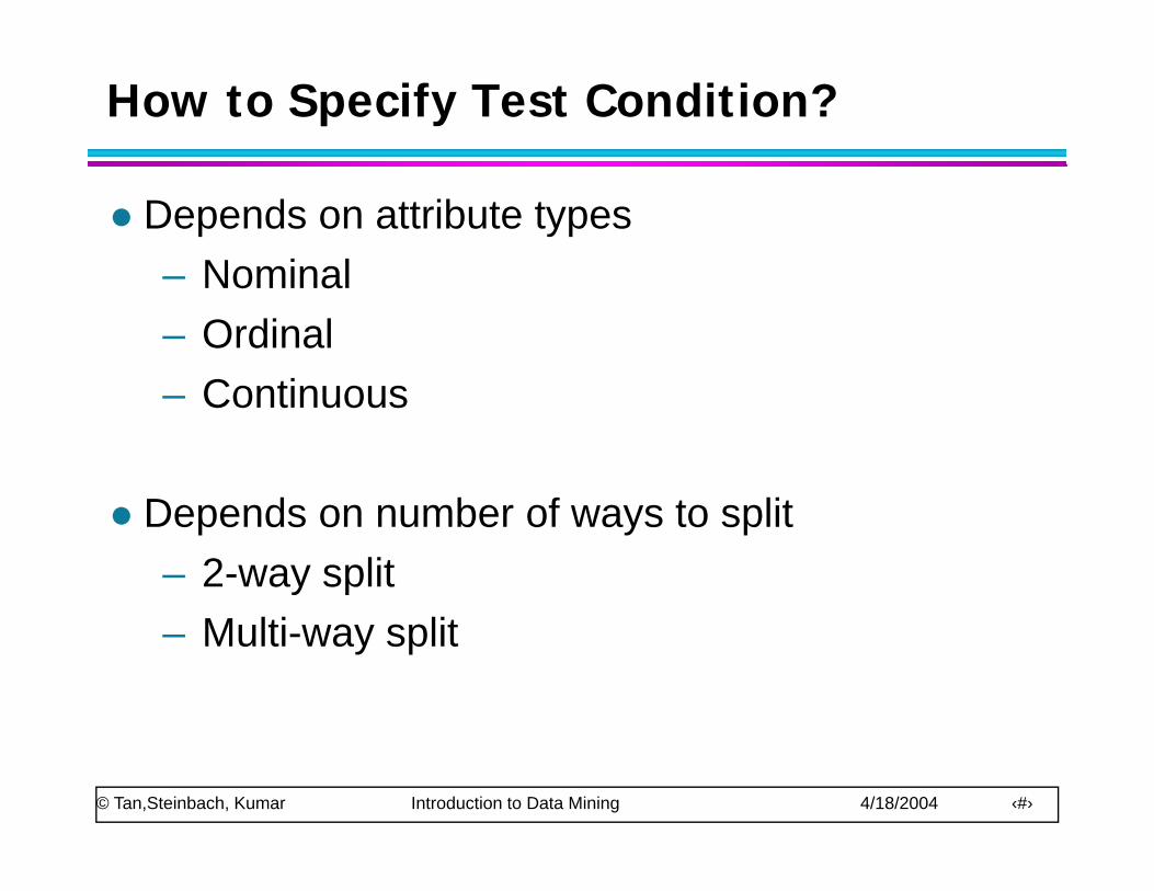
Depends on attribute types– Nominal– Nominal– Ordinal

Continuous– Continuous

D d b f t litDepends on number of ways to split– 2-way split– Multi-way split


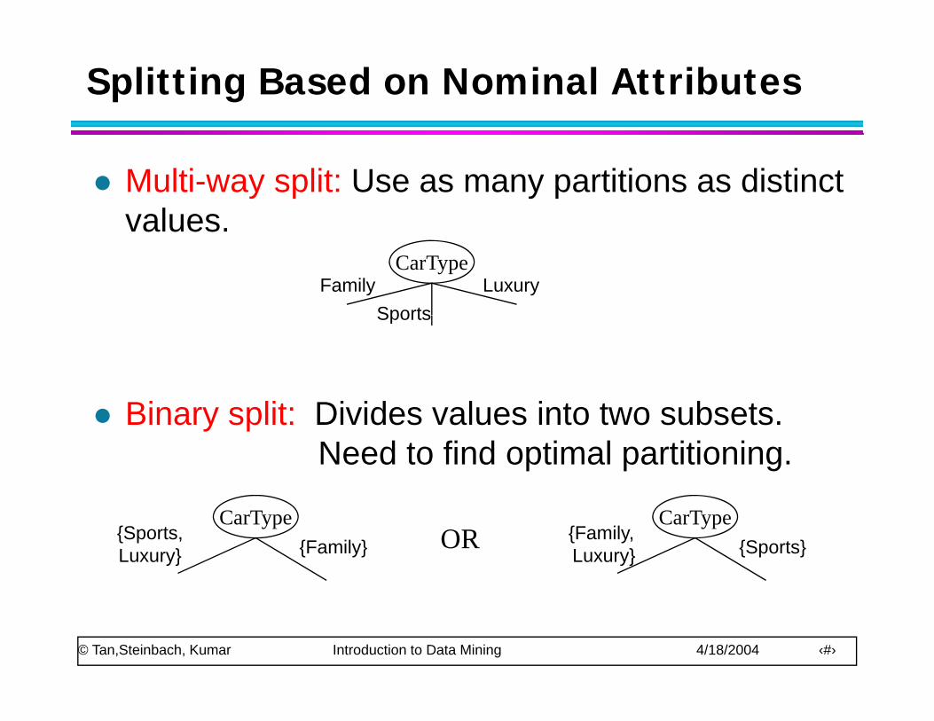
Splitting Based on Nominal Attributes

Multi-way split: Use as many partitions as distinct valuesvalues.

CarTypeFamily

SportsLuxury

Bi lit Di id l i t t b t

Sports

Binary split: Divides values into two subsets. Need to find optimal partitioning.

CarType{Family, Luxury} {Sports}

CarType{Sports, Luxury} {Family} OR


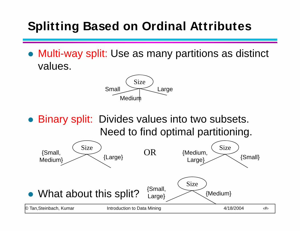
Splitting Based on Ordinal Attributes

Multi-way split: Use as many partitions as distinct values.

SizeSmall

MediumLarge

Binary split: Divides values into two subsets. Need to find optimal partitioningNeed to find optimal partitioning.

Size{Medium,

Large} {Small}Size

{Small, Medium} {Large} OR

Large} { }Medium} { g }

Size{Small


What about this split? {Small, Large} {Medium}

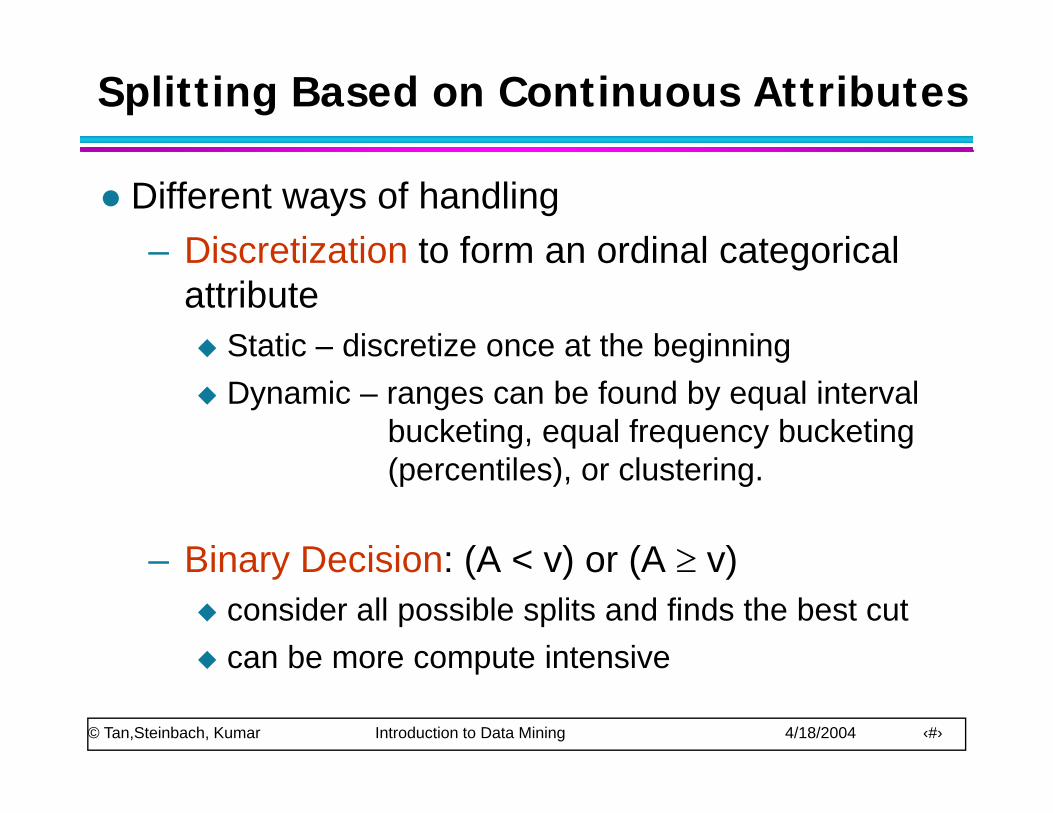
Splitting Based on Continuous Attributes

Different ways of handling– Discretization to form an ordinal categorical– Discretization to form an ordinal categorical

attributeStatic – discretize once at the beginningStatic discretize once at the beginningDynamic – ranges can be found by equal interval

bucketing, equal frequency bucketing( til ) l t i(percentiles), or clustering.

Binary Decision: (A < v) or (A ≥ v)– Binary Decision: (A < v) or (A ≥ v)consider all possible splits and finds the best cutcan be more compute intensive


can be more compute intensive

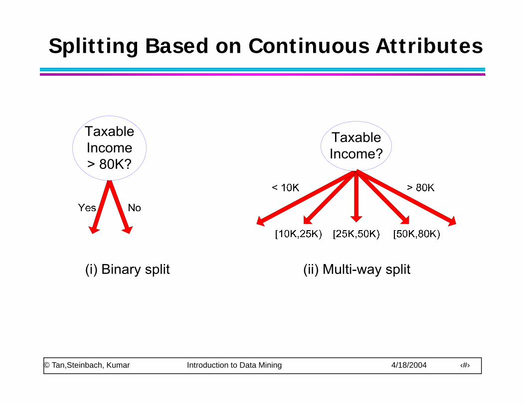
Splitting Based on Continuous Attributes


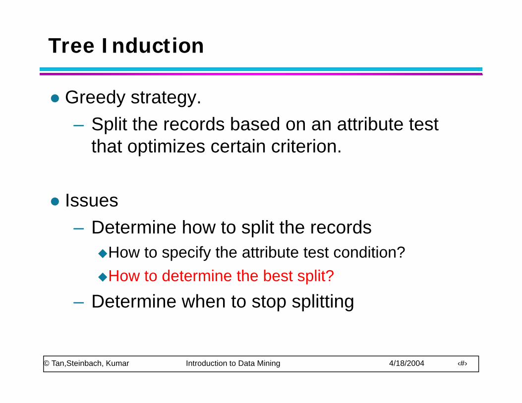
Tree Induction







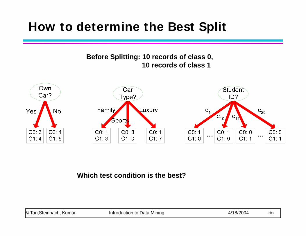
How to determine the Best Split

Before Splitting: 10 records of class 0,10 records of class 1

Which test condition is the best?


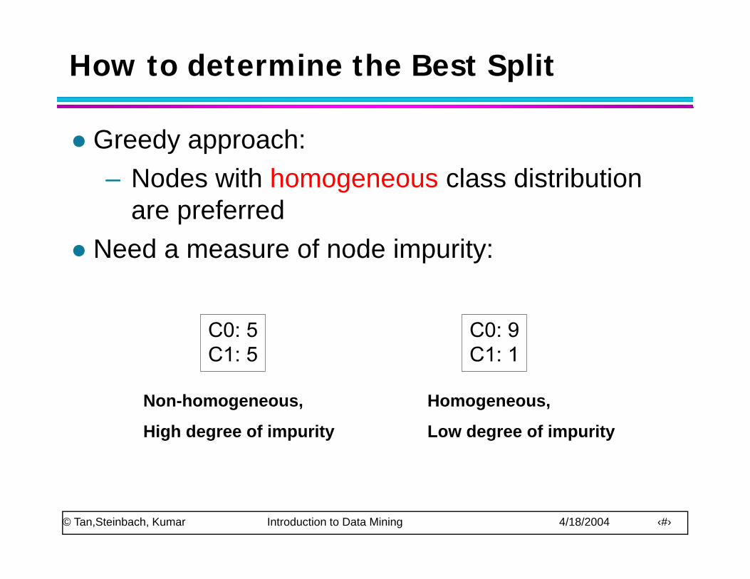
How to determine the Best Split

Greedy approach: – Nodes with homogeneous class distribution– Nodes with homogeneous class distribution

are preferredNeed a measure of node impurity:Need a measure of node impurity:

Non homogeneous HomogeneousNon-homogeneous,

High degree of impurity

Homogeneous,

Low degree of impurity


Measures of Node Impurity

Gini Index

Entropy

Misclassification error


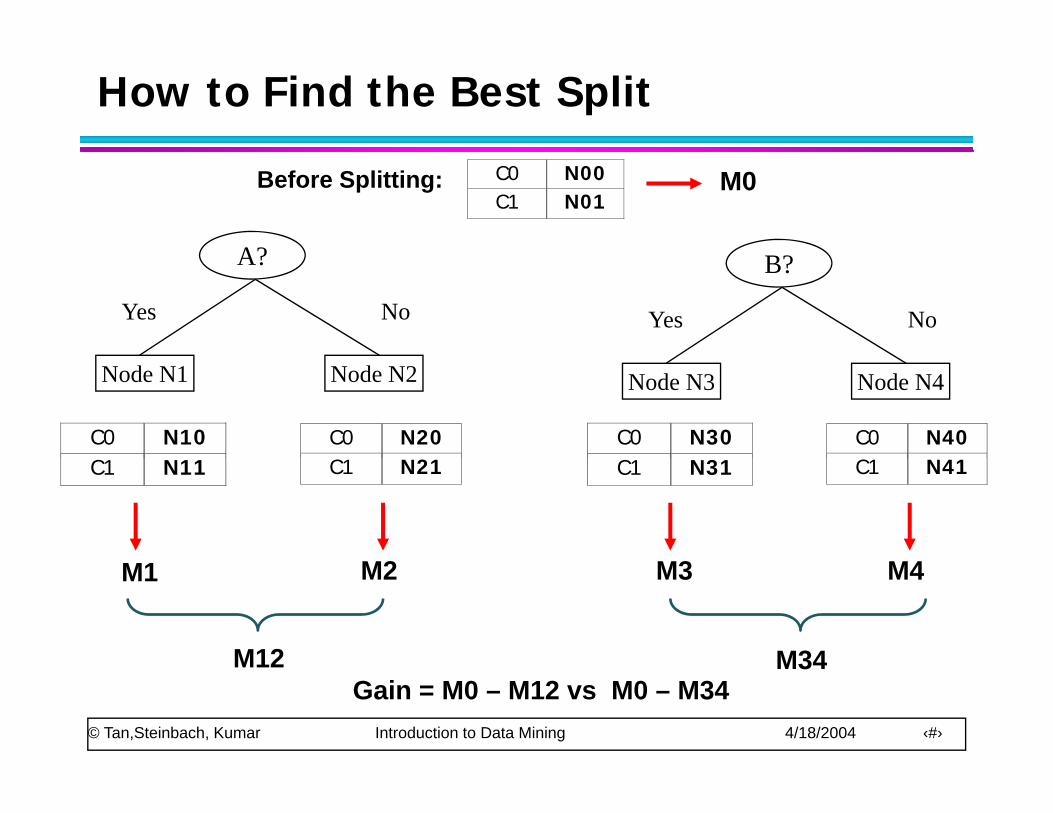
How to Find the Best Split

A?

Before Splitting: C0 N00 C1 N01

M0

B?

Yes No

A?

Yes No

Node N3 Node N4Node N1 Node N2

C0 N10 C0 N20 C0 N30 C0 N40 C1 N11

C1 N21

C1 N31

C1 N41

M2 M3 M4M1 M2 M3 M4

M12 M34


M12 M34Gain = M0 – M12 vs M0 – M34

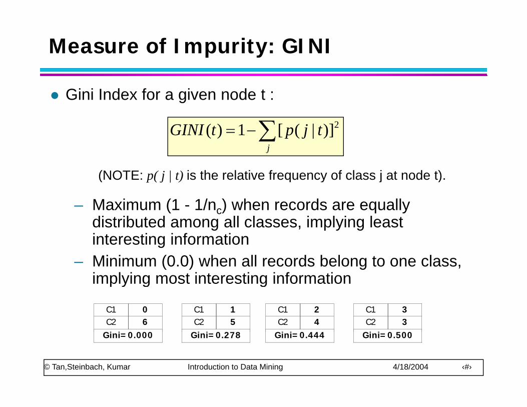
Measure of Impurity: GINI

Gini Index for a given node t :

∑ tjtGINI 2)]|([1)(

(NOTE: p( j | t) is the relative frequency of class j at node t)

∑−=j

tjptGINI 2)]|([1)(

(NOTE: p( j | t) is the relative frequency of class j at node t).

– Maximum (1 - 1/nc) when records are equally distributed among all classes, implying least g , p y ginteresting information

– Minimum (0.0) when all records belong to one class, implying most interesting informationimplying most interesting information

C1 0C2 6

Gi i 0 000

C1 2C2 4

Gi i 0 444

C1 3C2 3

Gi i 0 500

C1 1C2 5

Gi i 0 278


Gini=0.000 Gini=0.444 Gini=0.500Gini=0.278

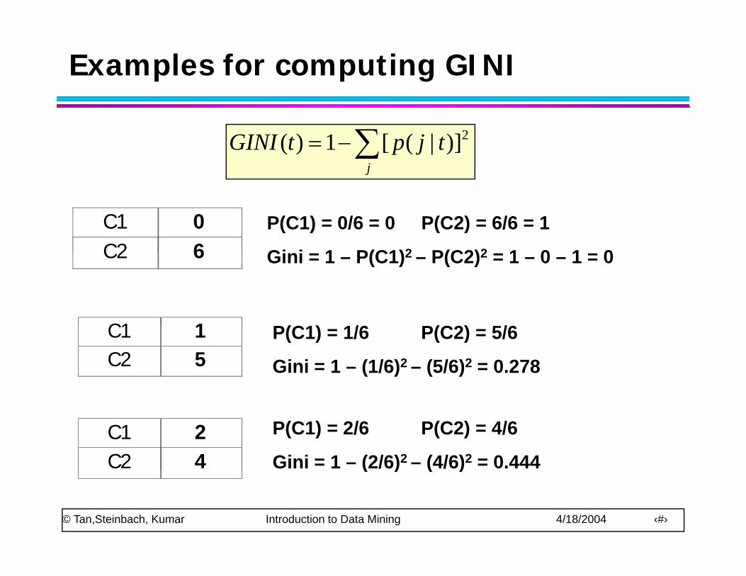
Examples for computing GINI

∑−=j

tjptGINI 2)]|([1)(

C1 0 C2 6

P(C1) = 0/6 = 0 P(C2) = 6/6 = 1

Gi i 1 P(C1)2 P(C2)2 1 0 1 0C2 6

C1 1

Gini = 1 – P(C1)2 – P(C2)2 = 1 – 0 – 1 = 0

C1 1 C2 5

P(C1) = 1/6 P(C2) = 5/6

Gini = 1 – (1/6)2 – (5/6)2 = 0.278

C1 2 C2 4

P(C1) = 2/6 P(C2) = 4/6

Gini = 1 – (2/6)2 – (4/6)2 = 0.444


( ) ( )

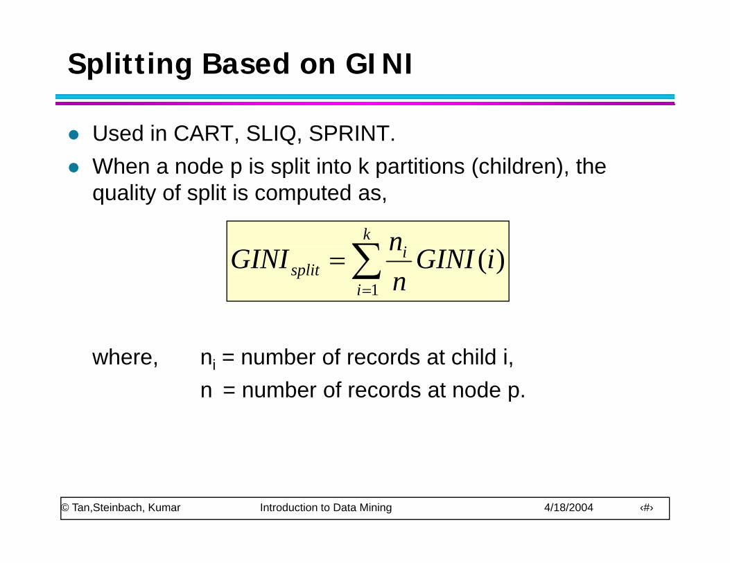
Splitting Based on GINI

Used in CART, SLIQ, SPRINT.When a node p is split into k partitions (children), the p p p ( ),quality of split is computed as,

∑k n∑=

=i

isplit iGINI

nnGINI

1)(

where, ni = number of records at child i,n = number of records at node pn = number of records at node p.


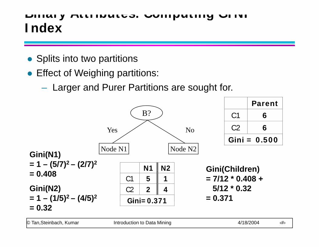
Binary Attributes: Computing GINI Index

Splits into two partitionsEffect of Weighing partitions: g g p– Larger and Purer Partitions are sought for.

ParentB?

Yes No

C1 6

C2 6

Gini = 0 500Node N1 Node N2

Gini = 0.500

N1 N2

Gini(N1) = 1 – (5/7)2 – (2/7)2

Gini(Children)N1 N2C1 5 1 C2 2 4 Gini=0 371

= 0.408

Gini(N2) = 1 – (1/5)2 – (4/5)2

Gini(Children) = 7/12 * 0.408 +

5/12 * 0.32= 0.371


Gini=0.371

( ) ( )= 0.32

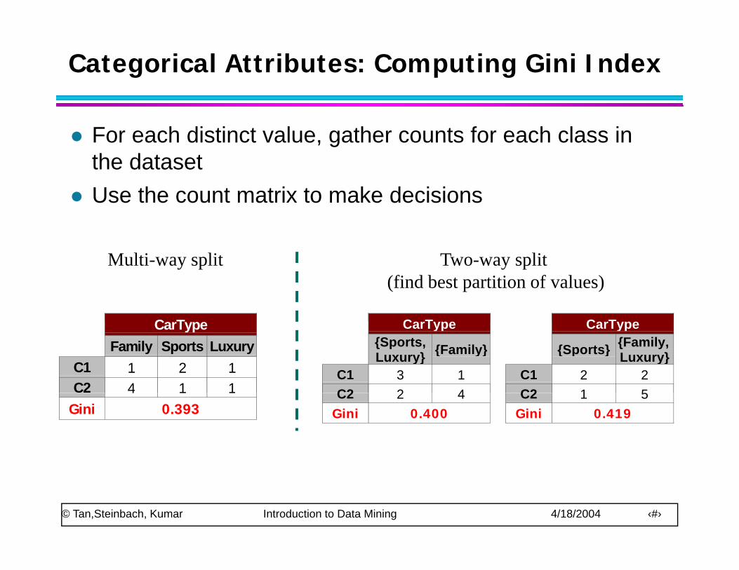
Categorical Attributes: Computing Gini Index

For each distinct value, gather counts for each class in the datasetUse the count matrix to make decisions

C T C TC T

Multi-way split Two-way split (find best partition of values)

CarType{Sports,Luxury} {Family}

C1 3 1C2 2 4

CarType

{Sports} {Family,Luxury}

C1 2 2C2 1 5

CarTypeFamily Sports Luxury

C1 1 2 1C2 4 1 1 C2 2 4

Gini 0.400C2 1 5

Gini 0.419

4 1 1Gini 0.393


Continuous Attributes: Computing Gini Index

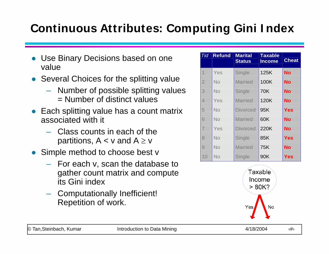
Use Binary Decisions based on one valueSeveral Choices for the splitting value

Tid Refund Marital Status

Taxable Income Cheat

1 Yes Single 125K No Several Choices for the splitting value

– Number of possible splitting values = Number of distinct values

Each splitting value has a count matrix


3 No Single 70K No

4 Yes Married 120K No

5 No Divorced 95K YesEach splitting value has a count matrix associated with it

– Class counts in each of the partitions, A < v and A ≥ v

5 No Divorced 95K Yes

6 No Married 60K No


8 No Single 85K Yes partitions, A v and A ≥ vSimple method to choose best v

– For each v, scan the database to gather count matrix and compute

9 No Married 75K No

10 No Single 90K Yes 10

gather count matrix and compute its Gini index

– Computationally Inefficient! Repetition of work.


Continuous Attributes: Computing Gini Index...

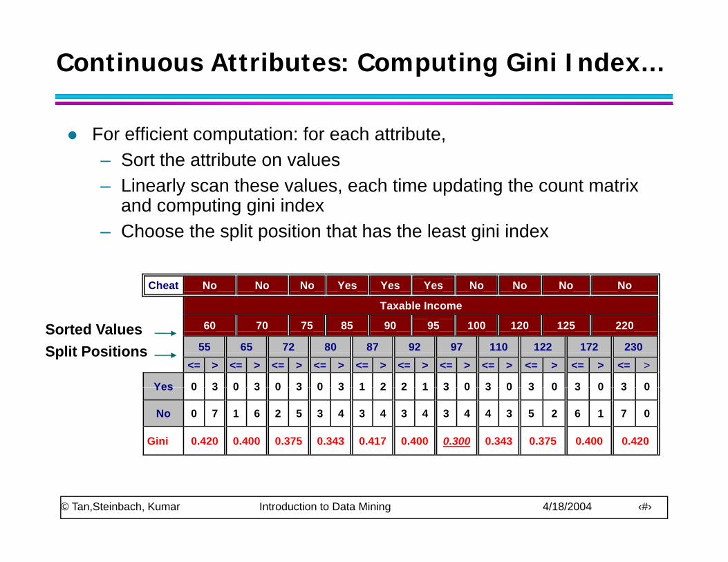
For efficient computation: for each attribute,– Sort the attribute on values– Linearly scan these values, each time updating the count matrix

and computing gini index– Choose the split position that has the least gini index

Cheat No No No Yes Yes Yes No No No No

Taxable Income

60 70 75 85 90 95 100 120 125 220

55 65 72 80 87 92 97 110 122 172 230<= > <= > <= > <= > <= > <= > <= > <= > <= > <= > <= >

Yes 0 3 0 3 0 3 0 3 1 2 2 1 3 0 3 0 3 0 3 0 3 0

Split PositionsSorted Values

Yes 0 3 0 3 0 3 0 3 1 2 2 1 3 0 3 0 3 0 3 0 3 0

No 0 7 1 6 2 5 3 4 3 4 3 4 3 4 4 3 5 2 6 1 7 0

Gini 0.420 0.400 0.375 0.343 0.417 0.400 0.300 0.343 0.375 0.400 0.420


Alternative Splitting Criteria based on INFO

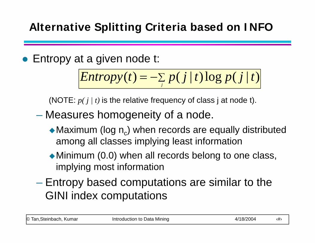
Entropy at a given node t:∑ tjptjptEntropy )|(log)|()(

(NOTE: p( j | t) is the relative frequency of class j at node t).

∑−=j

tjptjptEntropy )|(log)|()(

– Measures homogeneity of a node. Maximum (log nc) when records are equally distributed among all classes implying least informationMinimum (0.0) when all records belong to one class, implying most informationimplying most information

– Entropy based computations are similar to the GINI index computations


GINI index computations

Examples for computing Entropy

∑−=j

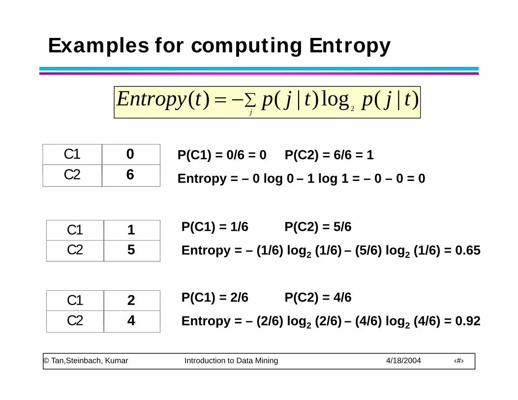
tjptjptEntropy )|(log)|()(2

C1 0 C2 6

P(C1) = 0/6 = 0 P(C2) = 6/6 = 1

E t 0 l 0 1 l 1 0 0 0C2 6

C1 1

Entropy = – 0 log 0 – 1 log 1 = – 0 – 0 = 0

P(C1) = 1/6 P(C2) = 5/6C1 1 C2 5

P(C1) = 1/6 P(C2) = 5/6

Entropy = – (1/6) log2 (1/6) – (5/6) log2 (1/6) = 0.65

C1 2 C2 4

P(C1) = 2/6 P(C2) = 4/6

Entropy = – (2/6) log2 (2/6) – (4/6) log2 (4/6) = 0.92


py ( ) g2 ( ) ( ) g2 ( )

Splitting Based on INFO...

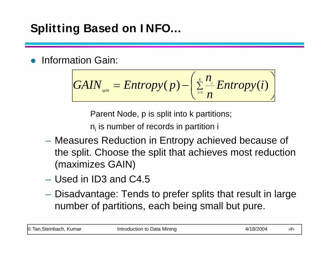
Information Gain:

⎞⎛ k n

P t N d i lit i t k titi

⎟⎠⎞

⎜⎝⎛−= ∑

=

k

i

i

splitiEntropy

nnpEntropyGAIN

1)()(

Parent Node, p is split into k partitions;ni is number of records in partition i

– Measures Reduction in Entropy achieved because ofMeasures Reduction in Entropy achieved because of the split. Choose the split that achieves most reduction (maximizes GAIN)

– Used in ID3 and C4.5– Disadvantage: Tends to prefer splits that result in large

number of partitions each being small but pure


number of partitions, each being small but pure.

Splitting Based on INFO...

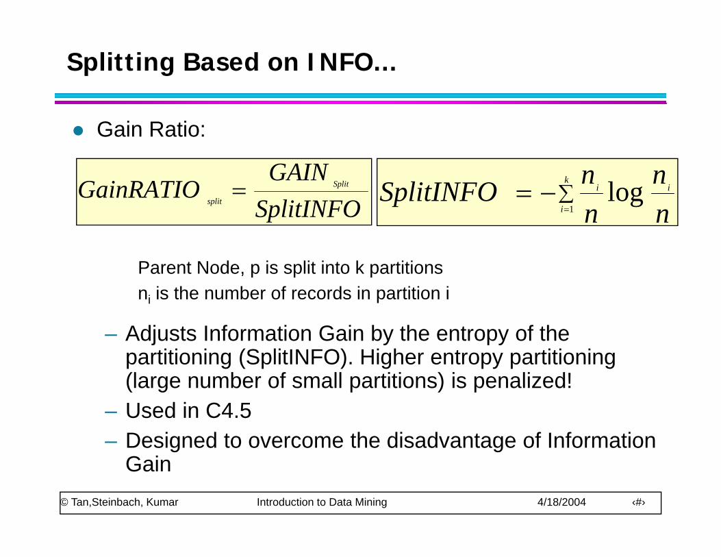
Gain Ratio:

GAIN nnSplitINFO

GAINGainRATIO Split

split= ∑

=−=

k

i

ii

nn

nnSplitINFO

1log

Parent Node, p is split into k partitionsni is the number of records in partition i

– Adjusts Information Gain by the entropy of the partitioning (SplitINFO). Higher entropy partitioning (large number of small partitions) is penalized!(large number of small partitions) is penalized!

– Used in C4.5– Designed to overcome the disadvantage of Information


Gain

Splitting Criteria based on Classification Error

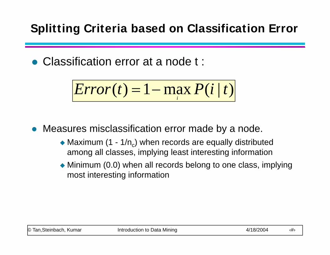
Classification error at a node t :

)|(max1)( tiPtErrori

−=

Measures misclassification error made by a node. Maximum (1 - 1/n ) when records are equally distributedMaximum (1 1/nc) when records are equally distributed among all classes, implying least interesting informationMinimum (0.0) when all records belong to one class, implying most interesting informationmost interesting information


Examples for Computing Error

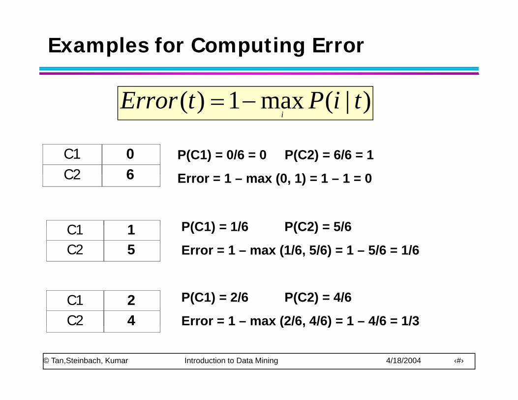
)|(max1)( tiPtErrori

−=

C1 0 C2 6

P(C1) = 0/6 = 0 P(C2) = 6/6 = 1

E 1 (0 1) 1 1 0C2 6

C1 1

Error = 1 – max (0, 1) = 1 – 1 = 0

P(C1) = 1/6 P(C2) = 5/6C1 1 C2 5

P(C1) = 1/6 P(C2) = 5/6

Error = 1 – max (1/6, 5/6) = 1 – 5/6 = 1/6

C1 2 C2 4

P(C1) = 2/6 P(C2) = 4/6

Error = 1 – max (2/6, 4/6) = 1 – 4/6 = 1/3


( , )

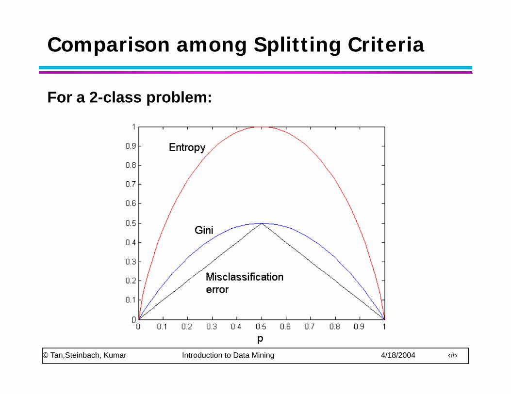
Comparison among Splitting Criteria

For a 2-class problem:


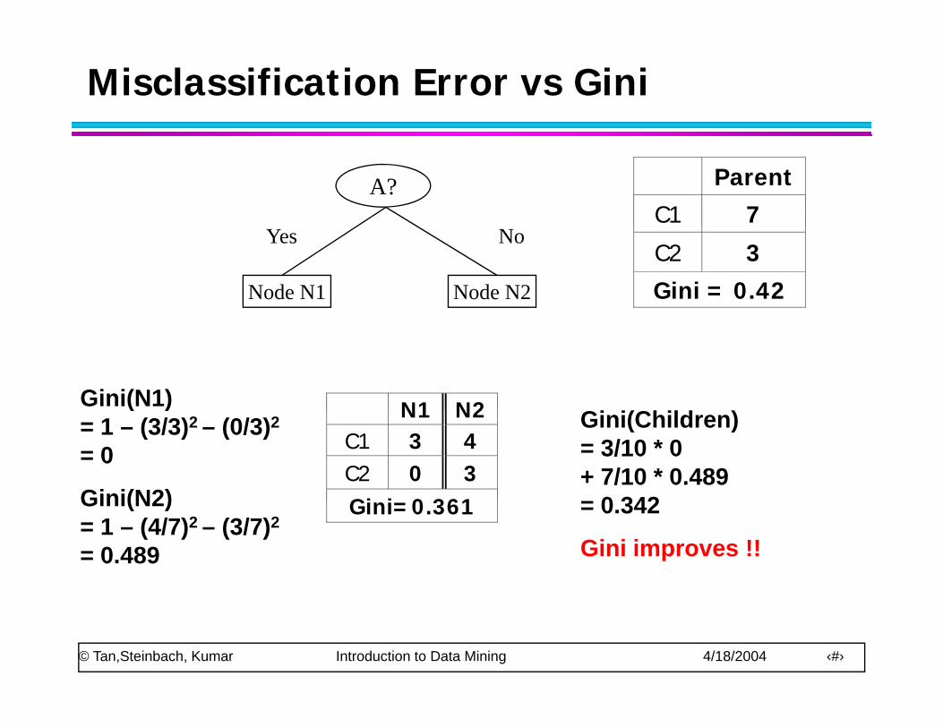
Misclassification Error vs Gini

A? ParentC1 7

Yes No

Node N1 Node N2

C2 3

Gini = 0.42

N1 N2Gini(N1) N1 N2C1 3 4 C2 0 3 Gini 0 361

( )= 1 – (3/3)2 – (0/3)2

= 0

Gini(N2)

Gini(Children) = 3/10 * 0 + 7/10 * 0.489= 0 342Gini=0.361

Gini(N2) = 1 – (4/7)2 – (3/7)2

= 0.489

= 0.342

Gini improves !!


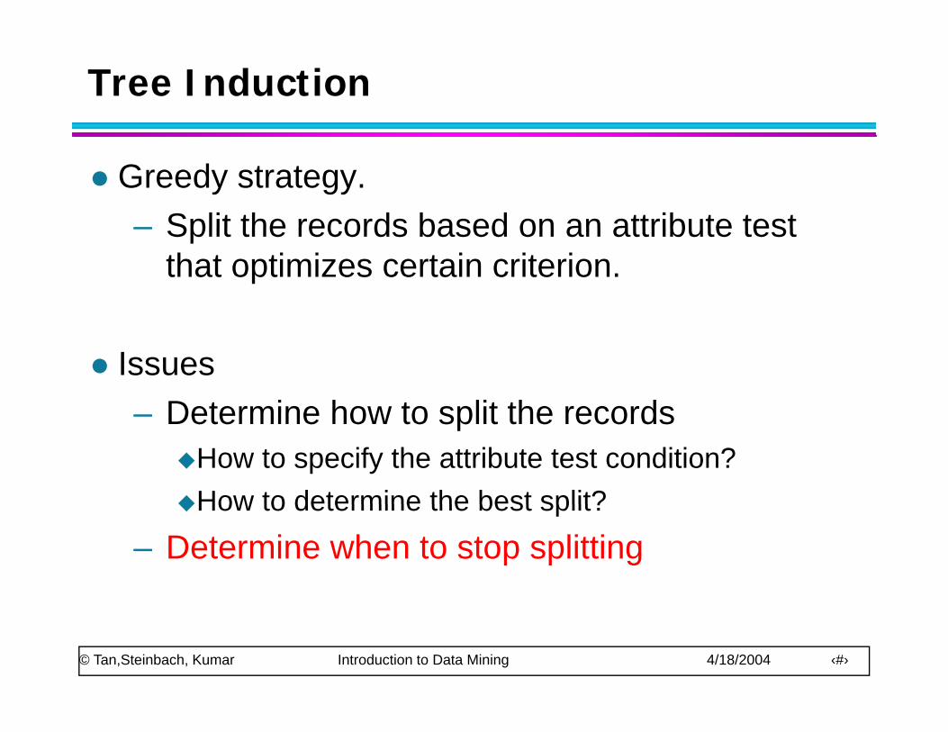
Tree Induction







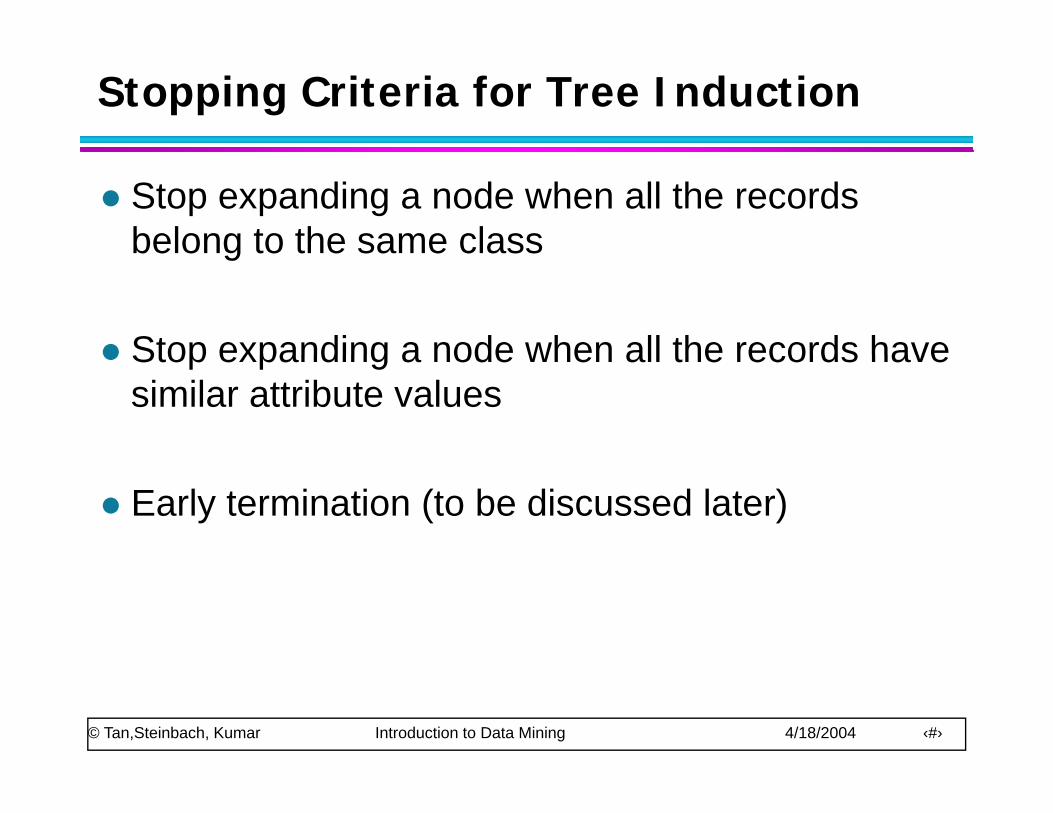
Stopping Criteria for Tree Induction

Stop expanding a node when all the records belong to the same classbelong to the same class

Stop expanding a node when all the records haveStop expanding a node when all the records have similar attribute values

Early termination (to be discussed later)


Decision Tree Based Classification

Advantages:– Inexpensive to construct– Inexpensive to construct– Extremely fast at classifying unknown records

Easy to interpret for small sized trees– Easy to interpret for small-sized trees– Accuracy is comparable to other classification

techniques for many simple data setstechniques for many simple data sets


Example: C4.5

Simple depth-first construction.Uses Information GainUses Information GainSorts Continuous Attributes at each node.Needs entire data to fit in memoryNeeds entire data to fit in memory.Unsuitable for Large Datasets.

N d t f ti– Needs out-of-core sorting.

You can download the software from:http://www.cse.unsw.edu.au/~quinlan/c4.5r8.tar.gz


Practical Issues of Classification

Underfitting and Overfitting

Missing Values

Costs of Classification


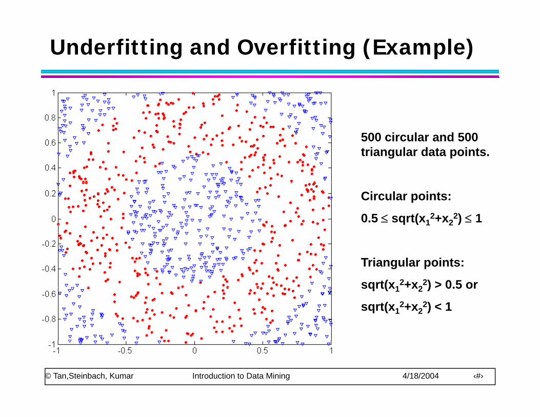
Underfitting and Overfitting (Example)

500 circular and 500 triangular data points.

Circular points:

0.5 ≤ sqrt(x12+x2

2) ≤ 1

Triangular points:

sqrt(x12+x2

2) > 0.5 orsqrt(x1 x2 ) > 0.5 or

sqrt(x12+x2

2) < 1


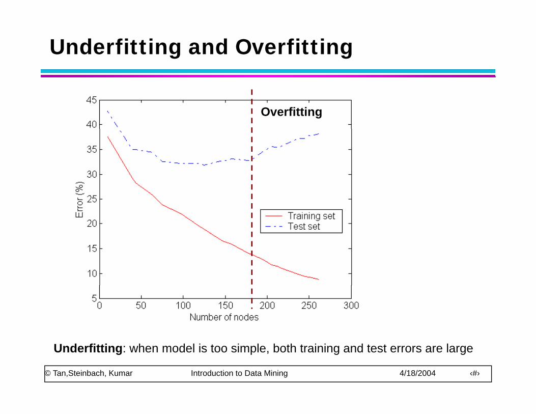
Underfitting and Overfitting

Overfitting


Underfitting: when model is too simple, both training and test errors are large

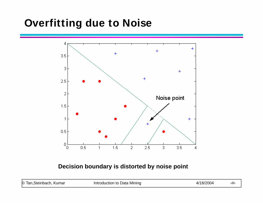
Overfitting due to Noise

Decision boundary is distorted by noise point


Decision boundary is distorted by noise point

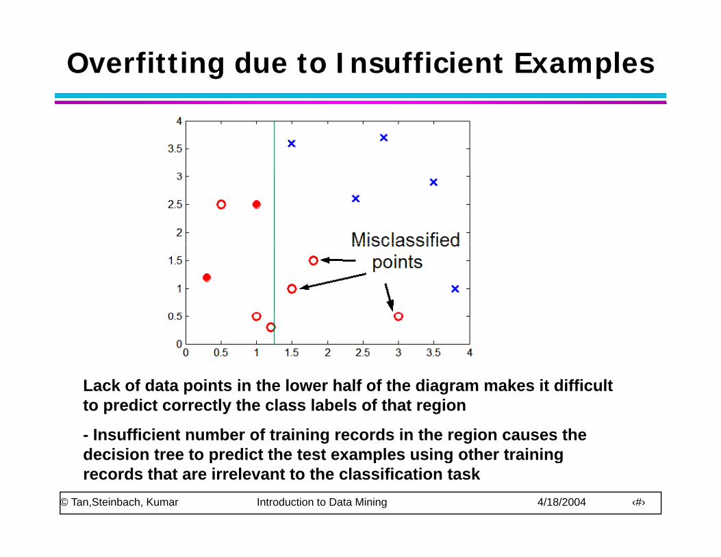
Overfitting due to Insufficient Examples

Lack of data points in the lower half of the diagram makes it difficultLack of data points in the lower half of the diagram makes it difficult to predict correctly the class labels of that region

- Insufficient number of training records in the region causes the decision tree to predict the test examples using other training


decision tree to predict the test examples using other training records that are irrelevant to the classification task

Notes on Overfitting

Overfitting results in decision trees that are more complex than necessarycomplex than necessary

Training error no longer provides a good estimateTraining error no longer provides a good estimate of how well the tree will perform on previously unseen records

Need new ways for estimating errorseed e ays o est at g e o s


Estimating Generalization Errors

Re-substitution errors: error on training (Σ e(t) )Generalization errors: error on testing (Σ e’(t))Methods for estimating generalization errors:– Optimistic approach: e’(t) = e(t)– Pessimistic approach:– Pessimistic approach:

For each leaf node: e’(t) = (e(t)+0.5) Total errors: e’(T) = e(T) + N × 0.5 (N: number of leaf nodes)For a tree with 30 leaf nodes and 10 errors on trainingFor a tree with 30 leaf nodes and 10 errors on training (out of 1000 instances):

Training error = 10/1000 = 1%Generalization error = (10 + 30×0.5)/1000 = 2.5%

– Reduced error pruning (REP):uses validation data set to estimate generalizationerror


How to Address Overfitting

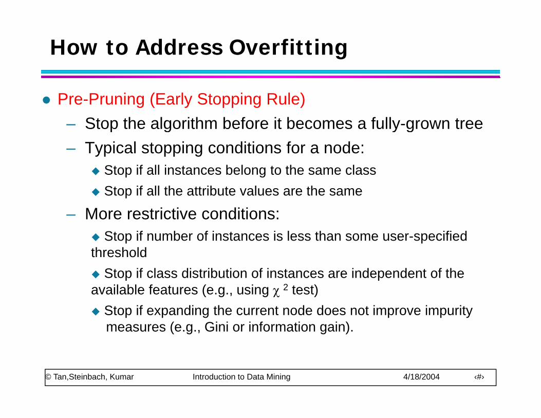
Pre-Pruning (Early Stopping Rule)– Stop the algorithm before it becomes a fully-grown treep g y g– Typical stopping conditions for a node:

Stop if all instances belong to the same classStop if all the attribute values are the same

– More restrictive conditions:Stop if number of instances is less than some user specifiedStop if number of instances is less than some user-specified

thresholdStop if class distribution of instances are independent of the

available features (e g using χ 2 test)available features (e.g., using χ 2 test)Stop if expanding the current node does not improve impuritymeasures (e.g., Gini or information gain).


How to Address Overfitting…

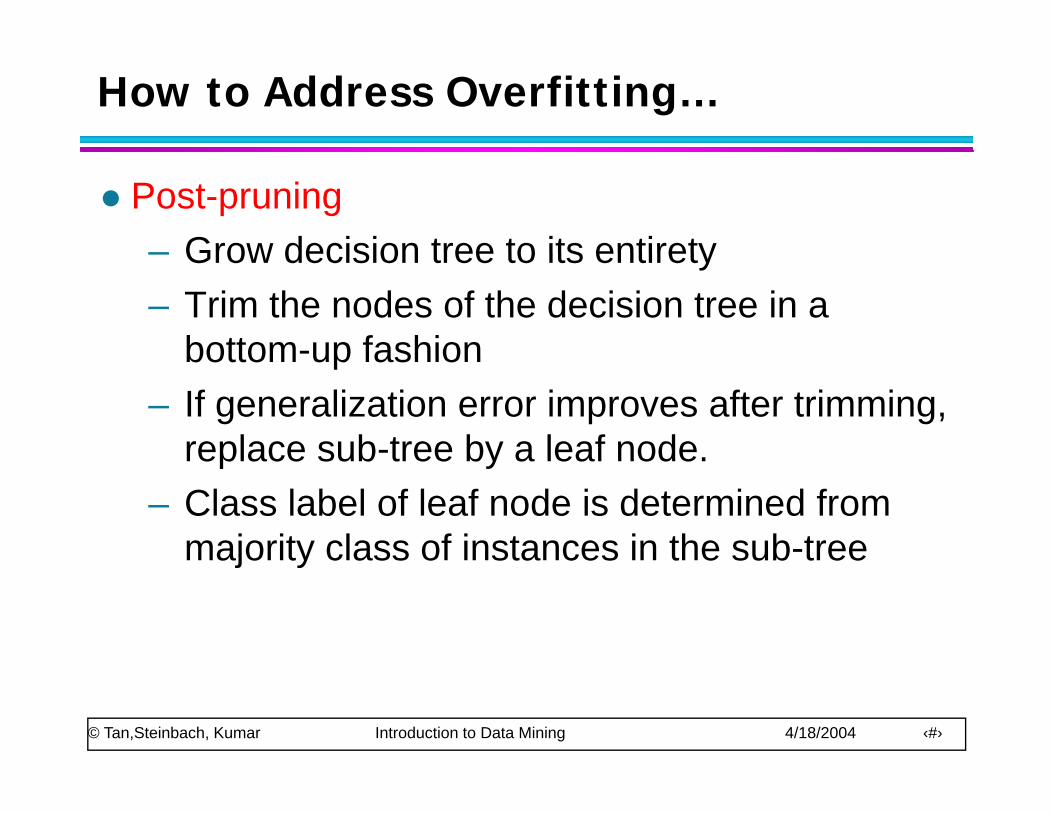
Post-pruning– Grow decision tree to its entirety– Grow decision tree to its entirety– Trim the nodes of the decision tree in a

bottom-up fashionbottom up fashion– If generalization error improves after trimming,

replace sub-tree by a leaf node.replace sub tree by a leaf node.– Class label of leaf node is determined from

majority class of instances in the sub-treeajo ty c ass o sta ces t e sub t ee


Example of Post-Pruning

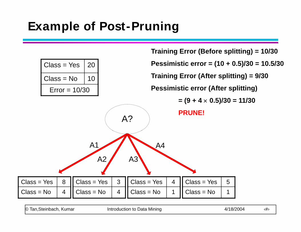
Class = Yes 20

Training Error (Before splitting) = 10/30

Pessimistic error = (10 + 0.5)/30 = 10.5/30

Class = No 10

Error = 10/30

Training Error (After splitting) = 9/30

Pessimistic error (After splitting)

= (9 + 4 × 0 5)/30 = 11/30

A?

= (9 + 4 × 0.5)/30 = 11/30

PRUNE!

A1

A2 A3

A4

A2 A3

Class = Yes 8 Class = Yes 3 Class = Yes 4 Class = Yes 5


Class = No 4 Class = No 4 Class = No 1 Class = No 1

Model Evaluation

Metrics for Performance Evaluation– How to evaluate the performance of a model?– How to evaluate the performance of a model?

Methods for Performance EvaluationMethods for Performance Evaluation– How to obtain reliable estimates?

Methods for Model Comparison– How to compare the relative performance

among competing models?


Model Evaluation

Metrics for Performance Evaluation– How to evaluate the performance of a model?– How to evaluate the performance of a model?

Methods for Performance EvaluationMethods for Performance Evaluation– How to obtain reliable estimates?

Methods for Model Comparison– How to compare the relative performance

among competing models?


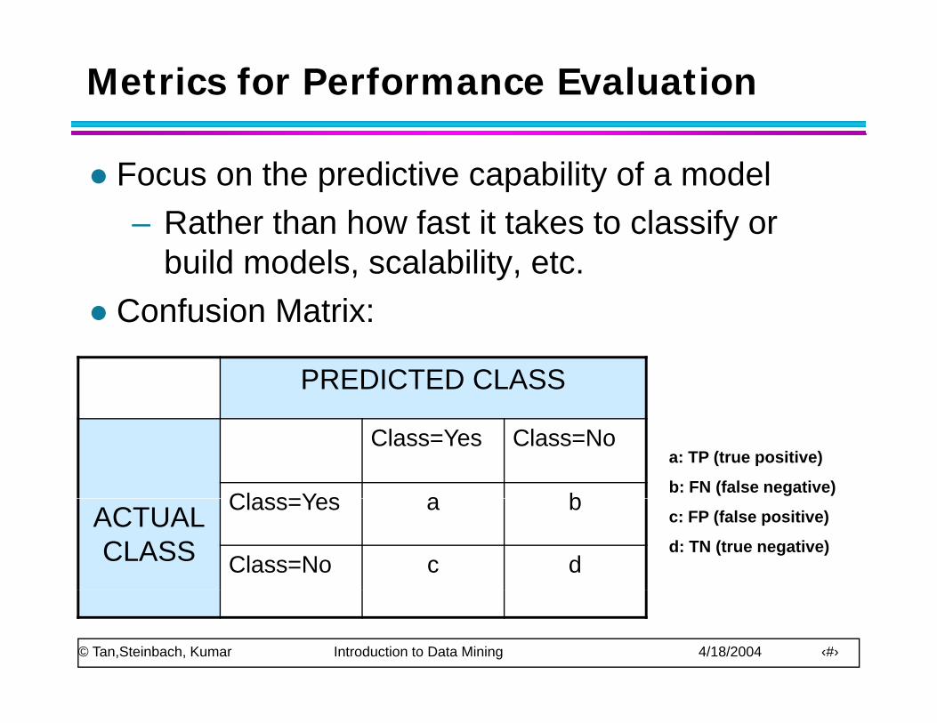
Metrics for Performance Evaluation

Focus on the predictive capability of a model– Rather than how fast it takes to classify or– Rather than how fast it takes to classify or

build models, scalability, etc.Confusion Matrix:Confusion Matrix:

PREDICTED CLASS

Class=Yes Class=No

Class=Yes a b

a: TP (true positive)

b: FN (false negative)

ACTUALCLASS

Class=Yes a b

Class=No c d

c: FP (false positive)

d: TN (true negative)


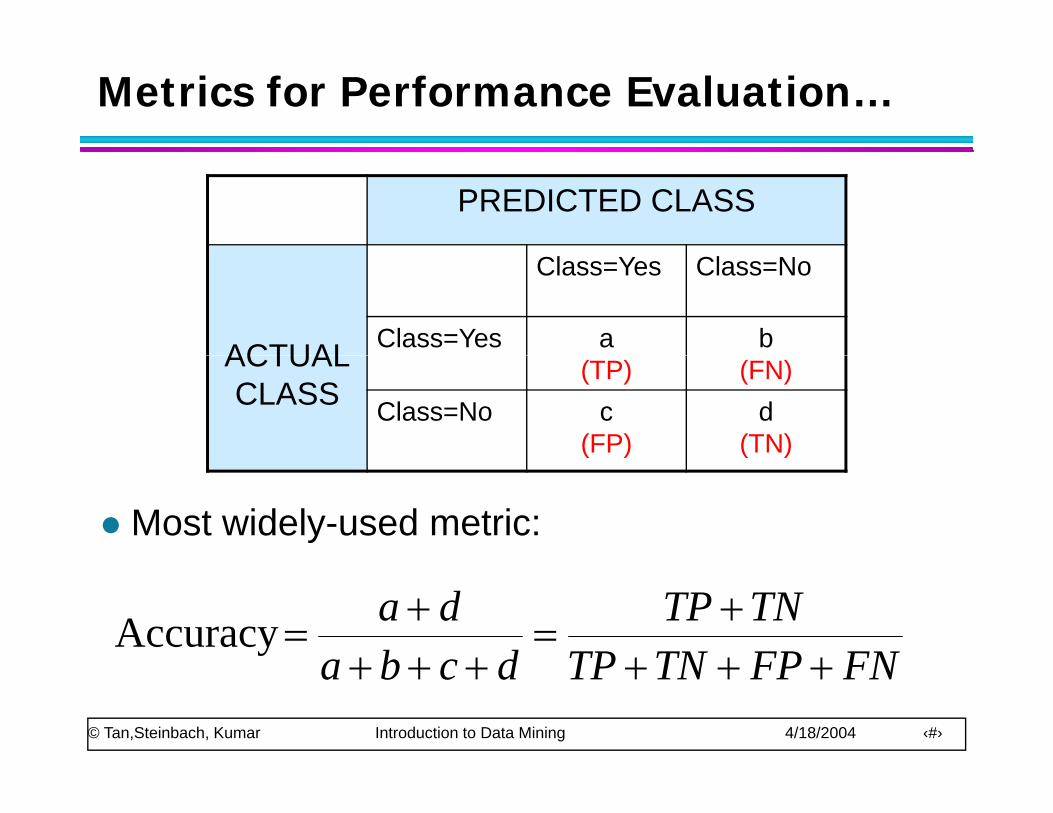
Metrics for Performance Evaluation…

PREDICTED CLASS

ACTUAL

Class=Yes Class=No

Class=Yes a bACTUALCLASS

(TP) (FN)Class=No c

(FP)d

(TN)

Most widely-used metric:

( ) ( )

FNFPTNTPTNTP

dcbada

++++

=+++

+=Accuracy


FNFPTNTPdcba ++++++

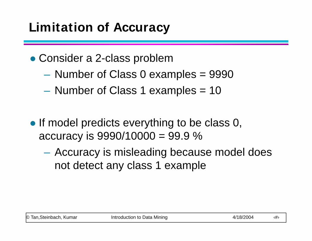
Limitation of Accuracy

Consider a 2-class problem– Number of Class 0 examples = 9990– Number of Class 0 examples = 9990– Number of Class 1 examples = 10

If model predicts everything to be class 0, accuracy is 9990/10000 = 99 9 %accuracy is 9990/10000 = 99.9 %– Accuracy is misleading because model does

not detect any class 1 examplenot detect any class 1 example


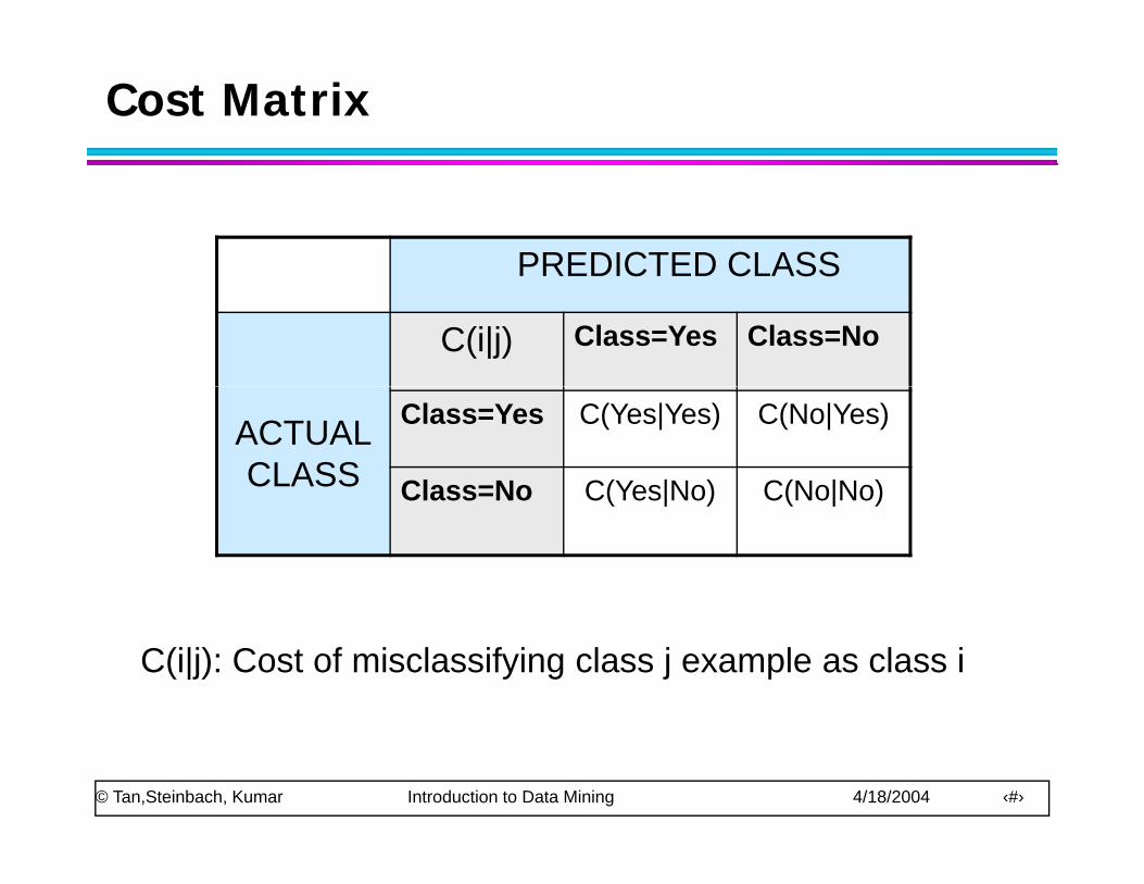
Cost Matrix

PREDICTED CLASSPREDICTED CLASS

C(i|j) Class=Yes Class=No

ACTUALCLASS

Class=Yes C(Yes|Yes) C(No|Yes)

Class=No C(Yes|No) C(No|No)Class No C(Yes|No) C(No|No)

C(i|j): Cost of misclassifying class j example as class i


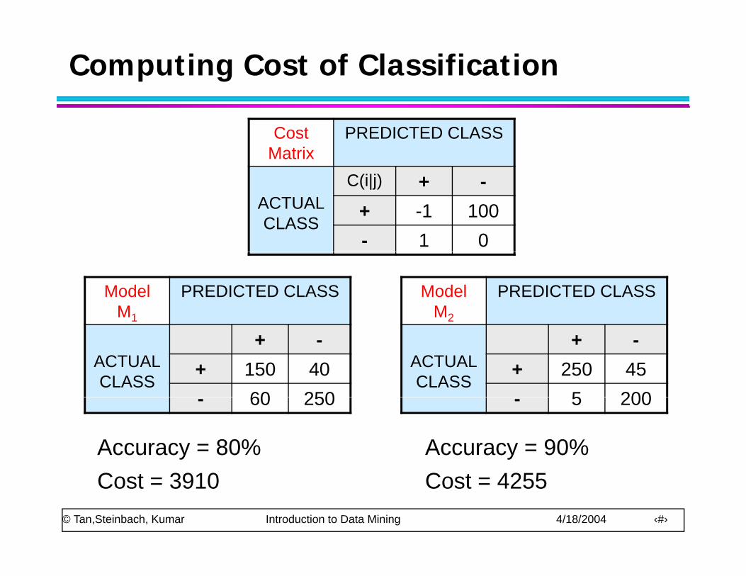
Computing Cost of Classification

Cost Matrix

PREDICTED CLASS

C(i|j) +ACTUALCLASS

C(i|j) + -+ -1 100- 1 0

Model M1

PREDICTED CLASS Model M2

PREDICTED CLASS

ACTUALCLASS

+ -+ 150 40

60 250

ACTUALCLASS

+ -+ 250 45

5 200- 60 250 - 5 200

Accuracy = 80% Accuracy = 90%


Cost = 3910 Cost = 4255

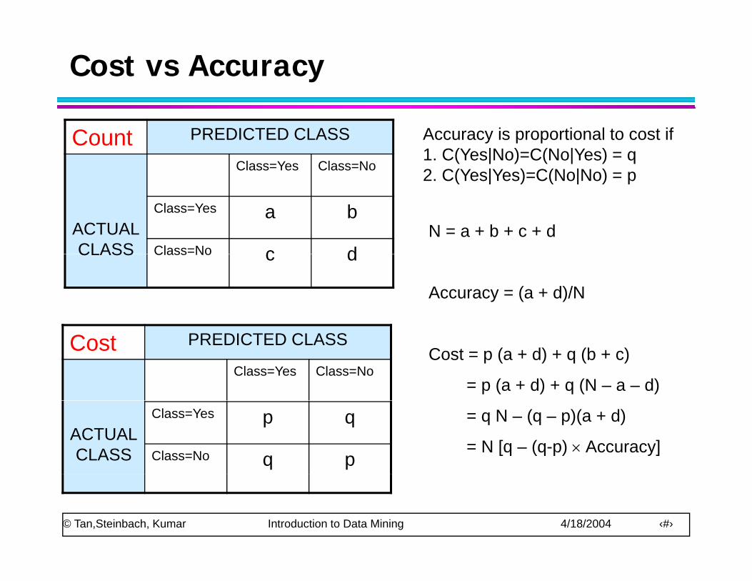
Cost vs Accuracy

Count PREDICTED CLASS

Class=Yes Class=No

Accuracy is proportional to cost if1. C(Yes|No)=C(No|Yes) = q 2. C(Yes|Yes)=C(No|No) = p

ACTUALCLASS

Class=Yes a b

Class=No c dN = a + b + c + d

2. C(Yes|Yes) C(No|No) p

CLASS Class No c d

Accuracy = (a + d)/N

Cost PREDICTED CLASS

Class=Yes Class=NoCost = p (a + d) + q (b + c)

= p (a + d) + q (N – a – d)

ACTUALCLASS

Class=Yes p q

Class=No q p

= q N – (q – p)(a + d)

= N [q – (q-p) × Accuracy]


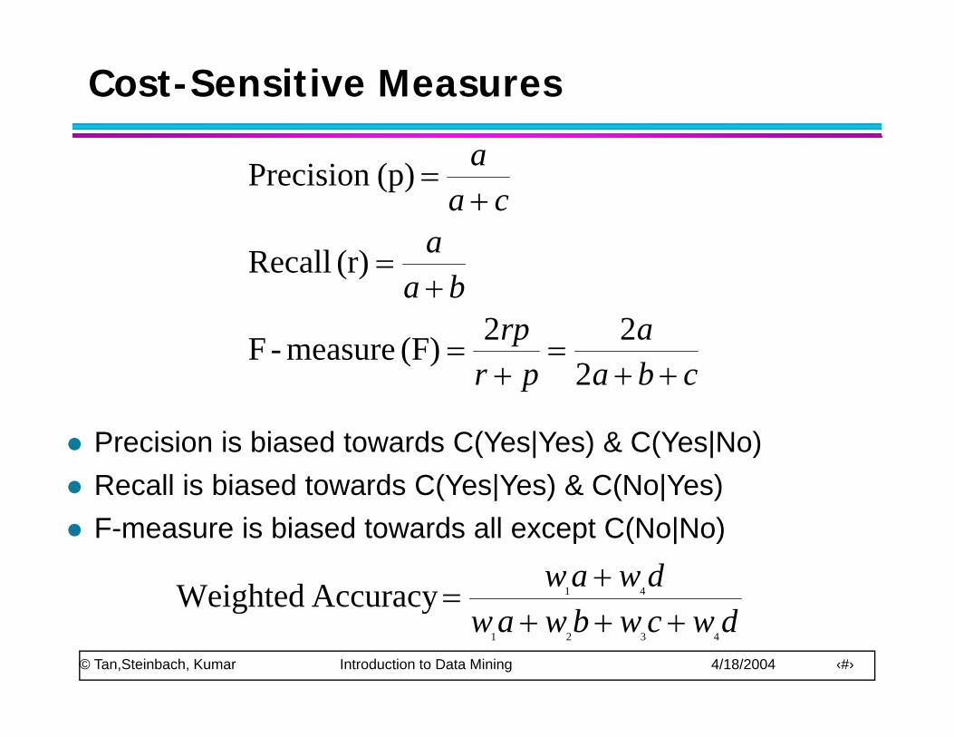
Cost-Sensitive Measures

caa+

= (p)Precision

baa+

=

22

(r) Recall

cbaa

prrp

++=

+=

222(F) measure-F

Precision is biased towards C(Yes|Yes) & C(Yes|No)Recall is biased towards C(Yes|Yes) & C(No|Yes)F-measure is biased towards all except C(No|No)

dwaw41AccuracyWeighted +

=


dwcwbwaw4321

Accuracy Weighted+++

=

Documents

Decision Tree Induction