Embed Size (px)
Citation preview

Univers
ity of
Cap
e Tow
n
i
Decision Tree Classifiers for Incident Call Data Sets
by
Igboamalu Frank Nonso
Supervised by
Assoc. Prof Sonia Berman
MINOR DISSERTATION PRESENTED IN PARTIAL FULFILLMENT
OF THE REQUIREMENTS FOR THE DEGREE OF
CONVERSION MASTERS IN INFORMATION TECHNOLOGY
IN THE DEPARTMENT OF COMPUTER SCIENCE
UNIVERSITY OF CAPE TOWN
September 2016

The copyright of this thesis vests in the author. No quotation from it or information derived from it is to be published without full acknowledgement of the source. The thesis is to be used for private study or non-commercial research purposes only.
Published by the University of Cape Town (UCT) in terms of the non-exclusive license granted to UCT by the author.
Univers
ity of
Cap
e Tow
n

ii
Plagiarism Declaration
I know the meaning of plagiarism and declare that all of the work in the
document, save for that which is properly acknowledged, is my own.
Igboamalu Frank Nonso

iii
ACKNOWLEDGEMENTS
I would like to express my gratitude to my supervisor, Assoc. Professor Sonia
Berman, for her guidance and support during this process, thank you for being the best and
most supportive supervisor ever.
Many thanks to my family; your support and encouragement have been instrumental
throughout my dissertation. To my brothers Dr. Chris, indeed you are really a brother and a
friend, thanks for the motivation. Henry Emeka (Awkudon) and Engr Tony of a truth you
guys really surprised me, Thank you for the love and for always believing in me. To my
lovely wife Dr. Ugo and my beautiful daughter Goziem, this work wouldn't have been
possible without you people during the toughest moments when I thought I will not make it
again, thanks for your love, support, and encouragement I am really grateful. There are not
enough words to express my gratitude to my parents Chief and Mrs. F C Igboamalu, thanks
for your spiritual support and encouragement. I love you all.
Lastly, the financial assistance from the NRF towards completion of this dissertation and the
oil and gas company that provided the data for my experiments is hereby acknowledged.
.

iv
Abstract
Information technology (IT) has become one of the key technologies for economic
and social development in any organization. Therefore the management of Information
technology incidents, and particularly in the area of resolving the problem very fast, is of
concern to Information technology managers. Delays can result when incorrect subjects are
assigned to Information technology incident calls: because the person sent to remedy the
problem has the wrong expertise or has not brought with them the software or hardware they
need to help that user. In the case study used for this work, there are no management checks
in place to verify the assigning of incident description subjects.
This research aims to develop a method that will tackle the problem of wrongly
assigned subjects for incident descriptions. In particular, this study explores the Information
technology incident calls database of an oil and gas company as a case study. The approach
was to explore the Information technology incident descriptions and their assigned subjects;
thereafter the correctly-assigned records were used for training decision tree classification
algorithms using Waikato Environment for Knowledge Analysis (WEKA) software. Finally,
the records incorrectly assigned a subject by human operators were used for testing. The J48
algorithm gave the best performance and accuracy, and was able to correctly assign subjects
to 81% of the records wrongly classified by human operators.

v
Table of Contents Page
Plagiarism Declaration .........................................................................................................................ii
Acknowledgements.......................................................................................................................... iii
Abstract ....................................................................................................................................... iv
Table of Contents................................................................................................................................. vi
List of Tables .................................................................................................................................. vii
List of Figures............................................................................................................................ viii
Chapter 1 Introduction ........................................................................................................................ 1
1.1 Background ............................................................................................................................... 1
1.2 Problem Description ................................................................................................................. 3
1.3 Project Significance ................................................................................................................... 4
1.4 Research Questions ................................................................................................................... 4
1.5 Dissertation Outlines ................................................................................................................ 5
Chapter 2 Literature Review ............................................................................................................... 6
2.1 Data Mining .............................................................................................................................. 6
2.2 Supervised Learning (Classification) ........................................................................................ 7
2.3 Unsupervised Learning ............................................................................................................. 7
2.4 WEKA ...................................................................................................................................... 8
2.6 Decision Tree ............................................................................................................................ 9
2.6.1 Iterative Dichotomiser3 (ID3) ......................................................................................... 9
2.6.2 C4.5 ................................................................................................................................... 9
2.6.3 CART ............................................................................................................................. 10
2.6.4 NBTree ........................................................................................................................... 10
2.6.5 Random Forest ................................................................................................................ 10
2.6.6 Random Tree .................................................................................................................. 11
2.6.7 REPTree .......................................................................................................................... 11
2.7 Related Work ............................................................................................................................ 9
2.8 Conclusion .............................................................................................................................. 13
Chapter 3 Methodology .................................................................................................................... 14
3.0 Research Methodology ........................................................................................................... 14
3.1 Data Source ............................................................................................................................. 15
3.2 Data Preparation ..................................................................................................................... 17
3.3 Data Transformation ................................................................................................................ 18

vi
3.3.1 Data Normalization ............................................................................................................ 19
3.4 Data Source Analysis (exploration) in Excel .......................................................................... 20
3.5 WEKA Implementation .......................................................................................................... 24
3.5.1 Data loading in the WEKA .............................................................................................. 24
3.5.2 Format for WEKA File ................................................................................................... 25
3.5.3 Visualization of Input File .............................................................................................. 28
Chapter 4 Experimental Result ......................................................................................................... 30
4.1 Distinguishing Training and Test Data ................................................................................... 30
4.1.1 Train and Test "ORIGINALLY-RIGHT" File .................................................................... 31
4.2 WEKA Model Training Results ............................................................................................. 32
4.3 WEKA Test Result ................................................................................................................. 34
4.4 Second Approach using Decision Tree ................................................................................... 40
4.5 Test Results of Second Approach ........................................................................................... 43
Chapter 5 Conclusion ....................................................................................................................... 45
5.1 Conclusion and Discussion .................................................................................................... 45
5.2 Future Work .......................................................................................................................... 47
References .................................................................................................................................... 50

vii
LIST OF TABLES
Table Page
1 Summary of Keyword Counts 21
2 Summary of Subject Occurrences 22
3 WEKA decision tree results using 10-fold cross-validation 32
4 Classifier Accuracy 33
5 Time Taken to Build Model for Training Data 34
6 Predicted Result 38
7 System Confidence Levels 40
8 System Performance 40
9 Time taken to Build Model using Second Approach 43
10 Predicted Result for Test Cases using Second Approach 44

viii
LIST OF FIGURES
Figure Page
1 The Training and Testing of a decision tree classifier 15
2 A Sample of Incident Data 16
3 Sample of Input given WEKA 26
4 Sample of 36 attributes loaded on WEKA Explorer 27
5 Visualize All Data in WEKA Explorer 29
6 Sample of Input ORIGINALLY-WRONG File ARFF to WEKA 36
7 Test Set 37
8 Confidence Value Analysis 39
9 Alternative Approach: Decision Tree for Mouse 41
10 Alternative Approach: Decision Tree for Lotus 42

ix
LIST OF ABBREVIATIONS
SVM Support Vector Machines
MLR Multinomial Logistic Regression
IT Information technology
WEKA Waikato Environment for Knowledge Analysis
OGA Oil and Gas Company in Africa
CART Classification and regression trees
NBTree Naive Bayes Tree
ID3 Iterative Dichotomiser 3
LADtree Logical Analysis of Data
Problemsubject Subject of the problem

1
Chapter 1
Introduction
1.1 Background
One of the goals of an Information technology (IT) service organization is to ensure service
availability and that User Incidents (IT problems) are resolved. User Incidents are usually
communicated via “Incident Calls”. These typically contain a description of the problem and are
stored or archived for future reference.
When incident calls are received they are allocated a Subject by a human operator, which is
used by the IT service personnel to see who should attend to the incident and what hardware and
software they should take with them when doing so. Often times, these subjects are wrongly assigned
due to human mistake, wasting time for both IT staff and the other staff who are waiting for the
incident to be resolved. This wastes time because the wrong person, hardware and/or software is sent
to fix it. One area of opportunity is to build a system that will be able to classify incidents based on
their description.
Data mining algorithms can be seen as a knowledge management technique and as one of the
decision-making tools to help solve the problem for IT Incident Calls classification. There are many
Data mining tools which are available for Data mining [1][2]. Among the many classification

2
algorithms, Decision Trees are the most widely used. A Decision Tree is simple to understand and
interpretat, and requires little data preparation, compared with other techniques which usually require
data normalization [3,4]. It handles both numerical and categorical data. Moreover, a decision tree
analyses large data within a short period of time and its ease of execution can be applied to any
domain.
For a large-scale company like an Oil and Gas company in Africa (called OGA here for
privacy reasons) with more than five thousand users inside the company and ten thousand Incident
Calls per year, an important IT Service management objective is to ensure that a particular incident
description is properly assigned to the right subject that will allow handling the incident without any
delay.
This dissertation aims at using Decision Tree algorithms to determine the subject of
incident calls automatically, in order to compare the accuracy of these algorithms in relation
to each other and to the accuracy of human operators. If decision trees can assign subjects
more accurately than humans, this can help to speed up the time taken to resolve incident calls,
as desired by OGA’s IT manager. Generally, the impending problem faced by the company is that,
IT Incident Calls are not managed appropriately, in the sense that often, there are no management
checks in place to verify the way the Incident subject is assigned despite its importance for
productivity. But instead, many problems are assigned to a wrong subject and this repeats itself after
a particular time interval. The task then is, how to control each Incident Call, to make sure that the
problem was assigned the right Subject, and this research will compare the accuracy of various
decision tree algorithms and see if these can correctly assign subjects where human operators had
failed to do so.

3
In this dissertation, the analysis will be carried out using different Decision Tree algorithms
for classification, namely J48, RandomTree, RandomForest, REPTree, NBTree, LADTree, J48Graft,
SimpleCart [3, 4] for classifying IT incident calls. As a secondary goal, the performance will also be
analyzed in terms of time taken to classify the IT Incident data set.
1.2 Problem Description
The main problem this dissertation is addressing is how to correctly classify incident calls
which will eliminate wrong assignment of subjects to problems due to human mistake. This would
include analysing subjects that were manually assigned to problems and developing a trained model
that will automatically do the task.
Usually assigning subjects to incidents is slow and often inaccurate, because the incident
subject is manually assigned, which often leads to errors due to the human factor. This research,
therefore, addresses the following question: Can a semi-/automated system improve subject
assignment accuracy and speed, using a decision tree learning from past incident call data? Such a
system was built and the OGA stored data was used to see if accuracy had improved and
performance/speed was of an acceptable standard. This Automated Incident call system receives an
email as input, and provides as output the subject and personnel to fix it. The need for such a system
has been noted elsewhere [53] [54]. In the light of the aforementioned problem, this dissertation will
consider and assess different widely used decision tree algorithms and recommend one that is the best
fit to the current problem faced by OGA.

4
1.3 Project Significance
A correctly assigned Subject for an incident description from IT knowledge base management
will be very helpful in resolving the issue. In addition, the automatic way to assign a subject aims to
make the process of resolving the IT incident calls easier, faster, save down time and improve
efficiency for the company as a whole. This would be beneficial not only to the IT department who
are responsible for the improvement of IT service management, but also to the entire company and
can potentially find a solution that can be used in other companies.
1.4 Research questions
The following research questions will be addressed:
Can an automated system assign a subject to IT incident calls with acceptable accuracy?
Can this assign correct subjects to those calls where humans were incorrect?
Which decision tree algorithm is best for this in terms of accuracy and performance?
The major aim of this dissertation is to train a system that can automatically do this job
(assigning the incident a subject in order to know which IT personnel/subject should handle it). This
will save an employee from having to do it, and will hopefully be as accurate as that person or better.
For past decades, a number of decision tree algorithms have been proposed such as ID3, J48,
CART, C4.5, C5.0, IDE, Random Tree, Random Forest and SLIQ [51]. But the most common
algorithms for numerical values, which this work aims at comparing are J48, J48 Graft, Random Tree,
Random Forest, NBTree, REPTree, LADTree, and SimpleCart [52].

5
1.5 Dissertation outline
This dissertation is organized as follows; In Chapter 1, the problem statement, objective,
research question and project significance were presented. Chapter 2 is the literature review which
gives an overview of Data Mining, Supervised learning (Classification), Decision Trees, ID3, C4.5,
CART, NBTree, Random Forest, Random Tree, REPTree and other related work. In Chapter 3, the
methodology of this investigation is explained. Chapter 4 provides the results of the study and Chapter
5 presents the conclusion and further work.

6
Chapter 2
Literature review
2.1 Introduction
One of the important roles of IT incident management is to keep IT services working
and ensure that quality of service is optimal without experiencing any down time. The IT database
contains information that is used to manage IT incident calls properly. The data set from the IT
database can be used to predict the possible subject or personnel to which the incident call will be
assigned to avoid increasing down time. Classification of IT incident call data could be a data
mining task that can group similar data together to determine a suitable solution for a specific
issue. Decision trees a r e an important tool for classification of data in a data set [43].
IT incident management has become complex over time, with added pressure from
severely constrained resources, expectations that incident calls b e r e s o l v e d without much
delay and using increasingly complex new technologies. Classifying of IT incident calls are just
one of the trends that are creating new challenges [44]. This is because IT incidents are not
a l w a y s managed appropriately a n d o f t e n do not have any form of a check for the re-
occurrence of calls that were assigned a wrong subject due to human error, so instead this problem
repeats itself after a particular time interval. The issues then are how to control each incident call
to make sure that the calls are assigned properly and can be resolved at once.
The primary goal of this dissertation is to compare the classification performance and to
find the best algorithm using various decision trees to predict incident calls Subjects in a corporate
environment. In this study, we are not trying to build another toolkit for classification of IT
incident calls. Rather, we hope to define the way we can classify IT incident description using
tools such as ID3, C4.5, and CART. The one with the best performance will be used to classify
the incidents in a semi-/automated system.
In this chapter, the first section will cover the introduction aspect of decision trees in which
various techniques of a decision tree and its working process w i l l b e analyzed and summarized.
In the end application of decision, tree techniques will be presented from different research sources.

7
2.2 Data mining
Data mining which is also known as knowledge discovery in databases or database
mining [5] can be simply defined as a process of analyzing a large data set to discover patterns and
relationships. These can be achieved using the data mining technique which is the classification
of data and prediction. There are different methods of data mining such as Supervised learning
(e.g/ classification), Unsupervised learning (e.g. clustering), Association Rules, Data
Generalization, Regression, Dependency modeling. This chapter will focus on supervised learning
which is within the scope of this work.
2.3 Supervised Learning (Classification)
The main objective of classification [ 6 ] in data mining is to achieve error free
assignment of each record in a data set to one of a limited number of possible categories. The
working principle of classification is that firstly a model will learn from a given data set how to
determine each record’s class in terms of its attributes and then the model will use this for class
prediction. Classification is, therefore, a model for identifying the class attribute as a function of
the values of other attributes [42]. There are many techniques for classification such as Decision
Trees, Neural Networks, Bayesian Networks and many others. This research focuses on the
decision tree algorithm. Supervised learning is the type of learning that that makes use of classes
or categories already given to existing data, which are utilized for training purposes [27].

8
2.4 Unsupervised learning
Unsupervised learning is the ability of a data mining algorithms such as a neural network to
learn and structure data without any provision of an error signal to evaluate the solution [27] i.e. the
learning is done heuristically. The unsupervised learning normally generates its own representation
of input data for patterns classification. Some techniques for unsupervised learning are self-organizing
maps, competitive learning [30] and adaptive resonance theory [31].
2.5 WEKA
The WEKA (Waikato Environment for Knowledge Analysis) machine learning tool [34] [35]
can be used for performing clustering and classification. WEKA is referred to as open source software
[37][38] because it can be modified since its design or source code can be accessed publicly, it is free
to use without payment, it is very flexible, and it has security and accountability. Because WEKA
executes a large collection of machine learning algorithms, it is widely used for exploring large
amounts of data [36].
In this dissertation, we focus on data classification and the WEKA Explorer includes a classify
tab which enables a user to apply classification and regression algorithms to a dataset. It will also
analyze the correctness of the resulting predictive model.

9
2.6 Decision Trees
Decision trees are useful and powerful tools in classification and prediction [45]. Decision
trees are the most popular data mining technique compared with other data mining techniques for
knowledge discovery. “Decision tree learning is one of the most widely used and practical
methods for inductive inference” [7]. A decision tree is structured in a way that breaks down a
data set into smaller subdivisions known as internal nodes and leaf nodes. The internal node is the
type of node that can split into two or more parts. An internal node has two or more branches, each
branch representing values for the attribute tested. The leaf node is the type of node that contains a
tag or label (classification) that means it does not require additional classification testing. A branch
is a connection between two nodes; it can be from an internal node to an internal node or from an
internal node to a leaf node. Decision trees have many advantages over other classification methods
such as they are easy to use, the rules in the decision tree are easy to understand and the tree size is
independent of the database size in terms of scale [32] [33].
2.6.1 Iterative Dichotomiser3 (ID3)
ID3 is a decision learning and mathematical algorithm which Quinlan Ross introduced
in1986 [8]. The ID3 algorithm [9][10] basically builds a tree based on information theory from the
top down without retracing to the top, known as the root. It starts the greedy algorithm from a fixed
set to test each attribute at every tree node. It is based on Hunt’s algorithm. ID3 makes use of
information theory which was introduced by Shannon in 1948. ID3 uses the concept of entropy
[15] and information gain [16][17] to help to select the attribute that is most useful for attribute
classification. Information gain is the amount of information needed to classify an item before a
particular split minus the amount needed to classify an item after that split [46]. ID3 uses binary
splits.
2.6.2 C4.5, J48 and J48 Graft
C4.5 is an extension of ID3 [12] and very popular among classification tree methods. It
is an improvement from ID3 [8] [11] to include continuous values and handle missing values so

10
that it can be able to avoid over-fitting. C4.5 uses multi-way splitting to reduce the size of the
decision tree. Pruning is one of the functions that make C4.5 different from ID3, as is the
introduction of the gain ratio w h i c h evaluates information g a i n e d from a split. Unlike
information gain, information gain ratio is not affected by how many values an attribute can take on
i.e. is not affected by domain sizes. Since the emergence of C4.5, WEKA’s J48 algorithm was
developed which implements the C4.5 algorithm using binary splits. The J48Graft algorithm extends
this by adding a post-processing step to the algorithm, which adds new nodes to the tree in order to
improve accuracy at the cost of greater tree complexity.
2.6.3 CART
CART means Classification and Regression Trees; it was y developed by Breiman [13]. In
CART, numeric and categorical attributes are used to build decision trees and it also has features
for missing attribute values built in [14]. CART is a binary tree that uses information gain at each
node [50]. CART selects a discrete value to split on at each internal node in a greedy way that
makes it very sensitive to its training data.
2.6.4 NBTree
The Naïve Bayesian tree learner, NBTree [17], is the combination of Naïve Bayesian
classification and decision tree learning. The NBTree has a similar algorithm learning to C4.5. It uses
the data associated with that leaf to construct a naïve Bayes for each leaf when the tree is grown.
NBTree performs better in terms of higher accuracy compared with decision tree learners or Bayesian
classifiers alone [47].
2.6.5 Random Tree and Random Forest
A random tree [19] is a tree that selects a random subset of attributes to consider at
each node. It performs no pruning i.e. it does not simplify a tree by combining nodes during or after
the training process. A random forest is an ensemble learning method for classification or regression
using multiple random trees [18]. It builds random decision trees from different subspaces of the
feature space and then uses bagging (averaging or voting by these trees) in prediction. This is a way
of handling the overfitting problem when using one decision tree so that random forests can improve

11
performance over a single-tree classifier. Its accuracy depends on the strength of the individual trees
in the forest and the correlation between them.
2.5.6 REPTree
A REPTree is one of the fastest decision tree learners [49], its builds a decision/regression tree
using information gain as the splitting criterion, and uses reduced-error pruning (REP). REP involves
replacing a node by its most popular child node in such a way as to minimize the error from the
variance. It only sorts numeric attributes once, in order to improve performance. Missing values are
dealt with using the C4.5’s method of splitting items into separate instances.
2.6.7 LADTree
By using boosting, an alternating decision tree algorithm builds a tree where nodes are alternately
prediction nodes and decision nodes. Boosting gives different weightings to different instances. At
first, all instances have the same weight, but the weight of an instance is increased whenever it is
correctly classified and is decreased whenever it is wrongly classified. The LAD Tree extends the
alternating decision tree algorithm to deal with non-binary classification [48].
2.7 Related Work
In [20], the authors conducted an experiment with four algorithms which included ID3, J48,
SimpleCart and Alternating Decision Tree on the spam email dataset in which they make used of the
WEKA environment and they were able to compare them in terms of classification accuracy. They
concluded from their simulation results that the J48 classifier performed better than the ID3, CART,
and ADTree in terms of classification accuracy.
In [21], the authors conducted a n experiment on eight different classification algorithms

12
and conducted a comparative test in which they obtained their optimum algorithm for students’ data
set classification. They made use of the WEKA-knowledge analysis tool for their simulation
measurement. They used the classification technique to measure potential s o a s to significantly
improve performance; i t was suggested for use in colleges’ admission and enrolment applications.
According to their results, it can be concluded that C4.5, CART and Random Forest algorithms were
able to produce the highest performance and accuracy compared with the IBK-E and IBK-
Algorithms which produced more errors.
O t h e r research o n qualitative data of a student [22] compared performance using decision tree
algorithms ID3, C4.5, and CART. From their research, it was observed the use of Gini Index for
attribute selection in CART together with the information Gain Ratio is better than that of ID3 and
C4.5. CART had higher prediction accuracy when compared with that of ID3 and C4.5. However,
the classification accuracy difference for the decision tree algorithms is not considerable. It
can also be concluded from their experimental results that students’ performance was
affected by qualitative factors such as emotional factors.
An algorithm which predicted the performance of a learner using decision trees and genetic
algorithms [23], used the ID3 algorithm to provide multiple decision trees. Each decision
tree predicts the performance of a student in terms of different attributes. As each decision
tree provide clear insights which were different for different trees, they were able to predict
performance and also to identify the key attributes that influence the result. The genetic
algorithm was implemented for calculating the performance of each tree and introducing the
process of crossover operations in multiple generations, which as generation increased
created trees with a better fitness.
In the classification of short-term urban traffic flow, [24], make use of decision tree

13
algorithms such as CART, C5.0, QUEST, and CHAID, where input variables are multiple roads'
traffic flow values. The predicted variable is a certain road's condition 5-30 minutes later. The
C A R T a l g o r i t h m was better than the others based on the experimental result. From their
ex p e r i m en t , it could also be seen t h a t C A R T and CHAID trees were more concise and
understandable with fewer nodes.
A case study to predict the performance of students in the examination [25] used WEKA
C4.5, I D 3 , a n d CART decision tree algorithms. The decision tree predicted the number of
students who are likely to pass or fail. Their results provided steps for improvement of
performance of the students who were predicted to fail
In [26] research on a comparative study of the decision tree, ID3 and C4.5 is given. Initially,
the classical algorithm of ID3 was presented, then they discussed in more detail that C4.5 is the
natural extension of the ID3 algorithm. They also compare these with different decision tree
algorithms which included C5.0 and CART.
2.8 Conclusion
Data mining tools automatically detect information from raw data using data mining
algorithms. Data mining algorithms differ from each other in terms of the way they analyze raw data.
As an example CART, ID3, C4.5, and C5.0 differ in the way splits are performed, and CART is a
binary tree whereas the others are not. Each algorithm gives a unique decision tree from the input
data as discussed above.
In this study, we have investigated decision tree classification of incident calls using the
different algorithms described here, as these are the suite of decision trees provided in the WEKA
environment. Unlike previous work, this project focuses on a data set from an IT database of incidents

14
calls w h i c h w i l l b e analyzed using different decision tree algorithms t o c o m p a r e
performance and accuracy.

15
CHAPTER 3
METHODOLOGY
This chapter will outline the research process thereby providing the rationale for the
research methodology which was chosen. It will also demonstrate the proposed model for
classification and automatic assignment of Subjects based on incident descriptions in the Oil
and Gas Company case study.
3.0 Research Methodology
The Figure 1 flow chart outlines the methodology dissertationfolllowed. dissertationThis
firstly involves the normalization of text data, the Incident Description, so as to extract the correct
Subject. This normalization reduces the training error during data classification. Secondly a python
code program reads the archive incident data from an input file, line by line, and writes the
ProblemSubject of each line to the output file. Decision trees were investigate to learn from past
experience (training phase) and to then predict Subjects for new incident descriptions (test phase).

16
Archive data gathered from IT Help desk
Test DataPredicted
subject. No or
identical.
Confidence Levels
is use to get the
best subject
Subject prediction by decision tree
Data Normalization
using python
Set the confidence
level to max at
which that subject
was predicted
Yes Correct assigned by Human
Test and Training
Data Test
Data Mining
Selestion
J48
Classifier
Rando
m Tree
Rando
m
Forest
REPTree NBTree J48GraftLADTr
ee
Simple
Cart
Training and Test data using ProblemSubject and ResolvedSubject
No Wrong Assigned by Human
35 Subject classification and confidence level
Subject Output and confidence level
Figure 1. The Training and Testing of a decision tree
classifier.
3.1 Data Source
The IT Incident data relies mostly on the problems faced by users. The incident data
information is entered into a database with the help of an incident management system interface. The
data set used in this dissertation was collected from IT incident call's repository in the user support
department of an African Oil and Gas Company from 2009 to 2014 as shown in figure 1 below

17
Sample of Incident Dataset
Figure 2 A Sample of Incident Data

18
The total sample data collected was 22521 records. However, each record is composed of Incident
description and several other attributes including the Subject assigned to the incident (called
“ProblemSubject”) and the Subject assigned to the incident after it had been solved (called
“ResolvedSubject”). The original data was studied and analyzed using Excel to compare
ProblemSubject with ResolvedSubject, where it was realized there were many that were wrongly
assigned their ProblemSubject. The data was therefore divided into two sets, one where
ProblemSubject matched ResolvedSubject (correct assignments) and the other where they did not
match (wrong assignments). The system was trained using WEKA software on those that were correct
and tested on those that were incorrect. This turned out to mean training on 90% and testing on 10%.
3.2 Data preparation
The goal of this work was to analyze the incident description in order to correctly classify
which Subject to assign to that call. Since descriptions used are texts from email, only keywords from
the texts were used for this purpose. That is, the aim was to create a system that learns from past data
that “this type of problem sent to the helpdesk” leads to “this/these most likely keywords” and assign
the incident to the subject/personnel that will handle the incident. Then in future whenever a help
email arrives, it can be fed into the system and the system displays the likely subject and the helpdesk
personnel who will handle the incident.
At first information from the database was carefully analyzed using Weka and different
combinations of attributes were used to predict the subject. However, at the time of Subject
assignment, only the User and the Description exist, so keywords within Description were used.
Because the data mining system is built to help by suggesting a likely Subject before the problem is
handed over to staff to be resolved, it should only work with data that is known before the problem
has been attended to. And this can only be Incident Description and whoever emailed this to the

19
helpdesk i.e. User Status. However, an initial analysis showed that User Status was not useful in
predicting an incident's Subject, since the status only gave information on whether the user was
permanent staff or contract staff.
Therefore Incident Description was used as input to the final product or model that the data
mining produces. It was thus necessary to investigate decision trees learning from past experience
how to predict Subjects based on an incident description. Data exploration gave rise to an initial set
of 44 ProblemSubjects being replaced by 35 ProblemSubjects to bring these in line with
ResolvedSubjects. It also led to data being divided into 2 files: ORIGINALLY-RIGHT and
ORIGINALLY-WRONG, which will be discussed in the next section.
In this dissertation, the first problem addressed is normalization of text data, the Incident
Description, so as to extract the correct Subject. Incident description keywords are used for this, by
making each keyword a separate attribute in a new database. Its value for a particular Incident
Description is the number of times that a keyword (e.g. VCR or Acrobat etc) appears in that Incident
Description. So, for example, the first complete Incident description in the spreadsheet is "Install and
activate the digital telephone box and extension for the Church gate 3rd-floor meeting room. - The
extension should have telephone-National access. DETAILS: Location: 305 Church Gate Lagos.
Description: 305 REGINA Meeting room. Tel Ext: 6846. Contact Odu for any desired detail." The
keyword “telephone” appears twice and the keyword “install” appears once. There is thus more than
one keyword, and the actual Subject is Telephone, which occurs more often than Install. It would thus
have a value of 1 for (keyword attribute) Install and a value of 2 for (keyword attribute) Telephone,
and a value of 0 for all the other keyword attributes. The expectation is that a decision tree will learn
from such keyword frequencies which Subject to assign to an incident.

20
3.3 Data Transformation
The fields that are required for data mining were derived using Python code to count keywords
in the information extracted from the database. For the training step, only ORIGINALLY-RIGHT
records were used. That is the training data comprised incident descriptions of only those calls which
the human operator had classified correctly – choosing a ProblemSubject to assign to it which exactly
matched the ResolvedSubject later given by the person who fixed that problem.
The program reads the archived incident data from an input file, line by line, and writes the
ProblemSubject of each line to the output file. It picks up the Incident Description from each line and
passes each Incident Description to a counting function and also sends the counts that it returns to the
output along with the Subject of that training example.
The count function detects keywords and counts how many of each occurs in a
description. Thus each line of output from the Python program contains incident-ID, all keyword
counts, and assigned-subject. These counts are small integers, most of them zeroes. Subjects have
one or more keywords associated with them (e.g. keywords monitor and screen are both associated
with Subject “monitor”.) The final output has one count for each subject, which is the total of the
counts for all the keywords associated with that subject.
The algorithm is as follows:
(A) For Each Line in the Input File:
(A1) Read the Incident Number and write it to the output file, followed by a comma
(A2) Set all keyword counts to 0 (no keywords found in this incident description yet)
(A3) For each word W in the Incident Description do:

21
For each keyword K in the Keywords array do:
if W == K then add 1 to the count for keyword K
(A4) For each subject, total the counts of all its associated keywords
(A5) Write each of the counts to the output file in order, each followed by a comma
(A6) Read the Subject from the input file and write it to the output file
3.3.1 Data Normalization
The next step is to perform normalization of data. Normalization is one of the
techniques used for pre-processing of data, it helps standardizing the values of the input from varied
range to a particular range. Data normalization reduces the training error of data classification.
Normalization was needed in this work to check that the set of possible Subjects associated
with incidents by the human operator was changed to coincide with the set of possible
ResolvedSubjects associated with incidents by IT personnel after problems had been fixed. Then
keywords had to be explored to see which were the best to use for detecting these Subjects.
3.4 Data source analysis (exploration) in Excel
The first 126 incidents from the data base were analyzed by extracting their keywords and
comparing these against the ProblemSubject and the ResolvedSubject. Four different categories were
identified based on results from the python program. The first category is those where the keyword
picked up in the description by the Python program is exactly correct i.e. matches the Subject
22
correctly.
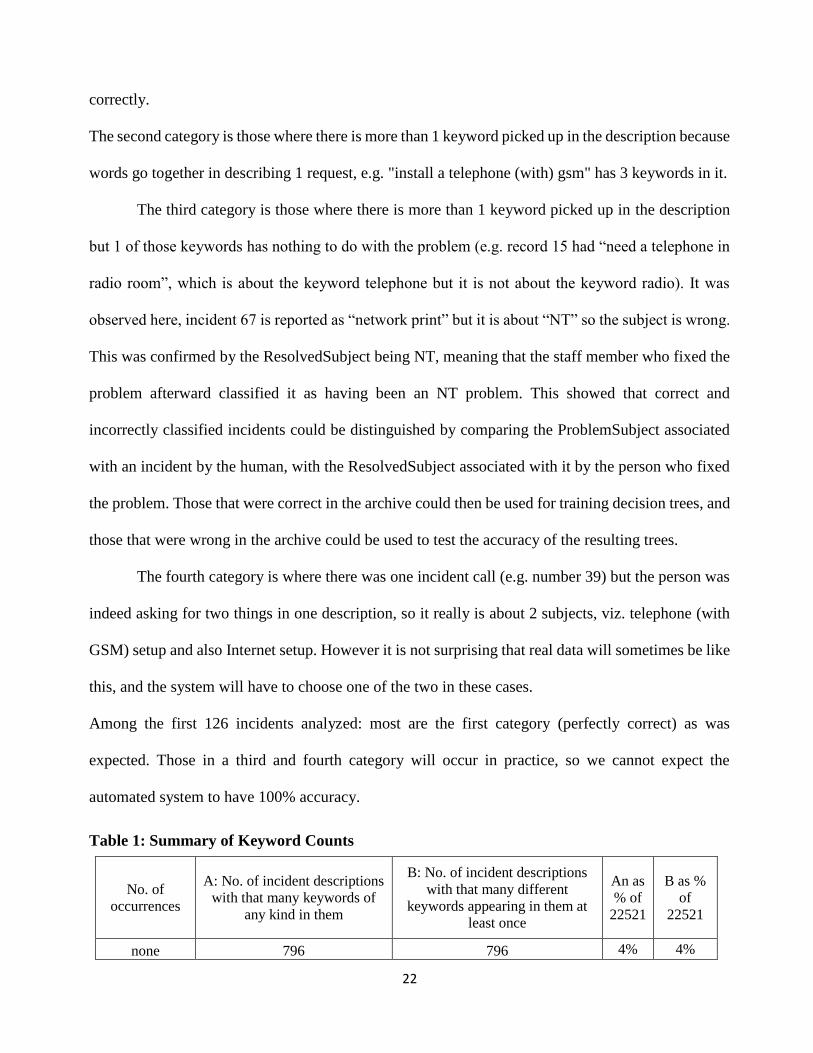
The second category is those where there is more than 1 keyword picked up in the description because
words go together in describing 1 request, e.g. "install a telephone (with) gsm" has 3 keywords in it.
The third category is those where there is more than 1 keyword picked up in the description
but 1 of those keywords has nothing to do with the problem (e.g. record 15 had “need a telephone in
radio room”, which is about the keyword telephone but it is not about the keyword radio). It was
observed here, incident 67 is reported as “network print” but it is about “NT” so the subject is wrong.
This was confirmed by the ResolvedSubject being NT, meaning that the staff member who fixed the
problem afterward classified it as having been an NT problem. This showed that correct and
incorrectly classified incidents could be distinguished by comparing the ProblemSubject associated
with an incident by the human, with the ResolvedSubject associated with it by the person who fixed
the problem. Those that were correct in the archive could then be used for training decision trees, and
those that were wrong in the archive could be used to test the accuracy of the resulting trees.
The fourth category is where there was one incident call (e.g. number 39) but the person was
indeed asking for two things in one description, so it really is about 2 subjects, viz. telephone (with
GSM) setup and also Internet setup. However it is not surprising that real data will sometimes be like
this, and the system will have to choose one of the two in these cases.
Among the first 126 incidents analyzed: most are the first category (perfectly correct) as was
expected. Those in a third and fourth category will occur in practice, so we cannot expect the
automated system to have 100% accuracy.
Table 1: Summary of Keyword Counts
No. of
occurrences
A: No. of incident descriptions
with that many keywords of
any kind in them
B: No. of incident descriptions
with that many different
keywords appearing in them at
least once
An as
% of
22521
B as %
of
22521
none 796 796 4% 4%

23
1 14773 15630 66% 69%
2 5078 4619 23% 21%
3 938 732 4% 3%
4 255 207 1% 1%
5 145 176 1% 1%
6 180 219 1% 1%
7 220 83 1% 0%
8 86 21 0% 0%
9 18 6 0% 0%
10 7 32 0% 0%
11 25 0 0% 0%
12 0 0 0% 0%
Table 1 shows how many keywords the incident descriptions typically contain. it can be see
that only 796 out of 22521 incidents, i.e. only 4% didn’t have any keywords in their description, the
rest have between 1 and 11 keyword occurrences. Often this is because the same keyword appears
over and over again in one description.
Column A is the counts of how many words in a description are one of the keywords; Column
B counts how many of the keywords are in a description. It is good to see here that 69% of the
descriptions use exactly one keyword so that will clearly indicate their subject. However quite a large
percentage, 21%, use 2 keywords. The decision tree will have to learn which of the 2 keywords to
use in assigning a Subject to these records. For example, it might be that the first keyword found is
the subject to assign. It is interesting to see that 32 incidents use as many as 10 different keywords!
Table 2: Summary of Subject Occurrences
Keyword
count Keyword
Subject
count Subject Subject/Keyword as %
899 Acrobat 618 Acrobat 69%
48 Power Pack 52 Power pack 108%
274 Battery 236 Battery 86%

24
45 Cartridge 35 Cartridge 78%
10 CD-ROM 8 CD-ROM 80%
148 Excel 133 Excel 90%
26 Fuser 19 Fuser Unit 73%
897 GSM 751 GSM 84%
68 HardDrive 74 Hard Drive 71%
537 Install 258 Install 48%
806 Internet 647 Internet 80%
226 Jam 138 Jam 61%
1590 Keyboard 1134 Keyboard 71%
209 Kitnomade 170 Kitnomade 81%
1050 laser 845 Printing 80%
6444 Lotus 6245 Lotus 97%
1098 Monitor 1437 Monitor 131%
909 Mouse 554 Mouse 61%
2616 Network 1873 Network 72%
456 NTaccount 1641 NT 541%
452 PDA 359 PDA 79%
48 PDF 22 PDF 46%
37 Printing 845 Printing 2113%
529 Profile 411 Profile 78%
550 Radio 336 Tetra Radio 61%
2021 Reset 846 Reset 42%
102 Sbox 64 Sbox 63%
778 Scan 478 Scan 61%
990 screen 1437 Monitor 145%
2 Smart Card 8 Smart 370%
599 SSO 126 SSO 21%
1168 Telephone 1039 Phone 89%
373 Tetra 336 Tetra Radio 83%
497 Toner 442 Toner 89%
191 T-Pass 190 T-PASS 99%
1374 VCR 1004 VCR 73%
76 Virus 28 virus 37%
195 Web mail 207 Web Mail 106%
.
The number of times each keyword appeared in the data was calculated, and the number of times
each Subject appeared in the data was also calculated. Excel was found to be sufficient to compute

25
and compare these counts, as shown in Table 2. If each incident used exactly one of the keywords,
namely the keyword associated with its Subject, then the count for each Subject would be equal to
the total counts of its associated keywords. Those where keyword and subject counts are very similar
are colored green and centered in the Comparison column. The percentages should generally be less
than 100% because a keyword can appear up to 11 times in one description, but each incident has
only 1 subject, so the number of appearances of that subject should be somewhat less than the number
of appearances of the keyword. Those colored blue and left-aligned are a little low indicating that this
keyword appears in descriptions where it is not the associated Subject, so the decision tree will have
to learn to detect those cases. Those colored amber and right-aligned are high percentages, indicating
that there are cases where some descriptions associated with a Subject did not contain the keyword;
the decision tree would have to learn how to handle these too.
Results of Subject Occurrences from the Table 2 showed keywords needed to be modified e.g. to
include a space. So, for example, the keyword "NT" was replaced by " NT" since otherwise it would
be wrongly counted as occurring when in fact it was only part of a word such as "iNTernet". Similarly,
the keyword “jam” was replaced by “jam ” to prevent user names containing this string, such as
“James”, from being counted as a keyword. An online tool [39] was used to see when a keyword can
be part of another word and in these cases, space was included in the keyword. Some keywords were
also shortened to detect all occurrences e.g. “smart” was used instead of “smart card” which can be
spelled as one word, two words or hyphenated. “CD” was used instead of “CD-ROM” and “Fuser”
instead of “Fuser unit” as these also improved the accuracy of keyword detection. Some keywords
such as “install” were shortened (e.g. to “install") because the data showed these were often
misspelled. These changes were made only in the Python program; the incident data was unchanged.

26
3.5 Implementation using WEKA Software
WEKA is referred to as open source software written using the object-oriented language
JAVA which is issued under the GNU general public license [41]. WEKA is a collection of tools for
data pre-processing, classification, regression, clustering, association and visualization [41]. Because
WEKA has a large collection of machine learning algorithms, it is widely used for exploring large
amounts of data [41]. Since the dataset we are using for this experiment has the same set of attributes
in every row, it is well suited to Attribute-Relation File Format (ARFF) which is the preferred method
for loading data in WEKA. The ARFF file defines each column and what each column contains and
then supplies the data itself. WEKA was used in three different ways:
First for machine learning using all database attributes, to see if it can learn from attribute
values that were kept as part of the archived data, exploring for example if particular kinds
of User Status were more likely to result in particular kind of Subject
Secondly, decision tree algorithms were used to train one model to predict incident Subject
using keywords in incident call descriptions
Thirdly for training a set of separate models, one to learn how to detect each subject based
on keywords in incident descriptions, in order to see if this would improve prediction
accuracy
3.5.1 Data loading in WEKA
The WEKA software is open source as stated above so it is very easy to download online, after
downloading the WEKA software, a start-up screen will pop-up. It contains four different options,
which are, Explorer, Experimenter, Knowledge Flow and simple CLI. However, in this work, we

27
make only use of the Explorer option because the functions in the other options were not applicable
to this work.
3.5.2 The Format for WEKA Files
The format of the file that is accepted to WEKA is Attribute Relation File Format (ARFF). The file
can be in ARFF or CSV format, which can be selected in the drop down list when loading the file in
WEKA. The file format is shown below.
@RELATION <name>. This is the name given to the dataset which will be loaded into WEKA.
@ATTRIBUTE
After that will be the list of all the attributes used as predictors, with their type. The attributes can be
Nominal values
Numerical values
String values
date and time
We considered only the numerical values because the features are counts (of how many times a
keyword appeared in the description) and only the Subjects are nominal values, where we need to list
all the possible values of Subject to be predicted.
Experience in this project showed that WEKA has very good error detection and any problem within
an ARFF file will result in a helpful message alerting one to the error and the line where it occurred.
@DATA

28
The data must be one row for each incident call, with commas to separate its attribute values. This
was produced by the Python program using its keyword counting function.
Another method of loading to WEKA is using CSV files. In this method, WEKA will select the CSV
file name as the relation. The attribute names will be taken from the first row of the CSV file and the
data will be the remaining content of the file.
The WEKA Input File
The ARFF file was created and loaded into the WEKA Explorer. The WEKA Explorer
includes a classified panel which enables a user to apply classification and regression algorithms [37]
[38] to the resulting dataset and helps to estimate the correctness of the resulting predictive model.

29
Figure 2: Sample of Input File to WEKA
Figure 3 shows Explorer with 35 attributes of keyword that was extracted from the incident
description of all incidents that had the correct subject assigned to them by the human operator.
Accuracy or incorrectness of Subject as assigned by the human operator was checked by comparing
it with the Subject subsequently assigned to that incident by the IT personnel after they had fixed
the problem (which was given in the archived data in a separate “ResolvedSubject” column).

30
Figure 4 Sample of 36 attributes loaded on WEKA Explorer.
In Figure 4 above, the Explorer display for easy review of the data input in WEKA is shown. The left
section of the display shows all the 36 attributes and the number of Instances. For Example, it can be
seen that 36 Attributes were added and 20,700 training instances extracted from the first incident

31
report. The attribute column (Subject) in the left part of the Explorer was selected, in the right section,
it shows the information about the data in that column of the given data set. However, the same thing
is applicable when any of the columns is selected. The numeric attributes show the Minimum,
Maximum, Mean and Standard deviation while nominal attributes show the possible values and the
number of times each value occurs. For example, the Subject was selected, its shows each Subject
that has been assigned to any particular incident description and how many times it occurred. It can
be seen that “Lotus” has the highest number of occurrences in which colors are used to differentiate
the Subjects.
3.5.3 Visualization of Input File
All columns can be visualized in order to examine the data at one glance. The data
visualization can be analyzed using different methods depending on the result to be achieved. A
different color is used to show occurrences of each ProblemSubject. This can be achieved by clicking
on the Visualize All button. Figure 5 below shows the result of doing so. Colours in this figure
correspond to the colours in figure 4.

32
Figure 5 Visualize All Data in a WEKA Explorer.
It can be seen that the X axis goes from 0 to 2 or 0 to5 etc because that is the range of values in that
column. For example, NumLotus goes from 0 to 2 because most Incident Descriptions had 0
occurrences of the word “Lotus”, but then some had 1 (or 2) because the word Lotus appeared in the
description once (or twice). The plot for any one attribute can be selected to show an enlarged plot
for that column. In the case of the keyword Lotus for example, where the count is 0 it can be seen

33
that the associated Subject varies widely, but where the count is 1 or 2 the associated Subject is almost
always “Lotus”.
CHAPTER 4
EXPERIMENTAL RESULTS
In this chapter, a comparative study of eight classification algorithms will be presented and
evaluated in terms of performance and accuracy. The dataset used for the experiment was obtained
from the Oil and Gas Company’s database which contained 22521 instances. The dataset contained
many fields including "ProblemSubject" and "ResolvedSubject". ResolvedSubject was the subject
given to the incident after the problem had been fixed.
4.1 Distinguishing Training and Test Data
The training dataset is given as input to the WEKA tool and various classification tools were
used. The input to the WEKA is an ARFF file containing the incident number, 35 integers
(representing word counts for each of the 35subject-keywords in turn) and the subject that was
assigned to that incident. Some incidents/records were used for training and the rest for checking
accuracy. After data cleaning had removed records with missing values using Excel, the data was
thus divided into 2 separate files: "ORIGINALLY-RIGHT" and "ORIGINALLY-WRONG" file. The
"ORIGINALLY-RIGHT" file was 20700 incidents which contained only cleaned, correct records.

34
This data set was then used for training WEKA. The "ORIGINALLY-WRONG" file contained the
remaining 1760 cleaned records, it was used to test if the tree learned by WEKA would classify these
incidents correctly or not.
The algorithm or procedures used for classification were J48, RandomTree, RandomForest,
REPTree, NBTree, LADTree, J48Graft, SimpleCart. Under the ‘Test options', the 10-fold cross-
validation was selected as our evaluation approach. Given that the evaluation data set is the same for
all 8 classifiers, it is possible to get a reasonable idea of the accuracy of the generated models. Each
model is generated in the form of a decision tree.Analyzing the classification performance of these
Decision Tree algorithms is supported by WEKA using a cross-validation approach. The performance
was compared in terms of correct/incorrect classified instances, time to build the model, Kappa
Statistic, Mean absolute error, etc. The purpose is to find the best algorithm to predict incident calls
Subject.
From the data analysis, it was found that some of the incidents were correctly entered in the
system while some were not correctly recorded due to human error. In the sample of 22522 incidents,
it was observed from the trained WEKA data that 1760 ProblemSubjects were different from the
ResolvedSubject.
Therefore the 20700 records with correct ProblemSubject were selected for the experiment; with all
the incorrect incidents (about 10 %) removed. These became the training and testing sets respectively.
4.1.1 Train and Test "ORIGINALLY-RIGHT" File

35
This file contained only those records where the ProblemSubject had been given correctly (i.e. was
the same as the ResolvedSubject) which is 20700 incidents. This data set was then used for training
WEKA.
The python code was used to produce an ARFF file with {incident number, number-of-Acrobat-
words-in-incident, number-of-Battery-words-in-incident, …, number-of-Virus-words-in-incident,
number-of-Webmail-words-in-incident, Subject} then it was input to WEKA for data classification
and decision trees training. The 35 numeric attributes were used to predict the final column i.e. the
Subject. The first attribute (Incident number) was not used for mining. This input was produced by
the python program that read in the incident descriptions one by one and created a comma-delimited
file with the keyword counts for each incident, followed by its Subject.
4.2 WEKA Model Training Results
The experiment used cross-validation because it takes a better approach by averaging over 10
different partitioning’s of the data set into training and test cases. The Model used is the Decision
Tree approach, although there are many other models in WEKA. Decision Tree was selected for this
dissertation because it can handle numerical data, and is a fast and understandable technique. The
experiment results are shown in Table 3 below.
Table 3. WEKA decision tree results using 10-fold cross-validation
Classifier
Kappa
Statistic
Mean
absolute
error
Root Mean
squared
error
Relative
absolute error
Root relative
squared error

36
J48 0.8875 0.0091 0.0681 18.0977 % 42.9748 %
Random Tree 0.8847 0.0081 0.0656 16.2397 % 41.4497 %
Random Forest 0.8851 0.0082 0.0651 16.2897 % 41.0908 %
REPTree 0.886 0.0088 0.0668 17.5967 % 42.1885 %
NBTree 0.8843 0.0087 0.0662 17.3115 % 41.8091 %
LAD Tree 0.7028 0.0218 0.099 43.3739 % 62.5309 %
J48Graft 0.8855 0.0091 0.0681 18.0974 % 42.9769 %
Simple Cart 0.8848 0.0085 0.066 16.8506 % 41.6673 %
Table 3 shows the results using 10-fold cross-validation for Classifiers Accuracy. Cross-
validation can be defined as a technique to evaluate predictive models by partitioning the original
sample into a training set to train the model, and a test set to evaluate it. With 10-fold cross-validation,
the data set is randomly divided into 10 equal-size subsets, and then 10 experiments are run, each one
using a different one of these subsets as the test set. Table 3 shows Kappa statistic, mean absolute
error, root mean squared error, relative absolute error percentage and root relative squared error
percentage. RandomForest has the lowest error rate; compared to LADTree which has the highest
error rate. The Kappa statistic can be defined as the chance-corrected measure of an agreement
between classifications and the true classes of a dataset. In the Kappa, a value of 0 means that the
classifier is equivalent to chance while a value of 1 means a perfect agreement of the classifier. Based
on the results shown, the Kappa rate of J48 is highest. Therefor J48 has highest predictive accuracy.
For the mean absolute error which measures the average magnitude of the errors in a set of forecasts,
the RandomForest algorithm has the lowest error rate to compared to the LADTree algorithm which
has the highest error rate - the smaller the error obtained, the better the result in terms of classification.

37
For the Root mean squared error which can be defined as the arithmetic means of the squares, the
LADTree has the worst root mean squared error while others are within the same range of root mean
squared error. Thus, among the eight classification algorithms that were investigated, J48 stood out
to be the best.
Table 4. Classifiers Accuracy of the incident description
Algorithm Percent Correctly classified
instances
Percent Incorrectly classified
instances
J48 89.985 10.015
Random Tree 89.9028 10.0972
Random Forest 89.9463 10.0537
REPTree 90.0285 9.9715
NBTree 89.8689 10.1311
LADTree 74.2997 25.7003
J48Graft 89.985 10.015
SimpleCart 89.9173 10.0827
Table 4 shows the accuracy of all the algorithms for the classification applied on the data sets using
10-fold cross validation. It can be seen that the highest accuracy is 90.0285 which REPTree and the
lowest accuracy is 74.2997 which is the LADTree. The next to the highest accuracy is 89.985 which
is the J48.
Table 5 shows the time in seconds taken by the various algorithms to build the model from
the training data.

38
The total time used to build the model is also an important parameter for algorithm comparison
classification. LADTree and NBTree have the longest model building time which are around 114.69
and 770.87 seconds followed by Random Forest which takes 23.14 seconds. It can be seen that J48
takes 0.04 seconds which is the shortest time to build the model. From all analyses, it can be seen that
J48 performs better than all other eight algorithms.
Table 5. The time takes to build a model for training data.
Algorithm Building time model in Seconds
J48 0.04
Random Tree 0.25
Random Forest 23.14
REPTree 0.78
NBTree 707.87
LADTree 114.69
J48Graft 2.51
SimpleCart 6.71
4.3 WEKA Test Result
The "ORIGINALLY-WRONG" file incidents were given the wrong subject by the human
operator and so those incidents were used for testing, not for training. The output training model from

39
J48 of the ORIGINALLY-RIGHT data was used to classify these new incidents. This is because J48
performed better than other algorithms as discussed in section 4.2 above. The subject was given as
"?" because then WEKA predicts the Subject using its tree that it has learned. In this process
"Supplied test set" was selected instead of “Cross-validation” in the Classify tab as shown in Figure
7. Comparison of this output with the ResolvedSubjects associated with these incidents showed 81%
of these predictions are correct, and moreover, the confidence level is correct too. Because where it
is 0.993 (99.3% confident in its prediction) it is indeed right – the Subject it has predicted is the same
as the ResolvedSubject for that incident in the archive. And where it is 0.87 (87% confident) it is
because the person asks for 2 things in one call e.g. keyboard and mouse replace, so it could indeed
classify the incident as either Keyboard or Mouse (it always chooses Keyboard). The values of the
Subjects that it automatically worked out for those incidents, based on the keywords appearing in
them and what it has learned previously (from the "ORIGINALLY-RIGHT" data training) about how
keyword counts map to Subject, made the system better than the human being who got those cases
wrong.
The test "ORIGINALLY-WRONG" file contained all 1760 records where the ProblemSubject
had been wrongly assigned as shown in Figure 6. This data was used to test if the tree learned by
WEKA would classify these incidents correctly or not. So under WEKA’s "Test options" instead of
selecting “cross validation”, the "Supplied test set" selection allows the system to predict Subjects for
the test instances. This is done by applying the generated model from the training stage, to the new
unclassified instances in the "ORIGINALLY-WRONG" file in order to predict the Subject value.

40

41
Figure 6: Sample of Input ORIGINALLY-WRONG File ARFF to WEKA

42
Figure 7 Test Set
The Table 6.which is the output from predicting subjects for records in the "ORIGINALLY-
WRONG" file does not show any accuracy statistics because the value of the class attribute was left
as "?", thus WEKA has no actual values to which it can compare the predicted values of new
instances.

43
Table 6: Predicted Result
Instance Actual Predicted Error Prediction
1 1:? 20: Mouse
0.993
2 1:? 20: Mouse
0.993
3 1:? 20: Mouse
0.993
4 1:? 13: Keyboa
0.87
5 1:? 20: Mouse
0.993
6 1:? 20: Mouse
0.993
7 1:? 20: Mouse
0.993
8 1:? 13: Keyboa
0.87
9 1:? 19: Monito
0.529
10 1:? 20: Mouse
0.993
11 1:? 20: Mouse
0.993
12 1:? 20: Mouse
0.993
- - - - - - - - - - - - - - -
1760 1:? 19: Monito 0.529
44
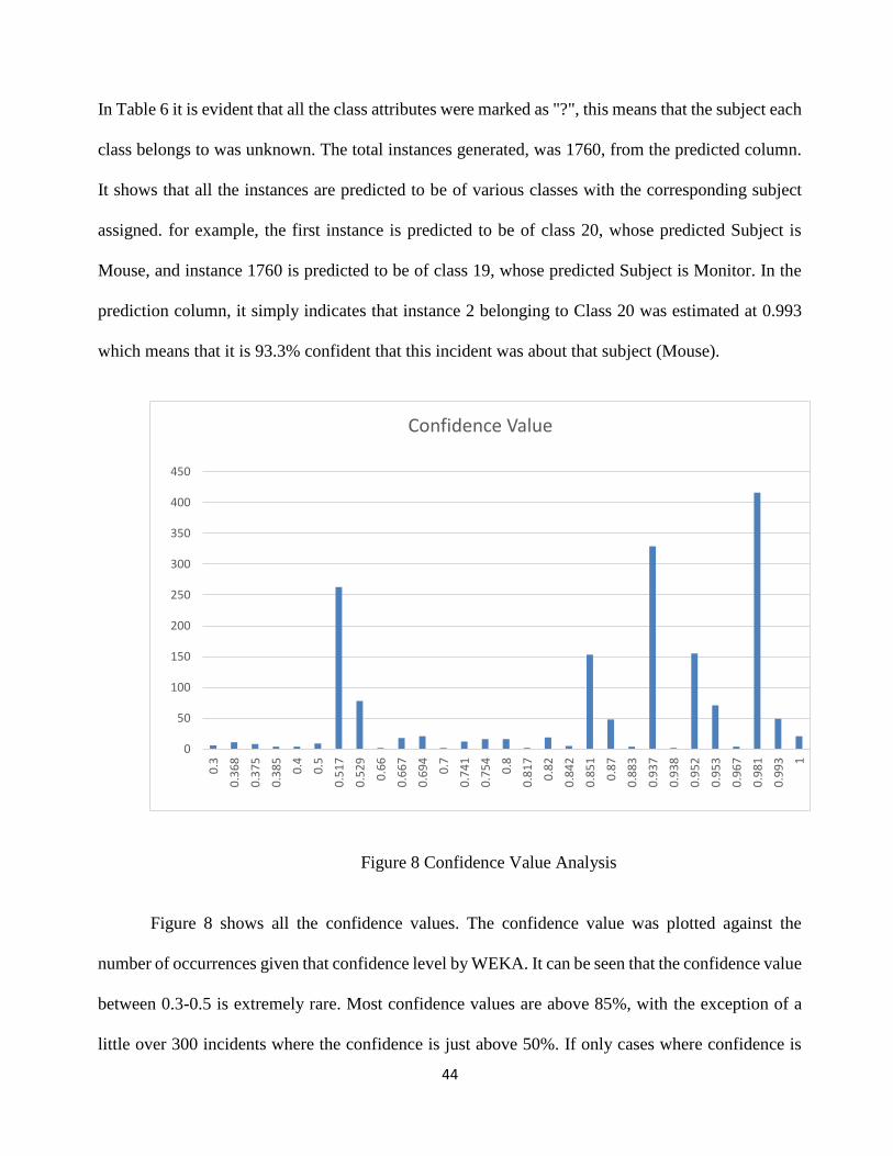
In Table 6 it is evident that all the class attributes were marked as "?", this means that the subject each
class belongs to was unknown. The total instances generated, was 1760, from the predicted column.
It shows that all the instances are predicted to be of various classes with the corresponding subject
assigned. for example, the first instance is predicted to be of class 20, whose predicted Subject is
Mouse, and instance 1760 is predicted to be of class 19, whose predicted Subject is Monitor. In the
prediction column, it simply indicates that instance 2 belonging to Class 20 was estimated at 0.993
which means that it is 93.3% confident that this incident was about that subject (Mouse).
Figure 8 Confidence Value Analysis
Figure 8 shows all the confidence values. The confidence value was plotted against the
number of occurrences given that confidence level by WEKA. It can be seen that the confidence value
between 0.3-0.5 is extremely rare. Most confidence values are above 85%, with the exception of a
little over 300 incidents where the confidence is just above 50%. If only cases where confidence is
0
50
100
150
200
250
300
350
400
450
0.3
0.3
68
0.3
75
0.3
85
0.4
0.5
0.5
17
0.5
29
0.6
6
0.6
67
0.6
94
0.7
0.7
41
0.7
54
0.8
0.8
17
0.8
2
0.8
42
0.8
51
0.8
7
0.8
83
0.9
37
0.9
38
0.9
52
0.9
53
0.9
67
0.9
81
0.9
93 1
Confidence Value

45
below 85% are given to the human operator; this should then reduce his/her work by more than 80
percent.
Table 7: System Confidence Levels
ProblemSubject Average confidence level Range of confidence levels
WEKA Wrongly Assigned 0.8 from 0.333 to 1
WEKA Correctly Assigned 0.9
from 0.333 to 1
From Table 7 it can be seen that the average confidence level with which WEKA predicted subjects when it
was incorrect was 80%; while the average confidence level with which WEKA predicted subjects correctly
was 92%. In both the correct and the incorrect classifications, individual predictions had confidence levels
ranging from 33% to 100% confident.
Table 8: System Performance
ProblemSubject Percentage
Total WEKA got RIGHT 81%
Total WEKA got WRONG 19%
Table 8 shows WEKA correctly classified 81% of the test cases that had been wrongly classified by
humans. It wrongly classified 19% of them, usually because of more than one problem in one incident
call

46
4.4 Second Approach using Decision Tree
The way the decision trees were used was compared with an alternative approach using
separate decision trees to recognize each Subject. Two Subjects were selected for the experiment
(Lotus and Mouse) because these occurred most frequently in both the ORIGINALLY-RIGHT and
ORIGINALLY-WRONG files. For the Mouse case, the decision trees in WEKA had to learn to
predict "Mouse" or "not Mouse". This experiment was done - to see if it does this more accurately
than it did when predicting "Mouse" with the tree obtained with the previous approach. In the new
copy of the input, all the training data had Subject replaced by "no" except where it was "Mouse",
which was kept unchanged as the Subject in those rows. The same was done with the “Lotus”
experiment. Figure 9 and 10 below shows the result of the decision tree analysis;

47
Figure 9 Alternative Approach: Decision Tree for Mouse

48
Figure 10 Alternative Approach: Decision Tree for Lotus
It is interesting to see the structure of the decision tree. The model accuracy predicted both
Mouse and Lotus as expected in terms of how No was mapped out and that of Yes too. Some paths
do have two or three tests, like numMouse and numKeyword in the decision tree for Mouse cases.
The model predicted it the same way when all the Subjects are together.

49
Table 9: Time taken to build a model using the second approach
Algorithm Building time model in Seconds
J48 1.62
Random Tree 0.21
Random Forest 1.42
REPTree 0.51
NBTree 2.81
LADTree 3.47
J48Graft 1.23
SimpleCart 2.02
The table above shows the speed of each algorithm i.e. how long they took on these 1760
cases. From the Table above, LADTree has the longest model building time which is around 3.47
seconds followed by NBTree which is 2.81.
4.5 Test Results of Second Approach
The two solutions (models) were run against the test-data used for evaluating the work in the
dissertation so far, however, this was done to see how good it is at picking up Mouse and Lotus on
those cases that the human had done wrong. Two tests were run, one using the new tree/model for
Mouse to see how good it is on the test data set for detecting Mouse, and then afterward using the
new tree/model for Lotus to see how good it is on the test data set for detecting Lotus cases. The
results, some of which are shown in Table 10, were much worse than with the first approach.

50
Table 10: Predicted Result for Test Cases using Second Approach
inst# actual predicted error prediction 1 1:? 45:No 0.987
38 1:? 16:Lotus 0.999
59 1:? 16:Lotus 0.611
82 1:? 45:No 1
83 1:? 45:No 1
89 1:? 45:No 1
94 1:? 45:No 1
111 1:? 16:Lotus 0.999
112 1:? 16:Lotus 0.999
164 1:? 45:No 1
165 1:? 45:No 1
196 1:? 45:No 1
197 1:? 45:No 1
200 1:? 45:No 1
201 1:? 45:No 1
204 1:? 45:No 1
205 1:? 45:No 1
246 1:? 16:Lotus 0.999
247 1:? 16:Lotus 0.999
284 1:? 16:Lotus 0.999
285 1:? 16:Lotus 0.999
414 1:? 16:Lotus 0.999
415 1:? 16:Lotus 0.999
416 1:? 16:Lotus 0.999
417 1:? 16:Lotus 0.999
1526 1:? 16:Lotus 0.611
The above table shows a sample of output produced, where all output lines omitted were the same
as the first line i.e. they all predicted “No” with 98.7% confidence. This time the prediction was very poor. It
picked up very few of the Lotus cases indeed and even predicted that a Lotus row is a "No" with a

51
confidence of 1 (i.e. completely confident) when actually that row was indeed a "Lotus" problem.
The alternative approach of using separate decision trees for each Subject was thus not studied
further.
CHAPTER 5
CONCLUSION
In this chapter, the experimental results will be evaluated to conclude the comparison of the
different algorithms and the discussion of the proposed framework. This chapter also suggests ways
improve the system and proposes further work for the research.
5.1 Conclusion
This dissertation proposed an analysis of IT incident calls using data from an African oil and
gas company as a case study. Nowadays, much time is being spent at this company to resolve the
issue of wrongly assigned subjects for IT incident calls. In this dissertation, an approach was
developed in other to tackle the problem of assigning a subject to these incident calls. The proposed
framework will help by classifying the subject of an incident description using counts of specific

52
keywords and classification algorithms produced using WEKA software. The aim was to determine
the best algorithm as well as its speed and accuracy. The trained model will analyze the incident
description and predict the possible subject to handle the incident. All this involves data preparation,
method selection, and data exploration.
Research Questions
Each of the research questions of this work is addressed here.
Question 1: Can an automated system assign a subject to OGA calls with acceptable accuracy?
The first objective of this research aims to use an automated system to assign a subject to OGA calls
with acceptable accuracy. Experimental results using 10-fold cross validation in WEKA showed that,
except for the LADTree, all decision trees achieved 90% accuracy. In comparison, human operators
achieved 92% accuracy (20700 were correct out of 22460). This is thus acceptable accuracy, and
moreover, has the speed and cost benefits of automation.
Question 2: Can this assign correct subjects to those OGA calls where humans were incorrect?
Archived data was first split into two files. The "ORIGINALLY-RIGHT" file, which contained only
records where the Problem Subject had been given correctly, was used for training and the
"ORIGINALLY-WRONG" file, which contained records where the Problem Subject had been
wrongly assigned, was used to test if the tree learned by WEKA would classify these incidents
correctly. From the experimental results, this proved to be more effective than a human assignment
of subjects at OGA, as 81% of incidents wrongly classified by humans were correctly classified by
the system. A keyword-based approach is thus recommended for decision tree classifying of IT
incident calls.
One of the problems with a keyword-based approach to data mining is that you have so many

53
attributes and most mining methods cannot deal well with so many attributes. However, In this
dissertation, we were able to analyze and summarize the data into 35 attributes. The proposed model
will be helpful not only for the OGA IT helpdesk staff but can also be adapted to analyze any
keyword-based approach to classification in other studies.
Question 3: Which decision tree algorithm is best for this in terms of accuracy and
performance? In the decision tree comparison using WEKA software, the J48 method had the
highest predictive accuracy and was a better method when compared with eight other WEKA
decision tree algorithms. Based on the results obtained in this dissertation, the J48 has the Kappa
rate of 0.8875 which is the highest of all. It also has the highest percentage of predictive
accuracy. While it does not have the lowest mean absolute error nor the lowest Root Mean
squared error, these values for J48 are only slightly above the minimum found. The experimental
results indicate that the J48 takes 0.04 seconds which is the shortest time to build the model. The
short period indicates that J48 will produce the fastest solution in resolving IT incident call
Subjects.
Thus this WEKA decision tree can now be used in a recommendation system to predict
the Subject of IT incidents in real world applications.
5.2 Future work
Although we have used WEKA decision trees in the above predictions, we also envisage that
theoretically the same problem can be handled using Support Vector Machines (SVM) (based on
many to one voting) or Multinomial Logistic Regression (MLR).In future, it would be of interest

54
to consider other machine learning algorithms and compare the result with decision trees.
Furthermore, a system is needed that will incorporate all the processing, including the newly
developed model linking directly to the incoming incident calls so that once an issue is assigned it
will automatically send a mail to the personnel that will resolve the incident with all the details
required. The system can also be linked to a knowledge database which will assist in resolving
future incidents based on how similar problems were solved.

55
References
1. K Giberta, M. Sànchez-Marrèa and B. Sevilla. Tools for Environmental Data Mining and Intelligent
Decision Support, International Congress on Environmental Modelling and Software, 2012.
2. C. Carrier and O. Povel. Characterizing Data Mining software, Intelligent Data Analysis, Vol. 7 No. 3, pp
181-192, August 2003.
3. WEKA Data Mining tool. www.cs.waikato.ac.nz/~ml/WEKA, last accessed May 2014.
4. A. H. Wahbeh, Q. A. Al-Radaideh, M. N. Al-Kabi and E M. Al-Shawakfa. A Comparison Study between
Data Mining Tools over some Classification Methods, (IJACSA) International Journal of Advanced Computer
Science and Applications, Special Issue on Artificial Intelligence, pp 18-26, 2012.
5. M. J. ArtiTyagi. Data Mining: A Prediction for Performance Improvement in on line Learning Systems
International Journal of Advanced Research in Computer Science and Software Engineering, Vol. 3 No. 7,
July 2013.
6. J. Han and M. Kamber. Data Mining: Concepts and Techniques, 2nd ed., Morgan Kaufmann, New York,
Elsevier, 2009.
7. T.M Mitchell. Machine Learning, McGraw-Hill, 1997.
8. J R Quinlan. Induction of Decision Trees, Machine Learning, Vol. 1, pp 81-106, 1986.
9. J. Han and M. Kamber. Data Mining Concepts and Techniques, 2nd ed., Morgan Kaufmann, San Francisco,
CA, 2007.
10. M. H. Dunham. Data Mining Introductory and Advanced Topics, Pearson Education (Singapore), Delhi,
India, 2004.
11. J R Quinlan. C4.5: Programs for Machine Learning, Morgan Kaufmann, San Mateo, CA, 1993.
12. R. O.Duda, P. E Hart and D. Stork. Pattern classification, 2nd ed., John Wiley & Sons, New York NY,
2001.
13. L. Breiman, J. H. Friedman, R. A. Olshen and P. J. Stone. Classification and regressing trees, Wadsworth
International, 1984.
14. R.J. Lewis. An Introduction to Classification and Regression Tree (CART) Analysis, 2000 Annual Meeting
of the Society for Academic Emergency Medicine, Francisco, California, 2000.
15. R. W. Yeung. Information Theory and Network Coding, Springer, 2008.
16. Kullback, S. Letter to the Editor: The Kullback – Leibler distance, The American Statistician, Vol. 41 No.
4, pp.340-341, 1987.
17. R. Kohavi. A Study of Cross-Validation and Bootstrap for Accuracy Estimation and Model Selection,
Proceedings of the 14th International Joint Conference on Artificial Intelligence, Vol. 2, pp 1137–1143,

56
Morgan Kaufmann, USA, 1995.
18. L. Breiman. Random Forests.Springer, Machine Learning, Vol. 45 No. 1, pp 5-32, 2001.
19. I. Witten and E. Frank. Data Mining: Practical Machine Learning Tools and Techniques with Java
Implementations. 2nd ed., San Mateo, California, Morgan Kaufmann, 2005.
20. A. K. Sharma and S. Sahni. A Comparative Study of Classification Algorithms for Spam Email Data
Analysis, International Journal on Computer Science and Engineering (IJCSE), Vol.3. No. 5, May 2011.
21. A. H. M. Ragab, A. Y. Noaman, A. S. Al-Ghamdi and A. I. Madbouly. A Comparative Analysis of
Classification Algorithms for Students College Enrollment Approval Using Data Mining, Proceedings of the
2014 Workshop on Interaction Design in Educational Environments (IDEE ’14), Eds. H. M. Fardoun and J.
A. Gallud, ACM, 2014.
22. T. M. Lakshmi, A. Martin, R. M. Begum and V. P. Venkatesan. An Analysis on Performance of Decision
Tree Algorithms using Student’s Qualitative Data, International Journal of Modern Education and Computer
Science (IJMECS), Vol. 5 No. 5, pp 18-27, June 2013.
23. S. Khatwani and A. Arya. A Novel Framework for Envisaging a Learner's Performance using Decision
Trees and Genetic Algorithm, Proceedings of the 2013 International Conference on Computer Communication
and Informatics (ICCCI), India, IEEE, 2013.
24. J-J. Wang, J-F. Wang, F. Lu, Z-D. Cao, Y-L. Liao and Y. Deng. Comparison Study on Classification
Performance for Short-Term Urban Traffic Flow Condition Using Decision Tree Algorithms, Proceedings of
the WRI World Congress on Software Engineering (WCSE '09), Vol. 4, pp 434 – 438, IEEE, 2009.
25. S. K. Yadav and S. Pal. Data Mining: A Prediction for Performance Improvement of Engineering Students
using Classification, World of Computer Science and Information Technology Journal (WCSIT), Vol. 2 No.
2, pp 51-56, 2012.
26. B Hssina, A. Merbouha, H. Ezzikouri and M. Erritali. A comparative study of decision tree ID3 and C4.5,
International Journal of Advanced Computer Science and Applications, Special Issue on Advances in
Vehicular Ad Hoc Networking and Applications, www.ijacsa.thesai.org
27. R. Sathya and A. Abraham. Comparison of supervised and unsupervised learning algorithm for pattern
classification, International Journal of Advanced Research in Artificial Intelligence, Vol. 2 No 2, 2013.
28. J. J. Hopfield. Neural Networks and Physical Systems with Emergent Collective Computational Abilities,
Proceedings of the National Academy of Science of the USA, Vol.79 No.8, pp 2554-2558, April 1982.
29. C. A. Gail and G. B Stephen. Adaptive resonance theory, Encyclopedia of Machine Learning, CAS/CNS
Technical report, May 2009.
30. A. Oludele and J. Olawale. Neural network and its Application in Engineering, Proceedings of Information
Science and IT Education Conference, 2009.
31. K. Andrej, B. Janez and K. Andrej. Introduction to the artificial neural networks,
32. NASA Ames Research Centre. Introduction to IND Version 2.1. GA23-2475-02 ed.. 1992.

57
33. J. R. Quinlan and R. L. Rivest. Inferring Decision Trees using Minimum Description Length Principle,
Information and Computation, Vol. 80 No. 3, pp 227 – 248, Academic Press, USA, 1989.
34. WEKA 3 - Data Mining with open source machine learning software. Available from
http://www.cs.waikato. ac.nz/ml/WEKA/, last accessed September 2017.
35. G. Holmes, A. Donkin and I. H. Witten. WEKA a machine learning workbench. In: Proceedings 2nd
Australia and New Zealand Conference on Intelligent Information System, Brisbane, Australia, pp.357-361,
1994.
36. S.-G. P. V. Purdila. Fast decision tree algorithm, Advances in Electrical and Computer Engineering, Vol.
14 No. 1, pp 65 – 68, 2014.
37. E. Frank, M. Hall, G. Holmes, R. Kirkby, B. Pfahringer, I. H. Witten and L. Trigg. WEKA, Data Mining
and Knowledge Discovery Handbook, Springer, pp. 1305–1314, 2005.
38. M. Hall, E. Frank, G. Holmes, B. Pfahringer, P. Reutemann and I. H. Witten. The WEKA Data Mining
Software: an Update, ACM SIGKDD Explor. Newsletter, Vol. 11 No. 1, pp. 10–18, 2009.
39. http://www.litscape.com/word_tools/contains_sequence.php
40. D. Alao. & A. B. Adeyemo. Analyzing Employee Attrition Using Decision Tree Algorithms, Computing,
Information Systems & Development Informatics, Vol. 4 No. 1, pp 17-28, March, 2013.
41. R. Bouckaert, E. Frank, M. Hall, G. Holmes, B. Pfahringer, P. Reutemanm and I. Witten. WEKA -
Experience with a Java Open-Source, Journal of Machine Learning Research, Vol. 11, 2533-2541, 2010.
42. J.R. Quinlan. Induction of Decision Trees, Centre for Advanced Computing Sciences, New South Wales
Institute of Technology, Sydney Australia, 2007.
43. S. Agarwal, G. N. Pandey and M. D. Tiwari. Data Mining in Education: Data Classification and Decision
Tree Approach, International Journal of e-Education, e-Business, e-Management and e-Learning, Vol. 2 No.
2, April 2012.
44. ENISA Work Programme 2010. http://www.enisa.europa.eu/media/key-documents/enisa-work-
programme-2010
45. B. R Patel and K. K. Rana. A Survey on Decision Tree Algorithms for Classification, IJEDR Vol. 2
No. 1, ISSN: 2321-9939, 2014.
46. P. Tan, M. Steinbach and V. Kumar. Introduction to Data Mining, Addison-Wesley, 2006.
47. A. Ashari, I. Paryudi and A. M. Tjoa. Performance Comparison between Naïve Bayes, Decision Tree
and k-Nearest Neighbor in Searching Alternative Design in an Energy Simulation Tool, International Journal
of Advanced Computer Science and Applications (IJACSA), Vol. 4,No. 11, 2013.
48 G. Holmes, B. Pfahringer, R. Kirkby, E. Frank and M. Hall. Multiclass Alternating Decision Trees,
http://www.cs.waikato.ac.nz/~bernhard/papers/ecml2002.pdf, 2002.
49. J. Ali, R. Khan, N. Ahmad and I. Maqsood. Random Forests and Decision Trees, IJCSI International

58
Journal of Computer Science Issues, Vol. 9 No 3, September 2012.
50. M. Cernak. A Comparison of Decision Tree Classifiers for Automatic Diagnosis of Speech Recognition
Errors, Computing and Informatics, Vol. 29, pp 1001–1013, 2010.
51. R. Revathy and R. Lawrance. Comparative Analysis of C4.5 and C5.0 Algorithms on Crop Pest Data,
International Journal of Innovative Research in Computer and Communication Engineering, Vol. 5, Special
Issue 1, March 2017.
52 L. Devasena. C Comparative Analysis of Random Forest, REP Tree and J48 Classifiers for Credit Risk
Prediction, International Journal of Computer Applications (0975 – 8887) International Conference on
Communication, Computing and Information Technology (ICCCMIT), 2014.
53. A.Lazarov and P. Shoval. A Rule-based System for Automatic Assignment of Technicians to Service
Faults, Decision Support Systems, Vol. 32, pp 343-360, Elsevier, 2002