Embed Size (px)
Citation preview

Decision Procedures in Verification
Decision Procedures (3)
19.12.2013
Viorica Sofronie-Stokkermans
e-mail: [email protected]
1

Until now:
Decidable subclasses of FOL
The Bernays-Schonfinkel class
(definition; decidability;tractable fragment: Horn clauses)
The Ackermann class
The monadic class
Decision problems/restrictions
Uninterpreted function symbols
Decision procedures for numeric domains
Difference logic
2
Positive difference logic
Syntax
The syntax of formulae in positive difference logic is defined as follows:
• Atomic formulae (also called difference constraints) are of the form:
x − y ≤ c
where x , y are variables and c is a numerical constant.
• The set of formulae is:
F ,G ,H ::= A (atomic formula)
| (F ∧ G) (conjunction)
Semantics:
Versions of difference logic exist, where the standard interpretation is Q or
resp. Z.
3

Positive difference logic
A decision procedure for positive difference logic (≤ only)
Let S be a set (i.e. conjunction) of atoms in (positive) difference logic.
G(S) = (V ,E ,w), the inequality graph of S , is a weighted graph with:
• V = X (S), the set of variables occurring in S
• e = (x , y) ∈ E with w(e) = c iff x − y ≤ c ∈ S
Theorem 3.4.1.
Let S be a conjunction of difference constraints, and G(S) the inequality
graph of S . Then S is satisfiable iff there is no negative cycle in G(S).
Searching for negative cycles in a graph can be done with the Bellman-Ford
algorithm for finding the single-source shortest paths in a directed weighted
graph in time O(|V | · |E |). (Side-effect of the algorithm exploited - if there
exists a negative cycle in the graph then the algorithm finds it and aborts.)
4
Positive difference logic
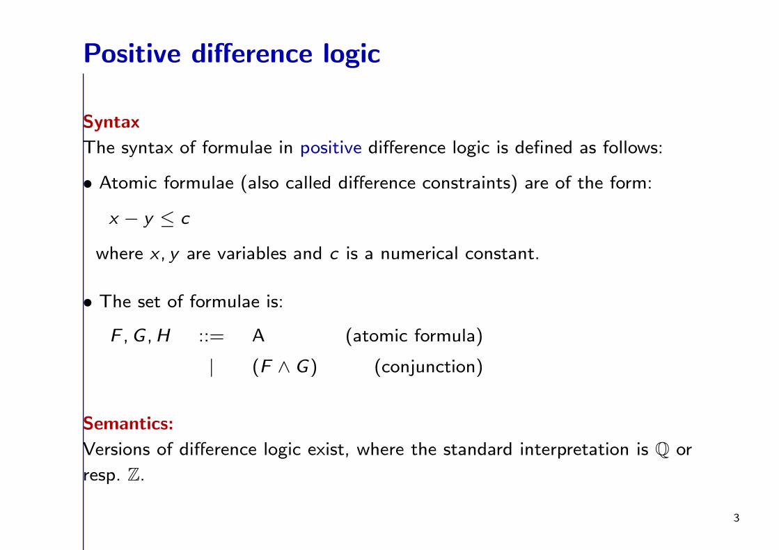
Theorem 3.4.1.
Let S be a conjunction of difference constraints, and G(S) the inequality
graph of S . Then S is satisfiable iff there is no negative cycle in G(S).
Proof: (⇒) Assume S satisfiable. Let β : X → Z satisfying assignment.
Let v1c12→ v2
c23→ · · ·cn−1,n→ vn
cn1→ v1 be a cycle in G(S).
Then: β(v1)− β(v2) ≤ c12
β(v2)− β(v3) ≤ c23
. . .
g β(vn)− β(v1) ≤ cn1
0 = β(v1)− β(v1) ≤∑n−1
i=1 ci ,i+1 + cn1
Thus, for satisfiability it is necessary that all cycles are positive.
5
Positive difference logic
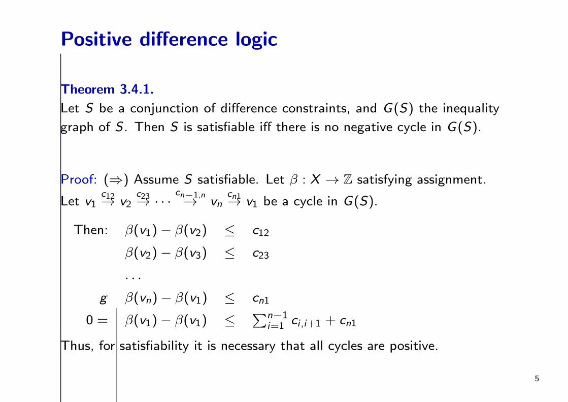
Theorem 3.4.1.
Let S be a conjunction of difference constraints, and G(S) the inequality
graph of S . Then S is satisfiable iff there is no negative cycle in G(S).
Proof: (⇐) Assume that there is no negative cycle.
Add a new vertex s and an 0-weighted edge from every vertex in V to s.
(This does not introduce negative cycles.)
Let δuv denote the minimal weight of the paths from u to v .
• δuv = ∞ if there is no path from u to v .
• well-defined since there are no negative cycles
Define β : V → Z by β(v) = δvs . Claim: β satisfying assignment for S .
Let x − y ≤ c ∈ S . Consider the shortest paths from x to s and from y to
s. By the triangle inequality, δxs ≤ c + δys , i.e. β(x)− β(y) ≤ c.
6
Difference logic
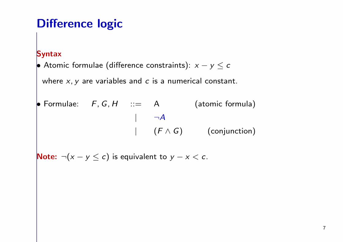
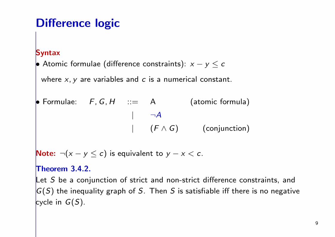
Syntax
• Atomic formulae (difference constraints): x − y ≤ c
where x , y are variables and c is a numerical constant.
• Formulae: F ,G ,H ::= A (atomic formula)
| ¬A
| (F ∧ G) (conjunction)
Note: ¬(x − y ≤ c) is equivalent to y − x < c.
7

Difference logic
Syntax
• Atomic formulae (difference constraints): x − y ≤ c
where x , y are variables and c is a numerical constant.
• Formulae: F ,G ,H ::= A (atomic formula)
| ¬A
| (F ∧ G) (conjunction)
Note: ¬(x − y ≤ c) is equivalent to y − x < c.
Satisfiability over Z
y − x < c iff y − x ≤ c − 1
Natural reduction to positive difference logic.
8
Difference logic
Syntax
• Atomic formulae (difference constraints): x − y ≤ c
where x , y are variables and c is a numerical constant.
• Formulae: F ,G ,H ::= A (atomic formula)
| ¬A
| (F ∧ G) (conjunction)
Note: ¬(x − y ≤ c) is equivalent to y − x < c.
Theorem 3.4.2.
Let S be a conjunction of strict and non-strict difference constraints, and
G(S) the inequality graph of S . Then S is satisfiable iff there is no negative
cycle in G(S).
9
Difference logic
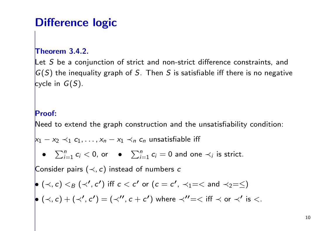
Theorem 3.4.2.
Let S be a conjunction of strict and non-strict difference constraints, and
G(S) the inequality graph of S . Then S is satisfiable iff there is no negative
cycle in G(S).
Proof:
Need to extend the graph construction and the unsatisfiability condition:
x1 − x2 ≺1 c1, . . . , xn − x1 ≺n cn unsatisfiable iff
•∑n
i=1 ci < 0, or •∑n
i=1 ci = 0 and one ≺i is strict.
Consider pairs (≺, c) instead of numbers c
• (≺, c) <B (≺′, c′) iff c < c′ or (c = c′, ≺1=< and ≺2=≤)
• (≺, c) + (≺′, c′) = (≺′′, c + c′) where ≺′′=< iff ≺ or ≺′ is <.
10
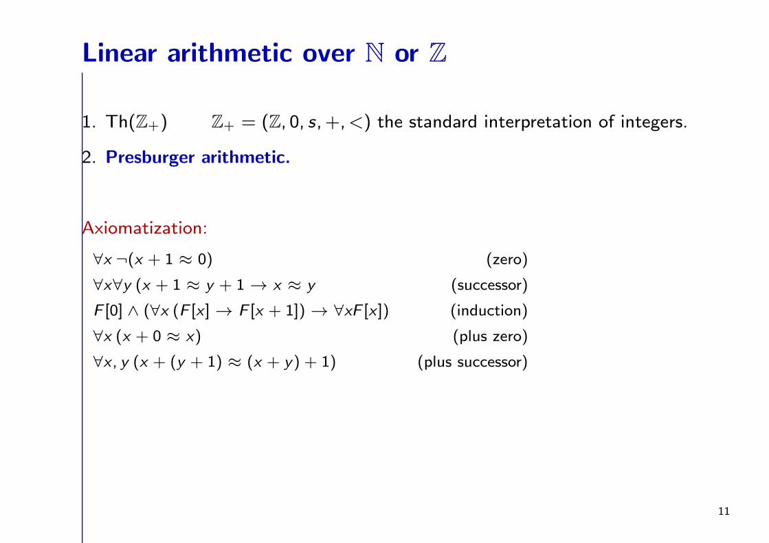
Linear arithmetic over N or Z
1. Th(Z+) Z+ = (Z, 0, s, +,<) the standard interpretation of integers.
2. Presburger arithmetic.
Axiomatization:
∀x ¬(x + 1 ≈ 0) (zero)
∀x∀y (x + 1 ≈ y + 1 → x ≈ y (successor)
F [0] ∧ (∀x (F [x] → F [x + 1]) → ∀xF [x]) (induction)
∀x (x + 0 ≈ x) (plus zero)
∀x , y (x + (y + 1) ≈ (x + y) + 1) (plus successor)
11
Linear arithmetic over N or Z
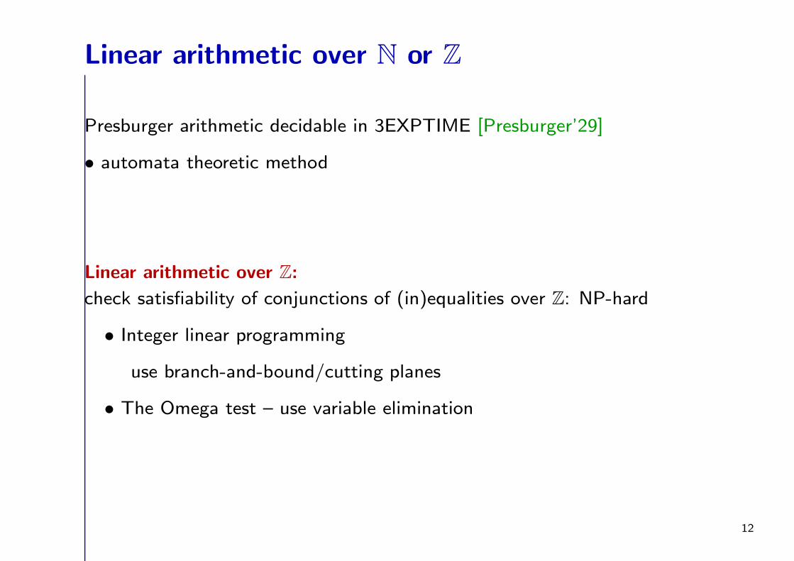
Presburger arithmetic decidable in 3EXPTIME [Presburger’29]
• automata theoretic method
Linear arithmetic over Z:
check satisfiability of conjunctions of (in)equalities over Z: NP-hard
• Integer linear programming
use branch-and-bound/cutting planes
• The Omega test – use variable elimination
12
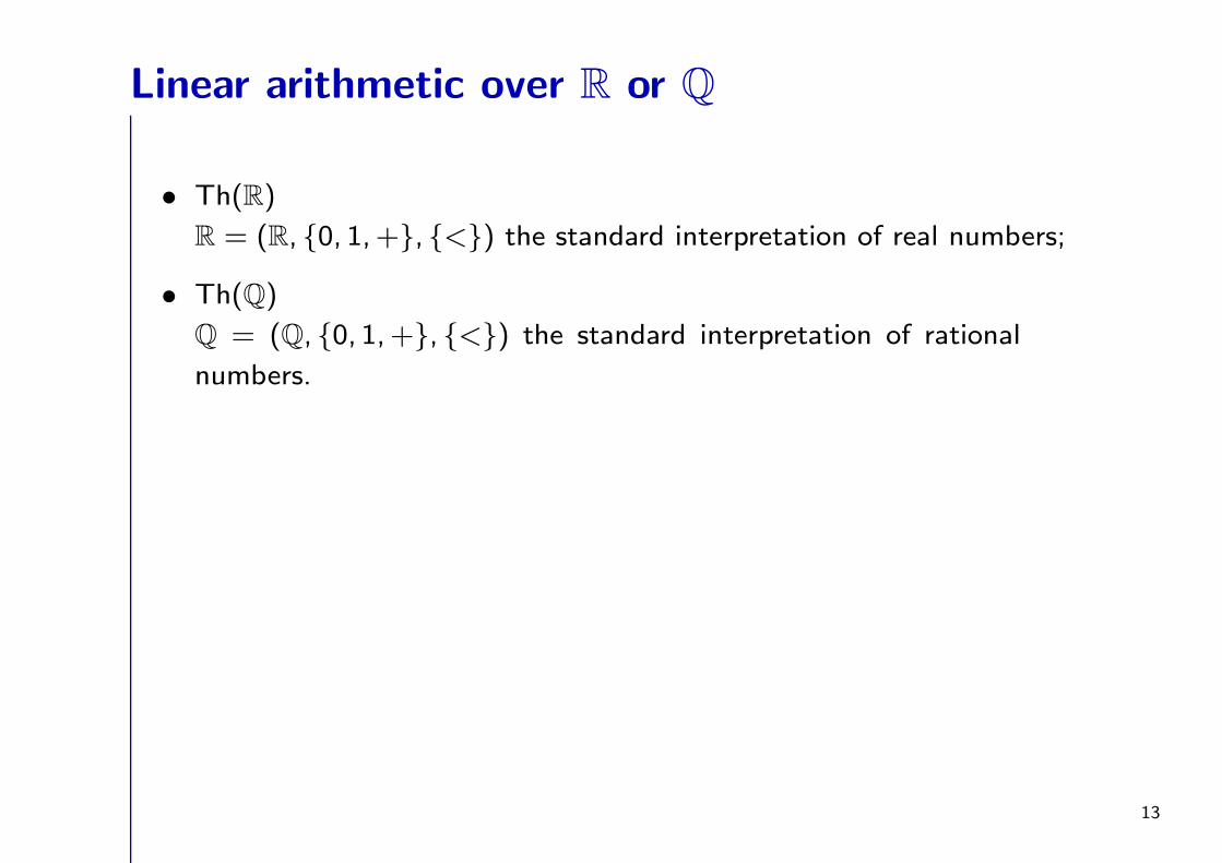
Linear arithmetic over R or Q
• Th(R)
R = (R, 0, 1,+, <) the standard interpretation of real numbers;
• Th(Q)
Q = (Q, 0, 1,+, <) the standard interpretation of rational
numbers.
13
Linear arithmetic over R or Q
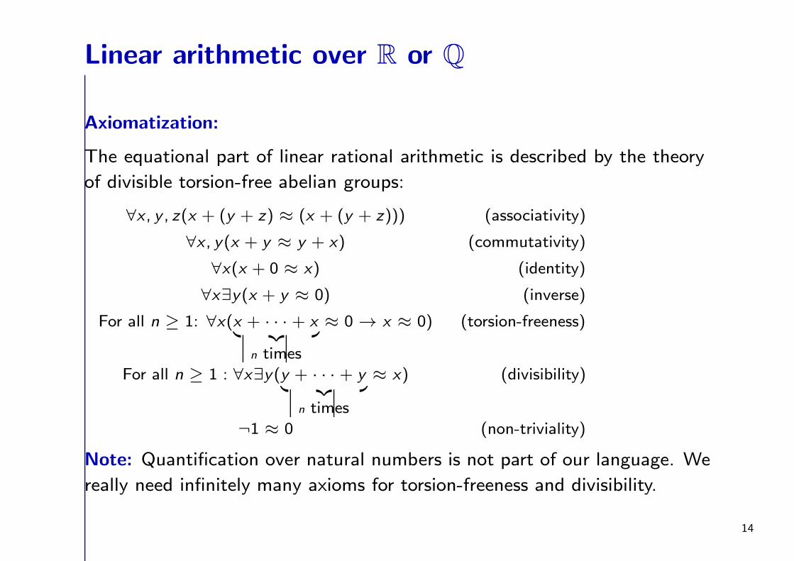
Axiomatization:
The equational part of linear rational arithmetic is described by the theory
of divisible torsion-free abelian groups:
∀x , y , z(x + (y + z) ≈ (x + (y + z))) (associativity)
∀x , y(x + y ≈ y + x) (commutativity)
∀x(x + 0 ≈ x) (identity)
∀x∃y(x + y ≈ 0) (inverse)
For all n ≥ 1: ∀x(x + · · · + x︸ ︷︷ ︸
n times
≈ 0 → x ≈ 0) (torsion-freeness)
For all n ≥ 1 : ∀x∃y(y + · · · + y︸ ︷︷ ︸
n times
≈ x) (divisibility)
¬1 ≈ 0 (non-triviality)
Note: Quantification over natural numbers is not part of our language. We
really need infinitely many axioms for torsion-freeness and divisibility.
14
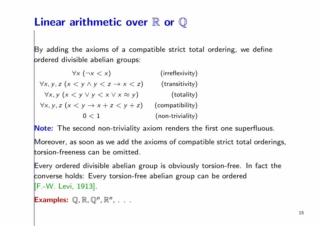
Linear arithmetic over R or Q
By adding the axioms of a compatible strict total ordering, we define
ordered divisible abelian groups:
∀x (¬x < x) (irreflexivity)
∀x , y , z (x < y ∧ y < z → x < z) (transitivity)
∀x , y (x < y ∨ y < x ∨ x ≈ y) (totality)
∀x , y , z (x < y → x + z < y + z) (compatibility)
0 < 1 (non-triviality)
Note: The second non-triviality axiom renders the first one superfluous.
Moreover, as soon as we add the axioms of compatible strict total orderings,
torsion-freeness can be omitted.
Every ordered divisible abelian group is obviously torsion-free. In fact the
converse holds: Every torsion-free abelian group can be ordered
[F.-W. Levi, 1913].
Examples: Q,R,Qn,Rn, . . .
15
Linear arithmetic over R or Q
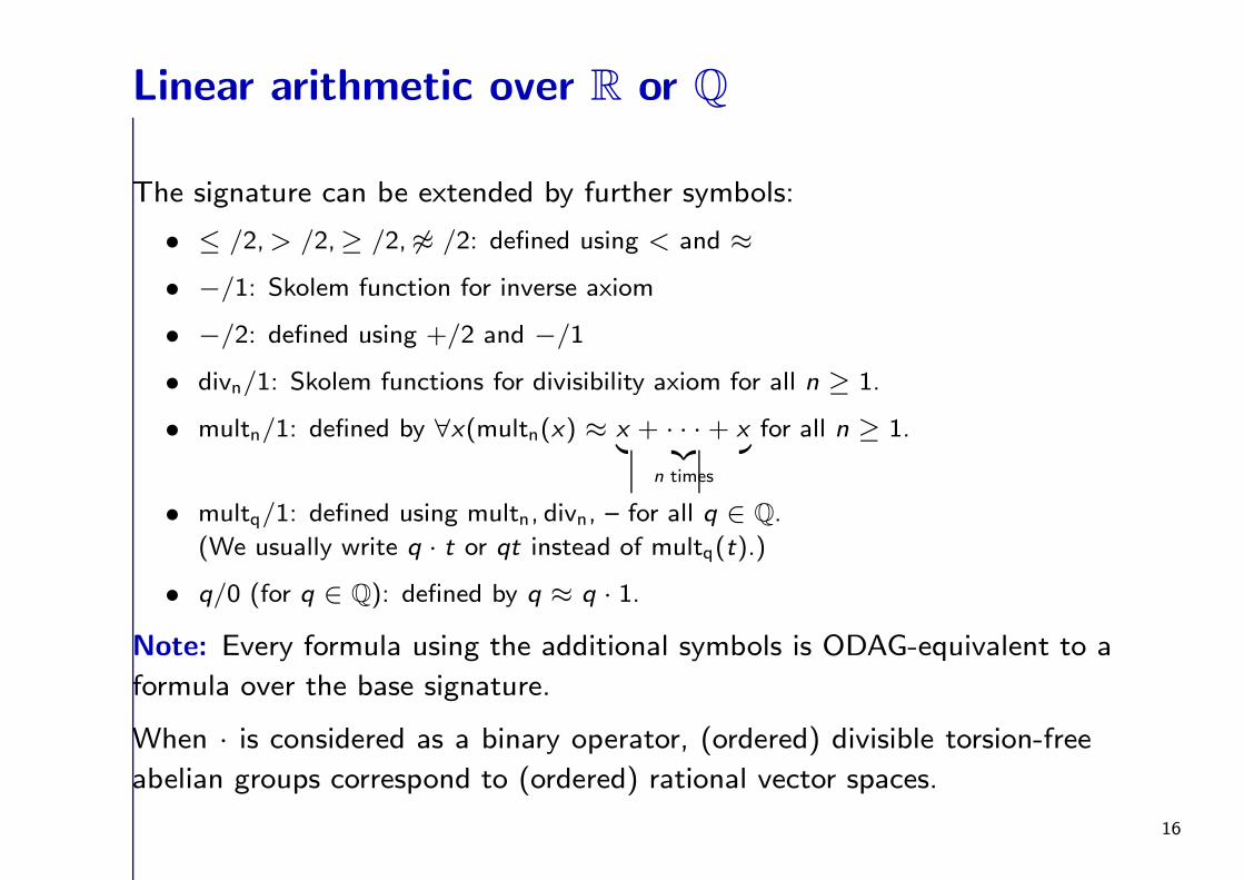
The signature can be extended by further symbols:
• ≤ /2,> /2,≥ /2, 6≈ /2: defined using < and ≈
• −/1: Skolem function for inverse axiom
• −/2: defined using +/2 and −/1
• divn/1: Skolem functions for divisibility axiom for all n ≥ 1.
• multn/1: defined by ∀x(multn(x) ≈ x + · · · + x︸ ︷︷ ︸
n times
for all n ≥ 1.
• multq/1: defined using multn, divn, – for all q ∈ Q.
(We usually write q · t or qt instead of multq(t).)
• q/0 (for q ∈ Q): defined by q ≈ q · 1.
Note: Every formula using the additional symbols is ODAG-equivalent to a
formula over the base signature.
When · is considered as a binary operator, (ordered) divisible torsion-free
abelian groups correspond to (ordered) rational vector spaces.
16
Linear arithmetic over R or Q
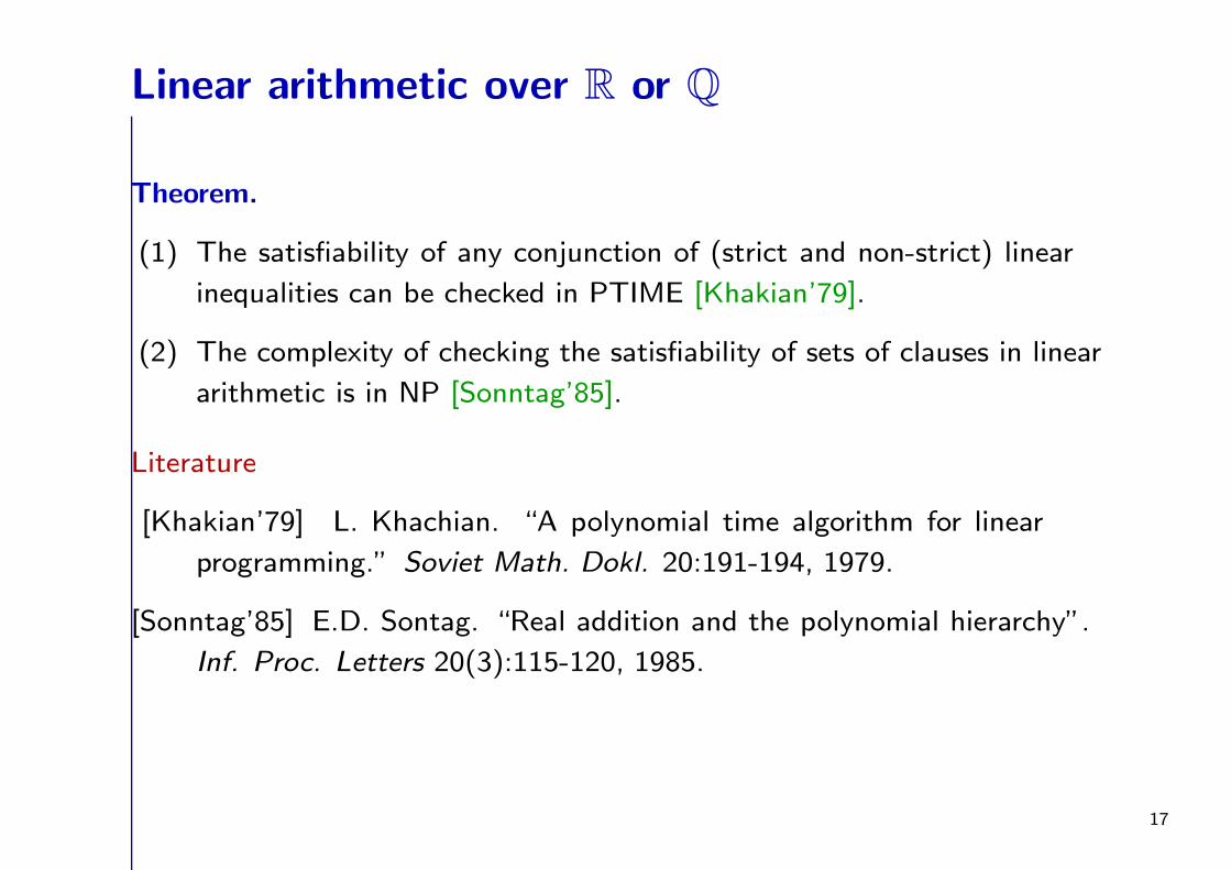
Theorem.
(1) The satisfiability of any conjunction of (strict and non-strict) linear
inequalities can be checked in PTIME [Khakian’79].
(2) The complexity of checking the satisfiability of sets of clauses in linear
arithmetic is in NP [Sonntag’85].
Literature
[Khakian’79] L. Khachian. “A polynomial time algorithm for linear
programming.” Soviet Math. Dokl. 20:191-194, 1979.
[Sonntag’85] E.D. Sontag. “Real addition and the polynomial hierarchy”.
Inf. Proc. Letters 20(3):115-120, 1985.
17
Linear arithmetic over R or Q
Methods The algorithms currently used are not PTIME.
• The simplex method
• The Fourier-Motzkin method – use variable elimination
18
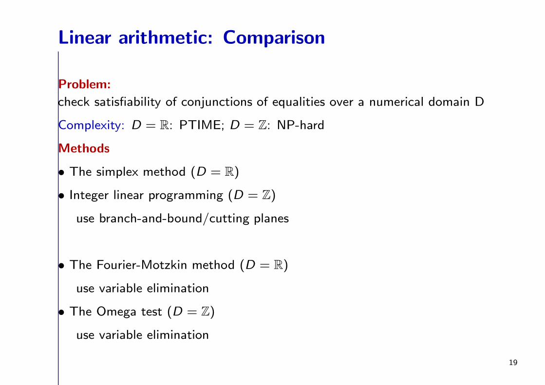
Linear arithmetic: Comparison
Problem:
check satisfiability of conjunctions of equalities over a numerical domain D
Complexity: D = R: PTIME; D = Z: NP-hard
Methods
• The simplex method (D = R)
• Integer linear programming (D = Z)
use branch-and-bound/cutting planes
• The Fourier-Motzkin method (D = R)
use variable elimination
• The Omega test (D = Z)
use variable elimination
19
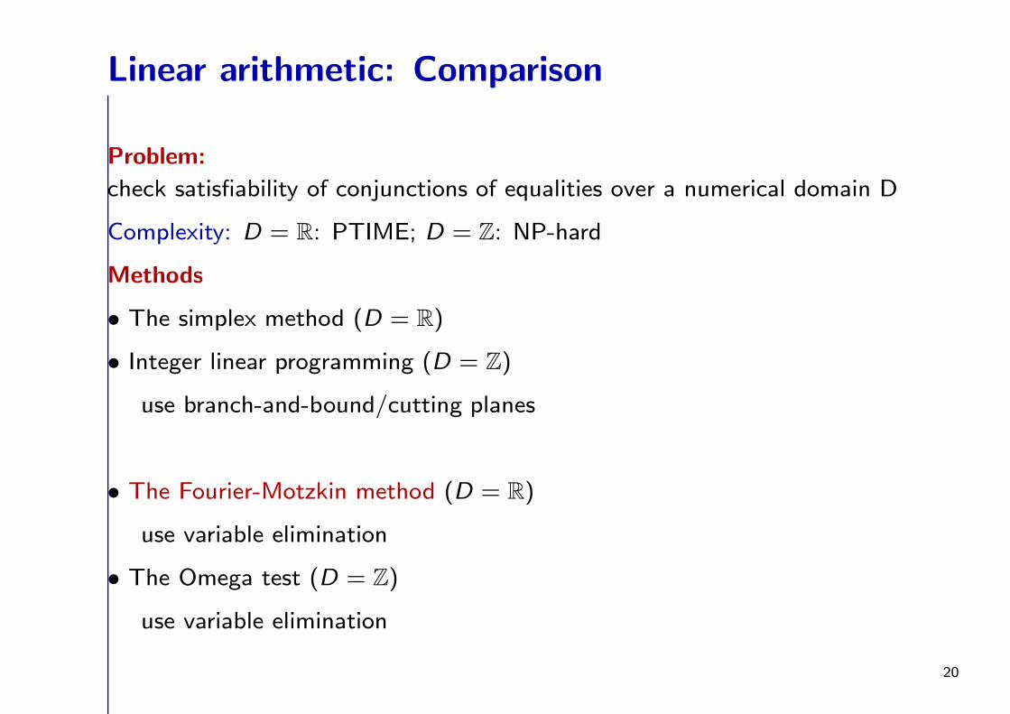
Linear arithmetic: Comparison
Problem:
check satisfiability of conjunctions of equalities over a numerical domain D
Complexity: D = R: PTIME; D = Z: NP-hard
Methods
• The simplex method (D = R)
• Integer linear programming (D = Z)
use branch-and-bound/cutting planes
• The Fourier-Motzkin method (D = R)
use variable elimination
• The Omega test (D = Z)
use variable elimination
20
Fourier-Motzkin Quantifier Elimination
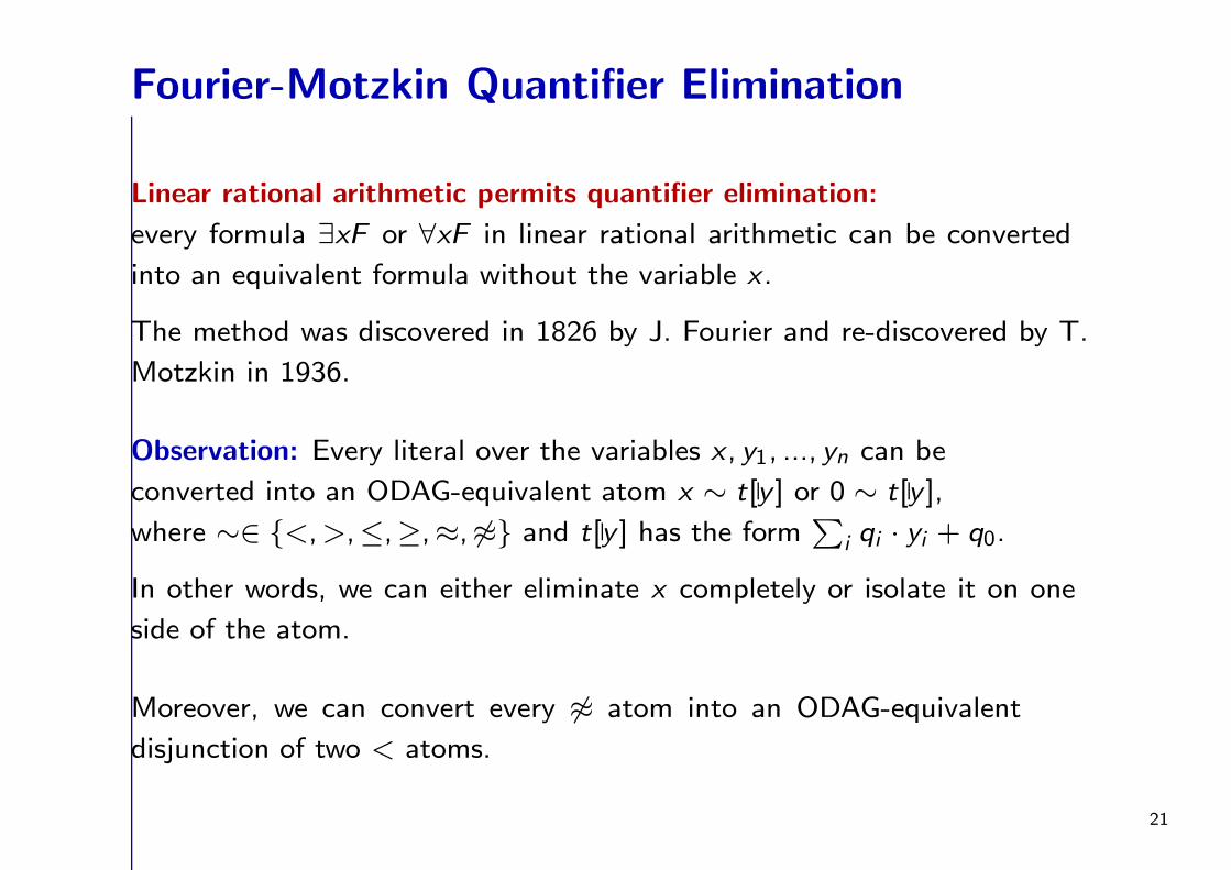
Linear rational arithmetic permits quantifier elimination:
every formula ∃xF or ∀xF in linear rational arithmetic can be converted
into an equivalent formula without the variable x .
The method was discovered in 1826 by J. Fourier and re-discovered by T.
Motzkin in 1936.
Observation: Every literal over the variables x , y1, ..., yn can be
converted into an ODAG-equivalent atom x ∼ t[y ] or 0 ∼ t[y ],
where ∼∈ <,>,≤,≥,≈, 6≈ and t[y ] has the form∑
i qi · yi + q0.
In other words, we can either eliminate x completely or isolate it on one
side of the atom.
Moreover, we can convert every 6≈ atom into an ODAG-equivalent
disjunction of two < atoms.
21
Fourier-Motzkin Quantifier Elimination
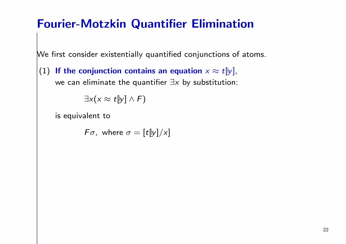
We first consider existentially quantified conjunctions of atoms.
(1) If the conjunction contains an equation x ≈ t[y ],
we can eliminate the quantifier ∃x by substitution:
∃x(x ≈ t[y ] ∧ F )
is equivalent to
Fσ, where σ = [t[y ]/x]
22
Fourier-Motzkin Quantifier Elimination
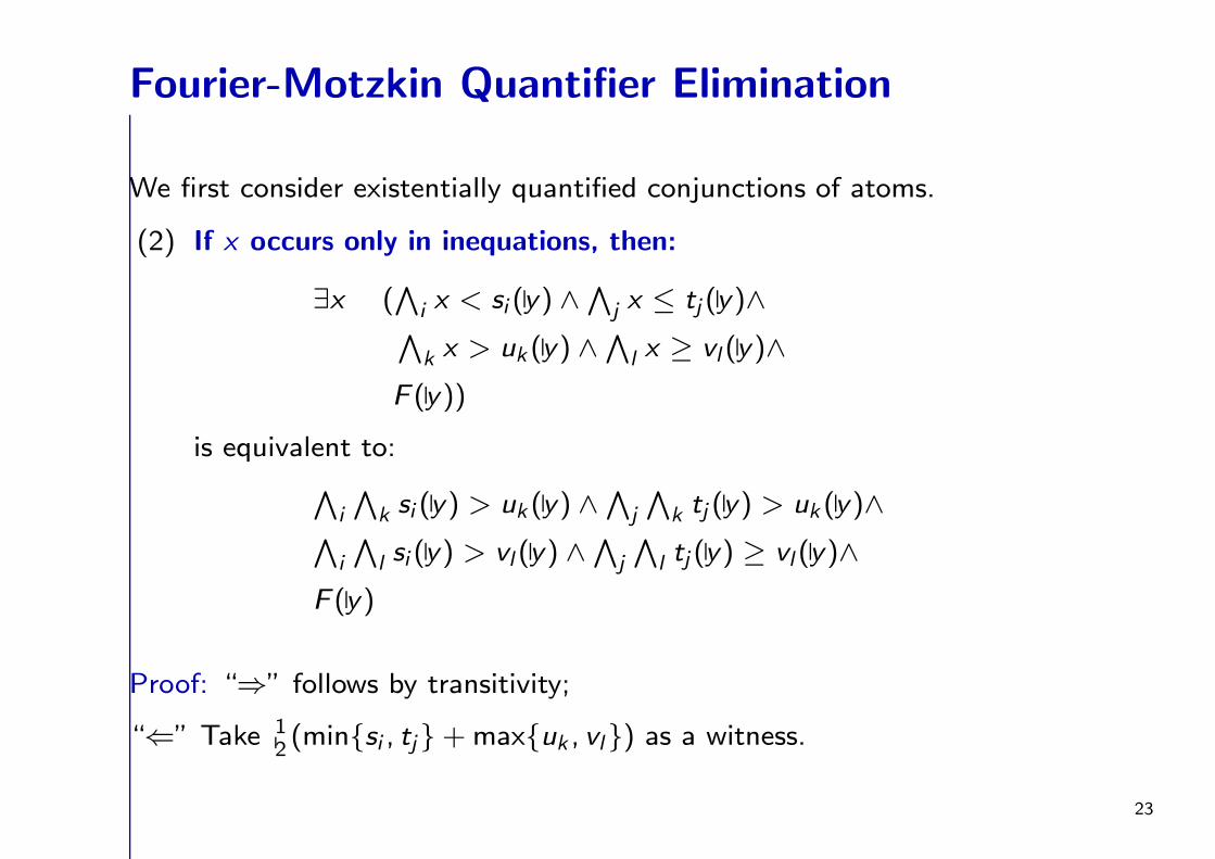
We first consider existentially quantified conjunctions of atoms.
(2) If x occurs only in inequations, then:
∃x (∧
i x < si (y) ∧∧
j x ≤ tj (y)∧∧
k x > uk (y) ∧∧
l x ≥ vl (y)∧
F (y))
is equivalent to:∧
i
∧
k si (y) > uk (y) ∧∧
j
∧
k tj (y) > uk (y)∧∧
i
∧
l si (y) > vl (y) ∧∧
j
∧
l tj (y) ≥ vl (y)∧
F (y)
Proof: “⇒” follows by transitivity;
“⇐” Take 12(minsi , tj+maxuk , vl) as a witness.
23
Fourier-Motzkin Quantifier Elimination
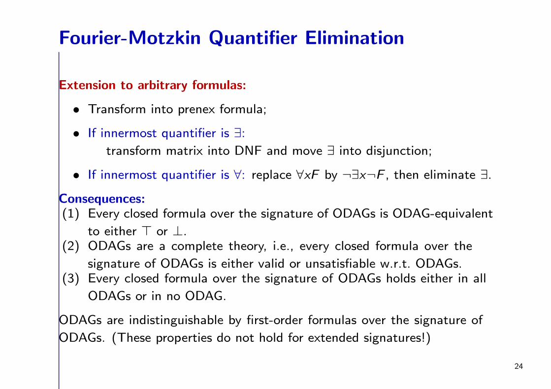
Extension to arbitrary formulas:
• Transform into prenex formula;
• If innermost quantifier is ∃:
transform matrix into DNF and move ∃ into disjunction;
• If innermost quantifier is ∀: replace ∀xF by ¬∃x¬F , then eliminate ∃.
Consequences:(1) Every closed formula over the signature of ODAGs is ODAG-equivalent
to either ⊤ or ⊥.(2) ODAGs are a complete theory, i.e., every closed formula over the
signature of ODAGs is either valid or unsatisfiable w.r.t. ODAGs.(3) Every closed formula over the signature of ODAGs holds either in all
ODAGs or in no ODAG.
ODAGs are indistinguishable by first-order formulas over the signature of
ODAGs. (These properties do not hold for extended signatures!)
24
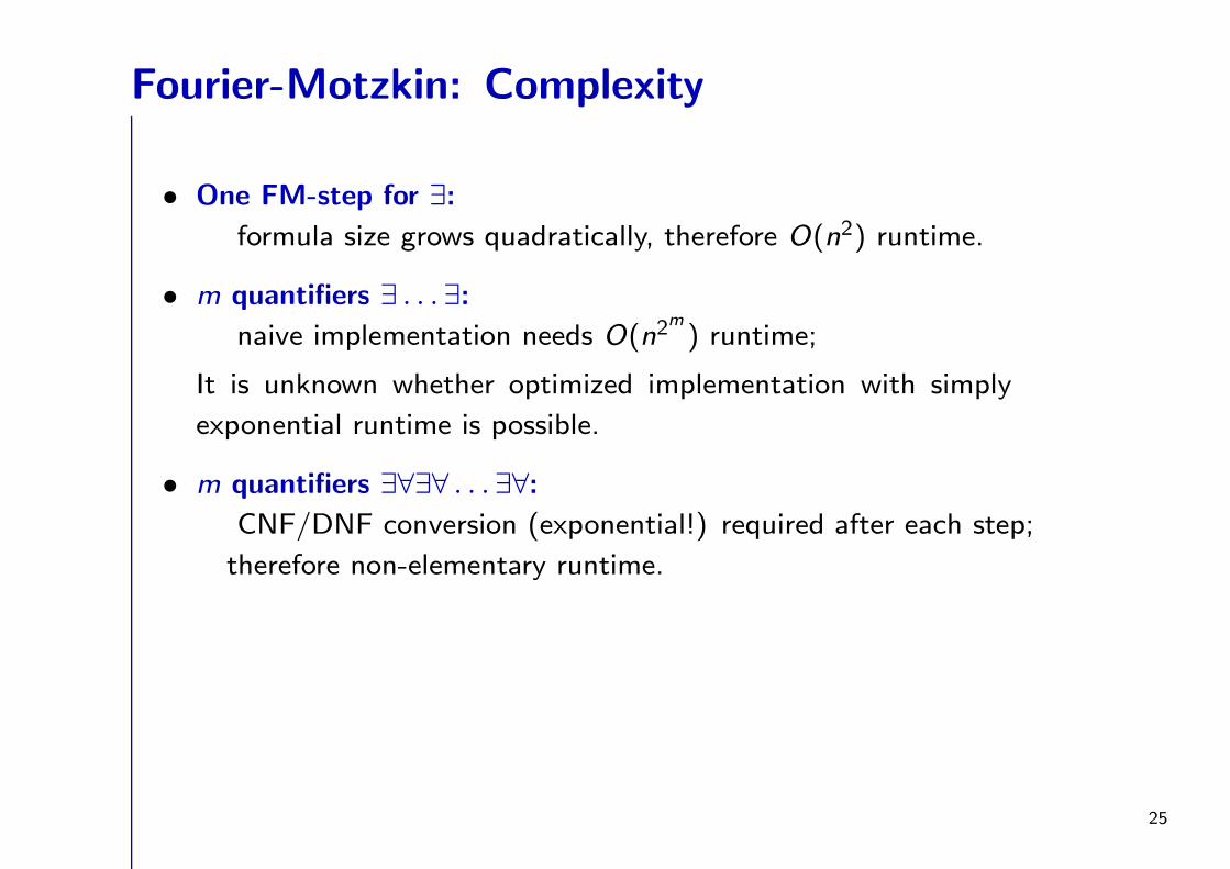
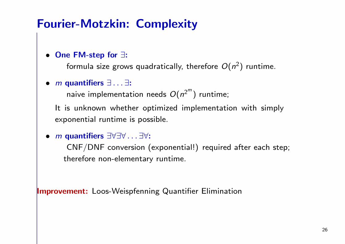
Fourier-Motzkin: Complexity
• One FM-step for ∃:
formula size grows quadratically, therefore O(n2) runtime.
• m quantifiers ∃ . . . ∃:
naive implementation needs O(n2m) runtime;
It is unknown whether optimized implementation with simply
exponential runtime is possible.
• m quantifiers ∃∀∃∀ . . . ∃∀:
CNF/DNF conversion (exponential!) required after each step;
therefore non-elementary runtime.
25
Fourier-Motzkin: Complexity
• One FM-step for ∃:
formula size grows quadratically, therefore O(n2) runtime.
• m quantifiers ∃ . . . ∃:
naive implementation needs O(n2m) runtime;
It is unknown whether optimized implementation with simply
exponential runtime is possible.
• m quantifiers ∃∀∃∀ . . . ∃∀:
CNF/DNF conversion (exponential!) required after each step;
therefore non-elementary runtime.
Improvement: Loos-Weispfenning Quantifier Elimination
26
Loos-Weispfenning Quantifier Elimination
A more efficient way to eliminate quantifiers in linear rational arithmetic
was developed by R. Loos and V. Weispfenning (1993).
The method is also known as “test point method” or “virtual substitution
method”.
For simplicity, we consider only one particular ODAG, namely Q (as we
have seen above, the results are the same for all ODAGs).
27
Loos-Weispfenning Quantifier Elimination
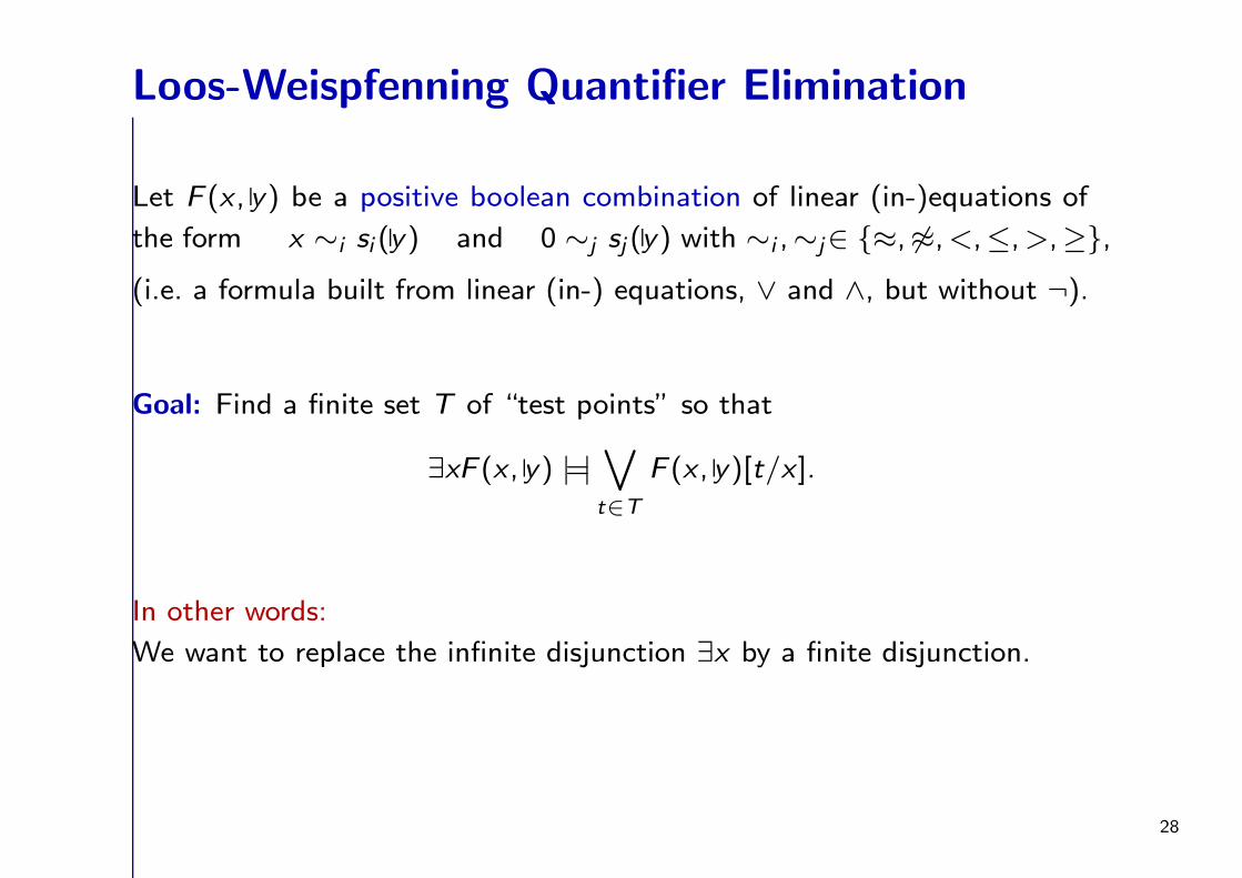
Let F (x , y) be a positive boolean combination of linear (in-)equations of
the form x ∼i si (y) and 0 ∼j sj (y) with ∼i ,∼j∈ ≈, 6≈,<,≤,>,≥,
(i.e. a formula built from linear (in-) equations, ∨ and ∧, but without ¬).
Goal: Find a finite set T of “test points” so that
∃xF (x , y) |=|∨
t∈T
F (x , y)[t/x].
In other words:
We want to replace the infinite disjunction ∃x by a finite disjunction.
28
Loos-Weispfenning Quantifier Elimination
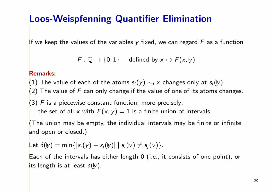
If we keep the values of the variables y fixed, we can regard F as a function
F : Q → 0, 1 defined by x 7→ F (x , y)
Remarks:
(1) The value of each of the atoms si (y) ∼i x changes only at si (y),
(2) The value of F can only change if the value of one of its atoms changes.
(3) F is a piecewise constant function; more precisely:
the set of all x with F (x , y) = 1 is a finite union of intervals.
(The union may be empty, the individual intervals may be finite or infinite
and open or closed.)
Let δ(y) = min|si (y)− sj (y)| | si (y) 6= sj (y).
Each of the intervals has either length 0 (i.e., it consists of one point), or
its length is at least δ(y).
29
Loos-Weispfenning Quantifier Elimination
If the set of all x for which F (x , y) is 1 is non-empty, then
(i) F (x , y) = 1 for all x ≤ r(y) for some r(y) ∈ Q
(ii) or there is some point where the value of F (x , y) switches from 0 to 1
when we traverse the real axis from −∞ to +∞.
We use this observation to construct a set of test points.
30
Loos-Weispfenning Quantifier Elimination
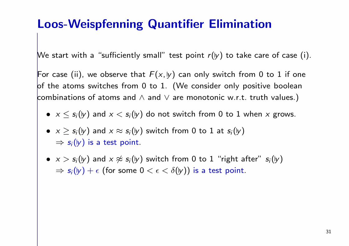
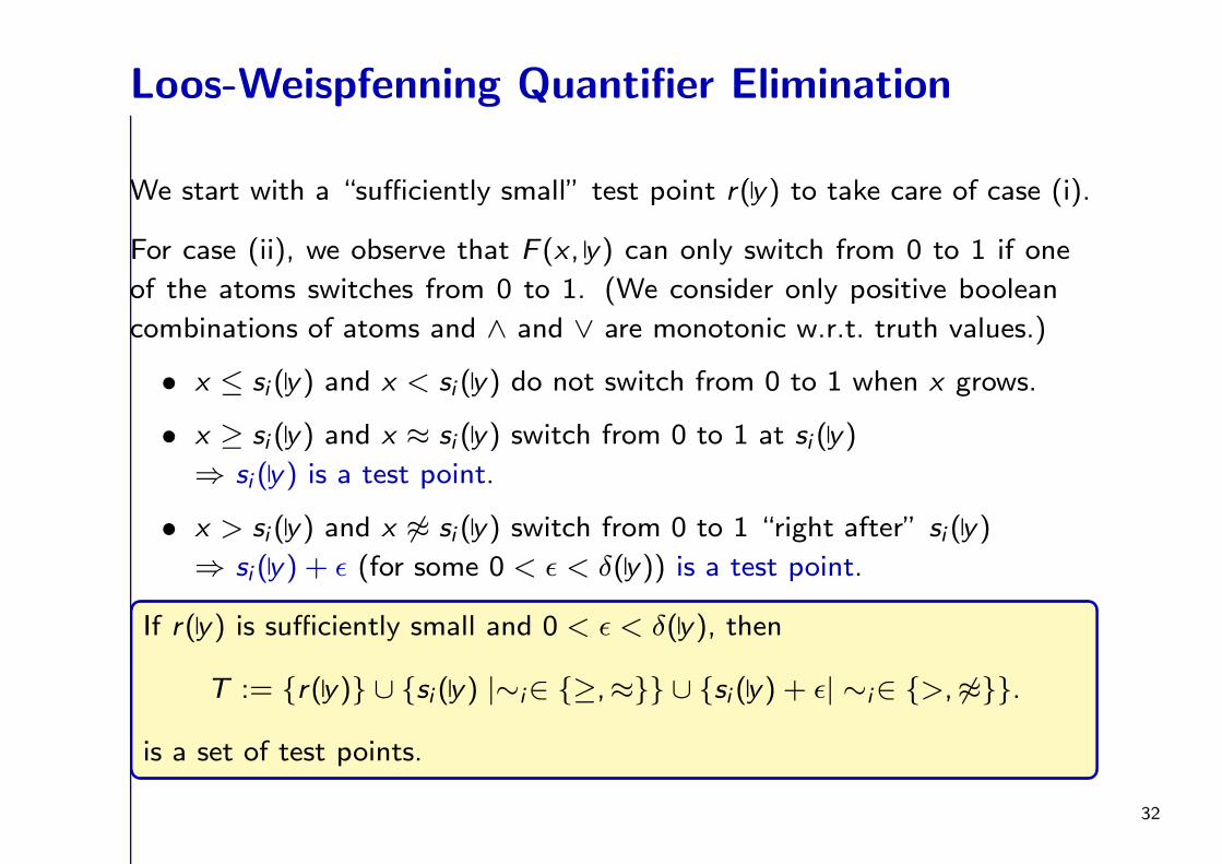
We start with a “sufficiently small” test point r(y) to take care of case (i).
For case (ii), we observe that F (x , y) can only switch from 0 to 1 if one
of the atoms switches from 0 to 1. (We consider only positive boolean
combinations of atoms and ∧ and ∨ are monotonic w.r.t. truth values.)
• x ≤ si (y) and x < si (y) do not switch from 0 to 1 when x grows.
• x ≥ si (y) and x ≈ si (y) switch from 0 to 1 at si (y)
⇒ si (y) is a test point.
• x > si (y) and x 6≈ si (y) switch from 0 to 1 “right after” si (y)
⇒ si (y) + ǫ (for some 0 < ǫ < δ(y)) is a test point.
31
Loos-Weispfenning Quantifier Elimination
We start with a “sufficiently small” test point r(y) to take care of case (i).
For case (ii), we observe that F (x , y) can only switch from 0 to 1 if one
of the atoms switches from 0 to 1. (We consider only positive boolean
combinations of atoms and ∧ and ∨ are monotonic w.r.t. truth values.)
• x ≤ si (y) and x < si (y) do not switch from 0 to 1 when x grows.
• x ≥ si (y) and x ≈ si (y) switch from 0 to 1 at si (y)
⇒ si (y) is a test point.
• x > si (y) and x 6≈ si (y) switch from 0 to 1 “right after” si (y)
⇒ si (y) + ǫ (for some 0 < ǫ < δ(y)) is a test point.
If r(y) is sufficiently small and 0 < ǫ < δ(y), then
T := r(y) ∪ si (y) |∼i∈ ≥,≈ ∪ si (y) + ǫ| ∼i∈ >, 6≈.
is a set of test points.
32
Loos-Weispfenning Quantifier Elimination
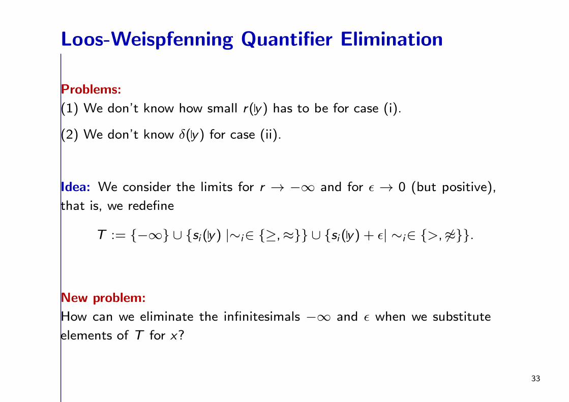
Problems:
(1) We don’t know how small r(y) has to be for case (i).
(2) We don’t know δ(y) for case (ii).
Idea: We consider the limits for r → −∞ and for ǫ → 0 (but positive),
that is, we redefine
T := −∞ ∪ si (y) |∼i∈ ≥,≈ ∪ si (y) + ǫ| ∼i∈ >, 6≈.
New problem:
How can we eliminate the infinitesimals −∞ and ǫ when we substitute
elements of T for x?
33
Loos-Weispfenning Quantifier Elimination
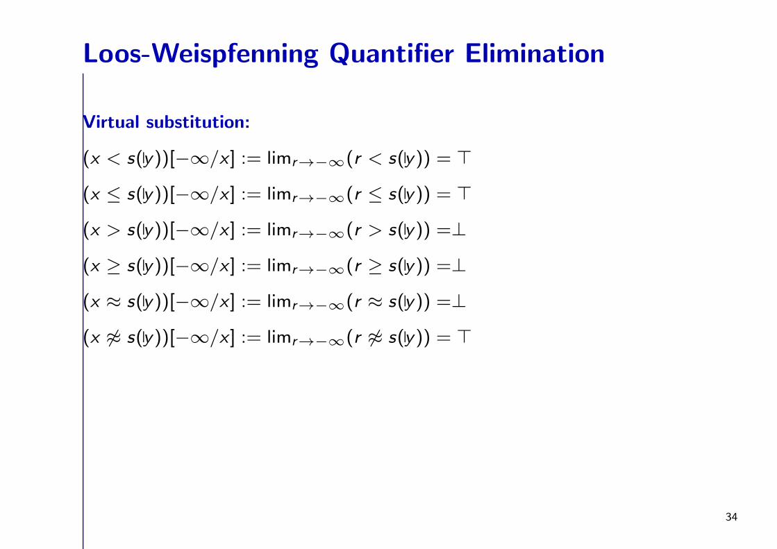
Virtual substitution:
(x < s(y))[−∞/x] := limr→−∞(r < s(y)) = ⊤
(x ≤ s(y))[−∞/x] := limr→−∞(r ≤ s(y)) = ⊤
(x > s(y))[−∞/x] := limr→−∞(r > s(y)) =⊥
(x ≥ s(y))[−∞/x] := limr→−∞(r ≥ s(y)) =⊥
(x ≈ s(y))[−∞/x] := limr→−∞(r ≈ s(y)) =⊥
(x 6≈ s(y))[−∞/x] := limr→−∞(r 6≈ s(y)) = ⊤
34
Loos-Weispfenning Quantifier Elimination
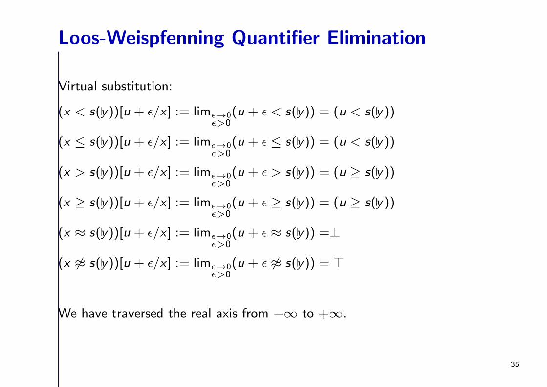
Virtual substitution:
(x < s(y))[u + ǫ/x] := limǫ→0ǫ>0
(u + ǫ < s(y)) = (u < s(y))
(x ≤ s(y))[u + ǫ/x] := limǫ→0ǫ>0
(u + ǫ ≤ s(y)) = (u < s(y))
(x > s(y))[u + ǫ/x] := limǫ→0ǫ>0
(u + ǫ > s(y)) = (u ≥ s(y))
(x ≥ s(y))[u + ǫ/x] := limǫ→0ǫ>0
(u + ǫ ≥ s(y)) = (u ≥ s(y))
(x ≈ s(y))[u + ǫ/x] := limǫ→0ǫ>0
(u + ǫ ≈ s(y)) =⊥
(x 6≈ s(y))[u + ǫ/x] := limǫ→0ǫ>0
(u + ǫ 6≈ s(y)) = ⊤
We have traversed the real axis from −∞ to +∞.
35
Loos-Weispfenning Quantifier Elimination
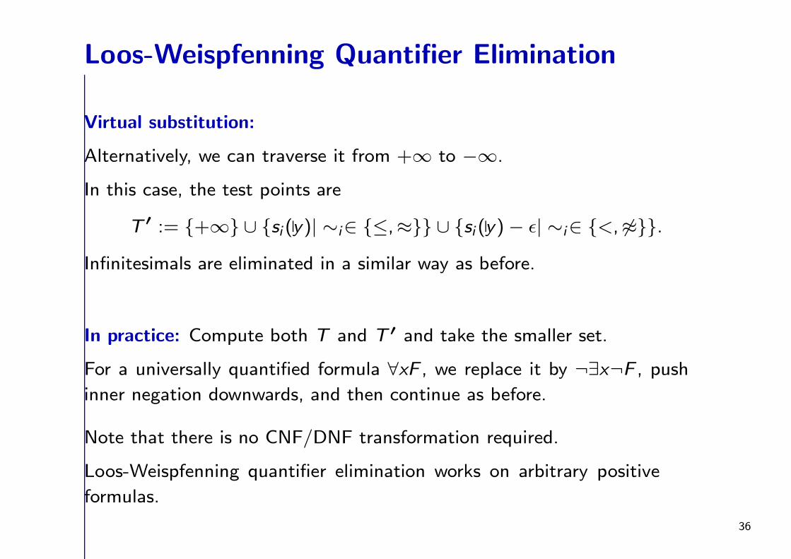
Virtual substitution:
Alternatively, we can traverse it from +∞ to −∞.
In this case, the test points are
T ′ := +∞∪ si (y)| ∼i∈ ≤,≈ ∪ si (y)− ǫ| ∼i∈ <, 6≈.
Infinitesimals are eliminated in a similar way as before.
In practice: Compute both T and T ′ and take the smaller set.
For a universally quantified formula ∀xF , we replace it by ¬∃x¬F , push
inner negation downwards, and then continue as before.
Note that there is no CNF/DNF transformation required.
Loos-Weispfenning quantifier elimination works on arbitrary positive
formulas.
36
Loos-Weispfenning: Complexity
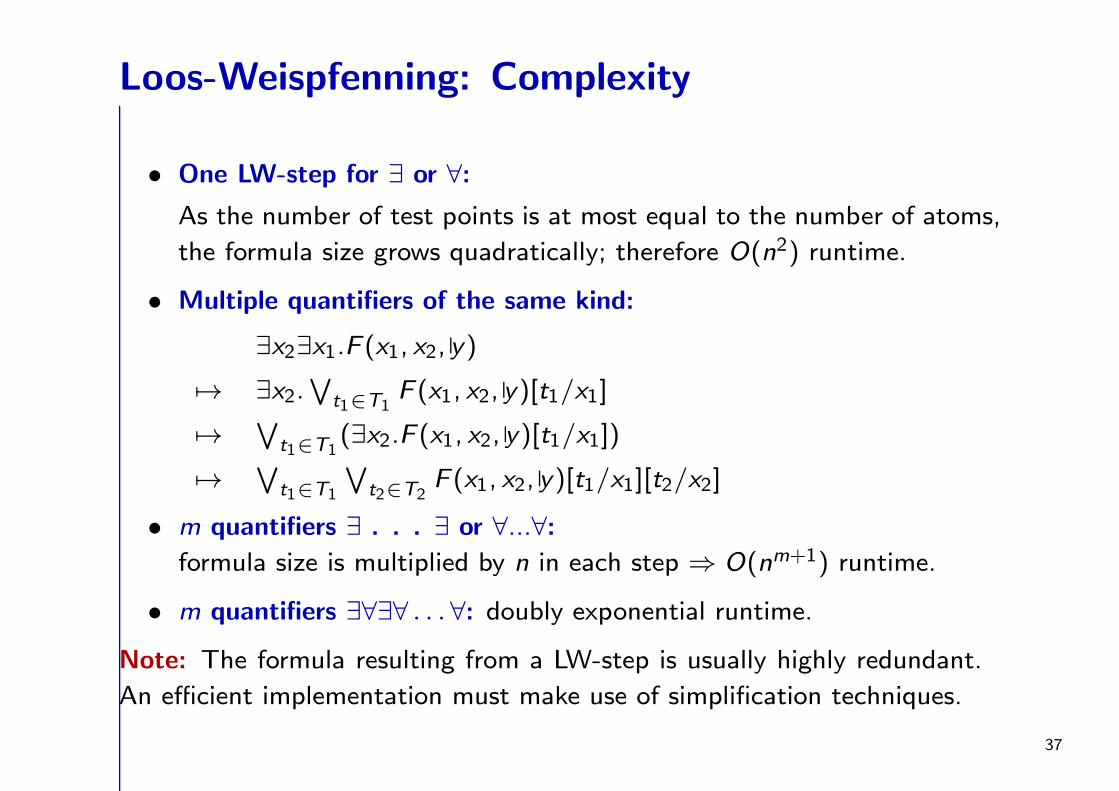
• One LW-step for ∃ or ∀:
As the number of test points is at most equal to the number of atoms,
the formula size grows quadratically; therefore O(n2) runtime.
• Multiple quantifiers of the same kind:
∃x2∃x1.F (x1, x2, y)
7→ ∃x2.∨
t1∈T1F (x1, x2, y)[t1/x1]
7→∨
t1∈T1(∃x2.F (x1, x2, y)[t1/x1])
7→∨
t1∈T1
∨
t2∈T2F (x1, x2, y)[t1/x1][t2/x2]
• m quantifiers ∃ . . . ∃ or ∀...∀:
formula size is multiplied by n in each step ⇒ O(nm+1) runtime.
• m quantifiers ∃∀∃∀ . . . ∀: doubly exponential runtime.
Note: The formula resulting from a LW-step is usually highly redundant.
An efficient implementation must make use of simplification techniques.
37
Until now
Decidable fragments of first-order logic
Decision procedures for single theories
• UIF
• Numeric domains
Here:
Difference logic
Linear arithmetic over R, Q
Next: Reasoning in combinations of theories
Combinations of decision procedures
38
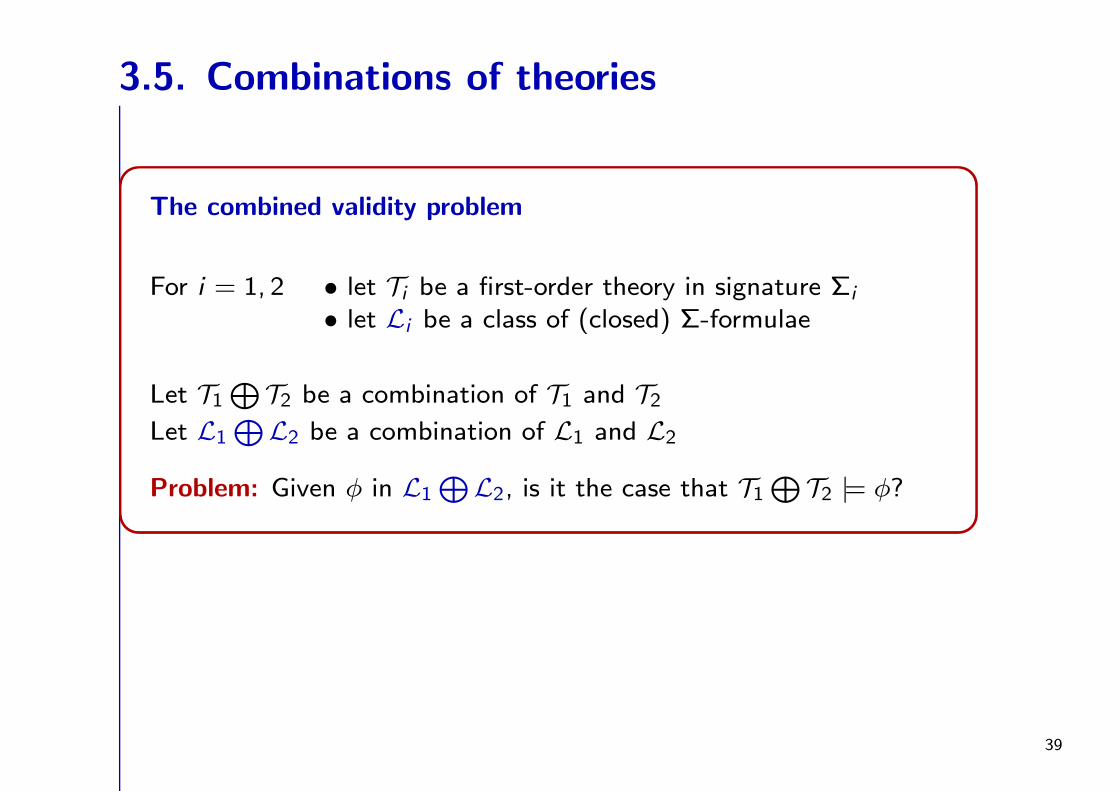
3.5. Combinations of theories
The combined validity problem
For i = 1, 2 • let Ti be a first-order theory in signature Σi
• let Li be a class of (closed) Σ-formulae
Let T1⊕
T2 be a combination of T1 and T2Let L1
⊕L2 be a combination of L1 and L2
Problem: Given φ in L1⊕
L2, is it the case that T1⊕
T2 |= φ?
39
Problems
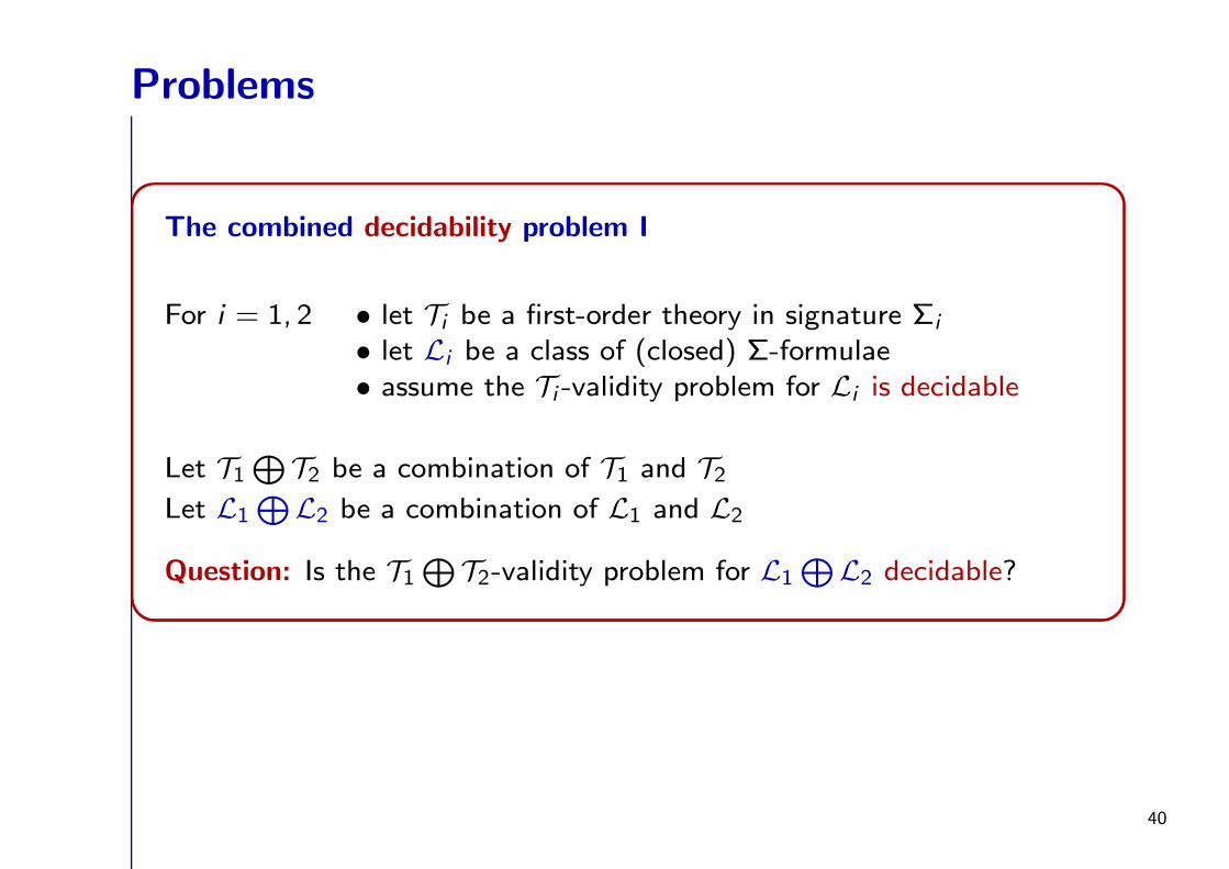
The combined decidability problem I
For i = 1, 2 • let Ti be a first-order theory in signature Σi
• let Li be a class of (closed) Σ-formulae• assume the Ti -validity problem for Li is decidable
Let T1⊕
T2 be a combination of T1 and T2Let L1
⊕L2 be a combination of L1 and L2
Question: Is the T1⊕
T2-validity problem for L1⊕
L2 decidable?
40
Problems
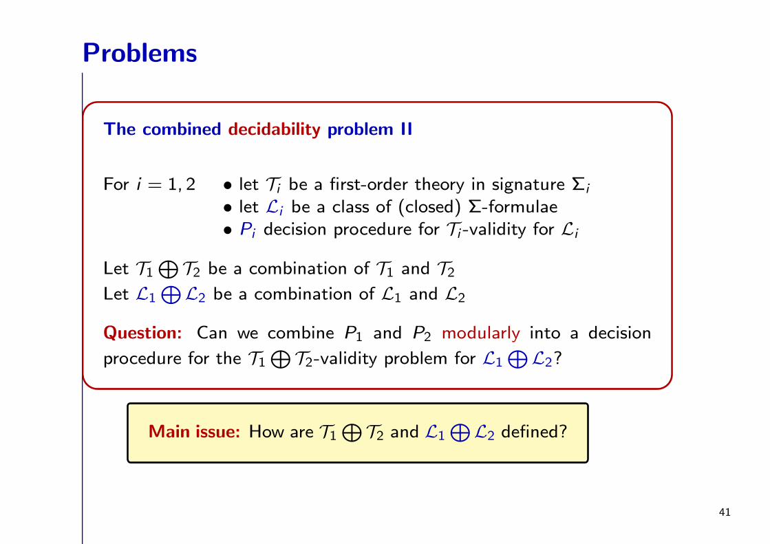
The combined decidability problem II
For i = 1, 2 • let Ti be a first-order theory in signature Σi
• let Li be a class of (closed) Σ-formulae• Pi decision procedure for Ti -validity for Li
Let T1⊕
T2 be a combination of T1 and T2Let L1
⊕L2 be a combination of L1 and L2
Question: Can we combine P1 and P2 modularly into a decision
procedure for the T1⊕
T2-validity problem for L1⊕
L2?
Main issue: How are T1⊕
T2 and L1⊕
L2 defined?
41
Combinations of theories and models
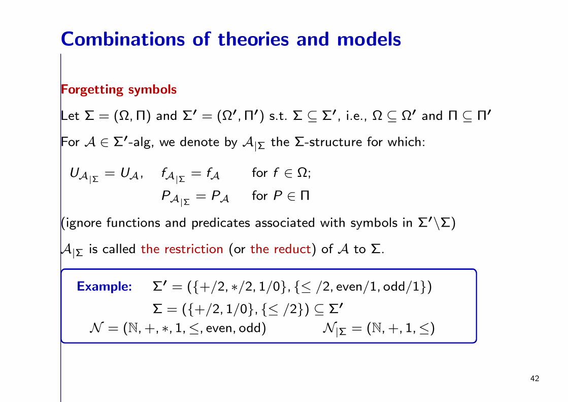
Forgetting symbols
Let Σ = (Ω,Π) and Σ′ = (Ω′, Π′) s.t. Σ ⊆ Σ′, i.e., Ω ⊆ Ω′ and Π ⊆ Π′
For A ∈ Σ′-alg, we denote by A|Σ the Σ-structure for which:
UA|Σ= UA, fA|Σ
= fA for f ∈ Ω;
PA|Σ= PA for P ∈ Π
(ignore functions and predicates associated with symbols in Σ′\Σ)
A|Σ is called the restriction (or the reduct) of A to Σ.
Example: Σ′ = (+/2, ∗/2, 1/0, ≤ /2, even/1, odd/1)
Σ = (+/2, 1/0, ≤ /2) ⊆ Σ′
N = (N, +, ∗, 1,≤, even, odd) N|Σ = (N, +, 1,≤)
42
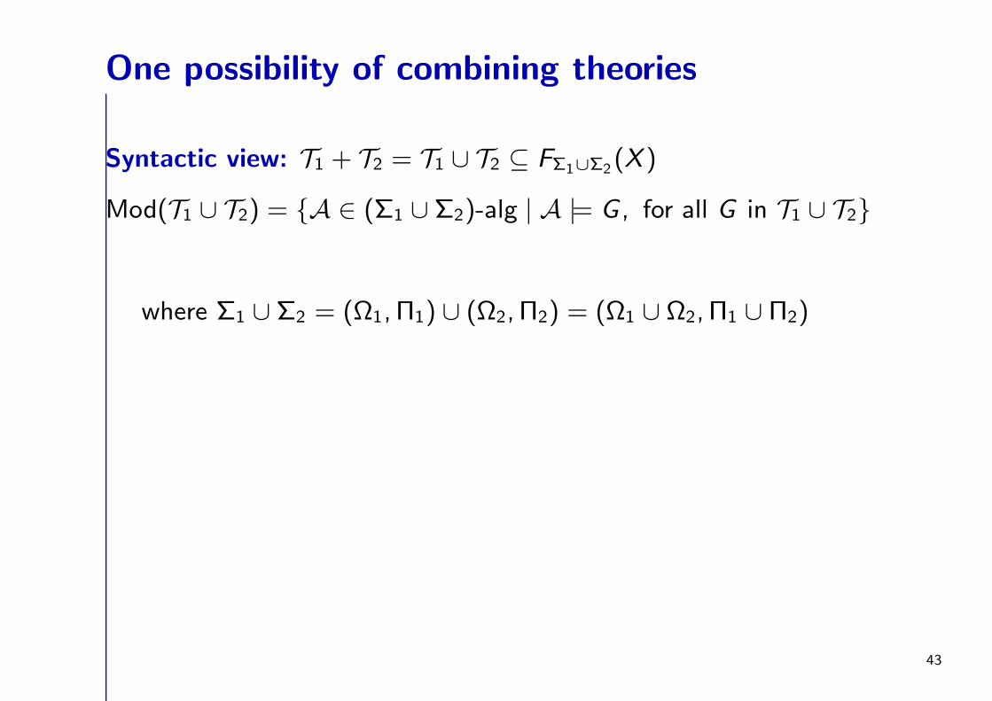
One possibility of combining theories
Syntactic view: T1 + T2 = T1 ∪ T2 ⊆ FΣ1∪Σ2(X )
Mod(T1 ∪ T2) = A ∈ (Σ1 ∪ Σ2)-alg | A |= G , for all G in T1 ∪ T2
where Σ1 ∪ Σ2 = (Ω1, Π1) ∪ (Ω2, Π2) = (Ω1 ∪ Ω2, Π1 ∪ Π2)
43
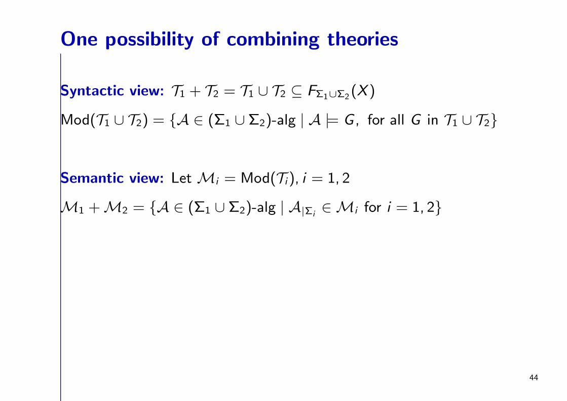
One possibility of combining theories
Syntactic view: T1 + T2 = T1 ∪ T2 ⊆ FΣ1∪Σ2(X )
Mod(T1 ∪ T2) = A ∈ (Σ1 ∪ Σ2)-alg | A |= G , for all G in T1 ∪ T2
Semantic view: Let Mi = Mod(Ti), i = 1, 2
M1 +M2 = A ∈ (Σ1 ∪ Σ2)-alg | A|Σi∈ Mi for i = 1, 2
44
One possibility of combining theories
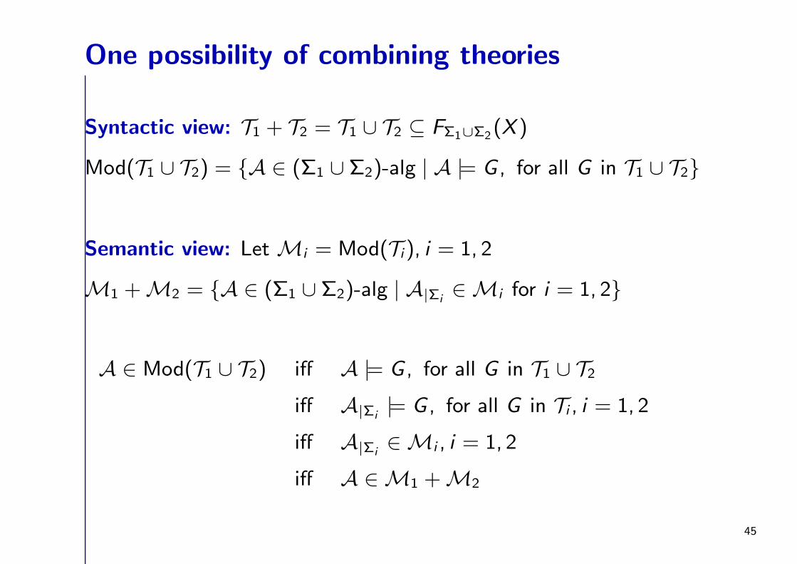
Syntactic view: T1 + T2 = T1 ∪ T2 ⊆ FΣ1∪Σ2(X )
Mod(T1 ∪ T2) = A ∈ (Σ1 ∪ Σ2)-alg | A |= G , for all G in T1 ∪ T2
Semantic view: Let Mi = Mod(Ti), i = 1, 2
M1 +M2 = A ∈ (Σ1 ∪ Σ2)-alg | A|Σi∈ Mi for i = 1, 2
A ∈ Mod(T1 ∪ T2) iff A |= G , for all G in T1 ∪ T2
iff A|Σi|= G , for all G in Ti , i = 1, 2
iff A|Σi∈ Mi , i = 1, 2
iff A ∈ M1 +M2
45
One possibility of combining theories
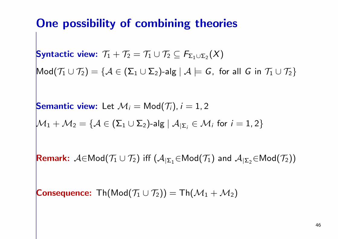
Syntactic view: T1 + T2 = T1 ∪ T2 ⊆ FΣ1∪Σ2(X )
Mod(T1 ∪ T2) = A ∈ (Σ1 ∪ Σ2)-alg | A |= G , for all G in T1 ∪ T2
Semantic view: Let Mi = Mod(Ti), i = 1, 2
M1 +M2 = A ∈ (Σ1 ∪ Σ2)-alg | A|Σi∈ Mi for i = 1, 2
Remark: A∈Mod(T1 ∪ T2) iff (A|Σ1∈Mod(T1) and A|Σ2
∈Mod(T2))
Consequence: Th(Mod(T1 ∪ T2)) = Th(M1 +M2)
46
Example
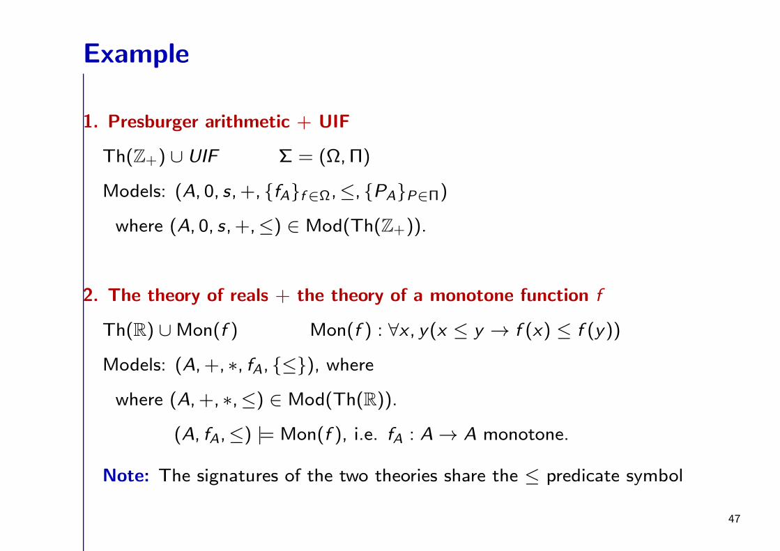
1. Presburger arithmetic + UIF
Th(Z+) ∪ UIF Σ = (Ω,Π)
Models: (A, 0, s, +, fAf∈Ω,≤, PAP∈Π)
where (A, 0, s, +,≤) ∈ Mod(Th(Z+)).
2. The theory of reals + the theory of a monotone function f
Th(R) ∪Mon(f ) Mon(f ) : ∀x , y(x ≤ y → f (x) ≤ f (y))
Models: (A, +, ∗, fA, ≤), where
where (A, +, ∗,≤) ∈ Mod(Th(R)).
(A, fA,≤) |= Mon(f ), i.e. fA : A → A monotone.
Note: The signatures of the two theories share the ≤ predicate symbol
47
Combinations of theories
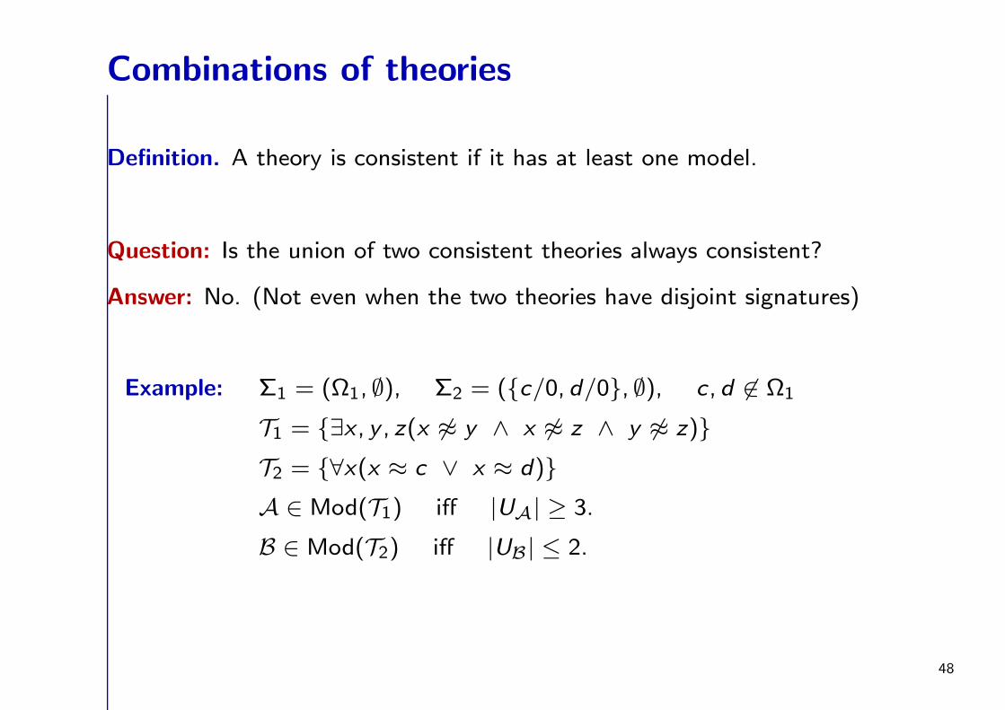
Definition. A theory is consistent if it has at least one model.
Question: Is the union of two consistent theories always consistent?
Answer: No. (Not even when the two theories have disjoint signatures)
Example: Σ1 = (Ω1, ∅), Σ2 = (c/0, d/0, ∅), c, d 6∈ Ω1
T1 = ∃x , y , z(x 6≈ y ∧ x 6≈ z ∧ y 6≈ z)
T2 = ∀x(x ≈ c ∨ x ≈ d)
A ∈ Mod(T1) iff |UA| ≥ 3.
B ∈ Mod(T2) iff |UB| ≤ 2.
48
Combinations of theories
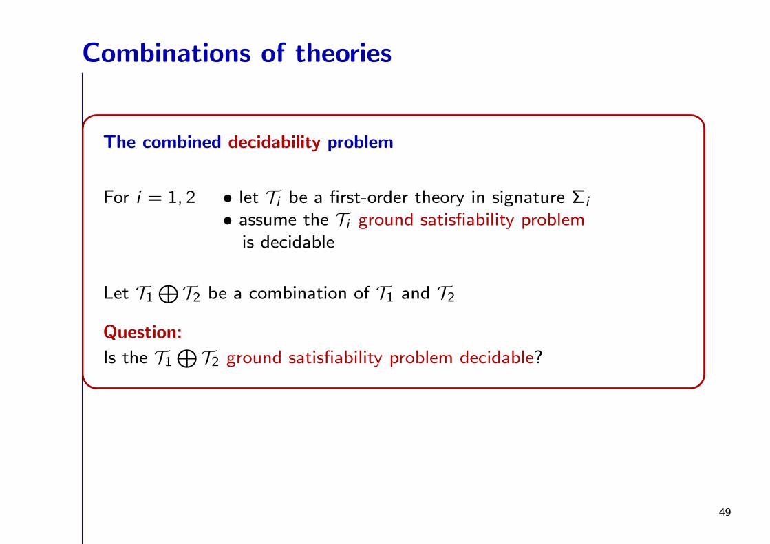
The combined decidability problem
For i = 1, 2 • let Ti be a first-order theory in signature Σi
• assume the Ti ground satisfiability problemis decidable
Let T1⊕
T2 be a combination of T1 and T2
Question:
Is the T1⊕
T2 ground satisfiability problem decidable?
49
Goal: Modularity
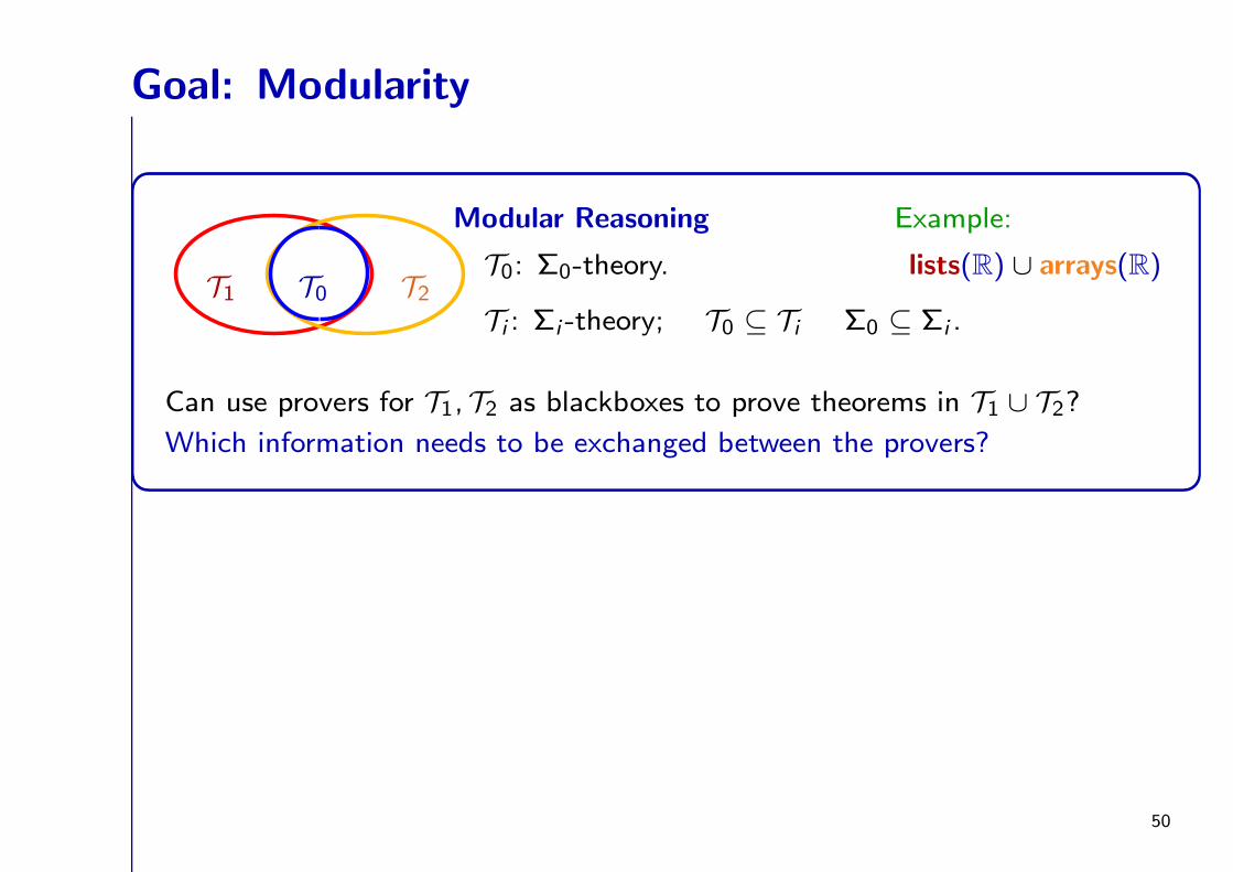
Modular Reasoning Example:
T1 T0 T2T0: Σ0-theory. lists(R) ∪ arrays(R)
Ti : Σi -theory; T0 ⊆ Ti Σ0 ⊆ Σi .
Can use provers for T1, T2 as blackboxes to prove theorems in T1 ∪ T2?
Which information needs to be exchanged between the provers?
50
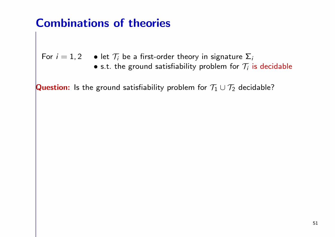
Combinations of theories
For i = 1, 2 • let Ti be a first-order theory in signature Σi
• s.t. the ground satisfiability problem for Ti is decidable
Question: Is the ground satisfiability problem for T1 ∪ T2 decidable?
51
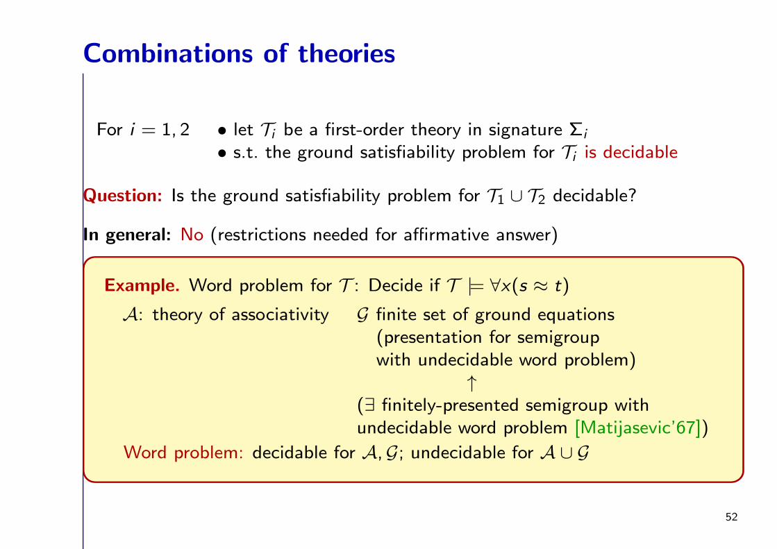
Combinations of theories
For i = 1, 2 • let Ti be a first-order theory in signature Σi
• s.t. the ground satisfiability problem for Ti is decidable
Question: Is the ground satisfiability problem for T1 ∪ T2 decidable?
In general: No (restrictions needed for affirmative answer)
Example. Word problem for T : Decide if T |= ∀x(s ≈ t)
A: theory of associativity G finite set of ground equations(presentation for semigroupwith undecidable word problem)
↑(∃ finitely-presented semigroup withundecidable word problem [Matijasevic’67])
Word problem: decidable for A,G; undecidable for A ∪ G
52
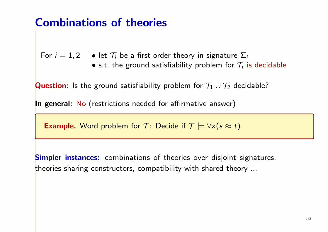
Combinations of theories
For i = 1, 2 • let Ti be a first-order theory in signature Σi
• s.t. the ground satisfiability problem for Ti is decidable
Question: Is the ground satisfiability problem for T1 ∪ T2 decidable?
In general: No (restrictions needed for affirmative answer)
Example. Word problem for T : Decide if T |= ∀x(s ≈ t)
Simpler instances: combinations of theories over disjoint signatures,
theories sharing constructors, compatibility with shared theory ...
53
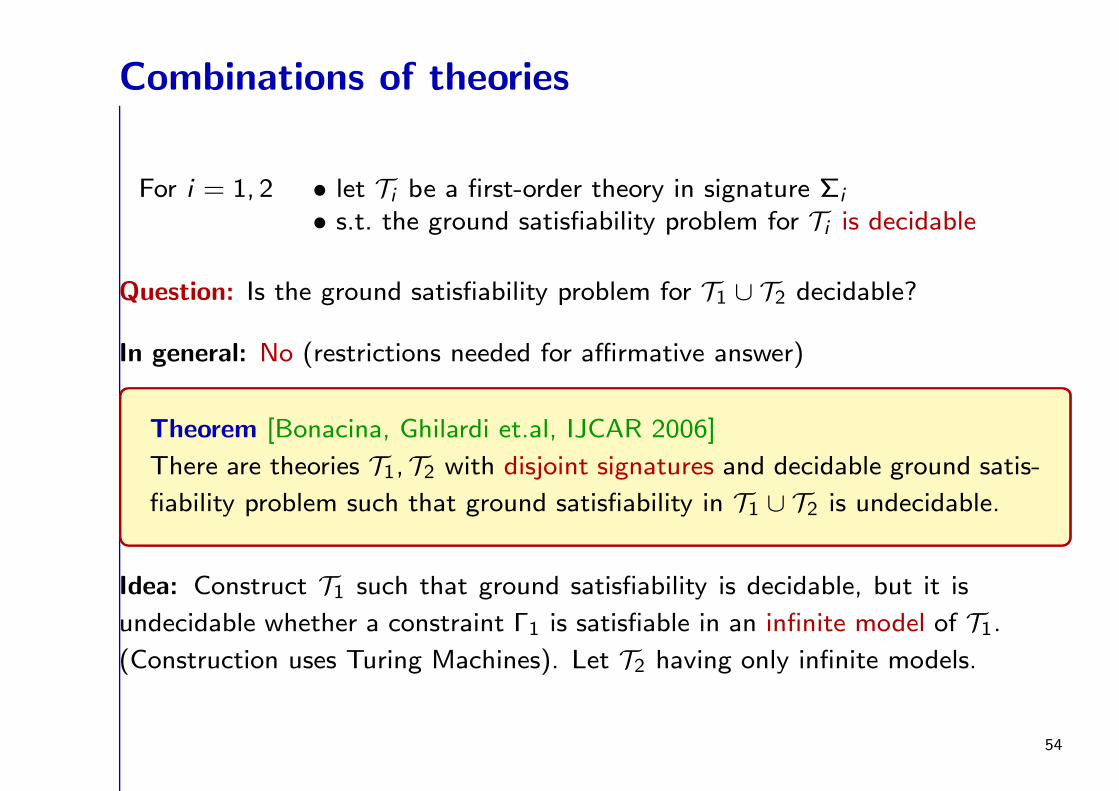
Combinations of theories
For i = 1, 2 • let Ti be a first-order theory in signature Σi
• s.t. the ground satisfiability problem for Ti is decidable
Question: Is the ground satisfiability problem for T1 ∪ T2 decidable?
In general: No (restrictions needed for affirmative answer)
Theorem [Bonacina, Ghilardi et.al, IJCAR 2006]
There are theories T1, T2 with disjoint signatures and decidable ground satis-
fiability problem such that ground satisfiability in T1 ∪ T2 is undecidable.
Idea: Construct T1 such that ground satisfiability is decidable, but it is
undecidable whether a constraint Γ1 is satisfiable in an infinite model of T1.
(Construction uses Turing Machines). Let T2 having only infinite models.
54
Combination of theories over disjoint signatures
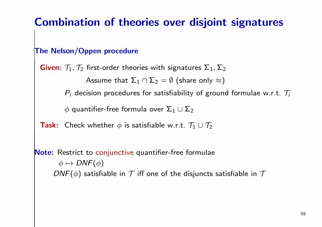
The Nelson/Oppen procedure
Given: T1, T2 first-order theories with signatures Σ1, Σ2
Assume that Σ1 ∩ Σ2 = ∅ (share only ≈)
Pi decision procedures for satisfiability of ground formulae w.r.t. Ti
φ quantifier-free formula over Σ1 ∪ Σ2
Task: Check whether φ is satisfiable w.r.t. T1 ∪ T2
Note: Restrict to conjunctive quantifier-free formulae
φ 7→ DNF (φ)
DNF (φ) satisfiable in T iff one of the disjuncts satisfiable in T
55
Example
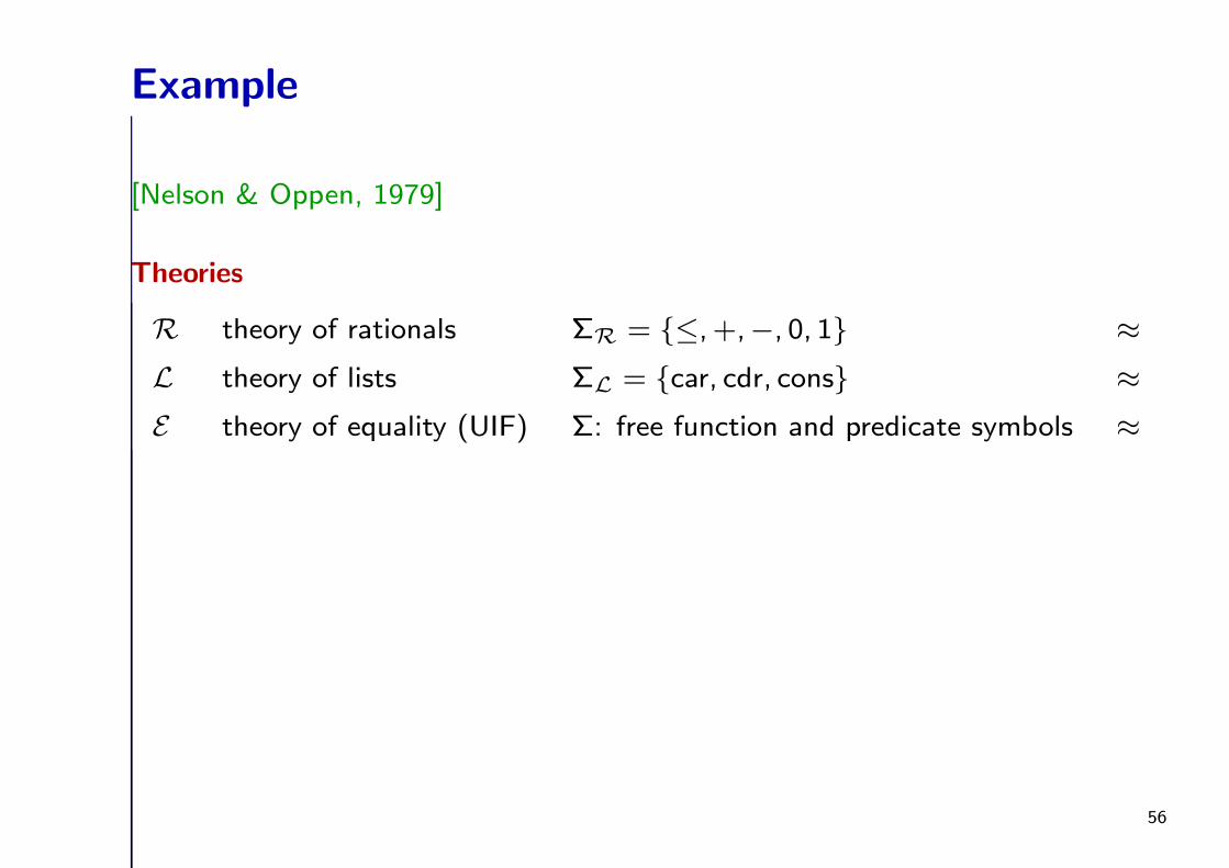
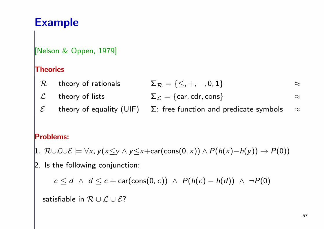
[Nelson & Oppen, 1979]
Theories
R theory of rationals ΣR = ≤, +,−, 0, 1 ≈
L theory of lists ΣL = car, cdr, cons ≈
E theory of equality (UIF) Σ: free function and predicate symbols ≈
56
Example
[Nelson & Oppen, 1979]
Theories
R theory of rationals ΣR = ≤, +,−, 0, 1 ≈
L theory of lists ΣL = car, cdr, cons ≈
E theory of equality (UIF) Σ: free function and predicate symbols ≈
Problems:
1. R∪L∪E |= ∀x , y(x≤y ∧ y≤x+car(cons(0, x)) ∧ P(h(x)−h(y)) → P(0))
2. Is the following conjunction:
c ≤ d ∧ d ≤ c + car(cons(0, c)) ∧ P(h(c)− h(d)) ∧ ¬P(0)
satisfiable in R∪ L ∪ E?
57
An Example
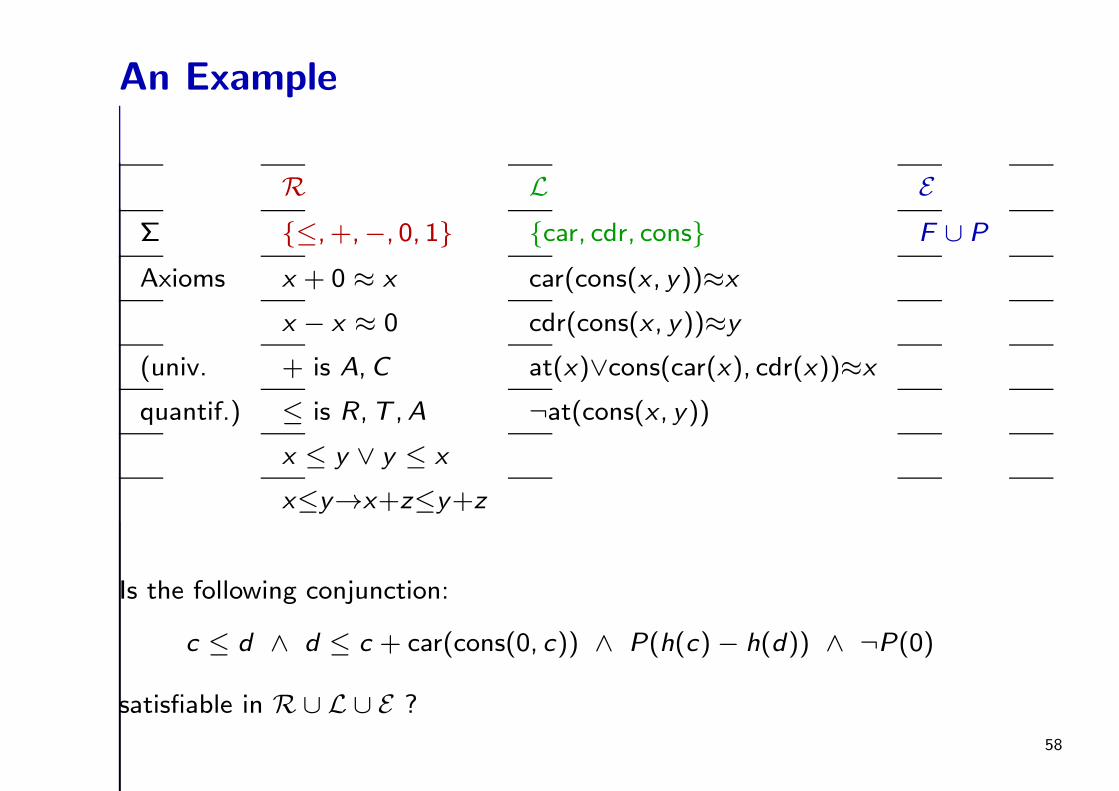
R L E
Σ ≤, +,−, 0, 1 car, cdr, cons F ∪ P
Axioms x + 0 ≈ x car(cons(x , y))≈x
x − x ≈ 0 cdr(cons(x , y))≈y
(univ. + is A,C at(x)∨cons(car(x), cdr(x))≈x
quantif.) ≤ is R,T ,A ¬at(cons(x , y))
x ≤ y ∨ y ≤ x
x≤y→x+z≤y+z
Is the following conjunction:
c ≤ d ∧ d ≤ c + car(cons(0, c)) ∧ P(h(c)− h(d)) ∧ ¬P(0)
satisfiable in R∪ L ∪ E ?
58
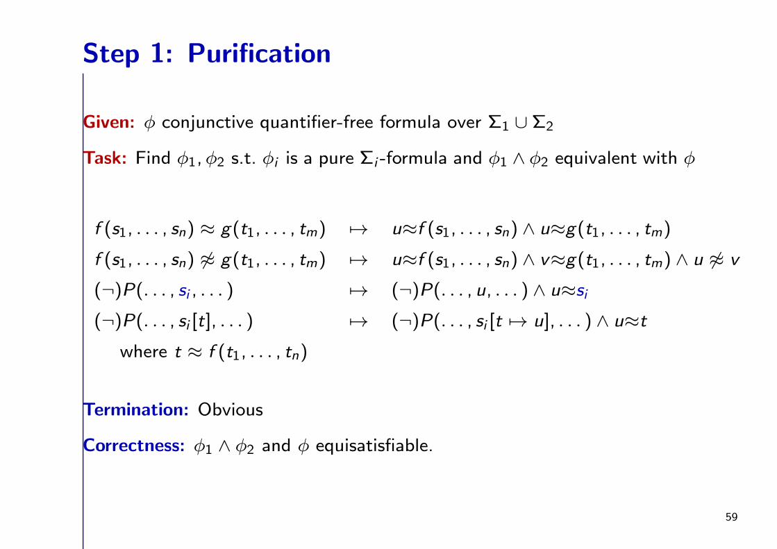
Step 1: Purification
Given: φ conjunctive quantifier-free formula over Σ1 ∪ Σ2
Task: Find φ1,φ2 s.t. φi is a pure Σi -formula and φ1 ∧ φ2 equivalent with φ
f (s1, . . . , sn) ≈ g(t1, . . . , tm) 7→ u≈f (s1, . . . , sn) ∧ u≈g(t1, . . . , tm)
f (s1, . . . , sn) 6≈ g(t1, . . . , tm) 7→ u≈f (s1, . . . , sn) ∧ v≈g(t1, . . . , tm) ∧ u 6≈ v
(¬)P(. . . , si , . . . ) 7→ (¬)P(. . . , u, . . . ) ∧ u≈si
(¬)P(. . . , si [t], . . . ) 7→ (¬)P(. . . , si [t 7→ u], . . . ) ∧ u≈t
where t ≈ f (t1, . . . , tn)
Termination: Obvious
Correctness: φ1 ∧ φ2 and φ equisatisfiable.
59
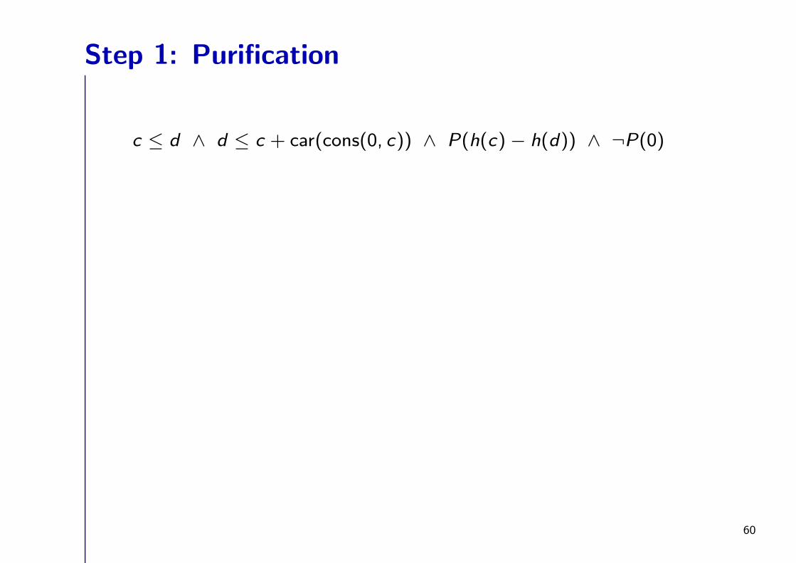
Step 1: Purification
c ≤ d ∧ d ≤ c + car(cons(0, c)) ∧ P(h(c)− h(d)) ∧ ¬P(0)
60
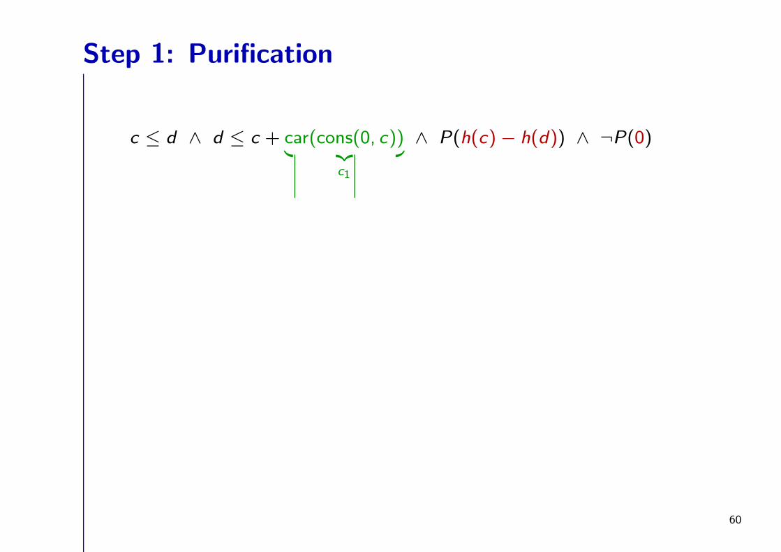
Step 1: Purification
c ≤ d ∧ d ≤ c + car(cons(0, c))︸ ︷︷ ︸
c1
∧ P(h(c)− h(d)) ∧ ¬P(0)
60
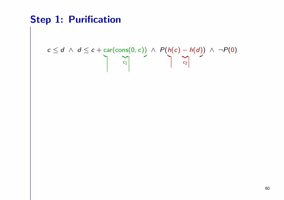
Step 1: Purification
c ≤ d ∧ d ≤ c + car(cons(0, c))︸ ︷︷ ︸
c1
∧ P(h(c)− h(d)︸ ︷︷ ︸
c2
) ∧ ¬P(0)
60
Step 1: Purification
c ≤ d ∧ d ≤ c + car(cons(0, c))︸ ︷︷ ︸
c1
∧ P(h(c)︸︷︷︸
c3
− h(d)︸︷︷︸
c4︸ ︷︷ ︸
c2
) ∧ ¬P( 0︸︷︷︸
c5
)
60
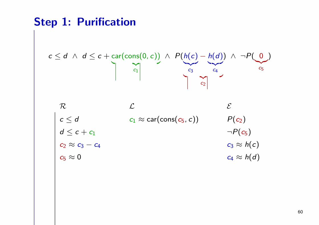
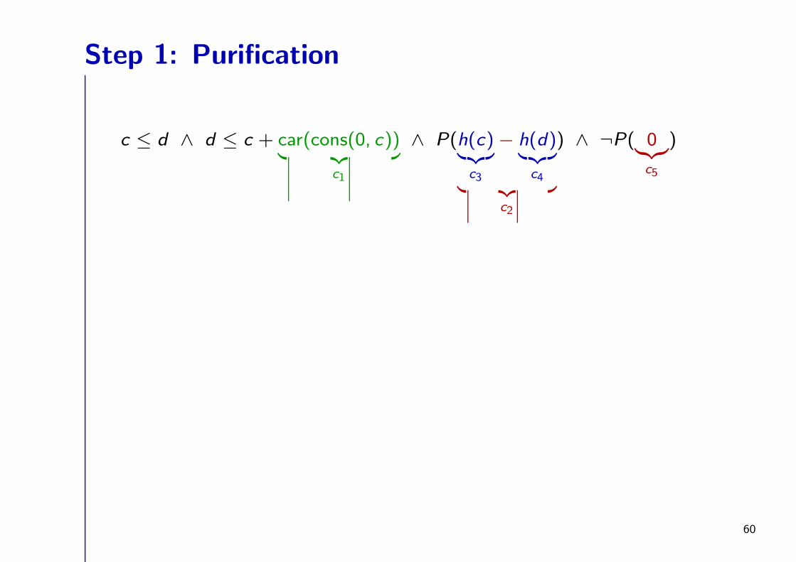
Step 1: Purification
c ≤ d ∧ d ≤ c + car(cons(0, c))︸ ︷︷ ︸
c1
∧ P(h(c)︸︷︷︸
c3
− h(d)︸︷︷︸
c4︸ ︷︷ ︸
c2
) ∧ ¬P( 0︸︷︷︸
c5
)
R L E
c ≤ d c1 ≈ car(cons(c5, c)) P(c2)
d ≤ c + c1 ¬P(c5)
c2 ≈ c3 − c4 c3 ≈ h(c)
c5 ≈ 0 c4 ≈ h(d)
60
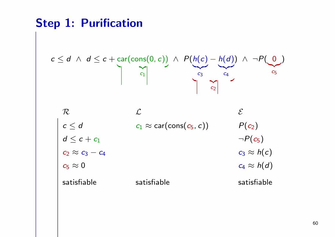
Step 1: Purification
c ≤ d ∧ d ≤ c + car(cons(0, c))︸ ︷︷ ︸
c1
∧ P(h(c)︸︷︷︸
c3
− h(d)︸︷︷︸
c4︸ ︷︷ ︸
c2
) ∧ ¬P( 0︸︷︷︸
c5
)
R L E
c ≤ d c1 ≈ car(cons(c5, c)) P(c2)
d ≤ c + c1 ¬P(c5)
c2 ≈ c3 − c4 c3 ≈ h(c)
c5 ≈ 0 c4 ≈ h(d)
satisfiable satisfiable satisfiable
60
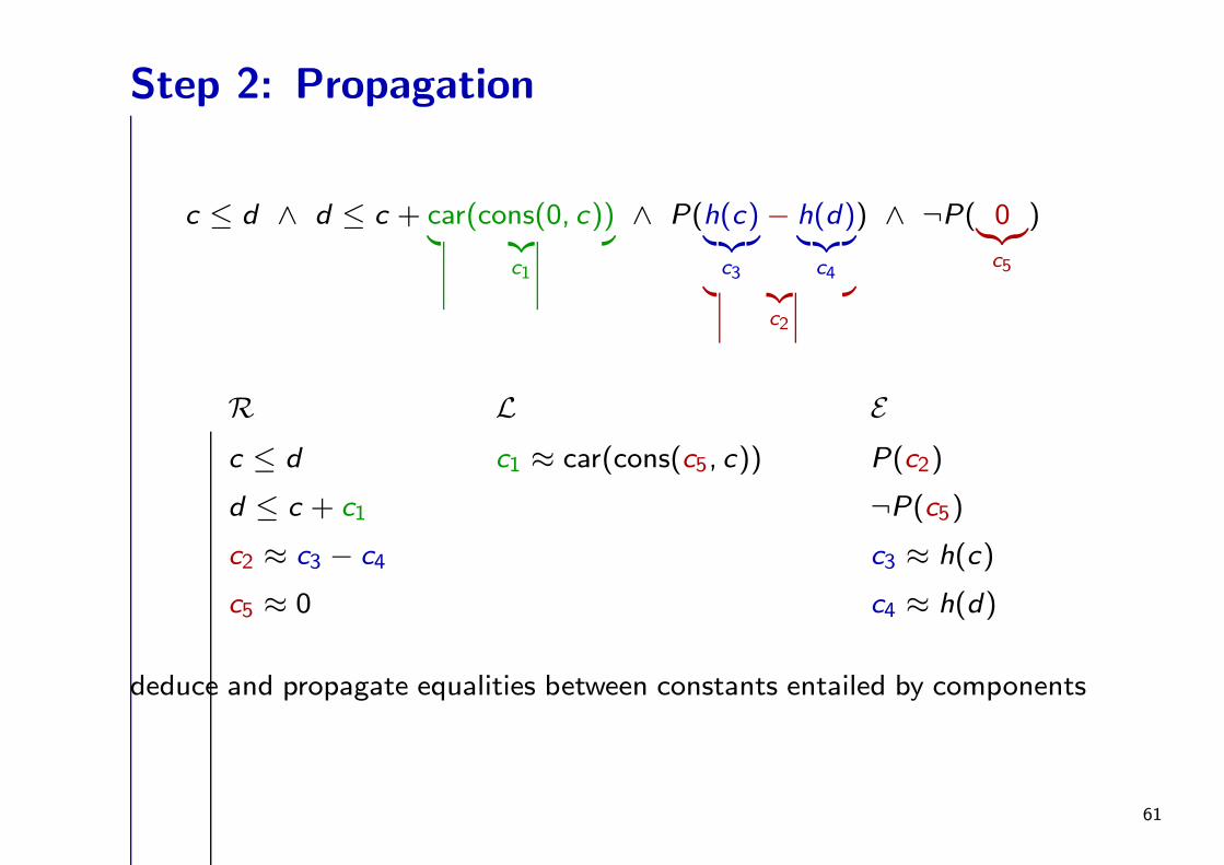
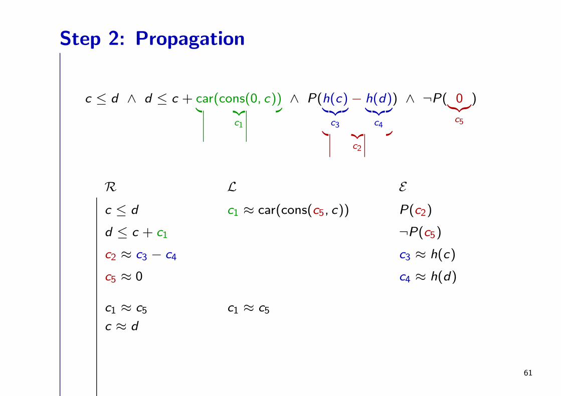
Step 2: Propagation
c ≤ d ∧ d ≤ c + car(cons(0, c))︸ ︷︷ ︸
c1
∧ P(h(c)︸︷︷︸
c3
− h(d)︸︷︷︸
c4︸ ︷︷ ︸
c2
) ∧ ¬P( 0︸︷︷︸
c5
)
R L E
c ≤ d c1 ≈ car(cons(c5, c)) P(c2)
d ≤ c + c1 ¬P(c5)
c2 ≈ c3 − c4 c3 ≈ h(c)
c5 ≈ 0 c4 ≈ h(d)
deduce and propagate equalities between constants entailed by components
61
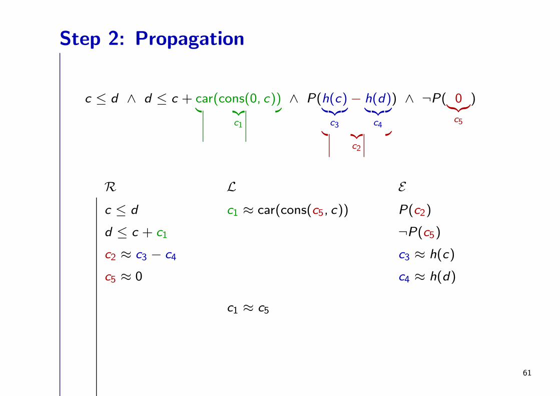
Step 2: Propagation
c ≤ d ∧ d ≤ c + car(cons(0, c))︸ ︷︷ ︸
c1
∧ P(h(c)︸︷︷︸
c3
− h(d)︸︷︷︸
c4︸ ︷︷ ︸
c2
) ∧ ¬P( 0︸︷︷︸
c5
)
R L E
c ≤ d c1 ≈ car(cons(c5, c)) P(c2)
d ≤ c + c1 ¬P(c5)
c2 ≈ c3 − c4 c3 ≈ h(c)
c5 ≈ 0 c4 ≈ h(d)
c1 ≈ c5
61
Step 2: Propagation
c ≤ d ∧ d ≤ c + car(cons(0, c))︸ ︷︷ ︸
c1
∧ P(h(c)︸︷︷︸
c3
− h(d)︸︷︷︸
c4︸ ︷︷ ︸
c2
) ∧ ¬P( 0︸︷︷︸
c5
)
R L E
c ≤ d c1 ≈ car(cons(c5, c)) P(c2)
d ≤ c + c1 ¬P(c5)
c2 ≈ c3 − c4 c3 ≈ h(c)
c5 ≈ 0 c4 ≈ h(d)
c1 ≈ c5 c1 ≈ c5
c ≈ d
61
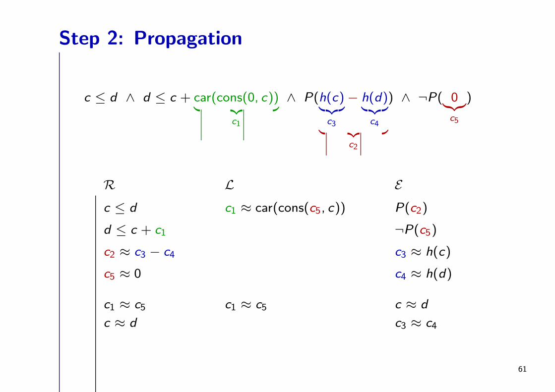
Step 2: Propagation
c ≤ d ∧ d ≤ c + car(cons(0, c))︸ ︷︷ ︸
c1
∧ P(h(c)︸︷︷︸
c3
− h(d)︸︷︷︸
c4︸ ︷︷ ︸
c2
) ∧ ¬P( 0︸︷︷︸
c5
)
R L E
c ≤ d c1 ≈ car(cons(c5, c)) P(c2)
d ≤ c + c1 ¬P(c5)
c2 ≈ c3 − c4 c3 ≈ h(c)
c5 ≈ 0 c4 ≈ h(d)
c1 ≈ c5 c1 ≈ c5 c ≈ d
c ≈ d c3 ≈ c4
61
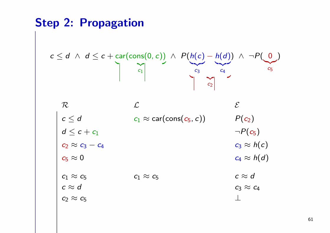
Step 2: Propagation
c ≤ d ∧ d ≤ c + car(cons(0, c))︸ ︷︷ ︸
c1
∧ P(h(c)︸︷︷︸
c3
− h(d)︸︷︷︸
c4︸ ︷︷ ︸
c2
) ∧ ¬P( 0︸︷︷︸
c5
)
R L E
c ≤ d c1 ≈ car(cons(c5, c)) P(c2)
d ≤ c + c1 ¬P(c5)
c2 ≈ c3 − c4 c3 ≈ h(c)
c5 ≈ 0 c4 ≈ h(d)
c1 ≈ c5 c1 ≈ c5 c ≈ d
c ≈ d c3 ≈ c4
c2 ≈ c5 ⊥
61
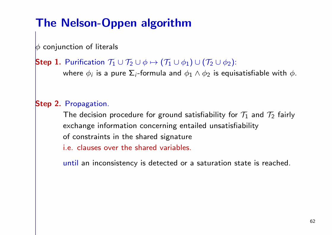
The Nelson-Oppen algorithm
φ conjunction of literals
Step 1. Purification T1 ∪ T2 ∪ φ 7→ (T1 ∪ φ1) ∪ (T2 ∪ φ2):
where φi is a pure Σi -formula and φ1 ∧ φ2 is equisatisfiable with φ.
Step 2. Propagation.
The decision procedure for ground satisfiability for T1 and T2 fairly
exchange information concerning entailed unsatisfiability
of constraints in the shared signature
i.e. clauses over the shared variables.
until an inconsistency is detected or a saturation state is reached.
62
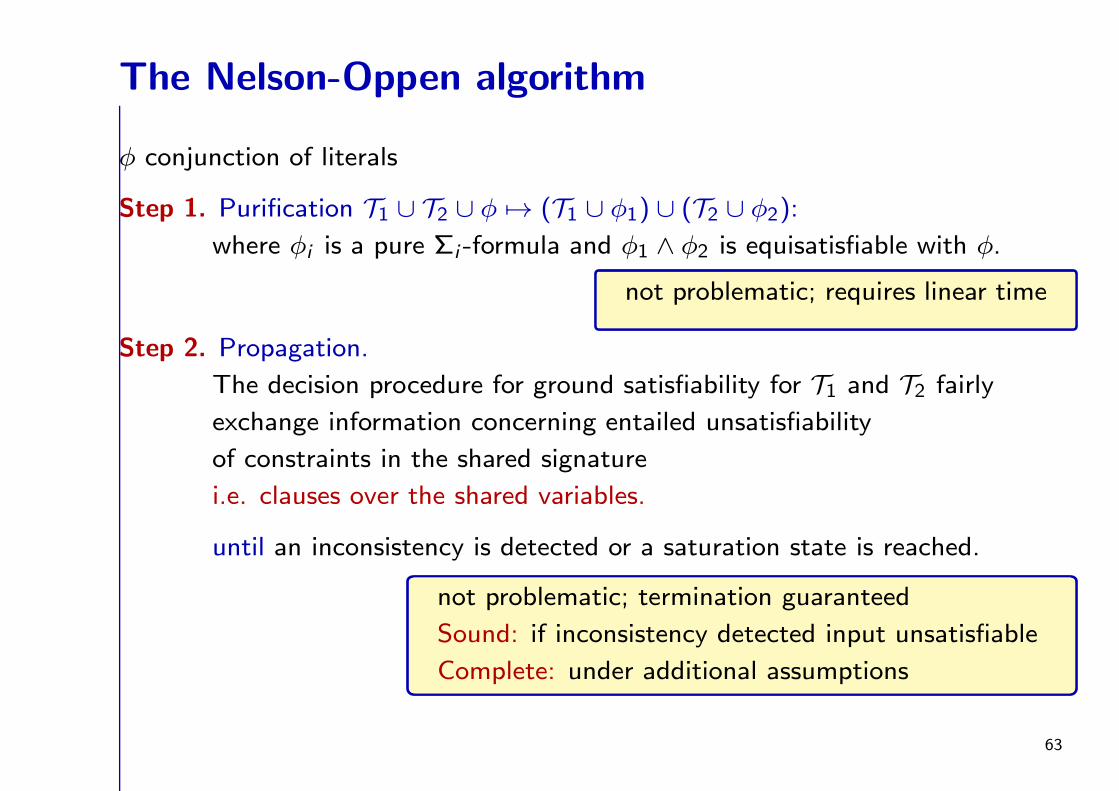
The Nelson-Oppen algorithm
φ conjunction of literals
Step 1. Purification T1 ∪ T2 ∪ φ 7→ (T1 ∪ φ1) ∪ (T2 ∪ φ2):
where φi is a pure Σi -formula and φ1 ∧ φ2 is equisatisfiable with φ.
Step 2. Propagation.
The decision procedure for ground satisfiability for T1 and T2 fairly
exchange information concerning entailed unsatisfiability
of constraints in the shared signature
i.e. clauses over the shared variables.
until an inconsistency is detected or a saturation state is reached.
not problematic; requires linear time
not problematic; termination guaranteed
Sound: if inconsistency detected input unsatisfiable
Complete: under additional assumptions
63