Archives of Control Sciences, Vol. 6 (XLII), 1997, No. 1-2, pp. 5-27.

Decision Making Under Ambiguity: A Belief-Function Perspective

Rajendra P. Srivastava* Ernst & Young Professor

Director, Ernst & Young Center for Auditing Research and Advanced Technology

Division of Accounting and Information Systems School of Business, The University of Kansas

Lawrence, KS 66045, USA

*The author would like to thank Mike Ettredge, Peter Gillett, Theodore Mock, Steven Salterio, and Prakash Shenoy for their insightful comments on the paper. Also, the author sincerely appreciates the helpful comments provided by the AI workshop participants at the University of Kansas.

1

Decision Making Under Ambiguity: A Belief-Function Perspective

ABSTRACT

In this article, we discuss problems with probability theory in representing uncertainties

encountered in the "real world" and show how belief functions can overcome these difficulties.

Also, we discuss an expected utility approach of decision making under ambiguity using the

belief function framework. In particular, we develop a proposition for decision making under

ambiguity using the expected utility theory. This proposition is based on Strat�s approach of

resolving ambiguity in the problem using belief functions. We use the proposition to explain the

Ellsberg paradox and model the decision making behavior under ambiguity. We use the

empirical data of Einhorn and Hogarth to validate the proposition. Also, we use the proposition

to predict several decision making behaviors under ambiguity for special conditions.

Furthermore, we discuss the general condition under which the �switching� behavior, as

observed by Einhorn and Hogarth, will occur using the concept of �precision measure� in the

expected utility theory.

2

Decision Making Under Ambiguity: A Belief-Function Perspective

1. INTRODUCTION

This article has four objectives. As the first objective, we discuss problems with proba-

bilities in representing uncertainties encountered on real decisions and then show how belief

functions (Shafer, 1976) provide a better framework than probabilities to represent such

uncertainties. As the second objective, we develop a proposition for decision making under

ambiguity, represented in terms of belief functions, using Strat�s (1990, 1994) approach. As the

third objective, we explain Ellsberg�s paradox (1961) using the proposition and validate it using

the empirical data of Einhorn and Hogarth (1986, hereafter called EH).

It is a well known fact that probability theory is unable to distinguish between a situation

of complete ignorance and a situation where we have complete knowledge. In fact, as discussed

in Section 2.2, Ellsberg�s paradox stems from this inability of probability theory. There are many

real world situations such as auditing or medical diagnosis where the decision maker is not able

to easily represent uncertainties using probabilities. We show in this article how belief functions

provide a better framework to represent such uncertainties than probabilities.

In general, the expected utility approach under the belief-function framework gives an

interval for the expected value instead of a single estimate. In fact, this has been the major

hurdle of using the traditional decision theory in the belief-function framework. Recently,

several approaches to decision making under the belief-function framework have been proposed

(see, i.e., Jaffray, 1989, 1994; Nguyen and Walker, 1994; Smets, 1990a, 1990b; Strat, 1990,

1994; and Yager, 1990 for details). We use1 Strat�s approach (1990, 1994) to develop a

proposition for decision making under ambiguity. In essence, this proposition suggests that the

decision maker (hereafter called DM) will take a conservative approach and make the decision

based on the most unfavorable resolution of ambiguity. Under the above scheme, if there is no

clear choice, then he or she will make the decision based on the most favorable resolution of

3

ambiguity. This rule is equivalent to �minimax� rule in a two-person zero-sum game. It is

interesting to note that the proposition developed in the article not only explains Ellsberg�s

paradox but also models correctly all the behaviors observed by EH.

The remaining article is divided into six sections. Section 2 discusses the issues related

to Ellsberg�s paradox, and shows the problems with probability theory in modeling uncertainties

encountered in the real world. Section 3 presents an introduction to belief functions. Section 4

presents the expected utility approach to decision making under probabilities, and belief

functions. A proposition for decision making under ambiguity is developed in Section 5. Also,

the �switching� behavior, as observed by EH, is discussed in Section 5. Section 6 validates the

proposition using the EH empirical results. Finally, Section 7 presents summary and conclusions

of the study.

2. ELLSBERG PARADOX AND PROBLEMS WITH PROBABILITY

2.1 Ellsberg Paradox

Einhorn and Hogarth (1986) conducted an experiment where the subjects were asked to

imagine two urns. Urn 1 contained 100 balls with unknown proportions of black and red. Urn 2

contained 50 red balls and 50 black balls. The subjects were asked to play a gamble and win

$100 if they picked a ball of specified color (red or black) from one of the urns. If a wrong ball

was picked then the payoff was $0. Most of the subjects preferred to pick from Urn 2 (non-

ambiguous). If one tries to explain the above experimental result using probability theory he or

she runs into a paradox. Such a paradox is known as the Ellsberg paradox (1961). Here is an

argument provided by EH (1986, pp. S227-228) using probability theory to illustrate the paradox.

In case of Urn 1, we have a completely unknown situation, i.e., we are completely igno-

rant about how many red or black balls there are. In such an ignorant situation, the probability

theory tells us to assign equal probability to all the possible mutually exclusive and exhaustive

states. Under such an assumption, we find that the probability of picking a red ball from Urn 1 is

P(R1) = 0.5 and so is the probability of picking a black ball, i.e., P(B1) = 0.5. In case of Urn 2,

4

we know that it contains 50 red and 50 black balls which implies that the probabilities of picking

a red or a black ball, respectively, are: P(R2) = 0.5 and P(B2) = 0.5. As EH discuss, the prefer-

ence of Urn 2 over Urn 1 for picking a ball of either color would mean that

P(R2) > P(R1) = 0.5, P(B2) > P(B1) = 0.5,

or

P(R2) = 0.5 > P(R1), P(B2) = 0.5 > P(B1).

The first condition implies that the probabilities for Urn 2 add to more than one and the second

condition implies that the probabilities for Urn 1 add to less than one. This is the paradox. EH

define these conditions, respectively, as "superadditivity" and "subadditivity." They further com-

ment that (Einhorn and Hogarth 1986, p. S228):

... either urn 2 has complementary probabilities that sum to more than one, or urn 1 has complementary probabilities that sum to less than one. As we will show, the nonadditivity of complementary probabilities is central to judgments under ambiguity.

However, we show that no such super- or sub-additivity is needed to explain the decision

maker's behavior if we use a belief functions treatment of ambiguity. The paradox stems from

the difficulties we face in representing ignorance using probabilities. Under probability theory,

the above two situations are treated in exactly the same manner. However, decision makers

clearly perceive the situations to be different. We show in this article that really there is no

paradox if we model the uncertainties properly, i.e., using the belief-function framework.

2.2 Problems with Probability

We will not present a philosophical discussion about the concept of probability and

objective versus subjective probabilities. This has been done several times and it has been an

ongoing process (see, e.g., Schoemaker, 1982; and Shafer, 1976). Instead, we give some real

world situations where probability concepts are not adequate to model the feelings of the DMs

about uncertainties.

5

Let us first consider the studies in behavioral decision theory. There are several studies

that have demonstrated the problems of representing human judgment about uncertainties using

probabilities (see, e.g., Einhorn and Hogarth, 1985, 1986; Kahneman, Slovic, and Tversky, 1982;

Kahneman and Tversky, 1979; and Tversky and Kahneman, 1986). Just to reemphasize the

point, we reconsider the famous Ellsberg paradox presented earlier. It is clear that we are not

able to distinguish between a state of complete ignorance (Urn 1 with unknown proportions of

red and black balls) and a state of complete knowledge (Urn 2 with 50 red balls and 50 black

balls) when we use probability theory to model uncertainties involved in the two cases.

Let us consider another situation, an example in auditing. Auditors have to deal with un-

certain items of evidence on every engagement. But the uncertainties associated with such items

of evidence and the auditor's feeling or judgment about these uncertainties cannot be modeled

easily using the concepts of probability. For example, auditors use analytical procedures such as

ratios, projections, time series analysis, and linear regression to compare the numbers thus

computed with the recorded account balances in the company's books. If the computed figure is

reasonably close to the recorded account balance, then the auditor considers the recorded balance

to be fairly stated. But he or she cannot put a high level of assurance that the balance is fairly

stated just on the basis of projections and ratio analyses, because there could be several other

reasons that the balance is close to the calculated figure when in reality it contains errors.

Suppose the auditor has a positive feeling about the recorded balance based on the

analytical procedures, since the projection is close to the recorded balance. Suppose also that the

economic environment has been almost the same as in the previous periods. That is, there is no

reason to expect that the recorded balance should be any different from the projected one. The

auditor wants to assign a positive, but low, level of support from this item of evidence that the

account is fairly stated. Let us say that the auditor assigns a low level of support, say 0.3 on a

scale of 0-1, to the state that the account balance is fairly stated based on this evidence alone.

The question is, what is this number 0.3 and what happens to the remaining 0.7? If we interpret

these numbers as probabilities, then we at once conclude that the auditor is saying he or she has

6

0.7 degree of confidence that the account is not fairly stated. But this is not what the auditor has

in mind. Shafer and Srivastava (1990), Srivastava (1993), and Srivastava and Shafer (1992) have

argued that belief-function theory provides a better framework for audit decisions.

Moreover, there are several studies in AI (Artificial Intelligence) that focus on modeling

human decision making and have found probabilities to be inadequate in modeling uncertainties

encountered on real decisions. Davis, Buchanan, and Shortliffe (1977) developed MYCIN to

diagnose the common cold. They were unable to use probability framework to model

uncertainties encountered in making this real decision. They used instead a certainty factor with

ad hoc rules to combine them in their system but acknowledged the need for a normative theory

to deal with their situation. They also acknowledged that the Dempster-Shafer theory of belief

functions seems to have some promise in managing the kinds of uncertainties they were facing.

There are several frameworks that have been proposed to model uncertainties of the kind

discussed above: Zadeh's fuzzy set theory (1965), Dubois and Prade's possibility and necessity

theory (1987, 1990), and Dempster-Shafer theory of belief functions (Shafer, 1976). We focus

on the Dempster-Shafer theory of belief functions in the current article.

3. BELIEF FUNCTIONS AND AMBIGUITY

The basic concepts of belief functions2 have appeared in several places. Of course, A

Mathematical Theory of Evidence by Shafer (1976) provides the most comprehensive coverage

on the subject. The current form of the belief-function formalism, known as Dempster-Shafer

theory of belief functions, is the works of Dempster in the 1960's and of Shafer in the 1970's. In

this article, we will give only the basics of belief functions. Since the present paper does not deal

with the combination of evidence, we will not give Dempster's rule of combination. Interested

readers should see Shafer (1976) for details.

The basic difference between probability theory and the belief-function formalism is in

the assignment of uncertainties to a set of mutually exclusive and exhaustive states or assertions

under consideration (we will call this set a frame and represent it by the symbol Θ). In

7

probability theory, we assign uncertainty to each individual element of the frame and call it the

probability of occurrence of the element. The sum of all these probabilities equals one.

Let us consider an auditing example. The accounts receivable balance is not materially

misstated (ar) and it is materially misstated (~ar) are the two assertions representing a mutually

exclusive and exhaustive set. Here the frame consists of the two elements3: Θ = {ar, ~ar}. In

probability theory, we will assign probability to each element of the frame, i.e., P(ar) ≥ 0, and

P(~ar) ≥ 0. Also, we know that P(ar) + P(~ar) = 1. In the belief-function framework, uncertainty

is not only assigned to the single elements of the frame but also to all other proper subsets of the

frame and to the entire frame. We call these uncertainties m-values or the basic probability

assignment function.

3.1 m-values (The Basic Probability Assignment Function)

Similar to probabilities, all these m-values add to one. For the example considered

above4, we will have m(ar) ≥ 0, m(~ar) ≥ 0, m({ar, ~ar}) ≥ 0, and m(ar) + m(~ar) + m({ar, ~ar})

= 1. Let us assume that the auditor has performed analytical procedures, as discussed in the

introduction, relevant to the accounts receivable balance and finds no significant difference

between the recorded value and the predicted value. Based on this finding, he or she feels that

the recorded value appears reasonable and is not materially misstated. However, he or she does

not want to put too much weight on this evidence. He/she feels he/she can assign a small level of

assurance, say 0.3 on a scale of 0-1, that the account is not materially misstated. We can express

this feeling in terms of m-values as: m(ar) = 0.3, m(~ar) = 0, and m({ar, ~ar}) = 0.7. The belief

function interpretation of these m-values is that the auditor has 0.3 level of support to 'ar', no

support to '~ar', and 0.7 level of support remains uncommitted which represents ignorance.

However, if we had to express the above feelings in terms of probabilities, then we get

into problems, because we will assign P(ar) = 0.3 and P(~ar) = 0.7 which implies that there is a

70 percent chance that the account is materially misstated, but we know that this is not what the

auditor is trying to say. The auditor has no reason to believe that the account is materially

8

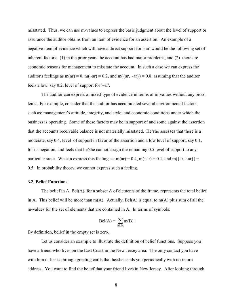
misstated. Thus, we can use m-values to express the basic judgment about the level of support or

assurance the auditor obtains from an item of evidence for an assertion. An example of a

negative item of evidence which will have a direct support for '~ar' would be the following set of

inherent factors: (1) in the prior years the account has had major problems, and (2) there are

economic reasons for management to misstate the account. In such a case we can express the

auditor's feelings as m(ar) = 0, m(~ar) = 0.2, and m({ar, ~ar}) = 0.8, assuming that the auditor

feels a low, say 0.2, level of support for '~ar'.

The auditor can express a mixed-type of evidence in terms of m-values without any prob-

lems. For example, consider that the auditor has accumulated several environmental factors,

such as: management�s attitude, integrity, and style; and economic conditions under which the

business is operating. Some of these factors may be in support of and some against the assertion

that the accounts receivable balance is not materially misstated. He/she assesses that there is a

moderate, say 0.4, level of support in favor of the assertion and a low level of support, say 0.1,

for its negation, and feels that he/she cannot assign the remaining 0.5 level of support to any

particular state. We can express this feeling as: m(ar) = 0.4, m(~ar) = 0.1, and m({ar, ~ar}) =

0.5. In probability theory, we cannot express such a feeling.

3.2 Belief Functions

The belief in A, Bel(A), for a subset A of elements of the frame, represents the total belief

in A. This belief will be more than m(A). Actually, Bel(A) is equal to m(A) plus sum of all the

m-values for the set of elements that are contained in A. In terms of symbols:

Bel(A) = m(B)B A⊆∑ .

By definition, belief in the empty set is zero.

Let us consider an example to illustrate the definition of belief functions. Suppose you

have a friend who lives on the East Coast in the New Jersey area. The only contact you have

with him or her is through greeting cards that he/she sends you periodically with no return

address. You want to find the belief that your friend lives in New Jersey. After looking through

9

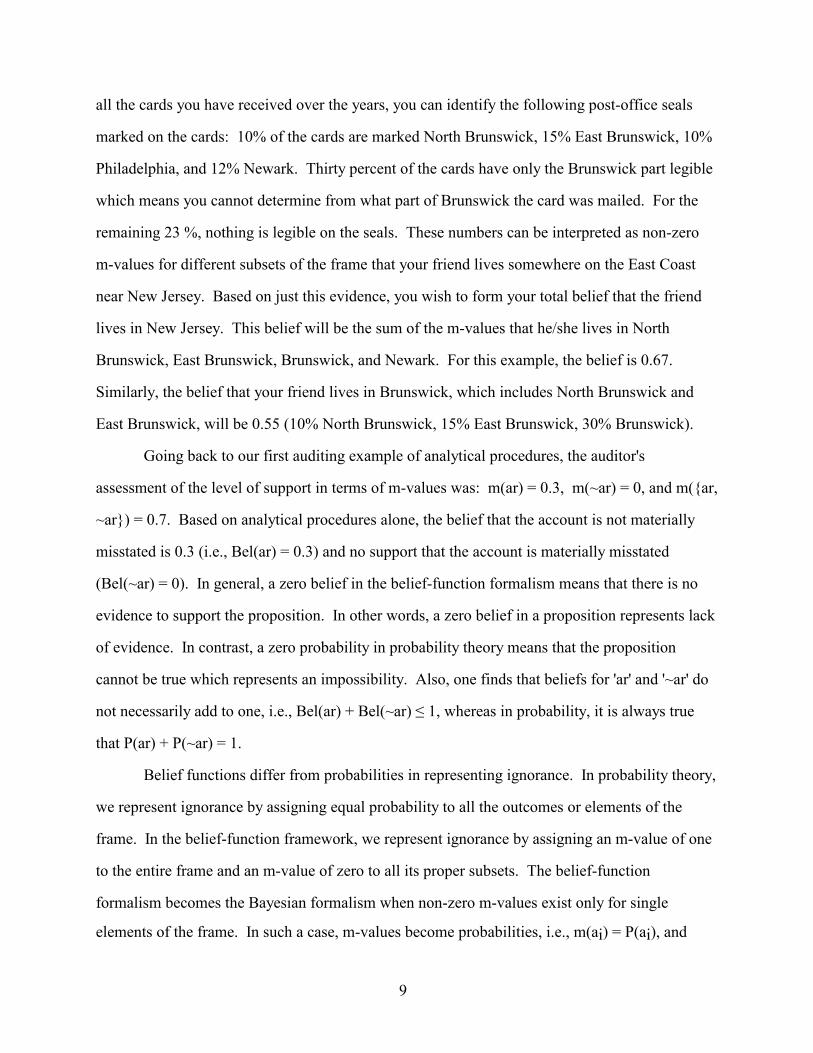
all the cards you have received over the years, you can identify the following post-office seals

marked on the cards: 10% of the cards are marked North Brunswick, 15% East Brunswick, 10%

Philadelphia, and 12% Newark. Thirty percent of the cards have only the Brunswick part legible

which means you cannot determine from what part of Brunswick the card was mailed. For the

remaining 23 %, nothing is legible on the seals. These numbers can be interpreted as non-zero

m-values for different subsets of the frame that your friend lives somewhere on the East Coast

near New Jersey. Based on just this evidence, you wish to form your total belief that the friend

lives in New Jersey. This belief will be the sum of the m-values that he/she lives in North

Brunswick, East Brunswick, Brunswick, and Newark. For this example, the belief is 0.67.

Similarly, the belief that your friend lives in Brunswick, which includes North Brunswick and

East Brunswick, will be 0.55 (10% North Brunswick, 15% East Brunswick, 30% Brunswick).

Going back to our first auditing example of analytical procedures, the auditor's

assessment of the level of support in terms of m-values was: m(ar) = 0.3, m(~ar) = 0, and m({ar,

~ar}) = 0.7. Based on analytical procedures alone, the belief that the account is not materially

misstated is 0.3 (i.e., Bel(ar) = 0.3) and no support that the account is materially misstated

(Bel(~ar) = 0). In general, a zero belief in the belief-function formalism means that there is no

evidence to support the proposition. In other words, a zero belief in a proposition represents lack

of evidence. In contrast, a zero probability in probability theory means that the proposition

cannot be true which represents an impossibility. Also, one finds that beliefs for 'ar' and '~ar' do

not necessarily add to one, i.e., Bel(ar) + Bel(~ar) ≤ 1, whereas in probability, it is always true

that P(ar) + P(~ar) = 1.

Belief functions differ from probabilities in representing ignorance. In probability theory,

we represent ignorance by assigning equal probability to all the outcomes or elements of the

frame. In the belief-function framework, we represent ignorance by assigning an m-value of one

to the entire frame and an m-value of zero to all its proper subsets. The belief-function

formalism becomes the Bayesian formalism when non-zero m-values exist only for single

elements of the frame. In such a case, m-values become probabilities, i.e., m(ai) = P(ai), and

10

Dempster's rule in the belief-function formalism becomes Bayes' rule in the probability theory

(Shafer, 1976).

3.3 Plausibility Functions

By definition, the plausibility of A is equal to one minus the belief in ~A, i.e., Pl(A) = 1 -

Bel(~A) where ~A represents the set of elements that are not in A. Intuitively, the plausibility of

A is the degree to which A is plausible given the evidence. In other words, Pl(A) is the degree to

which we do not assign belief to its negation ~A.

In our example of analytical procedures, we have Bel(ar) = 0.3, Bel(~ar) = 0. These val-

ues yield the following plausibility values: Pl(ar) = 1, and Pl(~ar) = 0.7. Pl(ar) = 1 indicates that

'ar' is maximally plausible since we have no evidence against it. However, Pl(~ar) = 0.7 indicates

that if we had no other items of evidence to consider then the maximum possible assurance that

the account is materially misstated would be 0.7, even though we have no evidence that the

account is materially misstated (Bel(~ar) = 0).

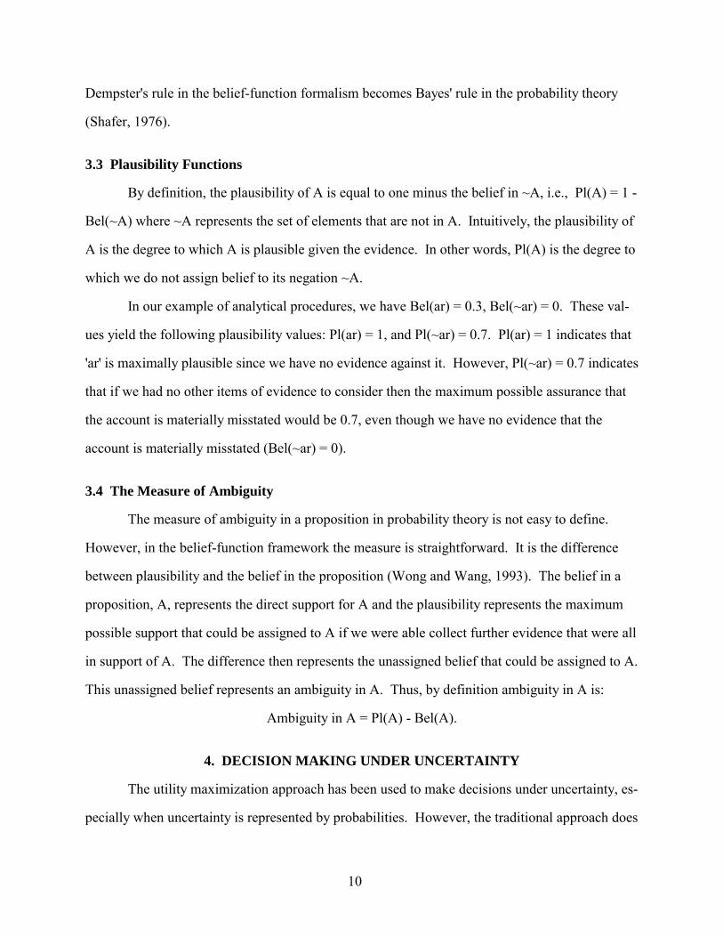
3.4 The Measure of Ambiguity

The measure of ambiguity in a proposition in probability theory is not easy to define.

However, in the belief-function framework the measure is straightforward. It is the difference

between plausibility and the belief in the proposition (Wong and Wang, 1993). The belief in a

proposition, A, represents the direct support for A and the plausibility represents the maximum

possible support that could be assigned to A if we were able collect further evidence that were all

in support of A. The difference then represents the unassigned belief that could be assigned to A.

This unassigned belief represents an ambiguity in A. Thus, by definition ambiguity in A is:

Ambiguity in A = Pl(A) - Bel(A).

4. DECISION MAKING UNDER UNCERTAINTY

The utility maximization approach has been used to make decisions under uncertainty, es-

pecially when uncertainty is represented by probabilities. However, the traditional approach does

11

not work when uncertainties are not represented by probabilities. In this paper, we illustrate

Strat�s approach (1990, 1994) of decision making when uncertainties are represented in terms of

belief functions. In order to illustrate the process, we first discuss the example given by Strat in

probability framework and change the situation and describe how the decision can be made using

belief functions.

4.1 Decision Making Using Probabilities

Consider Strat�s example of Carnival Wheel #1(Strat, 1994). This wheel has ten equal

sectors. Each sector is labeled with a dollar amount as follows. Four sectors are labeled $1,

three sectors $5, two $10, and one $20. The player gets to spin the wheel for a $6 fee and

receives the amount shown in the sector that stops at the top. The question is would you spin the

wheel?

In this example, we have four outcomes ($1, $5, $10, $20) and the related uncertainties

are represented by the following probability distribution:

P($1) = 0.4, P($5) = 0.3, P($10) = 0.2, and P($20) = 0.1.

The expected value of the game is:

E(x) = Σ xP(x) = 0.4($1) + 0.3($5) + 0.2($10) + 0.1($20) = $5.90

The expected values of utility is:

E(U(x)) = ΣP(x)U(x) = 0.4U($1) + 0.3U($5) + 0.2U($10) + 0.1U($20).

If one had to make a decision based on the expected value, then one would not play the game

since the expected value of the game ($5.90) is smaller that the ticket price ($6). Although not

presented here, we can argue that a rational individual with a risk averse attitude will reach the

same conclusion if he or she had to make the decision based on the utility maximization rule

(e.g., E(U(- $6)) < U($0)).

4.2 Decision Making Using Belief Functions

Let us consider a situation where uncertainties related to the random events in a decision

problem are not expressible in terms of probabilities but in terms of belief functions. As an

12

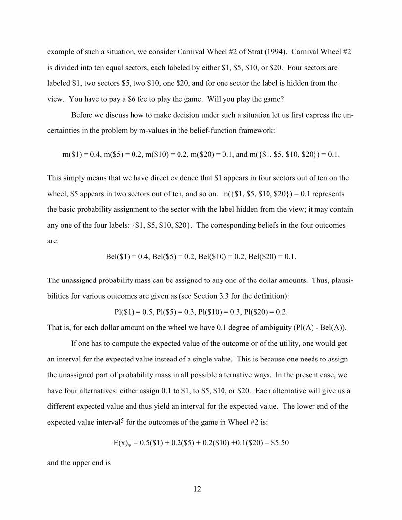
example of such a situation, we consider Carnival Wheel #2 of Strat (1994). Carnival Wheel #2

is divided into ten equal sectors, each labeled by either $1, $5, $10, or $20. Four sectors are

labeled $1, two sectors $5, two $10, one $20, and for one sector the label is hidden from the

view. You have to pay a $6 fee to play the game. Will you play the game?

Before we discuss how to make decision under such a situation let us first express the un-

certainties in the problem by m-values in the belief-function framework:

m($1) = 0.4, m($5) = 0.2, m($10) = 0.2, m($20) = 0.1, and m({$1, $5, $10, $20}) = 0.1.

This simply means that we have direct evidence that $1 appears in four sectors out of ten on the

wheel, $5 appears in two sectors out of ten, and so on. m({$1, $5, $10, $20}) = 0.1 represents

the basic probability assignment to the sector with the label hidden from the view; it may contain

any one of the four labels: {$1, $5, $10, $20}. The corresponding beliefs in the four outcomes

are:

Bel($1) = 0.4, Bel($5) = 0.2, Bel($10) = 0.2, Bel($20) = 0.1.

The unassigned probability mass can be assigned to any one of the dollar amounts. Thus, plausi-

bilities for various outcomes are given as (see Section 3.3 for the definition):

Pl($1) = 0.5, Pl($5) = 0.3, Pl($10) = 0.3, Pl($20) = 0.2.

That is, for each dollar amount on the wheel we have 0.1 degree of ambiguity (Pl(A) - Bel(A)).

If one has to compute the expected value of the outcome or of the utility, one would get

an interval for the expected value instead of a single value. This is because one needs to assign

the unassigned part of probability mass in all possible alternative ways. In the present case, we

have four alternatives: either assign 0.1 to $1, to $5, $10, or $20. Each alternative will give us a

different expected value and thus yield an interval for the expected value. The lower end of the

expected value interval5 for the outcomes of the game in Wheel #2 is:

E(x)* = 0.5($1) + 0.2($5) + 0.2($10) +0.1($20) = $5.50

and the upper end is

13

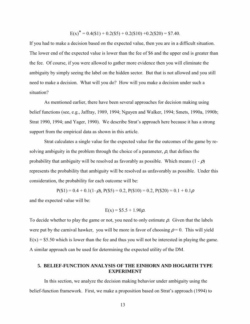
E(x)* = 0.4($1) + 0.2($5) + 0.2($10) +0.2($20) = $7.40.

If you had to make a decision based on the expected value, then you are in a difficult situation.

The lower end of the expected value is lower than the fee of $6 and the upper end is greater than

the fee. Of course, if you were allowed to gather more evidence then you will eliminate the

ambiguity by simply seeing the label on the hidden sector. But that is not allowed and you still

need to make a decision. What will you do? How will you make a decision under such a

situation?

As mentioned earlier, there have been several approaches for decision making using

belief functions (see, e.g., Jaffray, 1989, 1994; Nguyen and Walker, 1994; Smets, 1990a, 1990b;

Strat 1990, 1994; and Yager, 1990). We describe Strat�s approach here because it has a strong

support from the empirical data as shown in this article.

Strat calculates a single value for the expected value for the outcomes of the game by re-

solving ambiguity in the problem through the choice of a parameter, ρ, that defines the

probability that ambiguity will be resolved as favorably as possible. Which means (1 - ρ)

represents the probability that ambiguity will be resolved as unfavorably as possible. Under this

consideration, the probability for each outcome will be:

P($1) = 0.4 + 0.1(1�ρ), P($5) = 0.2, P($10) = 0.2, P($20) = 0.1 + 0.1ρ

and the expected value will be:

E(x) = $5.5 + 1.90ρ.

To decide whether to play the game or not, you need to only estimate ρ. Given that the labels

were put by the carnival hawker, you will be more in favor of choosing ρ = 0. This will yield

E(x) = $5.50 which is lower than the fee and thus you will not be interested in playing the game.

A similar approach can be used for determining the expected utility of the DM.

5. BELIEF-FUNCTION ANALYSIS OF THE EINHORN AND HOGARTH TYPE EXPERIMENT

In this section, we analyze the decision making behavior under ambiguity using the

belief-function framework. First, we make a proposition based on Strat�s approach (1994) to

14

decision making using belief functions. Next, we use the proposition to predict various observ-

able decision making behaviors in a general case of the EH type experiment with two urns. In

the next section, we show that Ellsberg�s result and the EH results are special cases of our

general results which follow directly from Proposition 1.

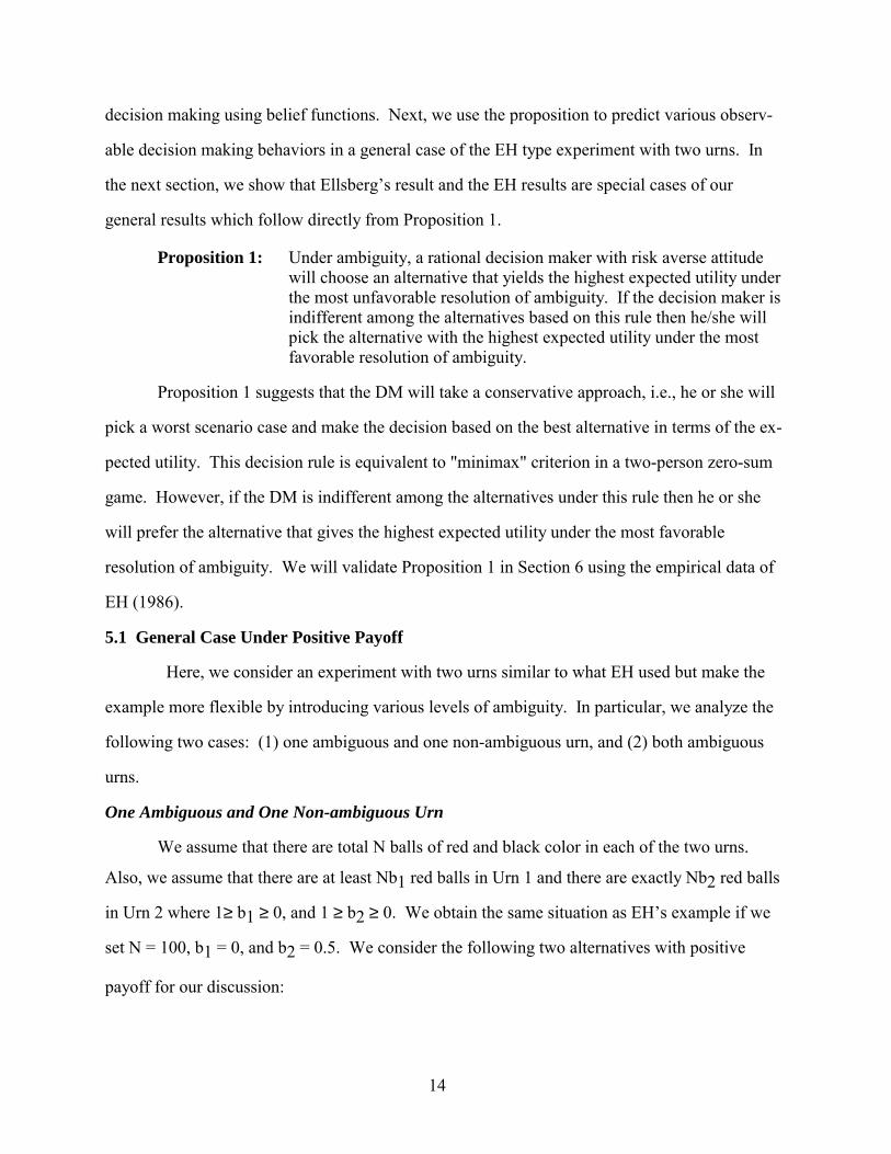
Proposition 1: Under ambiguity, a rational decision maker with risk averse attitude will choose an alternative that yields the highest expected utility under the most unfavorable resolution of ambiguity. If the decision maker is indifferent among the alternatives based on this rule then he/she will pick the alternative with the highest expected utility under the most favorable resolution of ambiguity.

Proposition 1 suggests that the DM will take a conservative approach, i.e., he or she will

pick a worst scenario case and make the decision based on the best alternative in terms of the ex-

pected utility. This decision rule is equivalent to "minimax" criterion in a two-person zero-sum

game. However, if the DM is indifferent among the alternatives under this rule then he or she

will prefer the alternative that gives the highest expected utility under the most favorable

resolution of ambiguity. We will validate Proposition 1 in Section 6 using the empirical data of

EH (1986).

5.1 General Case Under Positive Payoff

Here, we consider an experiment with two urns similar to what EH used but make the

example more flexible by introducing various levels of ambiguity. In particular, we analyze the

following two cases: (1) one ambiguous and one non-ambiguous urn, and (2) both ambiguous

urns.

One Ambiguous and One Non-ambiguous Urn

We assume that there are total N balls of red and black color in each of the two urns.

Also, we assume that there are at least Nb1 red balls in Urn 1 and there are exactly Nb2 red balls

in Urn 2 where 1≥ b1 ≥ 0, and 1 ≥ b2 ≥ 0. We obtain the same situation as EH�s example if we

set N = 100, b1 = 0, and b2 = 0.5. We consider the following two alternatives with positive

payoff for our discussion:

15

Win $X if you pick a red ball from Urn 1 and win $0 if you pick a black ball (ambiguous case).

Win $X if you pick a red ball from Urn 2 and win $0 if you pick a black ball (non-am-biguous).

The m-value and the belief that a red ball is picked from Urn 1 is b1 by construct since

we know that we have at least Nb1 red balls out of N total. When the red ball is picked the

player wins $X. Therefore, the belief that the DM wins if he/she picks a red ball from Urn 1 is

also b1. Moreover, we know in the case of Urn 1 that there could be a possibility that all the

balls are red. In that situation the maximum belief that could be assigned to picking a red ball

from Urn 1 is 1.0 which is the plausibility value. The m-value and the belief that a black ball is

picked from Urn 1 is zero. Similar arguments can be presented for Urn 2. Thus, m-values,

beliefs, and plausibilities for the two alternatives are given below:

Urn 1: m(R1) = b1, m(B1) = 0, i.e., Bel(R1) = b1, Bel(B1) = 0,

Pl(R1) = 1, Pl(B1) = 1�b1,

Ambiguity in R1 = 1�b1, and Ambiguity in B1 = 1�b1. (1)

Urn 2: m(R2) = b2, m(B2) = 1�b2, i.e., Bel(R2) = b2, Bel(B2) = 1�b2,

Pl(R2) = b2, Pl(B2) = 1�b2,

Ambiguity in R2 = 0, and Ambiguity in B2 = 0. (2)

According to Strat (1994), the reassigned m-values for Urn 1 with ρ being the probability

of resolving ambiguity as favorably as possible are given by:

m(R1) = b1 + (1�b1).ρ, m(B1) = (1�b1).(1�ρ). (3)

The expected utility in the case of Urn 1 is:

E(U1) = m(R1).U($X) + m(B1).U($0),

= [b1 + (1�b1).ρ].U($X) + [(1�b1).(1�ρ)].U($0), (4)

For the most unfavorable resolution of ambiguity (ρ = 0), we have:

16

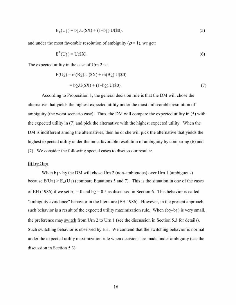
E*(U1) = b1.U($X) + (1�b1).U($0). (5)

and under the most favorable resolution of ambiguity (ρ = 1), we get:

E*(U1) = U($X). (6)

The expected utility in the case of Urn 2 is:

E(U2) = m(R2).U($X) + m(B2).U($0)

= b2.U($X) + (1�b2).U($0). (7)

According to Proposition 1, the general decision rule is that the DM will chose the

alternative that yields the highest expected utility under the most unfavorable resolution of

ambiguity (the worst scenario case). Thus, the DM will compare the expected utility in (5) with

the expected utility in (7) and pick the alternative with the highest expected utility. When the

DM is indifferent among the alternatives, then he or she will pick the alternative that yields the

highest expected utility under the most favorable resolution of ambiguity by comparing (6) and

(7). We consider the following special cases to discuss our results:

(i) b1< b2:

When b1< b2 the DM will chose Urn 2 (non-ambiguous) over Urn 1 (ambiguous)

because E(U2) > E*(U1) (compare Equations 5 and 7). This is the situation in one of the cases

of EH (1986) if we set b1 = 0 and b2 = 0.5 as discussed in Section 6. This behavior is called

"ambiguity avoidance" behavior in the literature (EH 1986). However, in the present approach,

such behavior is a result of the expected utility maximization rule. When (b2�b1) is very small,

the preference may switch from Urn 2 to Urn 1 (see the discussion in Section 5.3 for details).

Such switching behavior is observed by EH. We contend that the switching behavior is normal

under the expected utility maximization rule when decisions are made under ambiguity (see the

discussion in Section 5.3).

17

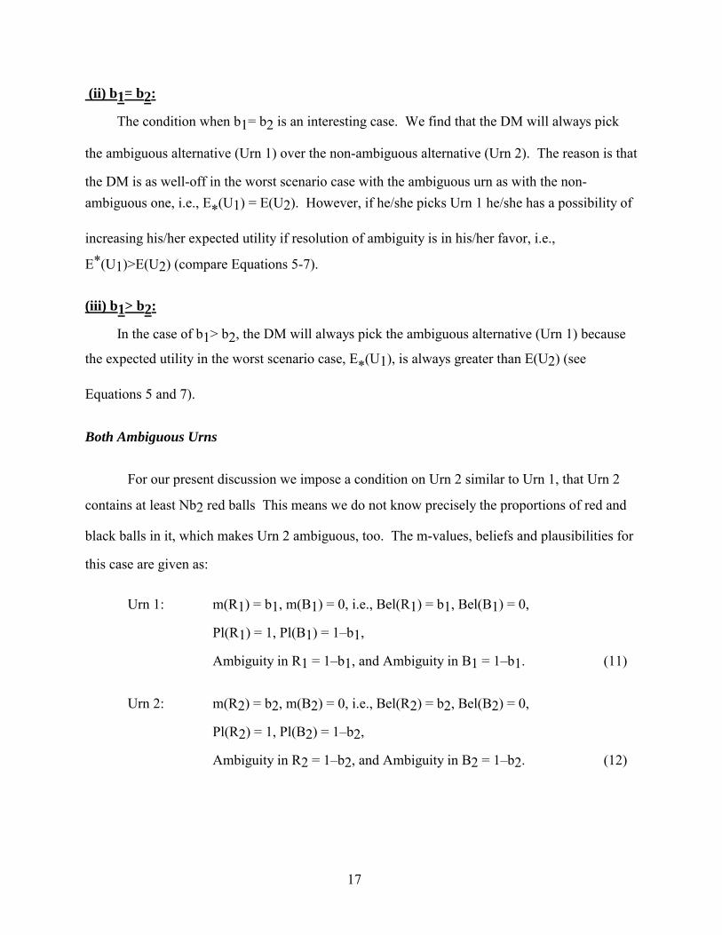
(ii) b1= b2:

The condition when b1= b2 is an interesting case. We find that the DM will always pick

the ambiguous alternative (Urn 1) over the non-ambiguous alternative (Urn 2). The reason is that

the DM is as well-off in the worst scenario case with the ambiguous urn as with the non-ambiguous one, i.e., E*(U1) = E(U2). However, if he/she picks Urn 1 he/she has a possibility of

increasing his/her expected utility if resolution of ambiguity is in his/her favor, i.e.,

E*(U1)>E(U2) (compare Equations 5-7).

(iii) b1> b2:

In the case of b1> b2, the DM will always pick the ambiguous alternative (Urn 1) because

the expected utility in the worst scenario case, E*(U1), is always greater than E(U2) (see

Equations 5 and 7).

Both Ambiguous Urns

For our present discussion we impose a condition on Urn 2 similar to Urn 1, that Urn 2

contains at least Nb2 red balls This means we do not know precisely the proportions of red and

black balls in it, which makes Urn 2 ambiguous, too. The m-values, beliefs and plausibilities for

this case are given as:

Urn 1: m(R1) = b1, m(B1) = 0, i.e., Bel(R1) = b1, Bel(B1) = 0,

Pl(R1) = 1, Pl(B1) = 1�b1,

Ambiguity in R1 = 1�b1, and Ambiguity in B1 = 1�b1. (11)

Urn 2: m(R2) = b2, m(B2) = 0, i.e., Bel(R2) = b2, Bel(B2) = 0,

Pl(R2) = 1, Pl(B2) = 1�b2,

Ambiguity in R2 = 1�b2, and Ambiguity in B2 = 1�b2. (12)

18

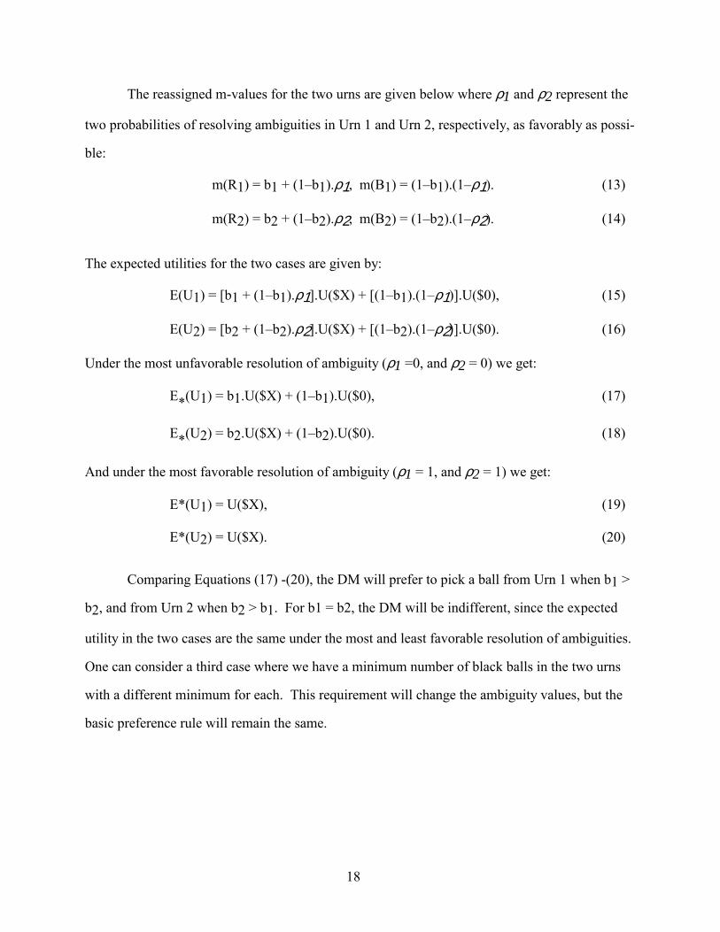
The reassigned m-values for the two urns are given below where ρ1 and ρ2 represent the

two probabilities of resolving ambiguities in Urn 1 and Urn 2, respectively, as favorably as possi-

ble:

m(R1) = b1 + (1�b1).ρ1, m(B1) = (1�b1).(1�ρ1). (13)

m(R2) = b2 + (1�b2).ρ2, m(B2) = (1�b2).(1�ρ2). (14)

The expected utilities for the two cases are given by:

E(U1) = [b1 + (1�b1).ρ1].U($X) + [(1�b1).(1�ρ1)].U($0), (15)

E(U2) = [b2 + (1�b2).ρ2].U($X) + [(1�b2).(1�ρ2)].U($0). (16)

Under the most unfavorable resolution of ambiguity (ρ1 =0, and ρ2 = 0) we get:

E*(U1) = b1.U($X) + (1�b1).U($0), (17)

E*(U2) = b2.U($X) + (1�b2).U($0). (18)

And under the most favorable resolution of ambiguity (ρ1 = 1, and ρ2 = 1) we get:

E*(U1) = U($X), (19)

E*(U2) = U($X). (20)

Comparing Equations (17) -(20), the DM will prefer to pick a ball from Urn 1 when b1 >

b2, and from Urn 2 when b2 > b1. For b1 = b2, the DM will be indifferent, since the expected

utility in the two cases are the same under the most and least favorable resolution of ambiguities.

One can consider a third case where we have a minimum number of black balls in the two urns

with a different minimum for each. This requirement will change the ambiguity values, but the

basic preference rule will remain the same.

19

5.2 General Case Under Negative Payoff

Let us consider again the example used earlier of two urns but with a negative payoff for

the two special cases: (1) one ambiguous and one non-ambiguous urn, and (2) both ambiguous

urns.

One Ambiguous and One Non-ambiguous Urn

The two alternatives for this case are:

Lose $X if you pick a red ball from Urn 1 and lose $0 if you pick a black ball (ambiguous case).

Lose $X if you pick a red ball from Urn 2 and lose $0 if you pick a black ball (non-am-biguous case).

Since there is no change in the information about the urns used earlier in Section 5.1 for a similar

case, we have the same values for m-values, beliefs, and plausibilities as given in (1) and (2):

According to Strat (1994), the reassigned m-values for Urn 1 with ρ being the probability

of resolving ambiguity as favorably as possible are given by :

m(R1) = b1 + (1�b1).(1�ρ), m(B1) = (1�b1).ρ.

Note the change in the allocation of ambiguity from (3) for a positive payoff to the m-values

given above for a negative payoff.

For the present situation, the expected utility in the case of Urn 1 is:

E(U1) = m(R1).U(�$X) + m(B1).U($0),

= [b1 + (1�b1).(1�ρ)].U(�$X) + [(1�b1)ρ].U($0).

For the most unfavorable resolution of ambiguity (ρ = 0), we have:

E*(U1) = U(�$X). (21)

and under the most favorable resolution of ambiguity (ρ = 1), we have

E*(U1) = b1.U(�$X) + (1�b1)U($0). (22)

The expected utility in the case of Urn 2 is:

E(U2) = m(R2).U(�$X) + m(B2).U($0)

20

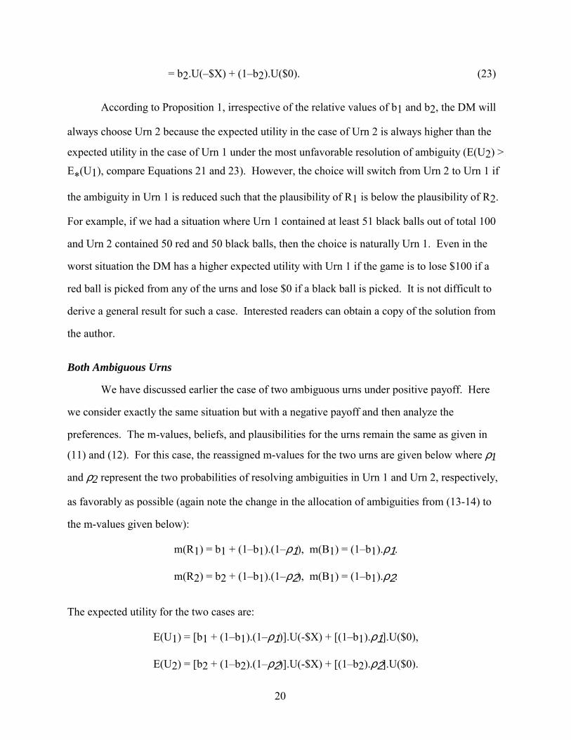
= b2.U(�$X) + (1�b2).U($0). (23)

According to Proposition 1, irrespective of the relative values of b1 and b2, the DM will

always choose Urn 2 because the expected utility in the case of Urn 2 is always higher than the

expected utility in the case of Urn 1 under the most unfavorable resolution of ambiguity (E(U2) >

E*(U1), compare Equations 21 and 23). However, the choice will switch from Urn 2 to Urn 1 if

the ambiguity in Urn 1 is reduced such that the plausibility of R1 is below the plausibility of R2.

For example, if we had a situation where Urn 1 contained at least 51 black balls out of total 100

and Urn 2 contained 50 red and 50 black balls, then the choice is naturally Urn 1. Even in the

worst situation the DM has a higher expected utility with Urn 1 if the game is to lose $100 if a

red ball is picked from any of the urns and lose $0 if a black ball is picked. It is not difficult to

derive a general result for such a case. Interested readers can obtain a copy of the solution from

the author.

Both Ambiguous Urns

We have discussed earlier the case of two ambiguous urns under positive payoff. Here

we consider exactly the same situation but with a negative payoff and then analyze the

preferences. The m-values, beliefs, and plausibilities for the urns remain the same as given in

(11) and (12). For this case, the reassigned m-values for the two urns are given below where ρ1

and ρ2 represent the two probabilities of resolving ambiguities in Urn 1 and Urn 2, respectively,

as favorably as possible (again note the change in the allocation of ambiguities from (13-14) to

the m-values given below):

m(R1) = b1 + (1�b1).(1�ρ1), m(B1) = (1�b1).ρ1.

m(R2) = b2 + (1�b1).(1�ρ2), m(B1) = (1�b1).ρ2.

The expected utility for the two cases are:

E(U1) = [b1 + (1�b1).(1�ρ1)].U(-$X) + [(1�b1).ρ1].U($0),

E(U2) = [b2 + (1�b2).(1�ρ2)].U(-$X) + [(1�b2).ρ2].U($0).

21

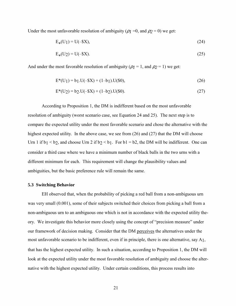
Under the most unfavorable resolution of ambiguity (ρ1 =0, and ρ2 = 0) we get:

E*(U1) = U(�$X), (24)

E*(U2) = U(�$X). (25)

And under the most favorable resolution of ambiguity (ρ1 = 1, and ρ2 = 1) we get:

E*(U1) = b1.U(�$X) + (1�b1).U($0), (26)

E*(U2) = b2.U(�$X) + (1�b2).U($0). (27)

According to Proposition 1, the DM is indifferent based on the most unfavorable

resolution of ambiguity (worst scenario case, see Equation 24 and 25). The next step is to

compare the expected utility under the most favorable scenario and chose the alternative with the

highest expected utility. In the above case, we see from (26) and (27) that the DM will choose

Urn 1 if b1 < b2, and choose Urn 2 if b2 < b1. For b1 = b2, the DM will be indifferent. One can

consider a third case where we have a minimum number of black balls in the two urns with a

different minimum for each. This requirement will change the plausibility values and

ambiguities, but the basic preference rule will remain the same.

5.3 Switching Behavior

EH observed that, when the probability of picking a red ball from a non-ambiguous urn

was very small (0.001), some of their subjects switched their choices from picking a ball from a

non-ambiguous urn to an ambiguous one which is not in accordance with the expected utility the-

ory. We investigate this behavior more closely using the concept of �precision measure� under

our framework of decision making. Consider that the DM perceives the alternatives under the

most unfavorable scenario to be indifferent, even if in principle, there is one alternative, say A1,

that has the highest expected utility. In such a situation, according to Proposition 1, the DM will

look at the expected utility under the most favorable resolution of ambiguity and choose the alter-

native with the highest expected utility. Under certain conditions, this process results into

22

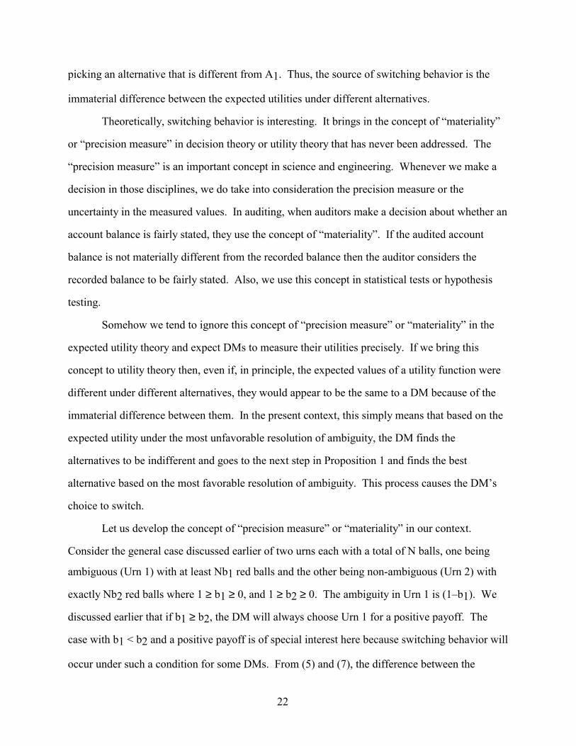
picking an alternative that is different from A1. Thus, the source of switching behavior is the

immaterial difference between the expected utilities under different alternatives.

Theoretically, switching behavior is interesting. It brings in the concept of �materiality�

or �precision measure� in decision theory or utility theory that has never been addressed. The

�precision measure� is an important concept in science and engineering. Whenever we make a

decision in those disciplines, we do take into consideration the precision measure or the

uncertainty in the measured values. In auditing, when auditors make a decision about whether an

account balance is fairly stated, they use the concept of �materiality�. If the audited account

balance is not materially different from the recorded balance then the auditor considers the

recorded balance to be fairly stated. Also, we use this concept in statistical tests or hypothesis

testing.

Somehow we tend to ignore this concept of �precision measure� or �materiality� in the

expected utility theory and expect DMs to measure their utilities precisely. If we bring this

concept to utility theory then, even if, in principle, the expected values of a utility function were

different under different alternatives, they would appear to be the same to a DM because of the

immaterial difference between them. In the present context, this simply means that based on the

expected utility under the most unfavorable resolution of ambiguity, the DM finds the

alternatives to be indifferent and goes to the next step in Proposition 1 and finds the best

alternative based on the most favorable resolution of ambiguity. This process causes the DM�s

choice to switch.

Let us develop the concept of �precision measure� or �materiality� in our context.

Consider the general case discussed earlier of two urns each with a total of N balls, one being

ambiguous (Urn 1) with at least Nb1 red balls and the other being non-ambiguous (Urn 2) with

exactly Nb2 red balls where 1 ≥ b1 ≥ 0, and 1 ≥ b2 ≥ 0. The ambiguity in Urn 1 is (1�b1). We

discussed earlier that if b1 ≥ b2, the DM will always choose Urn 1 for a positive payoff. The

case with b1 < b2 and a positive payoff is of special interest here because switching behavior will

occur under such a condition for some DMs. From (5) and (7), the difference between the

23

expected utility for Urn 2 and the expected utility for Urn 1 under the most unfavorable

resolution of ambiguity is given by: ∆E*(U2-1) = E(U2) � E*(U1),

= b2.U($X) + (1�b2).U($0) � b1.U($X) � (1�b1).U($0),

= (b2 � b1).[U($X) � U($0)] (28)

If the above difference is perceived to be insignificant or not �material� by the DM then he or she

feels indifferent about the two alternatives. But how do we measure whether the difference is in-

significant? Since we do not know the absolute values of the utility function at different wealth

levels, it is better that we define the difference in (28) to be material on the basis of the relative

value of the utility function. Thus, assume αc to be the critical value such that if the difference in

the expected utilities for the two alternatives is less than or equal to αc times the relative value of

the utility function then the DM is indifferent about the two alternatives, i.e., the difference is im-

material. In other words, for

∆E*(U2-1)/[U($X) � U($0)] = (b2 - b1) ≤ αc, (29)

the switching behavior will occur since the difference is not �material�. But if the above ratio is

greater than αc, then the difference is material, and the DM is able to distinguish between the

alternatives and hence there will be no switching.

One would like to know answers to such questions as: (1) What is the value of αc? (2)

What factors does it depend on? Well, we do not know the answers. To answer these questions

we need to perform empirical tests. However, we can make some speculations. For example, a

value of 0.01 for αc would suggest that the DM is not able to distinguish between alternatives

when the difference is 1 percent or less of the relative utility value. In response to the second

question, we can argue that the initial wealth level and the risk attitude of the DM will influence

the magnitude of αc. For a wealthy individual, the value of αc will be larger than for a person

with not as much wealth. Also, for a risk averse individual the value will be smaller than for a

person with risk seeking attitude. According to (29), the switching behavior will occur whenever

24

the difference (b2-b1) is less than or equal to the critical value αc (see Section 6 for further

discussion).

6. VALIDATION OF PROPOSITION 1 USING EINHORN AND HOGARTH DATA

In this section, we validate Proposition 1 by using the data of EH. As discussed in

Section 2.1, Ellsberg�s experiment was conducted with a positive payoff using two urns. EH

repeated Ellsberg�s experiment but for four different situations. In two situations, they used

exactly the same set of urns as used by Ellsberg but considered both a positive and a negative

payoff. In the other two situations, they used a different set of urns to make the probability of

picking a winning or losing ball from the unambiguous urn to be 0.001. We will discuss these

four cases below.

Case 1: Positive Payoff with probability 0.5

The first experiment of EH deals with a positive payoff and two urns. Urn 1 contains 100

red and black balls with unknown proportions. Urn 2 contains 50 red and 50 black balls. The

subjects are offered $100 if they pick a specific color ball (red or black) from one of the urns but

get $0 if they pick a wrong ball. The question they asked the participants is which urn would

they prefer to pick from?

This experiment is equivalent to our general case with a positive payoff (Section 5.1)

where X =100, N = 100, b1 = 0, and b2 = 0.5. However, for simplicity of presentation, we

assume that the participants will win $100 if they pick a red ball from either urn to be able to use

directly the results derived in (5-7). The treatment will be similar if the condition was based on

picking a black ball. Thus, using (5-7) we obtain the following expected values of utility for this

case. The expected utility in the case of Urn 1 for the most unfavorable resolution of ambiguity

is:

E*(U1) = U($0),

and under the most favorable resolution of ambiguity is:

25

E*(U1) = U($100).

The expected utility in the case of Urn 2 is:

E(U2) = 0.5U($100) + 0.5U($0).

According to Proposition 1, and knowing the fact that E(U2) > E*(U1) from the above

values, the DM will prefer to pick a red ball from Urn 2. EH (1986, see Table 1, p. S237, first

row) data support this result. Forty-seven percent of the subjects picked non-ambiguous urn (Urn

2), 19 percent ambiguous urn (Urn 1), and 34 percent were indifferent.

Case 2: Negative payoff with probability 0.5

This case uses the same set of urns as used in Case 1, but the payoff is negative. The par-

ticipants in the game are told that they will lose $100 if they pick a specified color ball and lose

$0 if they pick a wrong ball. Let us assume again, for simplicity of discussion, that the

participants are told that they will lose $100 if they pick a red ball but lose nothing if they pick a

black ball. This is a special case of our general case discussed in Section 5.2 with X = 100, N =

100, b1 = 0, and b2 = 0.5. Thus using (21-22), the expected utility in the case of Urn 1 for the

most unfavorable resolution of ambiguity is:

E*(U1) = U(-$100),

and under the most favorable resolution of ambiguity is

E*(U1) = U($0).

From (23), the expected utility in the case of Urn 2 is

E(U2) = 0.5U(-$100) + 0.5U($0).

Again according to Proposition 1, and knowing the fact that E(U2)>E*(U1) from the

above values, the DM will prefer to pick a red ball from Urn 2. The EH (1986, see Table 1, row

3) data support our result. Thirty percent chose Urn 2 (non-ambiguous), only 14 percent chose

Urn 1 (ambiguous), and 56 percent were indifferent.

26

Case 3: Positive payoff with probability 0.001

In this experiment, EH asked the participants to imagine two urns with 1,000 balls. These

balls are numbered. The participants are told that they will be paid $1,000 if they pick the ball

with number 687 from one of the urns, otherwise, they get $0. Along with it, they are told that

the balls in Urn 1 may all or none be marked 687. The balls in Urn 2 are sequentially marked

from 1 to 1,000. The question is which urn would they prefer to pick from?

This situation is equivalent to our general case discussed in Section 5.1 with X = 1,000, N

= 1,000, b1 = 0, and b2 = 0.001. Thus we can use (5-7) to determine the expected values of util-

ity for different alternatives. For Urn 1, the expected utility for the most unfavorable resolution

of ambiguity is:

E*(U1) = U($0),

and under the most favorable resolution of ambiguity it is:

E*(U1) = U($1,000).

The expected utility in the case of Urn 2 is:

E(U2) = 0.001.U($1,000) + 0.999.U($0).

Based on these expected values of utility it seems the DM should pick Urn 2 according to Proposition 1 because E(U2) > E*(U1). However, the difference between E(U2) and E*(U1) is

so small that some DMs would be indifferent about the two alternatives. In such a situation, ac-

cording to Proposition 1, the DM will make the decision based upon the most favorable resolu-

tion of ambiguity. In the present case, since E*(U1) > E(U2), the decision will be to pick a red

ball from Urn 1. This is the switching behavior described by EH. As discussed in Section 5.3,

the switching behavior will depend on the �measure of precision� or �materiality�, i.e., how

material the difference is between the expected utilities perceived by the DM. Also, as

mentioned in Section 5.3, this �precision measure� would depend on the initial wealth of the DM

and the risk attitude. Thus, not all DMs will switch their preferences at the same time. EH data

show this mixed pattern. Thirty-five percent of subjects picked Urn 1 (the ambiguous urn) in the

27

present case compared to nineteen percent in the previous case where probability of picking a

winning ball was 0.5 (rows 1 and 2 in Table 1 of EH, 1986). This result shows the switching

behavior. However, we see that still a significant percentage (43 percent) of DMs picked Urn 2

over Urn 1. The above result also makes intuitive sense. The DM has 999 chances out of 1,000

to win if he or she picks the ball from Urn 1 (ambiguous) and only one chance out 1,000 if he/she

picks from Urn 2 (non-ambiguous).

Case 4: Negative payoff with probability 0.001

This case is similar to Case 3 discussed above except the payoff is negative. The subjects

are told that they will lose $1,000 if they pick a ball marked 687. The question is which urn

would they choose? This situation is equivalent to our general case discussed in Section 5.2 with

X = 1,000, N = 1,000, b1 = 0, and b2 = 0.001. Thus we can use (21-23) directly to determine the

expected values of utility for different alternatives. For Urn 1, the expected utility for the most

unfavorable resolution of ambiguity is

E*(U1) = U(-$1,000),

and under the most favorable resolution of ambiguity, it is:

E*(U1) = U($0).

The expected utility in the case of Urn 2 is:

E(U2) = 0.001.U(-$1,000) + 0.999.U($0).

Based on these expected utilities it seems the DM should pick Urn 2 according to Proposition 1 because E(U2) > E*(U1). There will be no switching behavior in this case because

the two expected utilities (E*(U1) = U(-$1,000), and E(U2) = 0.001.U(-$1,000) + 0.999.U($0))

are very different. This case has very strong support from the EH data (1986, see Table 1, row

four). Seventy-five percent of the subjects chose Urn 2 (non-ambiguous), only 5 percent Urn 1

(ambiguous), and 20 percent were indifferent. This result again makes intuitive sense. The DM

has only one chance out of 1,000 to loose if he/she picks the ball from Urn 2 (non-ambiguous)

but has 999 chances out of 1,000 if he/she picks from Urn 1 (ambiguous).

28

7. SUMMARY AND CONCLUSION

In conclusion, we have shown how the belief-function framework can help us understand

the human decision making process under ambiguity. In particular, we have developed a

proposition for decision making under ambiguity using the expected utility theory under the

belief-function framework. This proposition is based on Strat�s approach (1990, 1994) of

resolving ambiguity in the problem. The proposition suggests that the DM will take a

conservative approach and use the most unfavorable resolution of ambiguity for making a

decision. If he or she is indifferent among the alternatives under this scenario, then he/she will

use the most favorable resolution of ambiguity and choose the alternative that has the maximum

expected utility. Using this proposition, we have explained the Ellsberg paradox. Also, we have

used the empirical data of EH (1986) to validate Proposition 1.

Using Proposition 1, we have predicted several observable behaviors of decision making

under ambiguity for the EH type experiment under four general situations: (1) positive payoff

with one ambiguous and one non-ambiguous urns, (2) positive payoff with both ambiguous urns,

(3) negative payoff with one ambiguous and one non-ambiguous urns, and (4) negative payoff

with both ambiguous urns. Also, we have discussed the general condition under which the

�switching� behavior will occur using the concept of �precision measure� in the expected utility

theory. In the context of Proposition 1, this concept simply means that the DM is indifferent

among the alternatives under the most unfavorable resolution of ambiguity, even though theoreti-

cally there is an alternative, say A1, that has the highest expected utility. Consequently, the DM

decides to pick an alternative based on the most favorable resolution of ambiguity which, under

certain conditions, may be different from A1.

29

FOOTNOTES

1. Strat�s approach is the only approach that explains Ellsberg�s paradox as shown in this article

2. A major portion of this section has been taken from Srivastava (1993).

3. In the case of n elements in the frame, we will have P(ai) ≥ 0, and P(ai)�i=1

n = 1, where ai repre-

sents the ith element of the frame.

4. For a frame of n elements, we will have, in general, m-values for each individual elements, each set of two elements, each set of three elements, and so on, to the m-value for the entire frame. All such m-values add to one, i.e., m(A)�

A⊆Θ = 1, where A represents all the proper sub-

sets of the frame Θ. The m-value for the empty set is zero.

5. The expected value interval, [E*(x), E*(x)], is given by (see, e.g., Strat 1990):

E*(x) = ΣAi⊆Θ

inf(Ai).m(Ai)

and

E*(x) = ΣAi⊆Θ

sup(Ai).m(Ai)

where inf(Ai) represents the smallest element in the set Ai ⊆ Θ and sup(Ai) represents the

largest element in the set Ai ⊆ Θ.

30

REFERENCES

Davis, R., Buchanan, B., and Shortliffe, E.H., �Production Rules as a Representation for a Knowledge-Based Consultation System,� Artificial Intelligence, 8, 1977, pp. 15-45.

Dubois, D., and Prade, H., �Necessity Measures and the Resolution Principle,� IEEE Transactions Systems, Man and Cybernetics, 17, 1987, pp. 474-478.

Dubois, D., and Prade, H., �Resolution Principles in Possibilistic Logic,� International Journal of Approximate Reasoning, 4(1), 1990, pp. 1-21.

Einhorn, H. J., and Hogarth, R. M., �Decision Making under Ambiguity,� The Journal of Business, 59(4), Pt. 2, October 1986, pp. S225-S250.

Einhorn, H. J., and Hogarth, R. M., �Ambiguity and Uncertainty in Probabilistic Inference,� Psychological Review, 92, 1985, pp. 433-461.

Ellsberg, D., �Risk, Ambiguity, and the Savage Axioms,� Quarterly Journal of Economics, 75, 1961, pp. 643-669.

Jaffray, J-Y., �Dynamic Decision Making with Belief Functions,� Advances in the Dempster-Shafer Theory of Evidence, edited by R.R. Yager, M. Fedrizzi, and J. Kacprzyk, John Wiley and Sons. New York, NY, 1994.

Jaffray, J-Y., �Utility Theory for Belief Functions,� Operations Research Letters, Vol. 8, 1989, pp. 107-12.

Kahneman, D., Slovic, P., and Tversky, A., Judgment under Uncertainty: Heuristics and Biases, Cambridge, England: Cambridge University Press, 1982.

Kahneman, D., and Tversky, A., �Prospect Theory: An Analysis of Decision Under Risk,� Econometrica, 47(2), 1979, pp. 263-291.

Nguyen H.T., and Walker, E.A., �On Decision Making Using Belief Functions,� Advances in the Dempster-Shafer Theory of Evidence, edited by R.R. Yager, M. Fedrizzi, and J. Kacprzyk, John Wiley and Sons. New York, NY, 1994.

Schoemaker, P. J. H., �The Expected Utility Model: Its Variants, Purposes, Evidence and Limitations,� Journal of Economic Literature XX, June 1982, pp. 529-563.

Shafer, G., A Mathematical Theory of Evidence, Princeton, N.J., Princeton University Press, 1976.

Shafer, G., and Srivastava, R.P. , �The Bayesian and Belief-Function Formalisms: A General Perspective for Auditing,� Auditing: A Journal of Practice and Theory, Supplement, 1990, pp. 110-148.

Smets, P., �The Combination of Evidence in the Transferable Belief Model,� IEEE Transactions on Pattern Analysis and Machine Intelligence 12, 5, May 1990a.

31

Smets, P., �Constructing the Pignistic Probability Function in a Context of Uncertainty,� Uncertainty in Artificial Intelligence 5, ed. by M. Henrion, R. D. Shachter, L. N. Kanal, and J. F. Lemmer, Elsevier Science Publishers B.V., North-Holland, 1990b.

Srivastava, R.P., �A Comparison of Decision Making Approaches Under Belief Functions,� Working Paper, School of Business, The University of Kansas, 1995.

Srivastava, R.P., �Belief Functions and Audit Decisions,� Auditors Report, 17(1), Fall 1993, pp. 8-12.

Srivastava, R.P., and Shafer, G., �Belief-Function Formulas for Audit Risk,� The Accounting Review, April 1992, pp. 249-83.

Strat, T.M., �Decision Analysis Using Belief Functions,� International Journal of Approximate Reasoning, vol. 4(5), 1990, p. 6.

Strat, T.M., �Decision Analysis Using Belief Functions,� Advances in the Dempster-Shafer Theory of Evidence, edited by R.R. Yager, M. Fedrizzi, and J. Kacprzyk, John Wiley and Sons. New York, NY, 1994.

Tversky, A, and Kahneman, D., �Rational Choice and the Framing of Decisions,� The Journal of Business, 59(4), Pt. 2, October 1986, pp. S251-78.

Wong, S.K.M., and Wang, Z.W., �Qualitative Measures of Ambiguity,� Proceedings of The Ninth Conference on Uncertainty in Artificial Intelligence, edited by Davis Hackerman and Abe Mamdani. Morgan Kaufmann, San Mateo, California, 1993, pp. 443-450.

Yager, R.R., �Decision making Under Dempster-Shafer Uncertainties,� Technical Report MII-915, Iona College, New Rochelle, NY, 1990.

Zadeh, L. A., �Fuzzy Sets,� Information Control, 8, 1965, pp. 338-53.