Embed Size (px)
Citation preview
Decision guide environment for design space exploration
Benoıt MiramondLaboratoire ETIS - UMR CNRS 8051
6, avenue du Ponceau BP 44F 95014 Cergy-Pontoise Cedex, France
Jean-Marc DelosmeLaboratoire LaMI UMR 8042 CNRS
Universite d’Evry Val d’Essonne523 Place des Terrasses 91000 Evry
Abstract
In current embedded system design practice, only fewarchitectural solutions and mappings of the functionalitiesof a system on the architecture’s components are exam-ined. This paper presents an optimization-based methodand the associated tool developed to help designers takearchitectural decisions. The principle of this approach isto efficiently explore the design space and to dynamicallyprovide the user with the capabilities to visualize the evo-lution of selected criteria. The first objective is solved bydeveloping an enhanced version of the adaptive simulatedannealing algorithm. Since the method is iterative, multi-ple solutions may be examined and the tool lets the userstop exploration at any time, tune parameters and selectsolutions.Moreover we present an approach for systems whose func-tionalities are specified by means of multiple models ofcomputation, in order to handle descriptions of digital sig-nal applications at several levels of detail.The tool has been applied to a motion detection applica-tion in order to determine architectural parameters.
1 Introduction
The steady increase of integrated circuit densities dur-ing the last three decades has been the driving force en-abling ever more sophisticated consumer products witha wealth of functionalities to reach the market. Theseproducts are most often embedded systems that becomeincreasingly more difficult to design. The complexityof both the hardware and the software in these systemsmakes them so hard to debug that delivering the productson time is a real challenge. The decisions about system ar-chitecture, the use of dedicated components (FPGAs) andthe selection of processors to be used as programmablecomponents impact design complexity and hence designtime and design cost. This process of defining the sys-tem architecture and of mapping its functionalities ontoits components determines for which functionalities soft-ware will have to be developed and for which ones hard-ware must be designed.
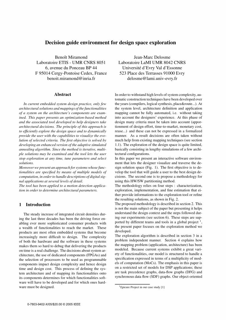
In order to withstand high levels of system complexity, au-tomatic construction techniques have been developed overthe years (compilers, logical synthesis, place&route...). Atthe system level, architecture definition and applicationmapping cannot be fully automated, i.e. without takinginto account the designers’ experience. At this phase ofdesign many criteria must be taken into account (appor-tionment of design effort, time-to-market, monetary cost,reuse...) and these can not be expressed in a formalizedmanner. As a result decisions are often taken withoutmuch help from existing mapping techniques (see section1.1). The exploration of the design space is quite limited,basically consisting in lengthy simulations of a few archi-tectural configurations.In this paper we present an interactive software environ-ment that lets the designer visualize and traverse the de-sign solution space (Fig. 1). The first objective is to de-velop the tool that will guide a user to the best design de-cisions. The second one is to propose a methodology forusing this HW/SW partitioning method.The methodology relies on four steps : characterization,exploration, implementation, and fine estimation that ei-ther provide informations to the exploration tool or refinethe resulting solutions, as shown in Fig. 2.The proposed methodology is described in section 2. Thisis not the main subject of the paper but presenting it helpsunderstand the design context and the steps followed dur-ing our experiments (see section 6). These steps are sup-ported by different teams and tools in a global project 1,the present paper focuses on the exploration method wedeveloped.The exploration algorithm is described in section 3 in aproblem independent manner. Section 4 explains howthe mapping problem (application, architecture) has beenmodeled. Because current systems exhibit a great vari-ety of functionalities, our model is structured to handle aspecification expressed in terms of a multiplicity of mod-els of computation (MoCs). The emphasis in this paper ison a restricted set of models for DSP applications; theseare task precedence graphs, data-flow graphs (DFG) andsynchronous data flow (SDF) graphs. Our object-oriented
1Epicure Project in our case study [1]
0-7803-9402-X/05/$20.00 © 2005 IEEE
environment facilitates the development of modules asso-ciated to each new MoC that we integrate in our tool. Theway of exploring the solution space for multi-model spec-ifications is presented in section 5. Experiments and re-
Figure 1. Principle of the 4OM tool.
sults obtained with the 4OM tool are presented in section6. Finally, perspectives are given in Section 7.
1.1 Related WorkArchitecture selection consists in two main types of de-
cision : allocation and mapping. Allocation is the defini-tion of architecture in terms of number and class of pro-cessors and hardware acceleration units. Mapping is thepartitioning of functional primitives on this selected re-sources.Much research has been done on automatic partition-ing. Among the first existing tools, COSYMA[8] andLYCOS[7] find optimal solutions when partitioning ap-plications on single processor architecture.In order to provide better performance, technology offersmultiprocessor SoCs that allow to exploit more efficientlycoarse grain parallelism. The SpecSyn tool proposedsince 1993 [6] supports multiprocessor architectures butassumes manual allocation. Moreover, when consider-ing the mapping selection process, SpecSyn proposes onlyone solution to the designer, and thus is not suited to ourexploration objective. More recent approaches treat thedesign space exploration problem for SoCs with multipleprocessors and HW accelerators, and consider both alloca-tion and mapping selection. These approaches use eitherexhaustive search [15], by iteratively adding resourceswhen constraints are violated, or optimization heuristics.In this last case, the optimization criterion can be a func-tion of chip area [11], or of the cost of the computing units[4]. These criteria give a very partial view of the alloca-tion consequences as discussed below, and a good opti-mization criterion would be very difficult to estimate [2][5].Moreover most of the algorithms used in current explo-ration tools depend on parameters (in the cost function or
in the algorithm itself) and need long tuning phases thatmake their practical use complicated.
1.2 ContributionsIn [13] we described in details the results obtained with
our exploration method on a motion detection application.In view of the existing codesign methodology and the cor-responding partitioning tools, our objectives in this paperand our contributions in the actual technological and re-search context are to propose a
• designer based exploration method where the objec-tive is to satisfy designer requirements. This is en-sured by an iterative optimization method (simulatedannealing), presented in section 3 and an interactivegraphical interface that we will describe in section 6.
• flexible exploration environment. For the algorith-mic part, the optimization method is based on anadaptive version of simulated annealing, and for thespecification part, our method aims at consideringheterogeneous applications. For this reason our inputspecification is assumed to be composed of multiplemodels of computation.
• global exploration methodology which provides thepractical utilization context of our tool. This method-ology was followed during our experiments.
2 Methodology
We follow a standard (part of) top-down design flow,including specification, design space exploration andhardware/software co-design steps. The paper focuses onthe HW/SW partitioning phase, but details about speci-fication (before partitioning) and performance estimation(after partitioning) give an overall understanding of theway we realized exploration with our tool in the experi-mental stages. The approach is built to exploit the relevantinformation at each abstraction level and then to minimizedesign effort.
2.1 CharacterizationThis phase which provides basic informations about
performances, area, memory, power consumption is a crit-ical point of most partitioning approaches since decisionstaken during the exploration step depend on the providedinformations. The practical case study used during exper-iments is part of the EPICURE project. In this context, thewell known target architecture (ARM9 processor + VirtexIC) allowed the use of associated design software (compil-ers), to perform simulations and then to extract a data basecontaining information about various implementations ofprimitives. In this dedicated context, multiple implemen-tations of a functionality where described on the HW unitwith different couples (execution time, number of config-urable logic blocks). Details about applications character-ization can be found in [13]. The need of relevant esti-
2
mates, and then of dedicated tools for architectural com-ponents is another motivation to limit the capacity of ourexploration method to fixed allocation design problems.
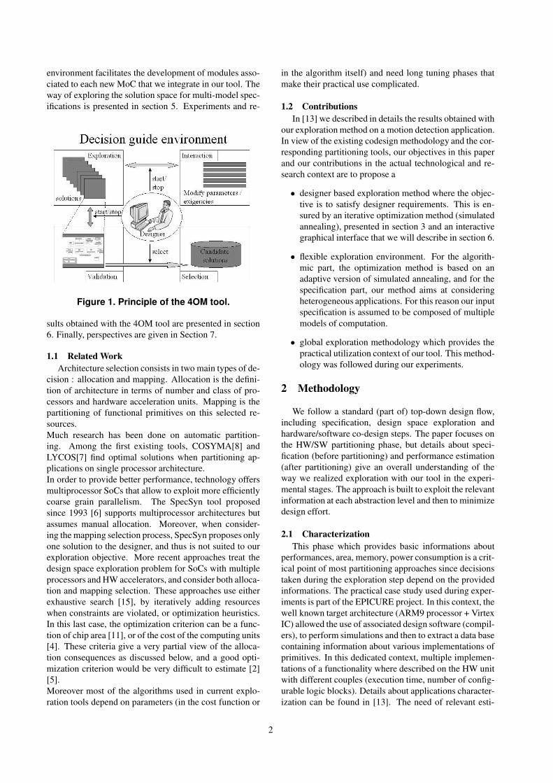
Figure 2. Design methodology.
2.2 Implementation modelThe solutions obtained when solving the partitioning
problem are abstract in that the same solution may beused with different implementation models. A classifi-cation of these models is proposed in [16]; the more thetask lengths depend on data values, the more dynamic (vs.static) decisions must be made, and the more the control(HW or SW) is complex. Models are—following thatorder—fully-static (FS), ordered-transaction (OT), self-timed (ST), quasi-static, static-assignment and fully dy-namic. The FS model applies when task durations are dataindependent or their largest values are close enough totheir average values to be used with little loss in through-put. Then, task starting times are determined at compiletime (by exploration) and control is simple. As the tasklength variances increase, the OT model becomes rele-vant; the ordering of the task executions and of the com-munications is determined at compile time but not thestarting times, which are determined at run time throughexplicit synchronization mechanisms (send and receive).Next, for higher variances, the ST model, for which onlythe ordering of the task executions is determined at com-pile time, becomes the most suitable.The partitioning algorithm determines task orderings aspart of the optimization process. Average performance iscomputed using average performance values for the func-tional objects obtained during the functionality character-ization step that precedes architecture definition (duringexploration). Variance and extreme values of performanceof the functional objects are used to determine candidateimplementation models (choice made at the level of the
outer loop of Fig. 2).
2.3 Performance estimationIn general the performances of complex systems de-
pend on the times at which their inputs are received andon the values of these inputs. Often there will be require-ments not only on average performance but also on theprobability of occurrence of poor (close to worst case) per-formance. To check that a solution found for the partition-ing problem will satisfy low probability of poor perfor-mance requirements a statistical simulation is used. Thisis a refined global performance estimation step whoseresults—success or failure and by how much—are fedback to the architecture definition (optimization) step.The “architecture definition” computations (optimizationinner loop) and the “performance estimation” computa-tions (simulations), see Fig. 2, are of similar complex-ity. The feedback “law” (adjustment of safety margins)requires particular attention: the number of iterations ofthe outer loop must be kept small to avoid spending morethan a few hours of computations on a workstation. In thecase the rigorous real-time context of our experiments, asingle global iteration of the methodology has been used.
3 Optimization method
3.1 Local search and simulated annealingIn order to efficiently2 explore design solution space
we use a local search method which proposes a completesolution to the optimization problem at each iteration.This first characteristic is important since the method pro-poses a set of solutions during its computation in contrastwith greedy approaches (such as list scheduling basedalgorithms) which build a single solution by means ofspecifically defined construction rules. For this reason, inour context local search seems to be the good candidate toperform an “exploration”. A local search algorithm startsfrom an initial solution, proposed or random, and modifiesit iteratively; these modifications are called “moves”.A solution is accepted only if its “cost” is found lower thanprevious values, the search process will end when no localmove decreases the cost further and the final solution is alocal optimum. In order to converge to a solution close to aglobal optimum, we use a simulated annealing algorithm.A solution that increases the cost is then accepted with aprobability that depends on a parameter: the temperature,denoted T (its inverse being denoted s). The way the tem-perature is controlled is called an annealing schedule; itgives the algorithm its convergence properties. A classi-cal annealing schedule keeps temperature constant duringsteps of the order of a hundred iterations and then lowersT according to a fixed multiplicative factor (∆ < 1):
T+ = ∆ · T.
With this schedule, it is hard to tune ∆ to attain a desiredquality of solution for a given problem instance and the
2hence not exhaustively
3
callMove
modelSelect
Get move set
Specification
DFG SDF
Performancedata offunctionalobjects
constraintsGet
variablesConstrained
Cost
handlingConstraints
Exploration
Simulated
Annealing
Estimation
Cost Performances
Optimisation
Estimation
Specification
ConcernPerformance
Datadependencies
Performancerequirements
AveragePerformanceEstimation
constraintsvariables to
constrained
Comparison of
PSfrag replacements
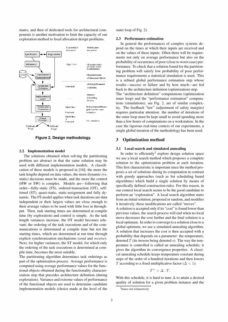
Figure 3. Software architecture of the explo-ration tool.
tradeoff between quality of solution and computation timeis poor.This motivated us to use an adaptive annealing schedule(section 3.2). We have developed an improved version ofLam’s adaptive SA algorithm [9] that provides solutionsof a desired quality—the tradeoff “quality vs. computa-tion time” being controlled by a single parameter—withvery good statistical stability (i.e. final cost has a smallvariance).
3.2 Adaptive simulated annealingTo perform a search that reaches a solution at most
a few percent away from the global optimum, we havepursued the work carried out by LAM, who presented in[9] both an adaptive cooling schedule and a scheme formove selection that speed up significantly the convergenceof simulated annealing. Adaptive SA employs a coolingschedule whose general form is independent of the opti-mization problem at hand. The problem’s cost function isviewed as the energy of a dynamical system whose statesare the problem’s solutions. The schedule is obtained bymaximizing the rate at which the temperature can be de-creased subject to the constraint that the system be main-tained in quasi-equilibrium. The adaptive nature of theschedule comes from the fact that it is expressed in termsof statistical quantities (mean µ(s), variance σ(s), corre-lation r(s)) of the system’s cost function :
sk+1 = sk + λ1 − r(sk)
σ(sk). (1)
where λ is the parameter whose value controls the trade-off between quality of solution and execution time (itrepresents the allowed distance to the quasi-equilibrium).Move generation affects the correlation between consecu-tive cost values and the adaptive schedule specifies how tocontrol move generation to maximize cooling speed while
satisfying the quasi-equilibrium condition. This version ofsimulated annealing has been used in VLSI circuit placeand route tools [17]. We have recently improved on theestimation procedure (for µ and σ) and also refined the se-lection of the moves. These modifications have been val-idated on several types of problems, including graph par-titioning and function minimization as explained in [12],but this is out of the scope of this paper.
3.3 Software architectureThe partitioning software environment is decomposed
into three independent modules: exploration, estimationand specification, see Fig. 3.The exploration module, the heart of the environment (atthe bottom of Fig. 3), implements the exploration and op-timization algorithms and includes a constraint manage-ment module. The current optimization algorithm is usedto optimize system performance but the ”cost” module canbe easily adapted to different criteria. This algorithmic en-gine is completely independent of the problem it solves:cost function and constraints are just data. Constraints areindependent of the cost function (in contrast e.g. with [18]where they are integrated in the cost function) and the al-gorithm is adaptive so that it does not need the user to setor tune parameters according to the problem. Constraintsare relaxed at the beginning of the exploration and hard-ened adaptively until they become strict, for the last itera-tions.The set of moves embodies decisions to modify architec-ture, assignment and scheduling. The moves are tailoredto each MoC and supplied by the specification module.They are devised so that any potentially interesting solu-tion may be reached. If not interrupted, the algorithm con-verges toward a solution close to a global optimum [12].
4 Problem modeling
4.1 ScenariosOur HW/SW partitioning methodology must be able to
handle a diversity of scenarios:- The system architecture is set because an existing SoCfrom the previous generation of the product is reused.Only the assignment and scheduling of the tasks on thecomponents have to be determined and just software willhave to be developed.- Some components of the architecture are known in ad-vance (such as a licensed IP3 core) and parts of the ap-plication are allocated on these components at the outset.Partitioning must be solved for the remaining parts of theapplication with some components imposed.- The product is new and an architecture that will achievethe desired performances has to be determined. A varietyof solutions must be proposed according to the constraintsand scenarios (e.g. investment in a particular IP license)contemplated by the project leader.Although our method has been applied to the three classes
3Intellectual Property
4
of problem, a great difficulty is the definition of good op-timization criteria when allocation is not fixed, as men-tioned above. Consequently, in the rest of the paper weconsider that allocation is fixed (first and second scenario).In our tool, the requirements of a given scenario are storedin configuration files and the exploration process may becontrolled by means of an interactive interface as dis-cussed in section 6.
Total Order Locally Partial OrderGlobally Total
���������������
���������������
���������������
���������������
�����������������������������������
���������������������
�����������������������������������
�����������������������������������
DRC
Proc
Com
A
G
F
H
0 3010 20
C
D
I JE
B
Element ClassProcessingabstract public abstract void schedule(Vs, Vd)
Class ASIC/ContextClass
ReconfigurableCircuit Class
Processor
ExecutionContext 1
ExecutionContext 2
CE BD
4
3
1
3
4
5 6
5
6
5
Reconfiguration(c)
(b)(a)
C
A
B
E
J
I
D
F
G
H
E
C D
A B
F G
H
I
J
PSfrag replacements
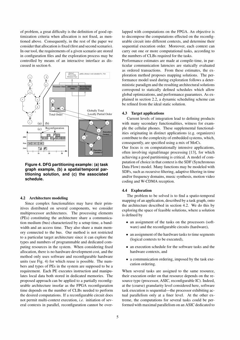
Figure 4. DFG partitioning example: (a) taskgraph example, (b) a spatial/temporal par-titioning solution, and (c) the associatedschedule.
4.2 Architecture modelingSince complex functionalities may have their prim-
itives distributed on several components, we considermultiprocessor architectures. The processing elements(PEs) constituting the architecture share a communica-tion medium (bus) characterized by a setup time, a band-width and an access time. They also share a main mem-ory connected to the bus. Our method is not restrictedto a particular target architecture since it can explore thetypes and numbers of programmable and dedicated com-puting resources in the system. When considering fixedallocation, there is no hardware development cost, and themethod only uses software and reconfigurable hardwareunits (see Fig. 4) for which reuse is possible. The num-bers and types of PEs in the system are supposed to be arequirement. Each PE executes instruction and manipu-lates local data both stored in dedicated memories. Theproposed approach can be applied to a partially reconfig-urable architecture insofar as the FPGA reconfigurationtime depends on the number of CLBs needed to performthe desired computations. If a reconfigurable circuit doesnot permit multi-context execution, i.e. initiation of sev-eral contexts in parallel, reconfiguration cannot be over-
lapped with computations on the FPGA. An objective isto decompose the computations effected on the reconfig-urable circuit into different contexts, and determine theirsequential execution order. Moreover, each context cancarry out one or more computational tasks, according tothe numbers of CLBs required for the tasks.Performance estimates are made at compile-time, in par-ticular communication latencies are statically evaluatedas ordered transactions. From these estimates, the ex-ploration method proposes mapping solutions. The per-formance model used during exploration follows a deter-ministic paradigm and the resulting architectural solutionscorrespond to statically defined schedules which allowglobal optimizations, and performance guarantees. As ex-plained in section 2.2, a dynamic scheduling scheme canbe refined from the ideal static solution.
4.3 Target applicationsCurrent levels of integration lead to defining products
with many secondary functionalities, witness for exam-ple the cellular phones. These supplemental functional-ities originating in distinct applications (e.g. organizers)contribute to the complexity of embedded systems, which,consequently, are specified using a mix of MoCs.Our focus is on computationally intensive applications,often involving signal/image processing [13], for whichachieving a good partitioning is critical. A model of com-putation of choice in that context is the SDF (SynchronousData Flow) model. Many functions may be modeled withSDFs, such as recursive filtering, adaptive filtering in timeand/or frequency domains, music synthesis, motion videocoding and W-CDMA reception.
4.4 ExplorationThe problem to be solved is to find a spatio-temporal
mapping of an application, described by a task graph, ontothe architecture described in section 4.2. We do this byexploring the space of feasible solutions, where a solutionis defined by
• an assignment of the tasks on the processors (soft-ware) and the reconfigurable circuits (hardware),
• an assignment of the hardware tasks to time segments(logical contexts to be executed),
• an execution schedule for the software tasks and thehardware contexts, and
• a communication ordering, imposed by the task exe-cution ordering.
When several tasks are assigned to the same resource,their execution order on that resource depends on the re-source type (processor, ASIC, reconfigurable IC). Indeed,at the (coarse) granularity level considered here, softwaretask execution is sequential—the processor exhibiting ac-tual parallelism only at a finer level. At the other ex-treme, the computations for several tasks could be per-formed with maximal parallelism on an ASIC dedicated to
5
PSfrag replacements PSfrag replacements
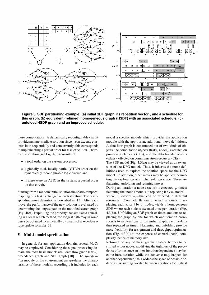
Figure 5. SDF partitioning example: (a) initial SDF graph, its repetition vector q and a schedule forthis graph, (b) equivalent (retimed) homogeneous graph (HSDF) with an associated schedule, (c)unfolded HSDF graph and an improved schedule.
these computations. A dynamically reconfigurable circuitprovides an intermediate solution since it can execute con-texts both sequentially and concurrently; this correspondsto implementing a partial order for task execution. There-fore, a solution (see Fig. 4(b)) consists of
• a total order on the system processor,
• a globally total, locally partial (GTLP) order on thedynamically reconfigurable logic circuit, and,
• if there were an ASIC in the system, a partial orderon that circuit.
Starting from a random initial solution the spatio-temporalmapping of a task is changed at each iteration. The corre-sponding move definition is described in [13]. After eachmove, the performance of the new solution is evaluated bydetermining the longest path in the modified search graph(Fig. 4(c)). Exploiting the property that simulated anneal-ing is a local search method, the longest path may in somecases be obtained incrementally by means of a Woodbury-type update formula [3].
5 Multi-model specification
In general, for any application domain, several MoCsmay be employed. Considering the signal processing do-main, the most basic models are : data flow graph (DFG),precedence graph and SDF graph [10]. The specifica-tion module of the environment encapsulates the charac-teristics of these models, accordingly it includes for each
model a specific module which provides the applicationmodule with the appropriate additional move definitions.A data flow graph is constructed out of two kinds of ob-jects, the computation objects (tasks, nodes), executed onprocessing elements (PEs), and the data transfer objects(edges), effected on communication resources (CEs).The SDF model (Fig. 4.3(a)) may be viewed as an exten-sion of the DFG model. Thus, it inherits the move def-initions used to explore the solution space for the DFGmodel. In addition, other moves may be applied, permit-ting the exploration of a richer solution space. These areflattening, unfolding and retiming moves.During an iteration a node i (actor) is executed qi times;flattening that node amounts to replacing it by ni nodes—where ni divides qi—that can be affected to differentresources. Complete flattening, which amounts to re-placing each actor i by qi nodes, yields a homogeneousSDF, where each node is executed once per iteration (Fig.4.3(b)). Unfolding an SDF graph m times amounts to re-placing the graph by one for which one iteration corre-sponds to m iterations of the initial graph; each node isthus repeated m times. Flattening and unfolding providemore flexibility for assignment and throughput optimiza-tion (Fig. 4.3(c)) at the expense of control (code) com-plexity, hence of memory size.Retiming of any of these graphs enables buffers to beshifted across nodes, modifying the tightness of the prece-dences (for instance an inter-iteration dependence may be-come intra-iteration while the converse may happen foranother dependence); this widens the space of possible or-derings. Assuming overlap between iterations for highest
6
FPGA Execution TRinitial+ Number Numbersize time TRdynamic of of
(CLBs) (ms) (ms) contexts tasks100 77.4 0.5 + 0.7 2.8 4.5200 41.6 1.0 + 6.1 8.3 13.1300 43.0 1.4 + 5.9 6 16.8400 22.4 1.9 + 11.8 9.2 15.4500 19.9 2.4 + 11.9 7.7 14.9600 23.9 3.0 + 12.2 7 18.3700 19.7 3.4 + 12.8 6.7 20.4800 18.4 3.4 + 12.7 6.4 18.2900 21.1 4.2 + 14.7 5.9 18.6
1000 20.0 4.2 + 14.4 5.9 16.01500 21.2 4.6 + 13.1 4.2 19.62000 25.8 10.0 + 12.2 3.5 19.13000 28.7 15.0 + 7.0 2.6 22.44000 29.2 19.1 + 4.3 2 20.95000 33.5 24.5 + 0 1 23.510000 35.9 27.3 + 0 1 24.2
Table 1. Average execution time and recon-figuration time (initial + dynamic), and av-erage number of contexts and of tasks asfunctions of FPGA size.
performance, the throughput is evaluated by constructingthe associated inter-processor communication (IPC) graphand calculating the maximum cycle mean4, whose inverseis the estimated throughput [16] (substituting performancemodule in Fig.3.
6 Experiments
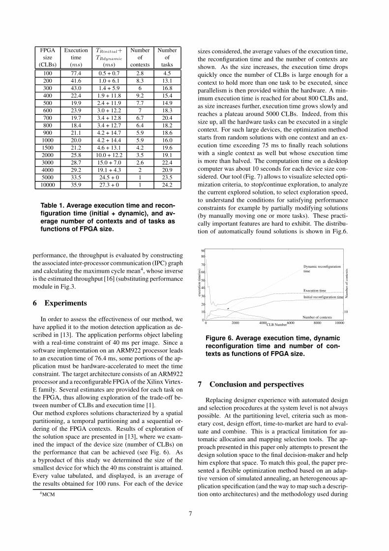
In order to assess the effectiveness of our method, wehave applied it to the motion detection application as de-scribed in [13]. The application performs object labelingwith a real-time constraint of 40 ms per image. Since asoftware implementation on an ARM922 processor leadsto an execution time of 76.4 ms, some portions of the ap-plication must be hardware-accelerated to meet the timeconstraint. The target architecture consists of an ARM922processor and a reconfigurable FPGA of the Xilinx Virtex-E family. Several estimates are provided for each task onthe FPGA, thus allowing exploration of the trade-off be-tween number of CLBs and execution time [1].Our method explores solutions characterized by a spatialpartitioning, a temporal partitioning and a sequential or-dering of the FPGA contexts. Results of exploration ofthe solution space are presented in [13], where we exam-ined the impact of the device size (number of CLBs) onthe performance that can be achieved (see Fig. 6). Asa byproduct of this study we determined the size of thesmallest device for which the 40 ms constraint is attained.Every value tabulated, and displayed, is an average ofthe results obtained for 100 runs. For each of the device
4MCM
sizes considered, the average values of the execution time,the reconfiguration time and the number of contexts areshown. As the size increases, the execution time dropsquickly once the number of CLBs is large enough for acontext to hold more than one task to be executed, sinceparallelism is then provided within the hardware. A min-imum execution time is reached for about 800 CLBs and,as size increases further, execution time grows slowly andreaches a plateau around 5000 CLBs. Indeed, from thissize up, all the hardware tasks can be executed in a singlecontext. For such large devices, the optimization methodstarts from random solutions with one context and an ex-ecution time exceeding 75 ms to finally reach solutionswith a single context as well but whose execution timeis more than halved. The computation time on a desktopcomputer was about 10 seconds for each device size con-sidered. Our tool (Fig. 7) allows to visualize selected opti-mization criteria, to stop/continue exploration, to analyzethe current explored solution, to select exploration speed,to understand the conditions for satisfying performanceconstraints for example by partially modifying solutions(by manually moving one or more tasks). These practi-cally important features are hard to exhibit. The distribu-tion of automatically found solutions is shown in Fig.6.
Initial reconfiguration time
Execution time
Number of contexts 10000 8000 6000 4000 2000 0 CLB Number
10
20
30
40
50
60
70
80
0
exec
utio
n tim
e(us
)
Num
ber o
f con
text
s
10
Dynamic reconfigurationtime
90
PSfrag replacements
Figure 6. Average execution time, dynamicreconfiguration time and number of con-texts as functions of FPGA size.
7 Conclusion and perspectives
Replacing designer experience with automated designand selection procedures at the system level is not alwayspossible. At the partitioning level, criteria such as mon-etary cost, design effort, time-to-market are hard to eval-uate and combine. This is a practical limitation for au-tomatic allocation and mapping selection tools. The ap-proach presented in this paper only attempts to present thedesign solution space to the final decision-maker and helphim explore that space. To match this goal, the paper pre-sented a flexible optimization method based on an adap-tive version of simulated annealing, an heterogeneous ap-plication specification (and the way to map such a descrip-tion onto architectures) and the methodology used during
7
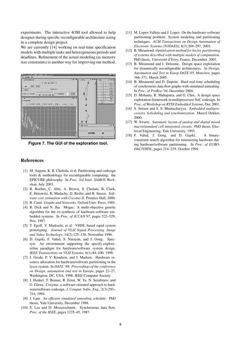
experiments. The interactive 4OM tool allowed to helpdesigner during specific reconfigurable architecture sizingin a complete design project.We are currently [14] working on real-time specificationmodels with multiple tasks and heterogeneous periods anddeadlines. Refinement of the actual modeling (as memorysize constraints) is another way for improving our method.
PSfrag replacements
Figure 7. The GUI of the exploration tool.
References
[1] M. Auguin, K. B. Chehida, et al. Partitioning and codesigntools & methodology for reconfigurable computing: theEPICURE philosophy. In Proc. 3rd Intnl. SAMOS Work-shop, July 2003.
[2] B. Boehm, C. Abts, A. Brown, S. Chulani, B. Clark,E. Horowitz, R. Madachy, D. Reifer, and B. Steece. Soft-ware cost estimation with Cocomo II. Prentice Hall, 2000.
[3] B. Carre. Graphs and Networks. Oxford Univ. Press, 1985.[4] R. Dick and N. Jha. Mogac: A multi-objective genetic
algorithm for the co-synthesis of hardware-software em-bedded systems. In Proc. of ICCAD’97, pages 522–529,Nov. 1997.
[5] T. Egolf, V. Madisetti, et al. VHDL based rapid systemprototyping. Journal of VLSI Signal Processing, Imageand Video Technology, 14(2):125–156, November 1996.
[6] D. Gajski, F. Vahid, S. Narayan, and J. Gong. Spec-syn: An environment supporting the specify-explore-refine paradigm for hardware/software system design.IEEE Transactions on VLSI Systems, 6(1):84–100, 1998.
[7] J. Grode, P. V. Knudsen, and J. Madsen. Hardware re-source allocation for hardware/software partitioning in thelycos system. In DATE ’98: Proceedings of the conferenceon Design, automation and test in Europe, pages 22–27,Washington, DC, USA, 1998. IEEE Computer Society.
[8] J. Henkel, T. Benner, R. Ernst, W. Ye, N. Serafimov, andG. Glawe. Cosyma: a software-oriented approach to hard-ware/software codesign. J. Comput. Softw. Eng., 2(3):293–314, 1994.
[9] J. Lam. An efficient simulated annealing schedule. PhDthesis, Yale University, December 1988.
[10] E. Lee and D. Messerschmitt. Synchronous data flow.Proc. of the IEEE, pages 1235–45, 1987.
[11] M. Lopez-Vallejo and J. Lopez. On the hardware-softwarepartitioning problem: System modeling and partitioningtechniques. ACM Transactions on Design Automation ofElectronic Systems (TODAES), 8(3):269–297, 2003.
[12] B. Miramond. Optimization method for hw/sw partitioningof systems described with multiple models of computation.PhD thesis, Universite d’Evry, France, December. 2003.
[13] B. Miramond and J. Delosme. Deisgn space explorationfor dynamically reconfigurable architectures. In Design,Automation and Test in Europ DATE’05, Munchen, pages366–371, March 2005.
[14] B. Miramond and D. Dupont. Hard real-time schedulingof synchronous data flow graphs with simulated annealing.In Proc. of ProRisc’04, December 2004.
[15] D. Mohanty, R. Mahapatra, and G. Choi. A design spaceexploration framework in multiprocessor SoC codesign. InProc. of Workshop on RTSS Embedded Systems, Dec 2001.
[16] S. Sriram and S. S. Bhattacharyya. Embedded multipro-cessors. Scheduling and synchronization. Marcel Dekker,2000.
[17] W. Swartz. Automatic layout of analog and digital mixedmacro/standard cell integrated circuits. PhD thesis, Elec-trical Engineering, Yale University, 1993.
[18] F. Vahid, J. Gong, and D. Gajski. A binary-constraint search algorithm for minimizing hardware dur-ing hardware/software partitioning. In Proc. of EURO-DAC/VHDL, pages 214–219, October 1994.
8