DECISION ANALYSIS: INTRODUCTION - Angelfire: … · 2005-09-12 · Métodos Cuantitativos M. En C. Eduardo Bustos Farias 2 Agenda Decision analysis in general Structuring decision

MétodosCuantitativos M. En C. Eduardo Bustos Farias 1

DECISION ANALYSIS:INTRODUCTION


AgendaDecision analysis in generalStructuring decision problemsDecision making under uncertainty -without probability informationDecision making under uncertainty -with probability informationValue of informationSummary


Making a DecisionWe all make decisions..everyday…Some of them are trivial and some are really importantSome decisions are simple and some are really complex

What makes a Decision Hard?UncertaintyTradeoffs..

Decision Analysis is a coherent procedure to decision making


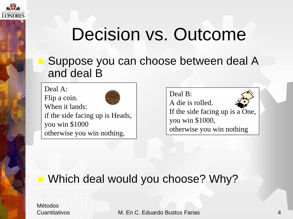
Decision vs. OutcomeSuppose you can choose between deal A and deal B

Which deal would you choose? Why?

Deal A:Flip a coin. When it lands:if the side facing up is Heads, you win $1000otherwise you win nothing.

Deal A:Flip a coin. When it lands:if the side facing up is Heads, you win $1000otherwise you win nothing.

Deal B: A die is rolled. If the side facing up is a One,you win $1000,otherwise you win nothing

Deal B: A die is rolled. If the side facing up is a One,you win $1000,otherwise you win nothing


Decision vs. OutcomeSuppose the coin is flipped and the die is rolled. The results are a Tails and a One.Do you still think you made a good decision?

If you were given another opportunity to choose between deal A and deal B before flipping the coin and rolling the die again, which would you choose?


Decision vs. OutcomeUnder your control

Choice of alternativesInformationPreferences

Not under your controlUncertainty


Structuring Decision Problems

Alte

rnat

ives

Info

rmat

ion Preferences

Logic

States of Nature

Commitment to action

Decisionbasis

Payoffs

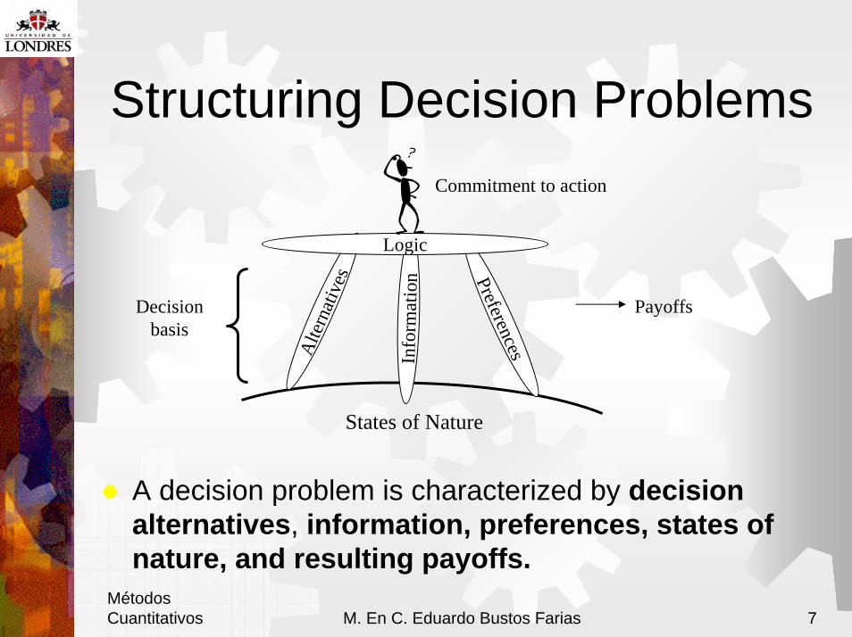
A decision problem is characterized by decision alternatives, information, preferences, states of nature, and resulting payoffs.


Structuring the Decision Problems

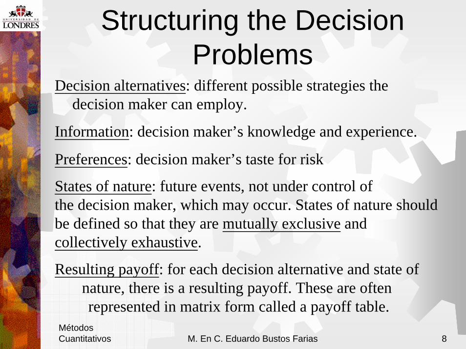
Decision alternatives: different possible strategies the decision maker can employ.

Information: decision maker’s knowledge and experience.

Preferences: decision maker’s taste for risk

States of nature: future events, not under control of the decision maker, which may occur. States of nature should be defined so that they are mutually exclusive and collectively exhaustive.

Resulting payoff: for each decision alternative and state of nature, there is a resulting payoff. These are often represented in matrix form called a payoff table.


An Investment ExampleTom has inherited $1000 from a distant relative. He decided to invest the $1000 for a year to get some hands-on investment experience before graduating from college.

Tom’s broker has selected three potential investments she believes would be appropriate for Tom: a mutual fund, a growth stock, and a certificate of deposit. Given the small amount of money that Tom has for investment, the broker suggests Tom to pick one out of the three investments.

Which investment should Tom pick?


Decision Making under Uncertainty

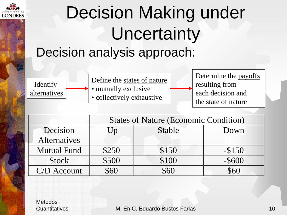
Decision analysis approach:

Identify alternativesIdentify

alternatives

Define the states of nature• mutually exclusive• collectively exhaustive

Define the states of nature• mutually exclusive• collectively exhaustive

Determine the payoffsresulting fromeach decision and the state of nature

Determine the payoffsresulting fromeach decision and the state of nature

States of Nature (Economic Condition)Decision

Alternatives Up Stable Down

Mutual Fund $250 $150 -$150Stock $500 $100 -$600

C/D Account $60 $60 $60


Decision Making under Uncertainty -without Probability Information

If the decision maker does not know with certainty which state of nature will occur, then he is said to be doing decision making under uncertaintyThree commonly used criteria for decision making under uncertainty when probability information regarding the likelihood of the states of nature is unavailable are:

1. The optimistic approach2. The conservative approach3. The minimax regret approach


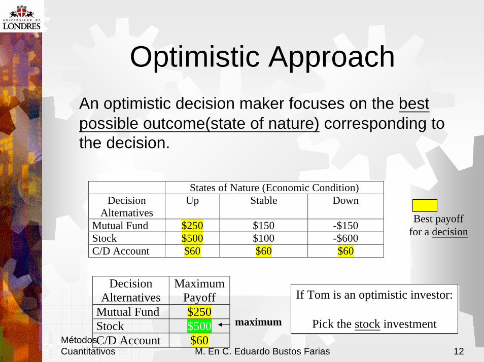
Optimistic ApproachAn optimistic decision maker focuses on the best possible outcome(state of nature) corresponding to the decision.


AlternativesUp Stable Down

Mutual Fund $250 $150 -$150Stock $500 $100 -$600C/D Account $60 $60 $60

DecisionAlternatives

MaximumPayoff

Mutual Fund $250Stock $500C/D Account $60

maximum

If Tom is an optimistic investor:

Pick the stock investment

If Tom is an optimistic investor:

Pick the stock investment

Best payofffor a decision


Optimistic Approach

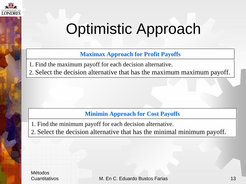
1. Find the maximum payoff for each decision alternative.2. Select the decision alternative that has the maximum maximum payoff.1. Find the maximum payoff for each decision alternative.2. Select the decision alternative that has the maximum maximum payoff.

Maximax Approach for Profit PayoffsMaximax Approach for Profit Payoffs

1. Find the minimum payoff for each decision alternative.2. Select the decision alternative that has the minimal minimum payoff.1. Find the minimum payoff for each decision alternative.2. Select the decision alternative that has the minimal minimum payoff.

Minimin Approach for Cost PayoffsMinimin Approach for Cost Payoffs


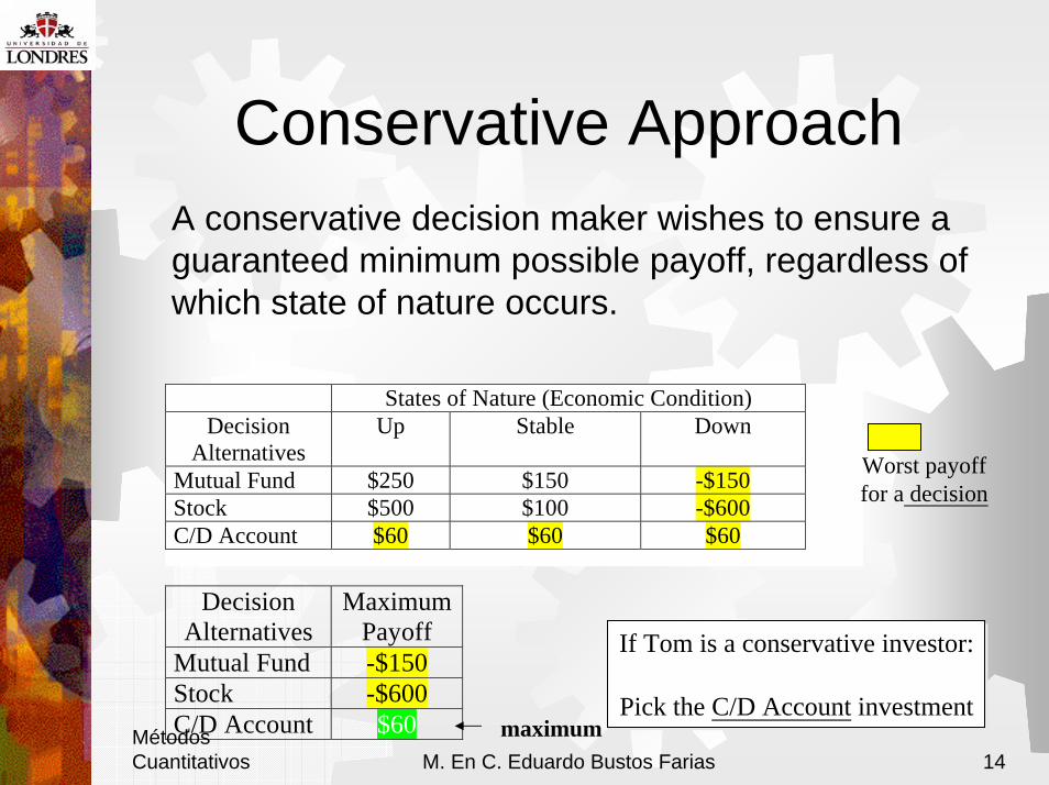
Conservative ApproachA conservative decision maker wishes to ensure a guaranteed minimum possible payoff, regardless of which state of nature occurs.




Worst payofffor a decision


MaximumPayoff

Mutual Fund -$150Stock -$600C/D Account $60 maximum

If Tom is a conservative investor:

Pick the C/D Account investment

If Tom is a conservative investor:

Pick the C/D Account investment


Conservative Approach

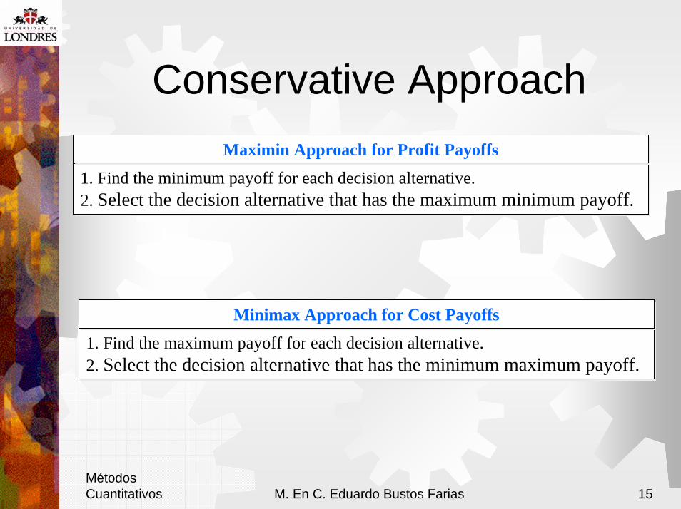
1. Find the minimum payoff for each decision alternative.2. Select the decision alternative that has the maximum minimum payoff.1. Find the minimum payoff for each decision alternative.2. Select the decision alternative that has the maximum minimum payoff.

Maximin Approach for Profit PayoffsMaximin Approach for Profit Payoffs

1. Find the maximum payoff for each decision alternative.2. Select the decision alternative that has the minimum maximum payoff.1. Find the maximum payoff for each decision alternative.2. Select the decision alternative that has the minimum maximum payoff.

Minimax Approach for Cost PayoffsMinimax Approach for Cost Payoffs


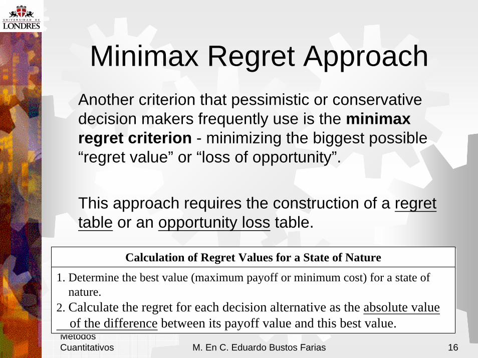
Minimax Regret ApproachAnother criterion that pessimistic or conservative decision makers frequently use is the minimaxregret criterion - minimizing the biggest possible “regret value” or “loss of opportunity”.

This approach requires the construction of a regret table or an opportunity loss table.

Calculation of Regret Values for a State of NatureCalculation of Regret Values for a State of Nature

1. Determine the best value (maximum payoff or minimum cost) for a state of nature.

2. Calculate the regret for each decision alternative as the absolute valueof the difference between its payoff value and this best value.




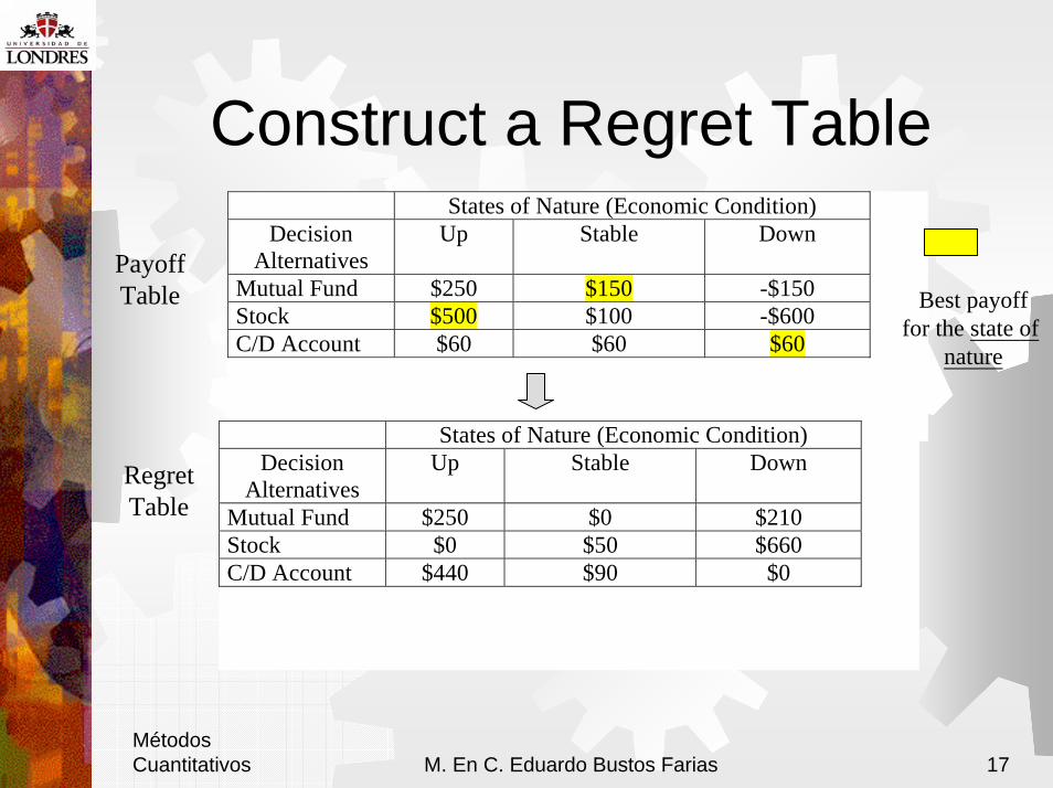
Construct a Regret TableStates of Nature (Economic Condition)


Up Stable Down




Mutual Fund $250 $0 $210Stock $0 $50 $660C/D Account $440 $90 $0

PayoffTable

RegretTable

Best payofffor the state of

nature


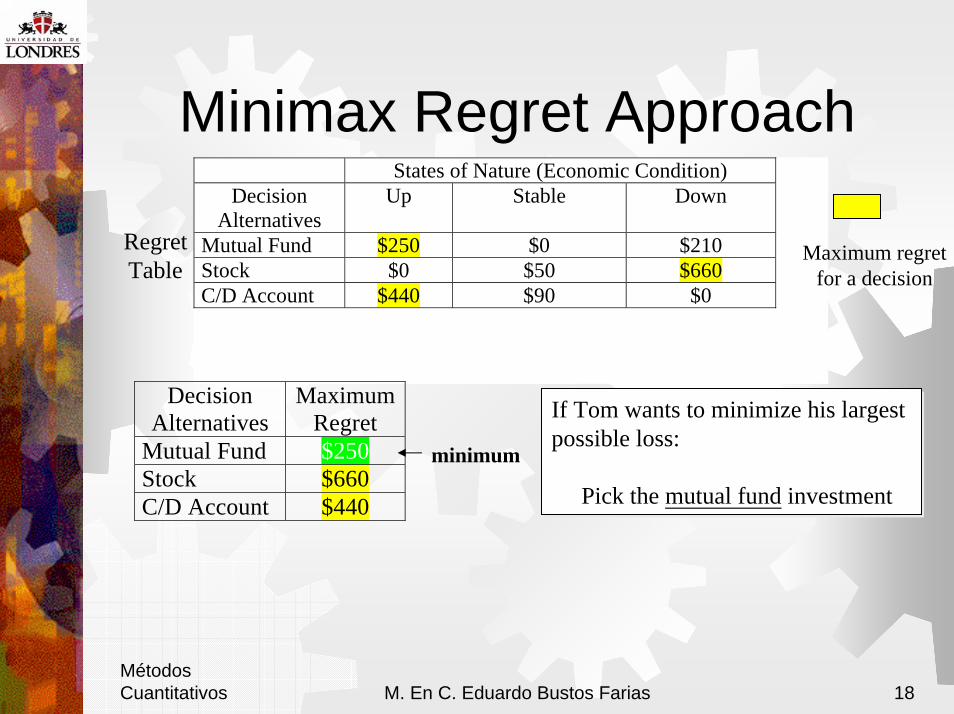
Minimax Regret ApproachStates of Nature (Economic Condition)


Up Stable Down

Mutual Fund $250 $0 $210Stock $0 $50 $660C/D Account $440 $90 $0

RegretTable

Maximum regretfor a decision


MaximumRegret

Mutual Fund $250Stock $660C/D Account $440

minimum

If Tom wants to minimize his largest possible loss:

Pick the mutual fund investment

If Tom wants to minimize his largest possible loss:

Pick the mutual fund investment


Minimax Regret Approach



3. Find the maximum regret for each decision alternative.4. Select the decision alternative that has the minimum maximum regret.



3. Find the maximum regret for each decision alternative.4. Select the decision alternative that has the minimum maximum regret.

Minimax Regret ApproachMinimax Regret Approach


What If Probability Information is Available?

Federal Reserve predicts that the economy will go up with probability 40%, stay stable with probability 50%, and go down with probability 10%.

How might Tom use this information?


We Encode Our Uncertainty Using Probability

Uncertainty comes from our lack of knowledge

Probability allows us to “speak precisely about our ignorance”Instead of “the probability is …” say “I assign the probability ... to…”

Your probability changes as your knowledge changesAlways condition probabilities on your background state of information - all your knowledge and experience

We condition A on B when we think about A given that B happened


Expected Value ApproachIf a probability estimate for the occurrence of each state of nature is available, one may use the expected value approach.1. Find the expected payoff for each decision alternative.

- multiply the probability for each state of nature by the associated returnand then sum these product.

2. Select the decision alternative that has the best expected payoff.

1. Find the expected payoff for each decision alternative.- multiply the probability for each state of nature by the associated returnand then sum these product.

2. Select the decision alternative that has the best expected payoff.

Expected Value ApproachExpected Value Approach

States of Nature (Economic Condition) Decision

Alternatives Up Stable Down Expected Value

(EV) Mutual Fund $250 $150 -$150 =.4*250+.5*150+.1*-150 = 160 Stock $500 $100 -$600 =.4*500+.5*100+.1*-600 = 190 C/D Account $60 $60 $60 =.4*60+.5*60+.1*60 = 60 Probability 0.4 0.5 0.1


Conditional ProbabilityGiven events A and B, the probability that A happens

given that we know B happens can be calculated by:

Equivalently

{A|B}: A given B{A∩B}: A joint B

( ) ( )BPBAPBAP )(| ∩

=

( ) ( )BPBAPBAP )|(=∩


Prior and Posterior Probabilities -Bayesian Analysis

Bayesian Analysis

Prior ProbabilityPrior Probability additionalInformationadditional

InformationPosterior

ProbabilityPosterior

Probability

Prior Probability: Prior to obtaining additional information, the probability estimates for the state of nature

Posterior Probability:Through Bayesian analysis, prior probabilities are revised, the outcome is posterior probability


Bayes TheoremThe famous Bayes’ Theorem:

Given events B and A1, A1, A1, …, An, where A1, A1, A1, …, An are mutually exclusive and collectively exhaustive, posterior probabilities Pr(Ai|B) can be found by:

P(Ai): prior probabilityP(Ai|B): posterior probability

( ) ( )( )

( )( ) ( ) ( )

)()|(...)()|()()|()()|(

...|

2211

21

nn

ii

n

iii

APABPAPABPAPABPAPABP

ABPABPABPABP

BPABPBAP

+++=

∩++∩+∩∩

=∩

=


Decision Tree ApproachA decision tree is a chronological representation of the decision problem:

: decision node: state-of-nature node

: branches leaving decision node represent different decision alternatives

: branches leaving state-of-nature node represent the different states of nature


Construct a Decision TreeRoot of tree: corresponds to the present

time; tree is constructed outward into future

The end of each limb of a tree: payoffs attained from the series of branches making up that limb.


Construct a New Decision Tree


What If More Information Can Be Obtained?

Tom has learned that, for only $50, he can receive the results of a noted economist’s forecast, which predicates “up,” “stable,” and “down” for the upcoming year. The economist offered the following verifiable statistics regarding the result of his model:When economy went up, his forecast predicted “up” 80% of the time, “stable” 10% of the time,and “down” 10% of the time.

When economy was stable, his forecast predicted “up” 30% of the time, “stable” 60% of the time,and “down” 10% of the time.

When When economy went down, his forecast predicted “up” 0% of the time, “stable” 10% of the time,and “down”90% of the time.


Conditional ProbabilityShould Tom purchase the forecast information

from the economist?Using probability language, how is the performance of theeconomist’s forecasts?When the economy went up, the economist predictedPr(“up”|up)=0.8 Pr(“stable”|up)=0.1 Pr(“down”|up)=0.1

When the economy stayed stable, the economist predictedPr(“up”|stable)=0.3 Pr(“stable”|stable)=0.6 Pr(“down”|stable)=0.1

When the economy went down, the economist predictedPr(“up”|down)=0 Pr(“stable”|down)=0.1 Pr(“down”|down)=0.9


Bayesian Analysis - Tabular Approach

″up″ economical forecast for Tom:

State ofNatureSi

PriorProbabilityP(Si)

ConditionalprobabilityP("up"|Si)

Joint ProbabilityP(Si and "up")

PosteriorProbabilityP(Si|"up")

up 0.4 0.8 0.32 0.68stable 0.5 0.3 0.15 0.32down 0.1 0 0 0.00

P(get "up")= 0.47

Step1: Fill in Prior probabilities P(Si) and conditionalprobabilities P(″up″|Si)

Step 2: Calculate joint probabilities P(″up″∩Si)= P(″up″|Si)×P(Si)

Step 3: Sum the Joint Probability Column to calculate the marginal probability P(″up″)

Step 4: Calculate the posterior probability using Bayes Theorem:

P(Si|″up″)= P(″up″∩Si)/ P(″up″)



State ofNatureSi


ConditionalprobabilityP("stable"|Si)

Joint ProbabilityP("stable"and Si)

PosteriorProbabilityP(Si|"stable")

up 0.4 0.1 0.04 0.11stable 0.5 0.6 0.3 0.86down 0.1 0.1 0.01 0.03

P(get "stable")= 0.35

″stable″ economical forecast for Tom:

″down″ economical forecast for Tom:

State ofNatureSi


ConditionalprobabilityP("down"|Si)

Joint ProbabilityP(Si and"down")

PosteriorProbabilityP(Si|"down")

up 0.4 0.1 0.04 0.22stable 0.5 0.1 0.05 0.28down 0.1 0.9 0.09 0.50

P(get "down")= 0.18



Posterior Probability Table

Nature\Forecast Up Stable DownAlternativ

esMutualFund

Stock C/DAccount

Up 0.68 0.11 0.22 Up $250 $500 $60Stable 0.32 0.86 0.28 Stable $150 $100 $60Down 0 0.03 0.5 Down ($150) ($600) $60

Forecast Up Stable DownMutual Fund 218 152 22Stock 372 123 -162C/D Account 60 60 60Prob(get " ")= 0.47 0.35 0.18 238.84

48.84

ExpectedPayoff Under

SampleInformation

Posterior Probability Table Payoff Table

EVSI (expected Value of SampleInformation)=

Sumproduct(Posterior Prob. * Payoff)


Expected Value of Sample Information

Expected Value with Sample Information about the States of NatureEVwSI = $238.8

Expected Value without Sample Information about the States of NatureEVwoSI = $190 = result from the expected value approach

Expected Value of Sample Information (EVSI)EVSI = | EVwSI − EVwoSI| = $238.8 − $190 = $48.8(additional expected payoff possible through knowledge of the sample information)


Expected Value of Perfect Information

If Tom knew in advance how the economic situation would be in a year, what his optimal decision would be?

There is a 40% probability that this perfect information will indicate an up economic situation and Tom will invest in stock and earn $500.

Similarly, with 50% probability, the perfect information will indicate a stable economy and Tom will invest in mutual fund and earn $150.

With 10% probability, the perfect information will indicate a down economy and Tom will invest in C/D account and earn $60.

If Tom knew in advance theeconomic situation would be

His OptimalDecision would be With a payoff of

Up Stock $500Stable Mutual fund $150Down CD $60



Expected Value with Perfect Information about the States of NatureEVwPI = $500×0.4+$150×0.5+$60 ×0.1=$281

Expected Value without Perfect Information about the States of NatureEVwoPI = $190 = result from the expected

value approach

Expected Value of Perfect InformationEVPI = | EVwPI − EVwoPI| = $281 − $190 =

$91



1. Determine the best payoff corresponding to each state of nature.2. Compute the expected value of these best payoffs (EVwPI).3. Compute the expected value without the perfect information (EVwOPI)

using the expected value approach.4. EVPI = | EVwPI− EVwoPI|

1. Determine the best payoff corresponding to each state of nature.2. Compute the expected value of these best payoffs (EVwPI).3. Compute the expected value without the perfect information (EVwOPI)

using the expected value approach.4. EVPI = | EVwPI− EVwoPI|

Expected Value of Perfect InformationExpected Value of Perfect Information

EVPI is the increase in the expected payoff that would result ifone knew with certainty which state of nature would occur.

The EVPI provides an upper bound on the expected value of any sample or survey information.


Efficiency of Sample Information

Efficiency of sample information

(Investment example: efficiency = $48.8/$91 = 53.6%) WHY < 1?

• EVPI provides an upper bound for the EVSI, efficiency of sample information is always a number between 0 and 1. WHY?

EVPIEVSI

=n Informatio Sample of Efficienty


SummaryDecision Analysis is a coherent procedure to decision making

Basis for decision makingAlternativesinformationpreferences

Basis for decision makingAlternativesinformationpreferences

Optimistic approachConservative approach

Minimax regret approach

Optimistic approachConservative approach

Minimax regret approach

Bayes Theoremto revise probabilities

prior probability⇓

posterior probability

Bayes Theoremto revise probabilities

prior probability⇓

posterior probability

Expected value approachDecision tree approach

Expected value approachDecision tree approach

No probabilityinformation

Probability information

Sample information




DECISION ANALYSIS:DECISION TREES AND

SENSITIVITY


Elements of a Decision Analysis


Background InformationSciTools Incorporated specializes in scientific instruments and has been invited to make a bid on a government contract.The contract calls for a specific number of these instruments to be delivered during the coming year.SciTools estimates that it will cost $5000 to prepare a bid and $95,000 to supply the instruments.


Background Information --continued

On the basis of past contracts, SciTools believes that the possible low bids from the competition (if there is competition) and the associated probabilities are:

In addition, they believe there is a 30% chance that there will be no competing bids.

Data for Bidding ExampleLow Bid ProbabilityLess than $115,000 0.2Between $115,000 and $120,000 0.4Between $120,000 and $125,000 0.3Greater than $125,000 0.1


Decision Making ElementsAlthough there is a wide variety of contexts in decision making, all decision making problems have three elements:

the set of decisions (or strategies) available to the decision makerthe set of possible outcomes and the probabilities of these outcomea value model that prescribes results, usually monetary values, for the various combinations of decisions and outcomes.

Once these elements are known, the decision maker can find an “optimal” decision.


SciTools’ ProblemThere are three elements to SciTools’problem.The first element is that they have two basic strategies - submit a bid or do not submit a bid.

If they decide to submit a bid they must determine how much they should bid.The bid must be greater than $100,000 for SciTools to make a profit.The Bidding Data would probably persuade SciTools to bid either $115,000, $120,000, $125,000 or a number in between these.


SciTools’ Problem --continued

The next element involves the uncertain outcomes and their probabilities.

We have assumed that SciTool knows exactly how much it will cost to prepare the bid and supply the instruments if they win the bid. In reality these are probably estimates of the actual cost.Therefore, the only source of uncertainty is the behavior of the competitors - will they bid and, if so, how much?The behavior of the competitors depends on how many competitors are likely to bid and how the competitors assess their costs of supplying the instruments.



From past experience SciTools is able to predict competitor behavior, thus arriving at the 30% estimate of the probability of no competing bids.

The last element of the problem is the value model that transforms decisions and outcomes into monetary values for SciTools.

The value model in this example is straightforward but in other examples it is often complex.If SciTools decides right now not to bid, then its monetary values is $0 - no gain, no loss.



If they make a bid and are underbid by a competitor, then they lose $5000, the cost of preparing the bid.If they bid B dollars and win the contract, then they make a profit of B - $100,000; that is, B dollars for winning the bid, less $5000 for preparing the bid, less $95,000 for supplying the instruments.It is often convenient to list the monetary values in a payoff table.


SciTools’ Payoff TablesPayoff Table for SciTools Bidding Example

SciToolsBidNo Bid115120125Probability 0.3 0.7(0.2) 0.7(0.4) 0.7(0.3) 0.7(0.1)

No Bid

<115 >115, <120

>120, <125 >125

0152025

Competitors’ Lowest Bid ($1000s)

0 0 0 015 15

20-5

-5-5

-5-5-5

152025

Probability in parenthesis means the probability of competitors lowest bid if they bid. P(Ai|B)= P(Ai B) / P(B)So, what are the P(Ai B)s for all i ? Often it is possible to simplify the payoff tables to better understand the essence of the problem. SciTools care only whether they win the contract or not. An alternative payoff table for SciTools is shown on the next slide.


Alternative Payoff Table for SciTools Bidding Example

Monetary Value

SciTools Bids($2000)

No Bid

115

120

125

SciTools Wins SciToolsLoses

Probability That ScitTools Wins

NA 0 0.00

-5 0.86=0.3+0.7(0.4+0.3+0.1)

0.58=0.3+0.7(0.3+0.1)

0.37=0.3+0.7*0.1

-5

-5

15

20

25

Decision tree construction….


Risk Profiles for SciToolsA risk profile simply lists all possible monetary values and their corresponding probabilities.From the alternate payoff table we can obtain risk profiles for SciTools.

For example, if SciTools bids $120,000 there are two possibly monetary values, a profit of $20,000 or a loss of $5000, and their probabilities are 0.58 and 0.42, respectively.

Risk profiles can be illustrated on a bar chart. There is a bar above each possible monetary value with height proportional to the probability of that value.


Expected Monetary ValuesWe still don’t know which choice SciTools should make. If SciTools knew what the competitors would do the decision would be easy. However, the decision must be made before this uncertainty is resolved.A common way used to make the choice is to calculate the expected monetary value (EMV) of each alternative and then choose the alternative with the largest EMV. EMV is a weighted average of the possible monetary values, weighted by their probabilities.


SciTools’ EMVsEMVs for SciTools Bidding ExampleAlternative EMV

CalculationEMV

No BidBid $115,000

Bid $120,000

Bid $125,000

0(1) $015,000(0.86) + (-5000)(0.14)

$12,200

$9500

$6100

20,000 (0.58) + (-5000)(0.42)

25,000(0.37) + (-5000)(0.63)

What exactly does the EMV mean?

It means that if SciTools were to enter many “gambles”like this, where on each gamble the gains, losses and probabilities were the same, then on average it would win $12,200 per gamble.


Decision TreesSo far in this example we have gone through most of the steps in solving SciTools’ problem.All of this can be done efficiently using a graphical tool called a decision tree.To understand SciTools’ and other decision trees we need to know the following conventions that have been established for decision trees.


Decision Tree Conventions1. Decision trees are composed of nodes

(circles, squares and triangles) and branches (lines).

2. The nodes represent points in time. A decision node(a square) is a time when the decision maker makes a decision. A probability node (a circle) is a time when the result of an uncertain event becomes known. An end node (a triangle) indicates that the problem is completed - all decisions have been made, all uncertainty have been resolved and all payoffs have been incurred.


Decision Tree Conventions --continued

3. Time proceeds from left to right. This means that branches leading into a node (from the left) have already occurred. Any branches leading out of a node (to the right) have not yet occurred.

4. Branches leading out of a decision node represent the possible decisions; the decision maker can choose the preferred branch. Branches leading out of probability nodes represent the possible outcomes of uncertain events; the decision maker has no control over which of these will occur.



5. Probabilities are listed on probability branches. These probabilities are conditional on the events that have already been observed (those to the left). Also, the probabilities on branches leading out of any particular probability node must sum to 1.

6. Individual monetary values are shown on the branches where they occur, and cumulative monetary values are shown to the right of the end nodes. (Two values are often found to the right of each node: the top one is the probability of getting to that end node, and the bottom one is the associated monetary value).


SciTools’ Decision tree



This decision tree illustrates these conventions for a single-stage decision problem, the simplest type of decision problem.In a single-stage decision problem all decisions are made first, and then all uncertainty is resolved.Later we will see multistage decision problems, where decisions and outcomes alternate.Once a decision tree has been drawn and labeled with the probabilities and monetary values, it can be solved easily.


Folding Back ProcedureThe solution for the decision tree is on the next slide.The solution procedure used to develop this result is called folding back on the tree. Starting at the right on the tree and working back to the left, the procedure consist of two types of calculations.

At each probability node we calculate EMV and write it below the name of the node.At each decision node we find the maximum of the EMVs and write it below the node name.

After folding back is completed we have calculated EMVs for all nodes.


Result of Folding Back to Obtain Optimal Decision


The PrecisionTree Add-InDecision trees present a challenge for Excel. The PrescisionTree Add-in makes the process relatively straightforward.This add-in enables us to build and label a decision tree, but it performs the folding-back procedure automatically and then allows us to perform the folding back procedure automatically and then allows us to perform sensitivity analysis on key input parameters.


The PrecisionTree Add-In --continued

The first things you must do to use PrecisionTree is to “add it in”. Install the Palisade’s Decision Tools suite with the Setup program on the CD-ROM. Then to run PrecisionTree, there are three options:

If Excel is not currently running , you can launch Excel and PrecisionTree by clicking on the Windows Start button and selecting the PrecisionTree item.

If Excel is currently running, the procedure in the previous bullet will launch PrecisionTree on top of Excel.

If Excel is already running and the Desktop Tools toolbar (shown on the next slide) is showing, you can start PrecisionTree by clicking on its icon.


SCITOOLS.XLSThis file contains the results of the PrecisionTree procedure, but you should work through the steps on your own, starting with a blank spreadsheet.You’ll now when PrecisionTree is ready for use when you see its toolbar.



Using PrecisionTree: Inputs. Enter the inputs shown in columns A and B of this table.New tree. Click on the new tree button (the far left button) on the PrecisionTree toolbar, and then click on any cell below the input section to start a new tree. Click on the name box of this new tree to open a dialog box. Type in a descriptive name for the tree, as shown on the next slide.



Decision nodes and branches. From here on, keep the finished tree shown earlier in mind. This is the finished product toward which we’re building. To obtain decision nodes and branches, click on the (only) triangle end node to open the dialog box shown on the next slide.




We’re calling this decision “Bid?” and specifying that there are two possible decisions. The tree expands as shown here.

The boxes that say “branch” show the default labels for these branches. Click on either of the to open another dialog box where you can provide a more descriptive name for the branch. Do this to label the two branches “No” and “Yes.”Also, you can enter the immediate payoff/cost for either branch right below it. Since there is a $5000 cost of bidding, enter the formula =BidCost right below the “Yes” branch in cell B19. The tree should now appear as shown on the next slide.



More decision branches. The top branch is completed; if SciTools does not bid, there is nothing left to do. So click on the bottom end node, following SciTools’ decision to bid, and proceed as in the previous step to add and label the decision node and three decision branches for the amount to bid. The tree to this point should appear as shown on the next slide. Note that there are no monetary values below these decision branches because no immediate payoffs or costs are associated with the bid amount decision.




Probability nodes and branches. We now need a probability node and branches from the rightmost end nodes to capture the competition bids. Click on the top one of these end nodes to bring up the same dialog box as shown below. Now, however, click on the red circle box to indicate that this is a probability node. Label it “Any competing bid?”, specify two branches, and click on OK. Then label the two branches “No” and “Yes”. Next, repeat this procedure to form another probability node following the “Yes” branch, call it “Win bid?”, and label its branches as shown on the next slide.




Copying probability nodes and branches. You could build the next node and branches or take advantage of PrecisionTree’s copy and paste function. Labeling probability branches. You should now have the decision tree as shown on the next slide. The structure is the same as the finished model but the monetary values are not correct. First enter the probability of no competing bid in cellD18 with the formula =PrNoBid and enter its complement in cell D24 with the formula =1-D18. Next, enter the probability that SciTools wins the bid in cell E22 with the formula =SUM(B10:B12) and enter its complement in cell E26 with the formula =1-E22.




For the monetary values, enter the formula =115000-ProdCost in the two cells, D19 and E23, where SciTools wins the contract.Enter the other formulas on probability branches. Using the previous step and the final decision tree as a guide, enter formulas for the probabilities and monetary values on the other probability branches, that is, those following the decision to bid $120,000 or $125,000.

We’re finished! The completed tree shows the best strategy and its associated EMV.


Risk Profile of Optimal Strategy

Once the decision tree is completed, PrecisionTree has several tools we can use to gain more information about the decision analysis.First we see a risk profit and other information about the optimal decision.To do so, click on the fourth button from the left on the PrecisionTree toolbar. Then fill in the resulting dialog box shown on the next slide. The Policy Suggestion option allows us to see only that part of the tree that corresponds to the best decision, also shown on the next slide.



Risk Profile of Optimal Strategy -- continued

The Risk Profile option allows us to see a graphical risk of the optimal decision. As the risk profile shown on the next slide shows, there are only two possible monetary outcomes if SciTools bids $115,000.This graphical information is even more useful when there are a larger number of possible monetary outcomes.



Sensitivity AnalysisWe have already stressed the importance of the follow-up sensitivity analysis for any decision problem, and PrecisionTree makes this relatively easy to perform.First we enter any values not the input cells and watch how the tree changes. But we can get more systematic information by clicking on PrecisionTree’s sensitivity button. This brings up the dialog box shown on the next slide. It requires EMV cell to analyze at the top and one or more input cells in the middle.



Sensitivity Analysis --continued

The cell to analyze is usually the EMV cell at the far left of the decision tree but it can be any EMV cell.Next, for any input cell such as the production cost cell, we enter a minimum value, a maximum value, a base value, and a step size.When we click Run Analysis, PrecisionTree varies each of the specified inputs and presents the results in several ways in a new Excel file with Sensitivity, Tornado, and Spider Graph sheets.



The Sensitivity sheet includes several charts, a typical one of which appears here. This shows how the EMV varies with the production cost for both of the original decisions. This type of graph is useful for seeing whether the optimal decision changes over the range of input variable.



The Tornado sheet shows how sensitive the EMV of the optimal decision is to each of the selected inputs over the ranges selected. Here we see that production cost has the largest effect on EMV, and bid cost has the smallest effect.



Finally, the Spider Chart shows how much the optimal EMV varies in magnitude for various percentage changes in the input variables. We again see that the production cost has a relatively largest effect, whereas the other two inputs have relatively small effects.



Each time we click on the sensitivity button, we can run a different sensitivity analysis.An interesting option is to run a two-way analysis. Then we see how the selected EMV varies as each pair of inputs vary simultaneously.A typical result is shown on the next slide. For each of the possible values of production cost and probability of no competitor bid, this chart indicates which bid amount is optimal.



As we see, the optimal bid amount remains $115,000 unless the production cost and the probability of no competing bid are both large. Then it becomes optimal to bid $125,000.


Bayes’ Rule


Background InformationIf an athlete is tested for certain type of drug use, the test will come out either positive or negative.However, these tests are never perfect. Some athletes who are drug-free test positive (false positives) and some who are drug users test negative (false negatives). We will assume that

5% of all athletes use drugs

8% of all tests on drug-free athletes yield false positives

3% of all tests on drug users yield false negatives.

The question then is what we can conclude from a positive or negative test result.


SolutionLet D and ND denote that a randomly chosen athlete is or is not a drug user, and let T+ and T- indicate a positive or negative test result.We know the following probabilities

First, since 5% of all athletes are drug users, we know that P(D) = 0.05 and P(ND) = 0.95. These are called prior probabilities because they represent the chance that an athlete is or is not a drug user prior to the results of a drug test.


Solution -- continuedSecond, from the information on drug test accuracy, we know the conditional probabilities P(T+|ND) = 0.08 and P(T-|D)= 0.03.But a drug-free athlete either tests positive or negative, and the same is true for a drug user. Therefore, P(T-|ND) = 0.92 and P(T+|D) = 0.97.These four conditional probabilities of test results given drug user status are often called the likelihoods of the test results.

Given these priors and likelihoods we want posterior probabilities such as P(D|T+) or P(ND|T-).


Solution -- continuedThese are called posterior probabilitiesbecause they are assessed after the drug test results. This is where Baye’s rule enters.Bayes’ Rule says that a typical posterior probability is a ratio. The numerator is a likelihood times a prior, and the denominator is the sum of likelihoods times priors.


DRUGBAYES.XLS

This file shows how easy it is to implement Bayes’ rule in a spreadsheet.The given priors and likelihoods are listed in the ranges B5:C5 and B9:C10.


CalculationsWe calculate the products of likelihoods and priors in the range B15:C16. The formula in cell B15 is=B$5*B9 and it is copied to the rest of B15:C16 range.Their row sums are calculated in the range D15:D16. These represent the unconditional probabilities of the two possible results. They are also the denominator of Bayes’ rule.Finally we calculate the posterior probabilities in the range B21:C22. The formula in B21 is =B15/$D15 and it is copied to the rest of the range B21:C22.


Resulting ProbabilitiesA negative test result leaves little doubt that the athlete is drug-free; this probability is 0.996.A positive test result leaves a lot of doubt of whether the athlete is drug-free. The probability that the athlete uses drugs is 0.617.Since only 5% of athletes use drugs it takes a lot of evidence to convince us otherwise. This plus the fact that the test produces false positives means the athletes that test positive still have a decent chance of being drug-free.

Documents

DECISION ANALYSIS: INTRODUCTION - Angelfire: … · 2005-09-12 · Métodos Cuantitativos M. En C. Eduardo Bustos Farias 2 Agenda Decision analysis in general Structuring decision