Decision Analysis

Ch. 822C:145 AI

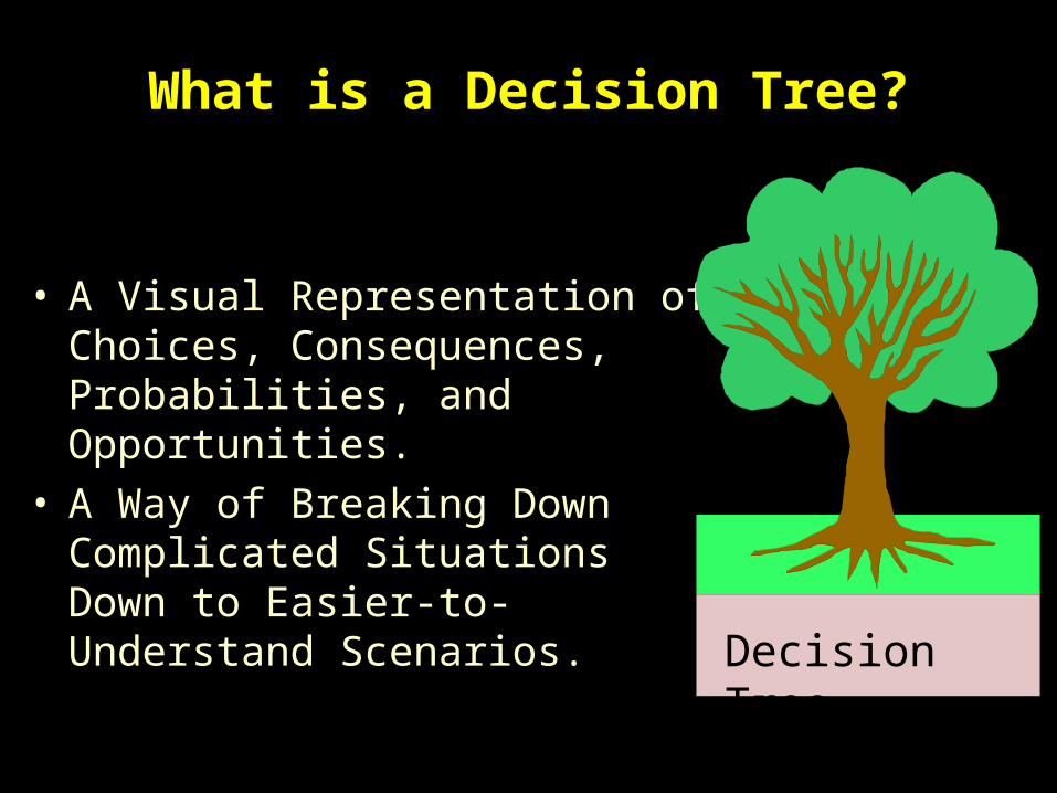
What is a Decision Tree?

• A Visual Representation of Choices, Consequences, Probabilities, and Opportunities.

• A Way of Breaking Down Complicated Situations Down to Easier-to-Understand Scenarios.

Decision Tree

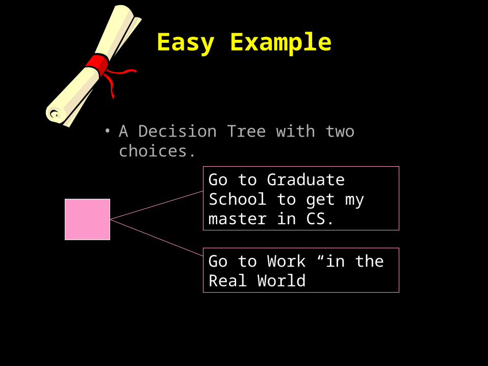
Easy Example

• A Decision Tree with two choices.

Go to Graduate School to get my master in CS.

Go to Work “in the Real World”

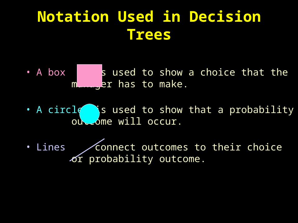
Notation Used in Decision Trees

• A box is used to show a choice that the manager has to make.

• A circle is used to show that a probability outcome will occur.

• Lines connect outcomes to their choice or probability outcome.

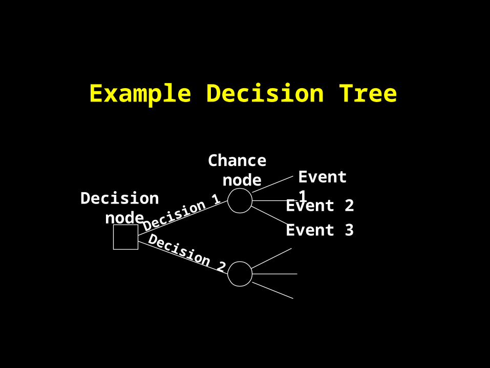
Example Decision Tree

Decision node

Chance node

Decision 1

Decision 2

Event 1

Event 2

Event 3

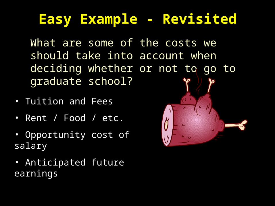
Easy Example - Revisited

What are some of the costs we should take into account when deciding whether or not to go to graduate school?

• Tuition and Fees

• Rent / Food / etc.

• Opportunity cost of salary

• Anticipated future earnings

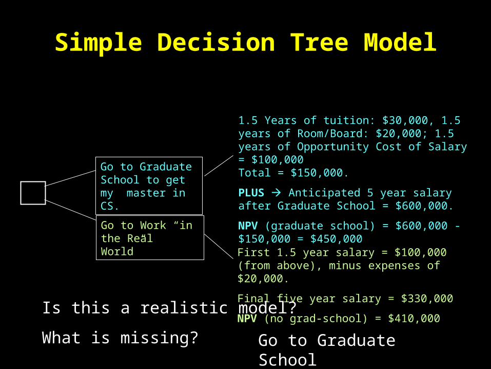
Simple Decision Tree Model

Go to Graduate School to get my master in CS.

Go to Work “in the Real World”

1.5 Years of tuition: $30,000, 1.5 years of Room/Board: $20,000; 1.5 years of Opportunity Cost of Salary = $100,000 Total = $150,000.

PLUS Anticipated 5 year salary after Graduate School = $600,000.

NPV (graduate school) = $600,000 - $150,000 = $450,000

First 1.5 year salary = $100,000 (from above), minus expenses of $20,000.

Final five year salary = $330,000

NPV (no grad-school) = $410,000Is this a realistic model?

What is missing? Go to Graduate School

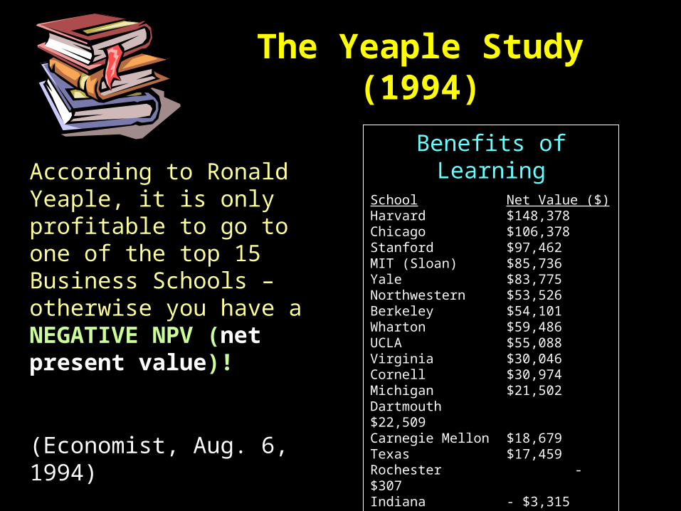
The Yeaple Study (1994)

According to Ronald Yeaple, it is only profitable to go to one of the top 15 Business Schools – otherwise you have a NEGATIVE NPV (net present value)!

(Economist, Aug. 6, 1994)

Benefits of LearningSchool Net Value ($)Harvard $148,378Chicago $106,378Stanford $97,462MIT (Sloan) $85,736Yale $83,775Northwestern $53,526Berkeley $54,101Wharton $59,486UCLA $55,088Virginia $30,046Cornell $30,974Michigan $21,502Dartmouth $22,509Carnegie Mellon $18,679Texas $17,459Rochester - $307Indiana - $3,315North Carolina - $4,565Duke - $17,631NYU - $3,749

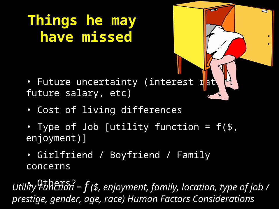
Things he may have missed

• Future uncertainty (interest rates, future salary, etc)

• Cost of living differences

• Type of Job [utility function = f($, enjoyment)]

• Girlfriend / Boyfriend / Family concerns

• Others?

Utility Function = f ($, enjoyment, family, location, type of job / prestige, gender, age, race) Human Factors Considerations

Example – Joe’s Garage

Joe’s garage is considering hiring another mechanic. The mechanic would cost them an additional $50,000 / year in salary and benefits. If there are a lot of accidents in Iowa City this year, they anticipate making an additional $75,000 in net revenue. If there are not a lot of accidents, they could lose $20,000 off of last year’s total net revenues. Because of all the ice on the roads, Joe thinks that there will be a 70% chance of “a lot of accidents” and a 30% chance of “fewer accidents”. Assume if he doesn’t expand he will have the same revenue as last year.

Draw a decision tree for Joe and tell him what he should do.

Example - Answer

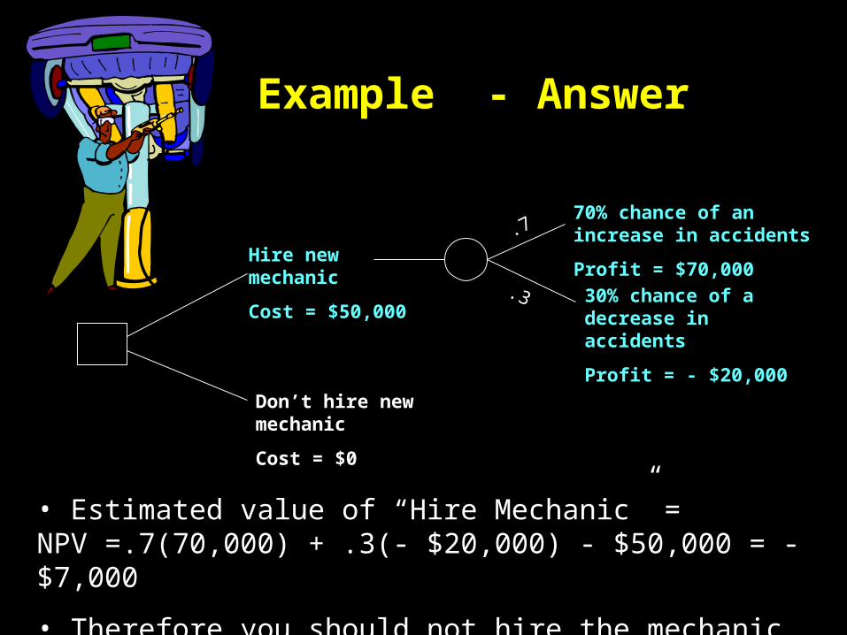
Hire new mechanic

Cost = $50,000

Don’t hire new mechanic

Cost = $0

70% chance of an increase in accidents

Profit = $70,000

30% chance of a decrease in accidents

Profit = - $20,000

• Estimated value of “Hire Mechanic” = NPV =.7(70,000) + .3(- $20,000) - $50,000 = - $7,000

• Therefore you should not hire the mechanic

.7

.3

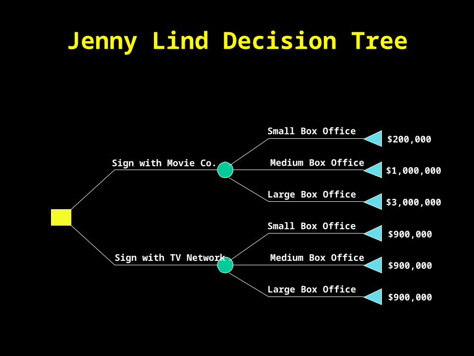
Problem: Jenny Lind

Jenny Lind is a writer of romance novels. A movie company and a TV network both want exclusive rights to one of her more popular works. If she signs with the network, she will receive a single lump sum, but if she signs with the movie company, the amount she will receive depends on the market response to her movie. What should she do?

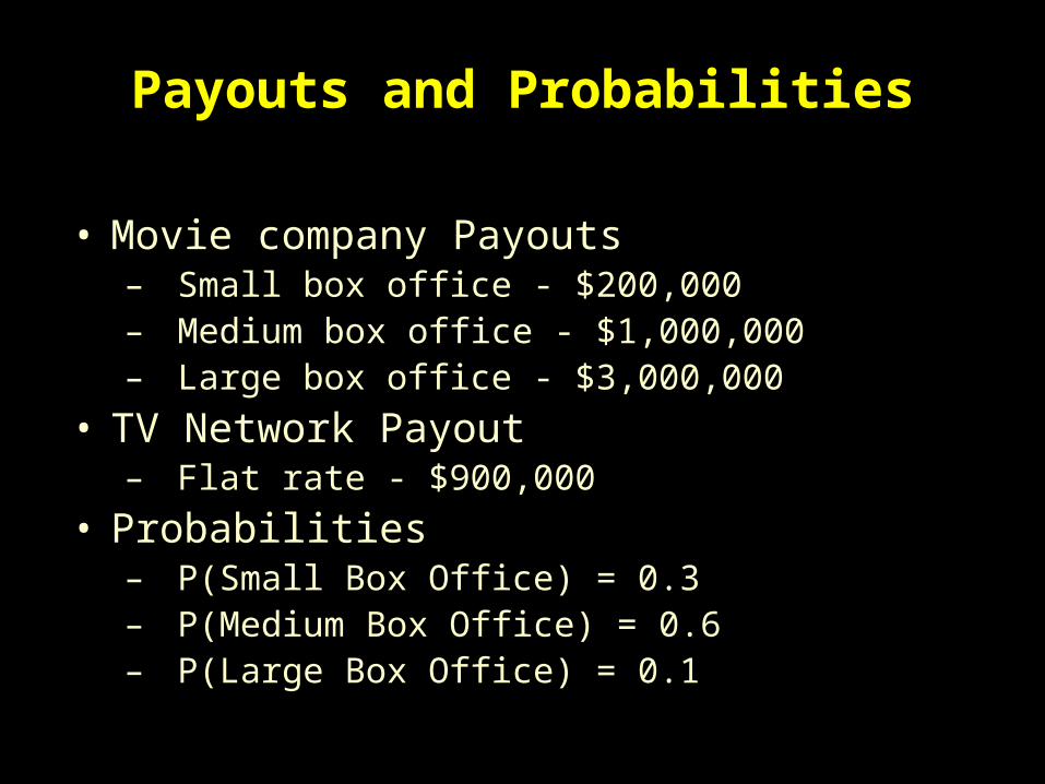
Payouts and Probabilities

• Movie company Payouts– Small box office - $200,000– Medium box office - $1,000,000– Large box office - $3,000,000

• TV Network Payout– Flat rate - $900,000

• Probabilities– P(Small Box Office) = 0.3– P(Medium Box Office) = 0.6– P(Large Box Office) = 0.1

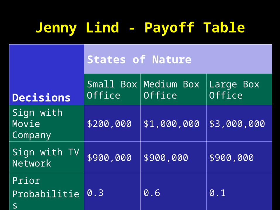
Jenny Lind - Payoff Table

Decisions

States of Nature

Small Box Office

Medium Box Office

Large Box Office

Sign with Movie Company

$200,000 $1,000,000 $3,000,000

Sign with TV Network

$900,000 $900,000 $900,000

Prior

Probabilities0.3 0.6 0.1

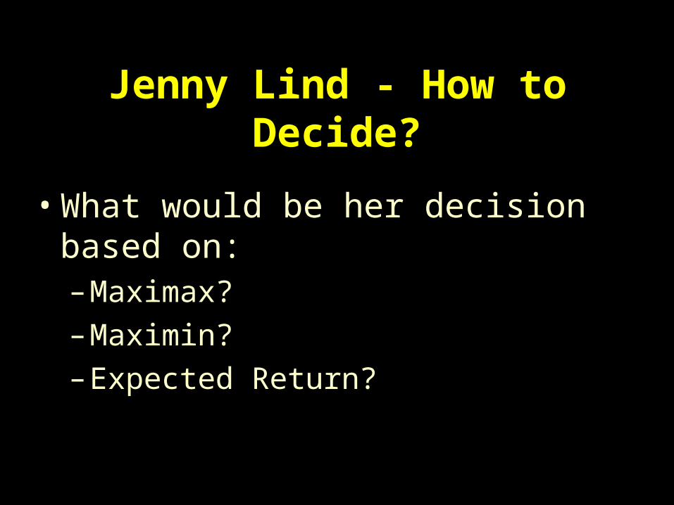
Jenny Lind - How to Decide?

• What would be her decision based on:– Maximax?

– Maximin?

– Expected Return?

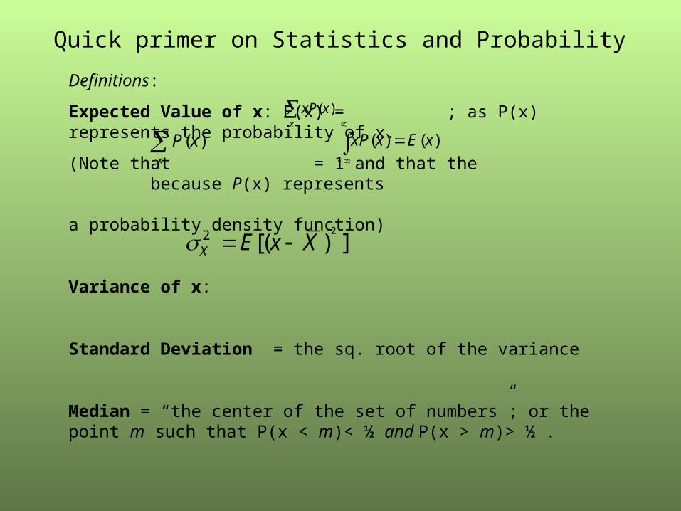
Quick primer on Statistics and Probability

Definitions:

Expected Value of x: E(x) = ; as P(x) represents the probability of x.

(Note that = 1 and that the because P(x) represents

a probability density function)

 

Variance of x:

 

Standard Deviation = the sq. root of the variance

 

Median = “the center of the set of numbers”; or the point m such that P(x < m)< ½ and P(x > m)> ½ .

x

xxP )(

x

xP )(

)()( xExxP

22 [( ) ]X E x X

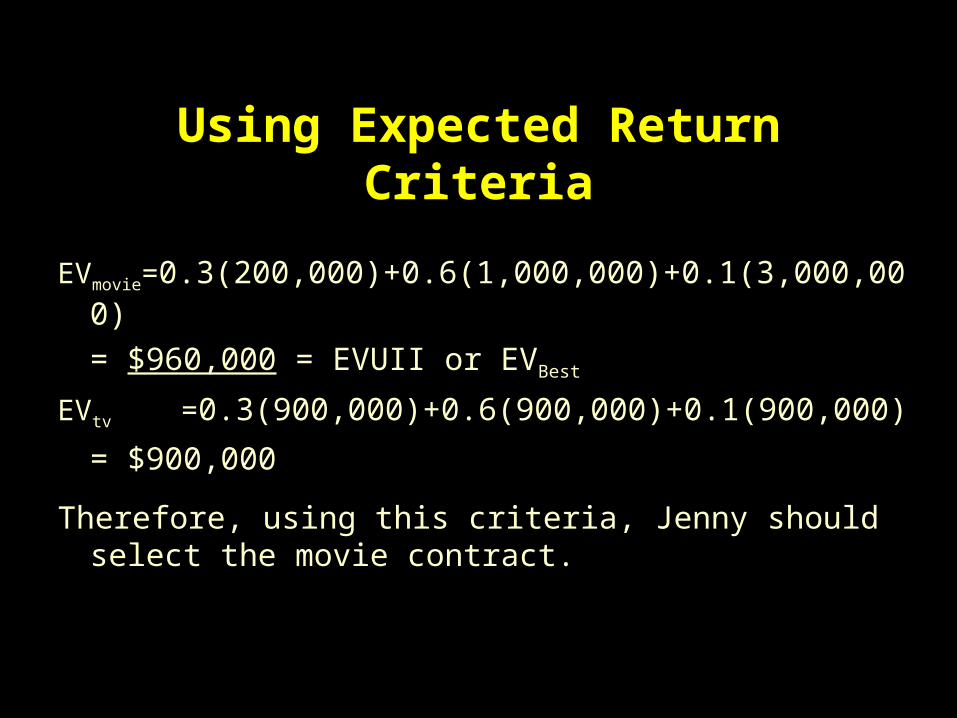
Using Expected Return Criteria

EVmovie=0.3(200,000)+0.6(1,000,000)+0.1(3,000,000)

= $960,000 = EVUII or EVBest

EVtv =0.3(900,000)+0.6(900,000)+0.1(900,000)

= $900,000

Therefore, using this criteria, Jenny should select the movie contract.

Something to Remember

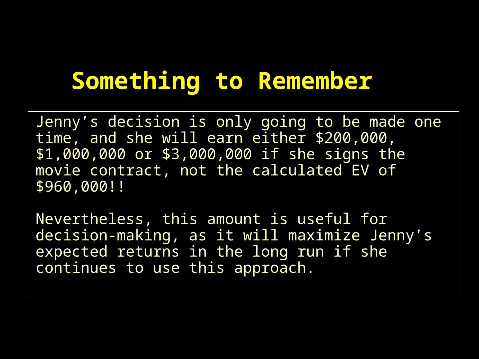
Jenny’s decision is only going to be made one time, and she will earn either $200,000, $1,000,000 or $3,000,000 if she signs the movie contract, not the calculated EV of $960,000!!

Nevertheless, this amount is useful for decision-making, as it will maximize Jenny’s expected returns in the long run if she continues to use this approach.

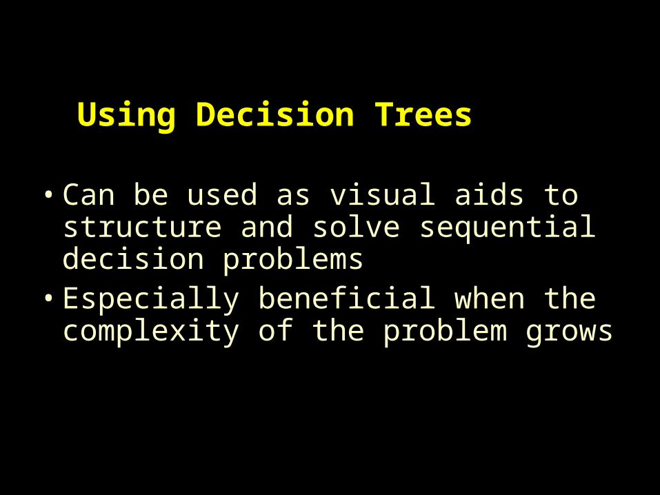
Using Decision Trees

• Can be used as visual aids to structure and solve sequential decision problems

• Especially beneficial when the complexity of the problem grows

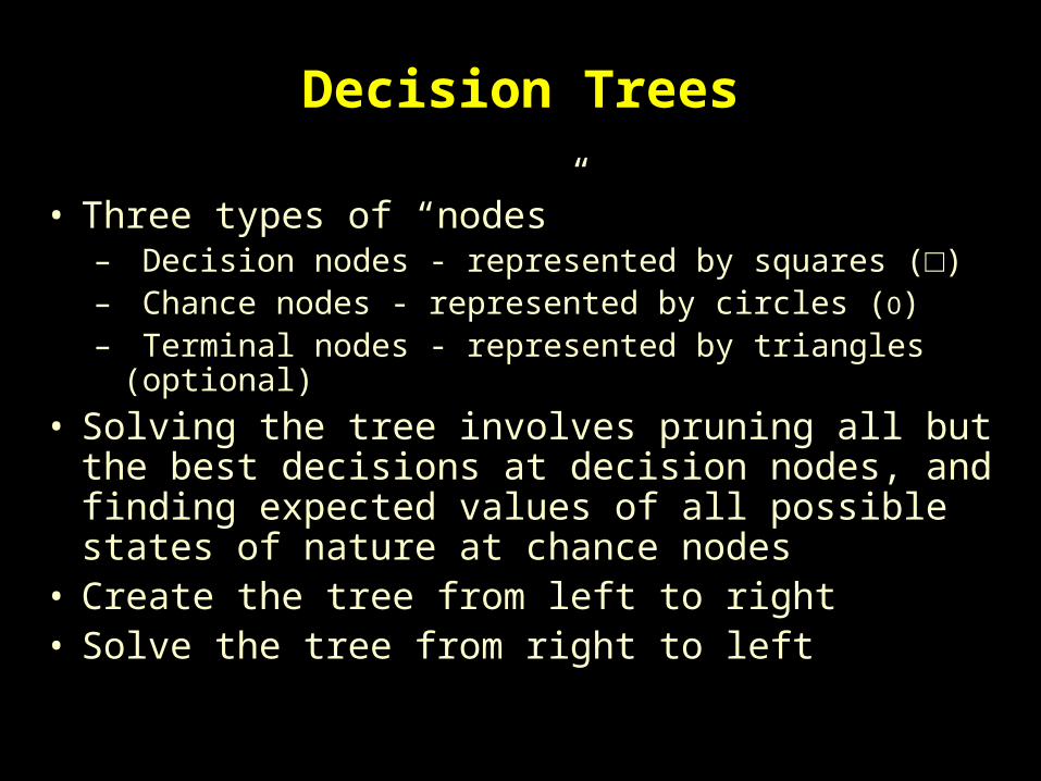
Decision Trees

• Three types of “nodes”– Decision nodes - represented by squares (□)– Chance nodes - represented by circles (Ο)– Terminal nodes - represented by triangles (optional)

• Solving the tree involves pruning all but the best decisions at decision nodes, and finding expected values of all possible states of nature at chance nodes

• Create the tree from left to right • Solve the tree from right to left

Jenny Lind Decision Tree

Small Box Office

Medium Box Office

Large Box Office

Small Box Office

Medium Box Office

Large Box Office

Sign with Movie Co.

Sign with TV Network

$200,000

$1,000,000

$3,000,000

$900,000

$900,000

$900,000

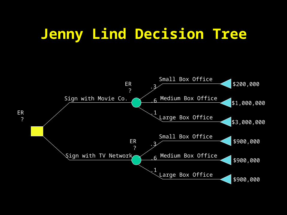
Jenny Lind Decision Tree

Small Box Office

Medium Box Office

Large Box Office

Small Box Office

Medium Box Office

Large Box Office

Sign with Movie Co.

Sign with TV Network

$200,000

$1,000,000

$3,000,000

$900,000

$900,000

$900,000

.3

.6

.1

.3

.6

.1

ER ?

ER ?

ER ?

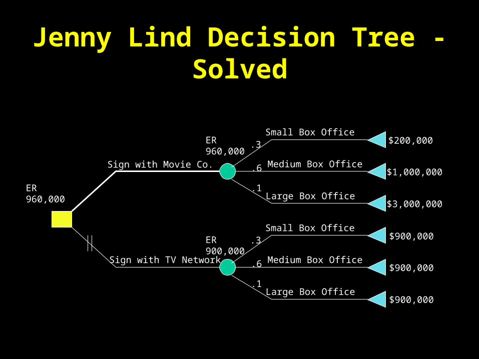
Jenny Lind Decision Tree - Solved

Small Box Office

Medium Box Office

Large Box Office

Small Box Office

Medium Box Office

Large Box Office

Sign with Movie Co.

Sign with TV Network

$200,000

$1,000,000

$3,000,000

$900,000

$900,000

$900,000

.3

.6

.1

.3

.6

.1

ER900,000

ER960,000

ER960,000

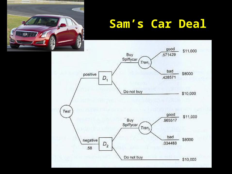
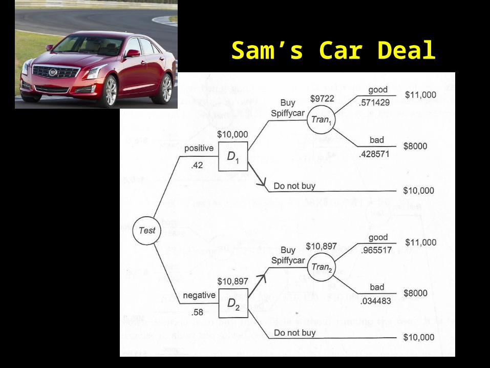
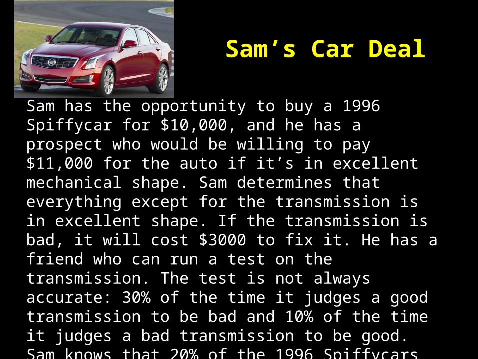
Sam has the opportunity to buy a 1996 Spiffycar for $10,000, and he has a prospect who would be willing to pay $11,000 for the auto if it’s in excellent mechanical shape. Sam determines that everything except for the transmission is in excellent shape. If the transmission is bad, it will cost $3000 to fix it. He has a friend who can run a test on the transmission. The test is not always accurate: 30% of the time it judges a good transmission to be bad and 10% of the time it judges a bad transmission to be good. Sam knows that 20% of the 1996 Spiffycars have bad transmission.

Draw a decision tree for Sam and tell him what he should do.

Sam’s Car Deal

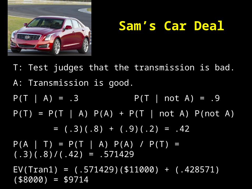
T: Test judges that the transmission is bad.

A: Transmission is good.

P(T | A) = .3 P(T | not A) = .9

P(T) = P(T | A) P(A) + P(T | not A) P(not A)

= (.3)(.8) + (.9)(.2) = .42

P(A | T) = P(T | A) P(A) / P(T) = (.3)(.8)/(.42) = .571429

EV(Tran1) = (.571429)($11000) + (.428571)($8000) = $9714

Similarly, EV(Tran2) = $10897

Sam’s Car Deal

Sam’s Car Deal

Sam’s Car Deal

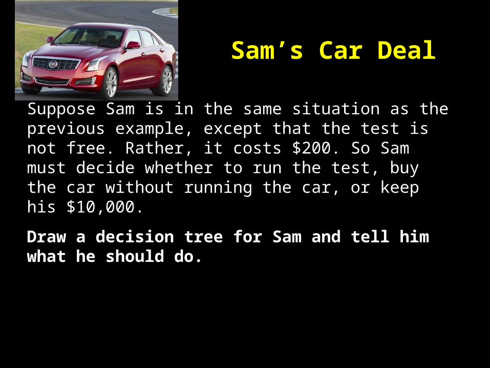
Suppose Sam is in the same situation as the previous example, except that the test is not free. Rather, it costs $200. So Sam must decide whether to run the test, buy the car without running the car, or keep his $10,000.

Draw a decision tree for Sam and tell him what he should do.

Sam’s Car Deal

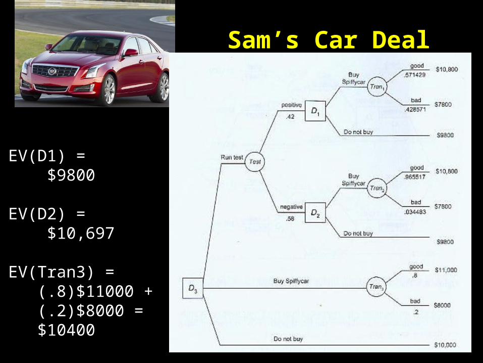
Sam’s Car Deal

EV(D1) = $9800

EV(D2) = $10,697 EV(Tran3) = (.8)$11000 + (.2)$8000 = $10400

Mary’s Factory

Mary is the CEO of a gadget factory.

She is wondering whether or not it is a good idea to expand her factory this year. The cost to expand her factory is $1.5M. If she expands the factory, she expects to receive $6M if economy is good and people continue to buy lots of gadgets, and $2M if economy is bad.

If she does nothing and the economy stays good she expects $3M in revenue; while only $1M if the economy is bad.

She also assumes that there is a 40% chance of a good economy and a 60% chance of a bad economy.

Draw a Decision Tree showing these choices.

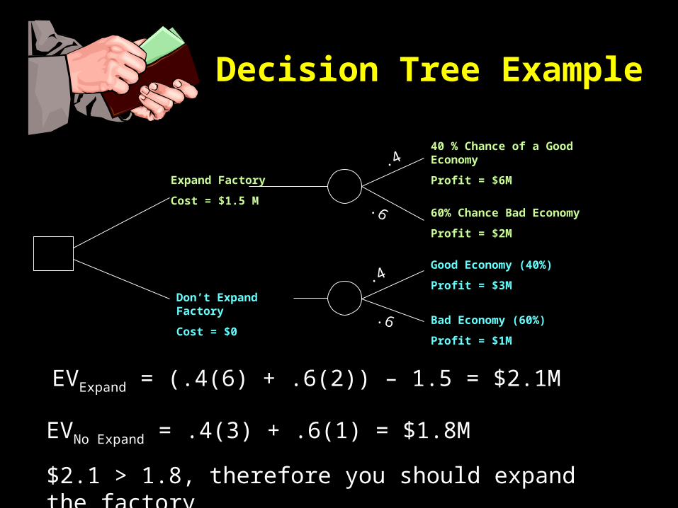
Decision Tree Example

Expand Factory

Cost = $1.5 M

Don’t Expand Factory

Cost = $0

40 % Chance of a Good Economy

Profit = $6M

60% Chance Bad Economy

Profit = $2M

Good Economy (40%)

Profit = $3M

Bad Economy (60%)

Profit = $1M

EVExpand = (.4(6) + .6(2)) – 1.5 = $2.1M

EVNo Expand = .4(3) + .6(1) = $1.8M

$2.1 > 1.8, therefore you should expand the factory

.4

.4

.6

.6

Mary’s Factory – Discounting

Before Mary takes this to the board, she wants to account for the time value of money. The gadget company uses a 10% discount rate (interest). The cost of expanding the factory is paid in year zero but the revenue streams are in year one.

 

Compute the NPV again, this time accounts the time value of money in your analysis. Should she expand the factory?

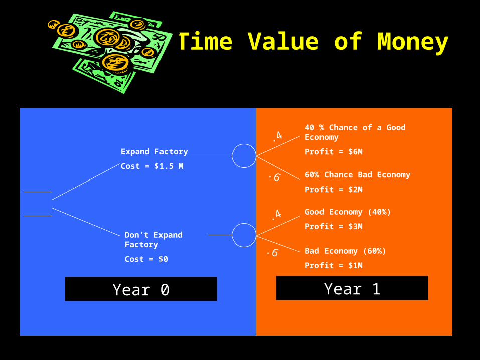
Time Value of Money

Year 0 Year 1

Expand Factory

Cost = $1.5 M

Don’t Expand Factory

Cost = $0

40 % Chance of a Good Economy

Profit = $6M

60% Chance Bad Economy

Profit = $2M

Good Economy (40%)

Profit = $3M

Bad Economy (60%)

Profit = $1M

.4

.4

.6

.6

Time Value of Money

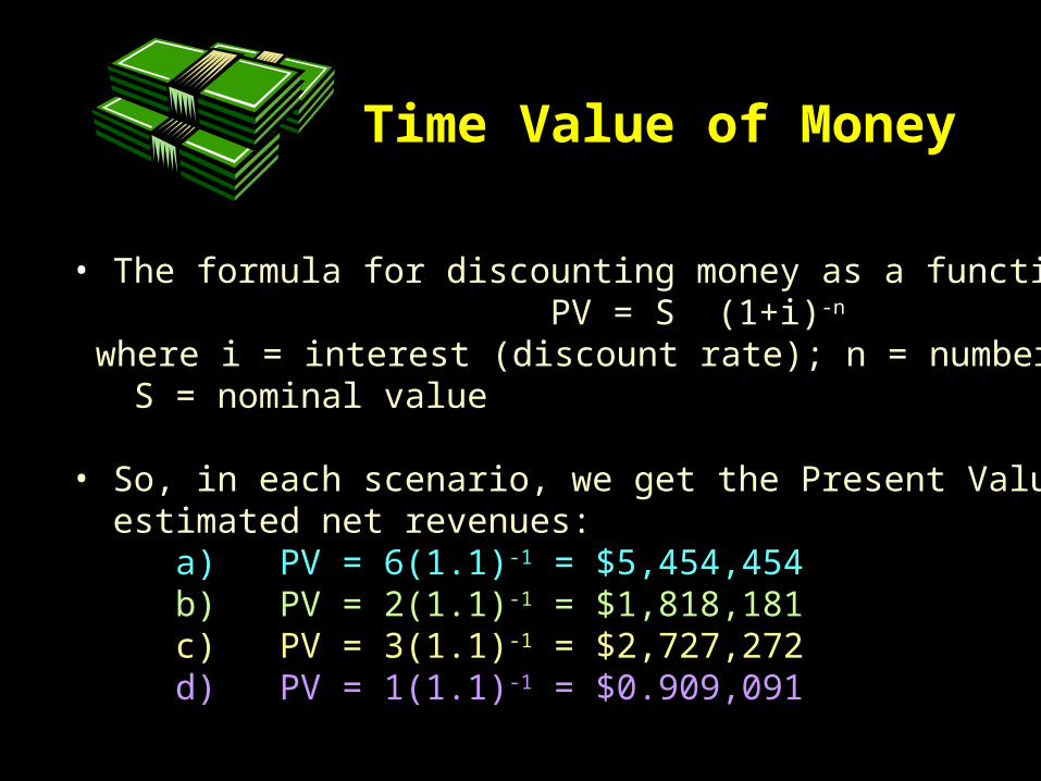
• The formula for discounting money as a function of time is: PV = S (1+i)-n

where i = interest (discount rate); n = number of years; S = nominal value • So, in each scenario, we get the Present Value (PV) of the estimated net revenues:

a) PV = 6(1.1)-1 = $5,454,454b) PV = 2(1.1)-1 = $1,818,181c) PV = 3(1.1)-1 = $2,727,272d) PV = 1(1.1)-1 = $0.909,091

Time Value of Money

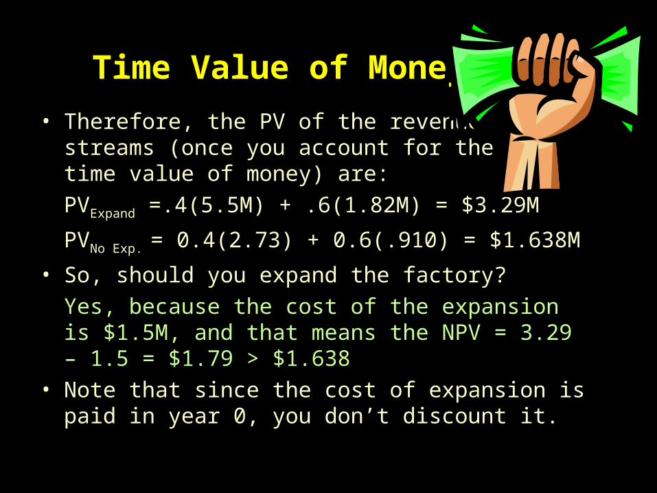
• Therefore, the PV of the revenue streams (once you account for the time value of money) are:

PVExpand =.4(5.5M) + .6(1.82M) = $3.29M

PVNo Exp. = 0.4(2.73) + 0.6(.910) = $1.638M

• So, should you expand the factory?

Yes, because the cost of the expansion is $1.5M, and that means the NPV = 3.29 – 1.5 = $1.79 > $1.638

• Note that since the cost of expansion is paid in year 0, you don’t discount it.

Stephanie’s Hardware Store

Stephanie has a hardware store and she is deciding whether or not to buy Adler’s Hardware store. She can buy it for $400,000; however it would take one year to renovate, implement her computer inventory system, etc.

The next year she expects to earn an additional $600,000 if the economy is good and only $200,000 if the economy is bad. She estimates a 65% probability of a good economy and a 35% probability of a bad economy. If she doesn’t buy Adler’s she knows she will get $0 additional profits.

Taking the time value of money into account, find the NPV of the project with a discount rate of 10%

Answer to Stephanie’s Problem

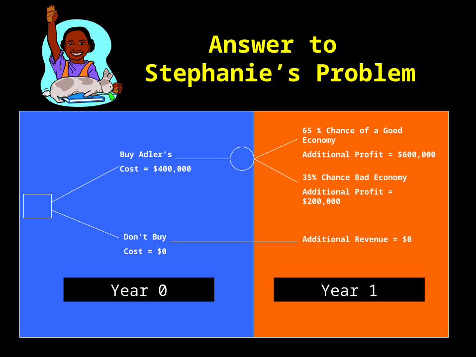
Year 0 Year 1

Buy Adler’s

Cost = $400,000

Don’t Buy

Cost = $0

65 % Chance of a Good Economy

Additional Profit = $600,000

35% Chance Bad Economy

Additional Profit = $200,000

Additional Revenue = $0

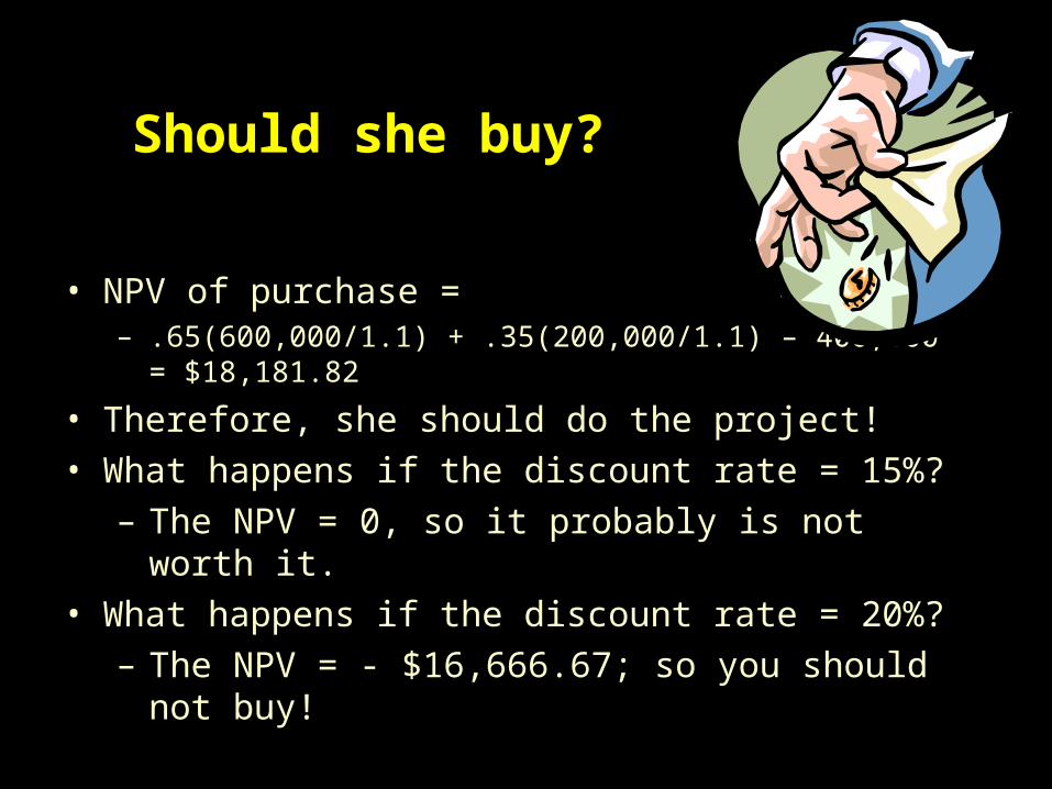
Should she buy?

• NPV of purchase =– .65(600,000/1.1) + .35(200,000/1.1) – 400,000

= $18,181.82

• Therefore, she should do the project!• What happens if the discount rate = 15%?

– The NPV = 0, so it probably is not worth it.• What happens if the discount rate = 20%?

– The NPV = - $16,666.67; so you should not buy!

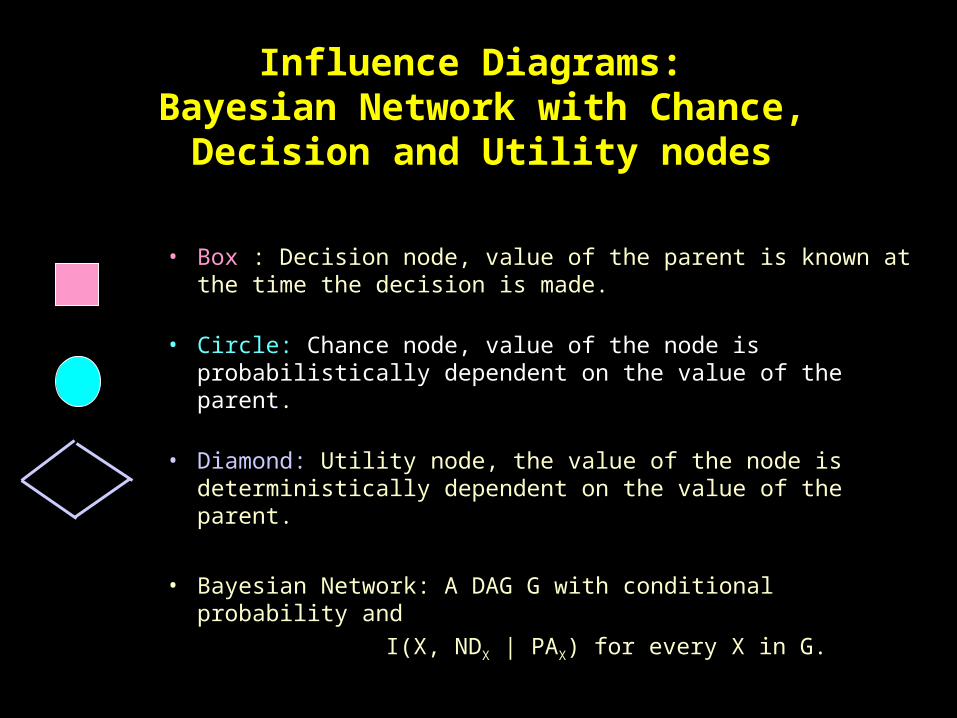
Influence Diagrams: Bayesian Network with Chance, Decision

and Utility nodes

• Box : Decision node, value of the parent is known at the time the decision is made.

• Circle: Chance node, value of the node is probabilistically dependent on the value of the parent.

• Diamond: Utility node, the value of the node is deterministically dependent on the value of the parent.

• Bayesian Network: A DAG G with conditional probability and

I(X, NDX | PAX) for every X in G.

Sam has the opportunity to buy a 1996 Spiffycar for $10,000, and he has a prospect who would be willing to pay $11,000 for the auto if it’s in excellent mechanical shape. Sam determines that everything except for the transmission is in excellent shape. If the transmission is bad, it will cost $3000 to fix it. He has a friend who can run a test on the transmission. The test is not always accurate: 30% of the time it judges a good transmission to be bad and 10% of the time it judges a bad transmission to be good. Sam knows that 20% of the 1996 Spiffycars have bad transmission.

Draw a decision tree for Sam and tell him what he should do.

Sam’s Car Deal

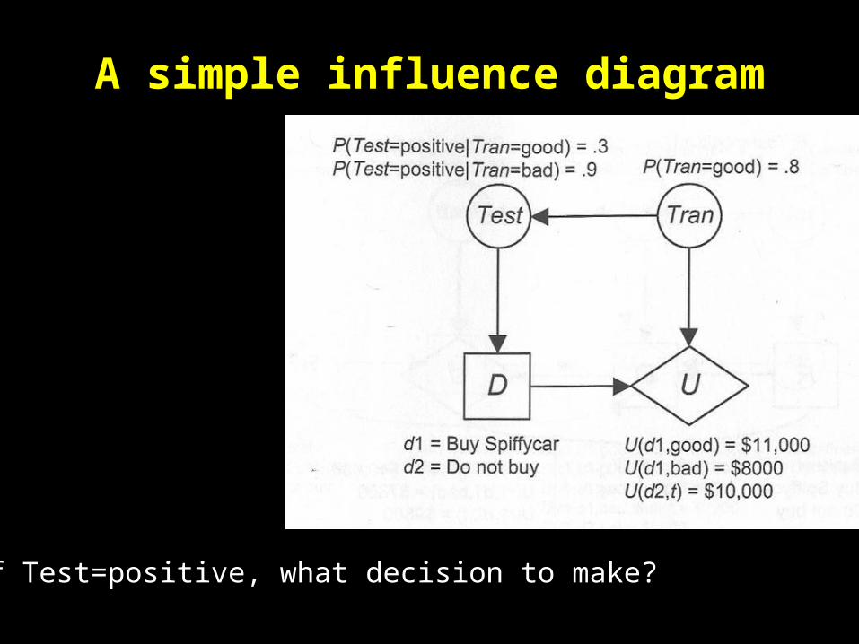
A simple influence diagram

If Test=positive, what decision to make?

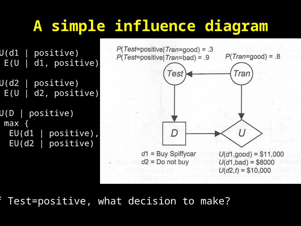
A simple influence diagram

If Test=positive, what decision to make?

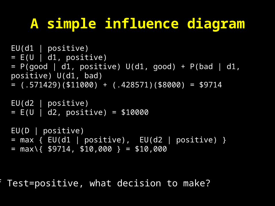
EU(d1 | positive) = E(U | d1, positive)

EU(d2 | positive) = E(U | d2, positive)

EU(D | positive) = max { EU(d1 | positive), EU(d2 | positive) }

A simple influence diagram

If Test=positive, what decision to make?

EU(d1 | positive) = E(U | d1, positive) = P(good | d1, positive) U(d1, good) + P(bad | d1, positive) U(d1, bad) = (.571429)($11000) + (.428571)($8000) = $9714 EU(d2 | positive) = E(U | d2, positive) = $10000

EU(D | positive) = max { EU(d1 | positive), EU(d2 | positive) }= max\{ $9714, $10,000 } = $10,000

T: Test judges that the transmission is bad.

A: Transmission is good.

P(T | A) = .3 P(T | not A) = .9

P(T) = P(T | A) P(A) + P(T | not A) P(not A)

= (.3)(.8) + (.9)(.2) = .42

P(A | T) = P(T | A) P(A) / P(T) = (.3)(.8)/(.42) = .571429

EV(Tran1) = (.571429)($11000) + (.428571)($8000) = $9714

Similarly, EV(Tran2) = $10897

Sam’s Car Deal

Suppose Sam is in the same situation as the previous example, except that the test is not free. Rather, it costs $200. So Sam must decide whether to run the test, buy the car without running the car, or keep his $10,000.

Draw a decision tree for Sam and tell him what he should do.

Sam’s Car Deal

A simple influence diagram

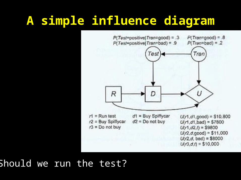
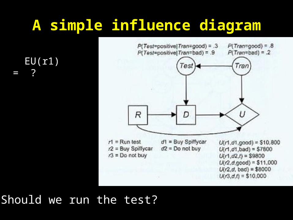
Should we run the test?

A simple influence diagram

Should we run the test?

EU(r1) = ?

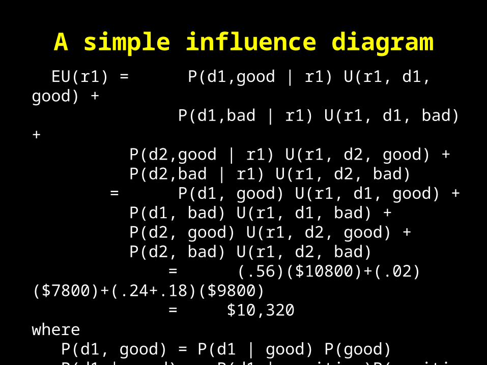
A simple influence diagram EU(r1) = P(d1,good | r1) U(r1, d1, good) + P(d1,bad | r1) U(r1, d1, bad) + P(d2,good | r1) U(r1, d2, good) + P(d2,bad | r1) U(r1, d2, bad)

= P(d1, good) U(r1, d1, good) + P(d1, bad) U(r1, d1, bad) + P(d2, good) U(r1, d2, good) + P(d2, bad) U(r1, d2, bad) = (.56)($10800)+(.02)($7800)+(.24+.18)($9800) = $10,320where P(d1, good) = P(d1 | good) P(good) P(d1 | good) = P(d1 | positive)P(positive | good) + P(d1 | negative)P(negative | good) = P(negative | good) = .7

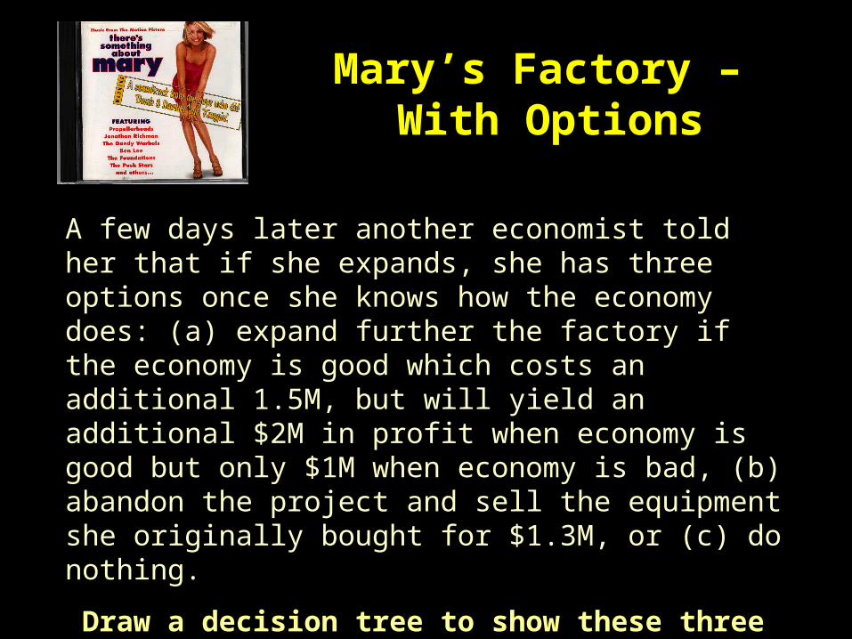
Mary’s Factory – With Options

A few days later another economist told her that if she expands, she has three options once she knows how the economy does: (a) expand further the factory if the economy is good which costs an additional 1.5M, but will yield an additional $2M in profit when economy is good but only $1M when economy is bad, (b) abandon the project and sell the equipment she originally bought for $1.3M, or (c) do nothing.

Draw a decision tree to show these three options for each possible outcome, and compute the EV for the expansion.

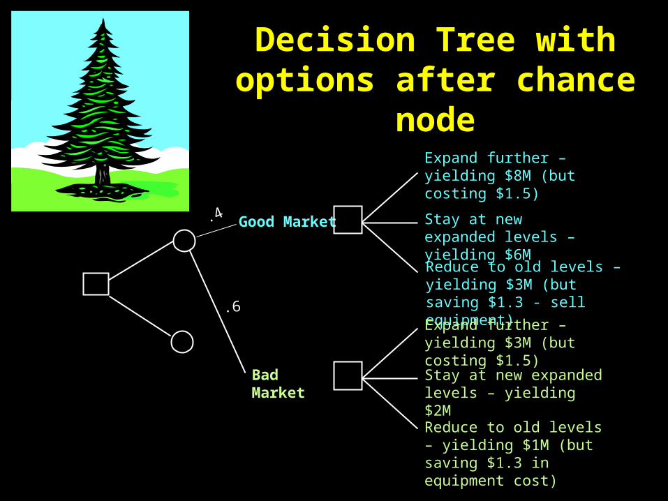
Decision Tree with options after chance node

Good Market

Bad Market

Expand further – yielding $8M (but costing $1.5)

Stay at new expanded levels – yielding $6M

Reduce to old levels – yielding $3M (but saving $1.3 - sell equipment)

Expand further – yielding $3M (but costing $1.5)

Stay at new expanded levels – yielding $2M

Reduce to old levels – yielding $1M (but saving $1.3 in equipment cost)

.4

.6

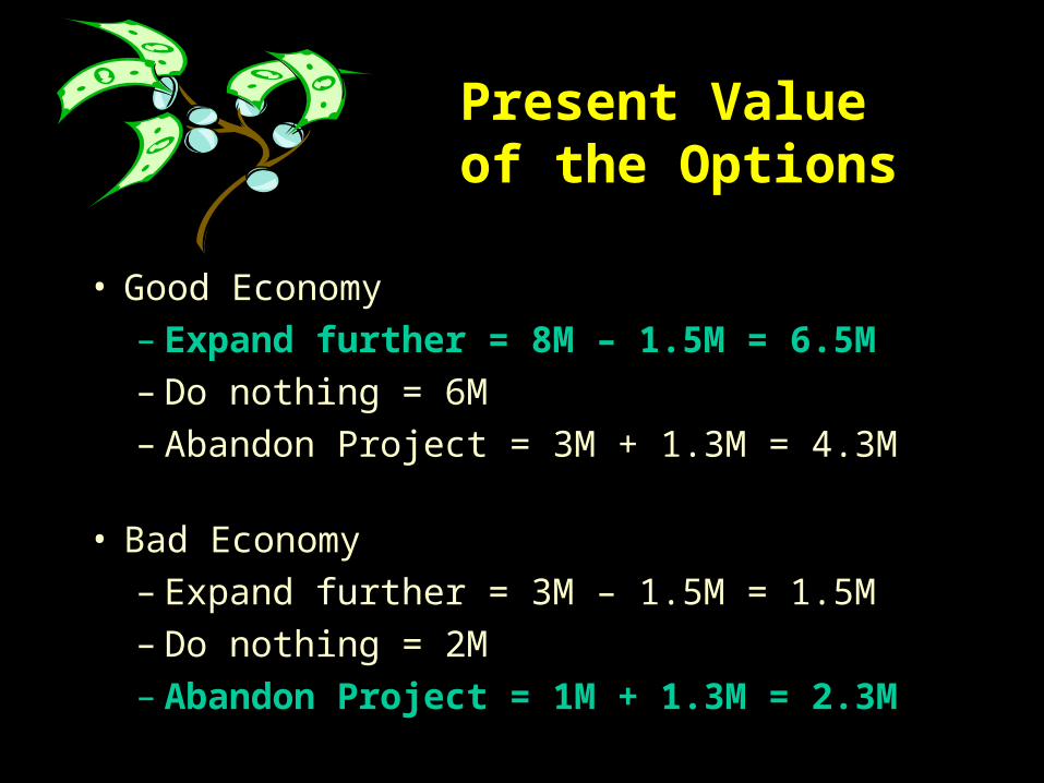
Present Value of the Options

• Good Economy– Expand further = 8M – 1.5M = 6.5M – Do nothing = 6M – Abandon Project = 3M + 1.3M = 4.3M

• Bad Economy– Expand further = 3M – 1.5M = 1.5M– Do nothing = 2M – Abandon Project = 1M + 1.3M = 2.3M

NPV of the Project

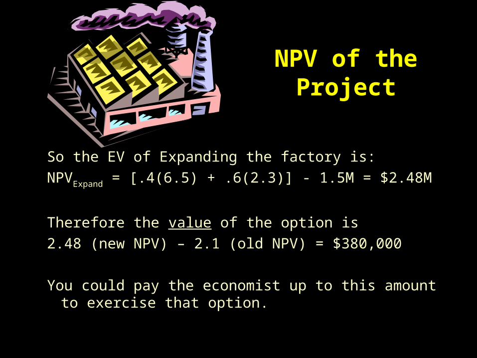
So the EV of Expanding the factory is:

NPVExpand = [.4(6.5) + .6(2.3)] - 1.5M = $2.48M

Therefore the value of the option is

2.48 (new NPV) – 2.1 (old NPV) = $380,000

You could pay the economist up to this amount to exercise that option.