Embed Size (px)
Citation preview
1:: Algorithms
Sorting and bin packing.
4:: Route inspection
Find the shortest route which travels along all roads
2:: Graphs and networks
What is a graph and how they represent things.
5:: The Travelling Salesman
Find the shortest route which visits all places.
3:: Algorithms on graphs
What algorithms do I need to be able to apply?
6:: Linear Programming
How to find an optimal solution graphically
7:: The simplex algorithm
How to find an optimal solution algebraically.
8:: Critical path analysis
How to plan a project.
Decision 1 Overview

Linear Programming
Linear Programming is an optimisation technique. It involves making the most, or the least, of something when subjected to some (linear) constraints.
In this chapter we will deal with constrained problems in two independent variables, but the same process can be applied to higher dimensional problems.
Rather than try and give you examples of when linear programming is useful, try to think of any situation where you are trying to make something and you don’t have constraints?
https://www.geogebra.org/m/twb5mtec

Formulating the problem
Mr Blackett is thinking of taking a break from teaching Decision Maths and setting up a business making and selling Mobius Strips and Klein Bottles hewn from solid gold. He invests in a 3-D CNC milling machine and sets about defining the constraints as a linear programming problem.
• Each Klein bottle takes 2 hours to mill and 3 hours to polish.• Each Mobius strip takes 3 hours to mill and 1 hour to polish.
The milling machine can run for 80 hours per week. Mr Blackett can polish for 60 hours a week.
He believes he can make £2,000 profit on every Klein bottle and £1,000 profit on every Mobius Strip. He wishes to maximise his profit!
First define the decision variables.
Next state the objective.
Then identify the constraints.
Let 𝑥 be the number of Klein bottles and 𝑦 be the number of Mobius strips produced in a week.
Maximise 𝑃 = 2000𝑥 + 1000𝑦
Milling, 2𝑥 + 3𝑦 ≤ 80Polishing, 3𝑥 + 𝑦 ≤ 60Non Negativity, 𝑥, 𝑦 ≥ 0
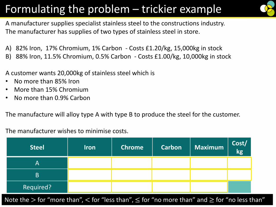
Formulating the problem – trickier exampleA manufacturer supplies specialist stainless steel to the constructions industry.The manufacturer has supplies of two types of stainless steel in store.
A) 82% Iron, 17% Chromium, 1% Carbon - Costs £1.20/kg, 15,000kg in stockB) 88% Iron, 11.5% Chromium, 0.5% Carbon - Costs £1.00/kg, 10,000kg in stock
A customer wants 20,000kg of stainless steel which is • No more than 85% Iron• More than 15% Chromium• No more than 0.9% Carbon
The manufacture will alloy type A with type B to produce the steel for the customer.
The manufacturer wishes to minimise costs.
Steel Iron Chrome Carbon MaximumCost/
kg
A 82% 17% 1% 15,000 £1.20
B 88% 11.5% 0.5% 10,000 £1
Required? ≤ 85% > 15% ≤ 0.9% 20,000
Note the > for “more than”, < for “less than”, ≤ for “no more than” and ≥ for “no less than”

Steel Iron Chrome Carbon Maximum Cost/kg
A (𝑥) 82% 17% 1% 15,000 £1.20
B (𝑦) 88% 11.5% 0.5% 10,000 £1
Required? ≤ 85% > 15% ≤ 0.9% 20,000
Formulating the problem – trickier example ctd.
Define the decision variables
Let 𝑥 be the number of kg of type A used.Let 𝑦 be the number of kg of type B used.
State the objective
Minimise 𝐶 = 1.2𝑥 + 𝑦
State (and simplify) the constraints0.82𝑥 + 0.88𝑦 ≤ 0.85 𝑥 + 𝑦
0.03𝑦 ≤ 0.03𝑥𝑦 ≤ 𝑥
State (and simplify) the constraints (ctd.)0.17𝑥 + 0.115𝑦 > 0.15 𝑥 + 𝑦
0.02𝑥 > 0.035𝑦𝑥 > 1.75𝑦
0.01𝑥 + 0.005𝑦 ≤ 0.009 𝑥 + 𝑦1
4𝑥 ≤ 𝑦
A customer wants 20,000kg of stainless steel which is • No more than 85% Iron• More than 15%
Chromium• No more than 0.9%
Carbon
𝑥 + 𝑦 ≥ 20,000𝑥 ≤ 15,000𝑦 ≤ 10,000
𝑥, 𝑦 ≥ 0
Note we define this constraint as ≥ even though it is obvious that the optimal solution will be =, this lets us define a valid solution region which we may use for later adjustments to the problem.

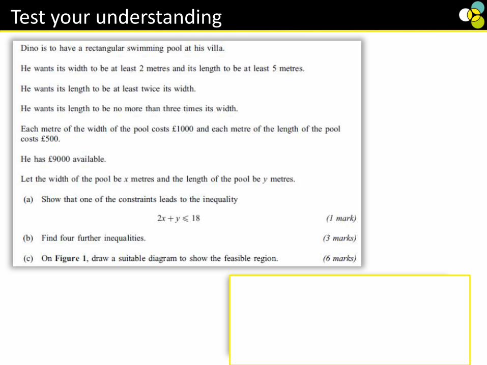
Test your understanding

Pearson Decision 1, Page 143
Exercise 6A

Graphical Methods
The region of a graph that satisfies all the constraints of a linear programming problem is called the feasible region.
The convention for linear programming problems is to leave the feasible region (which satisfies all inequalities) unshaded. Graphing software (such as Desmos), always shade the region which satisfies the inequality, so be careful if using graphing software to check your answers.
Height of vase (cm)
Hei
ght
of
arra
nge
men
t (c
m)
It is a well known rule of flower arranging that the overall height of the arrangement should be between 1.5 and twice the height of the vase. We can visualise this on the plot on the right, with the white region representing the feasible region for the vase/arrangement combinations.

Graphing the problemRecall that Mr Blackett is thinking of branching out, earlier we formulated his problem as the following inequalities.
Let 𝑥 be the number of Klein bottlesLet 𝑦 be the number of Mobius strips produced in a week.
Maximise 𝑃 = 2000𝑥 + 1000𝑦
Milling, 2𝑥 + 3𝑦 ≤ 80Polishing, 3𝑥 + 𝑦 ≤ 60Non Negativity, 𝑥, 𝑦 ≥ 0
𝑥, 𝑦 ≥ 0
Put a solid line on the 𝑥 and 𝑦 axis and shade the negative regions.
3𝑥 + 𝑦 ≤ 60First let 𝑥 = 0 ∴ 𝑦 = 60Then let 𝑦 = 0 ∴ 𝑥 = 20
Plot with a solid line as it is ≤
2𝑥 + 3𝑦 ≤ 80
First let 𝑥 = 0 ∴ 𝑦 = 262
3
Then let 𝑦 = 0 ∴ 𝑥 = 40
Plot with a solid line as it is ≤Shade the unwanted region
Clicky graph

Test your understandingAgain recall that we had a customer wanting to buy 20,000kg of stainless steel. We formulated the problem with the following constraints.
Let 𝑥 be the number of kg of type A used.Let 𝑦 be the number of kg of type B used.
𝑦 ≤ 𝑥𝑥 > 1.75𝑦1
4𝑥 ≤ 𝑦
𝑥 ≤ 15,000𝑦 ≤ 10,000𝑥 + 𝑦 ≥ 20,000𝑥, 𝑦 ≥ 0
𝑥, 𝑦 ≥ 0
Put a solid line on the 𝑥 and 𝑦 axis and shade the negative regions.
𝑥 + 𝑦 ≥ 20,000
When 𝑥 = 0, 𝑦 = 20,000When y = 0, 𝑥 = 20,000Plot this with a solid line and shade below it.
𝑥 ≤ 15,000𝑦 ≤ 10,000
Plot these two lines, and shade above them.
1
4𝑥 ≤ 𝑦
Plot the line 𝑦 =1
4𝑥
Check a point either side of it to determine which side to shade.
𝑥 > 1.75𝑦Plot the line 𝑥 = 1.75𝑦Pick a point, say 𝑥 = 20,000 𝑦 = 11 429 to help plot. Plot with dotted line, as it is >Check a point either side of it to determine which side to shade.
𝑦 ≤ 𝑥
Plot the line 𝑦 = 𝑥, with a solid line.
Check a point either side of it to determine which side to shade.
Clicky graph
Test your understanding
Clicky graph
Pearson Decision 1, Page 147
Exercise 6B

Finding a minimum point – sliding ruler methodRecall that we had a customer wanting to buy 20,000kg of stainless steel, earlier we formulated his problem as inequalities, and graphed them as shown below.
This graph shows us the feasible region – what values of type A and type B that the customer would accept in the mix.
It doesn’t tell us which of these points is optimal, that is, which is going to minimise cost.
https://www.desmos.com/calculator/vnfvgt3lcr

Finding a minimum point – sliding ruler method
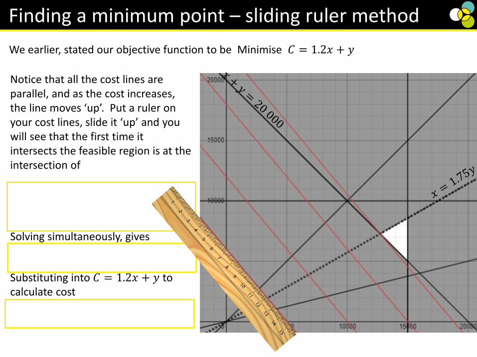
We earlier, stated our objective function to be Minimise 𝐶 = 1.2𝑥 + 𝑦
The objective function is not one line, but an infinite family of parallel lines.
We can plot the objective function if we assume a value of C.
Lets look at a few examples
𝐶 = 12 00012 000 = 1.2𝑥 + 𝑦When 𝑥 = 0, 𝑦 = 12 000When 𝑦 = 0, 𝑥 = 10 000
𝐶 = 18 00018 000 = 1.2𝑥 + 𝑦When 𝑥 = 0, 𝑦 = 18 000When 𝑦 = 0, 𝑥 = 15 000
𝐶 = 6 0006 000 = 1.2𝑥 + 𝑦When 𝑥 = 0, 𝑦 = 6 000When 𝑦 = 0, 𝑥 = 5 000
Finding a minimum point – sliding ruler method
We earlier, stated our objective function to be Minimise 𝐶 = 1.2𝑥 + 𝑦
Notice that all the cost lines are parallel, and as the cost increases, the line moves ‘up’. Put a ruler on your cost lines, slide it ‘up’ and you will see that the first time it intersects the feasible region is at the intersection of
𝑥 = 1.75𝑦and
𝑥 + 𝑦 = 20 000Solving simultaneously, gives
𝑥 =140000
11, 𝑦 =
80000
11Substituting into 𝐶 = 1.2𝑥 + 𝑦 to calculate cost
Gives 𝐶 =248000
11≈ £22545

Maximum Profit 𝑃 = 6.75 × 2 + 4.5 × 5 = 36
Finding a maximum point - sliding ruler method
For a maximum point, look for the last point covered by an objective line as it leaves the feasible region. For a minimum point, look for the first point covered by an objective line as it enters the feasible region.
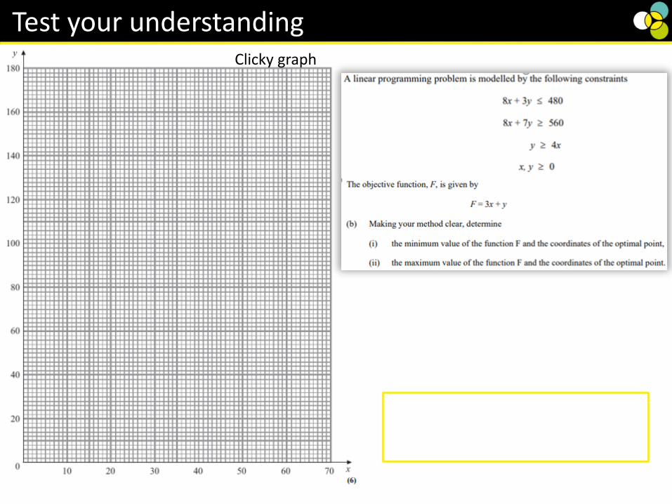
A linear programming problem is formulated such that,
𝑦 ≤2
3𝑥,
𝑥 ≤ 8𝑦 ≤ −2𝑥 + 18𝑦 ≥ −0.5𝑥 + 5
Show the feasible region on the axis opposite.
The objective function is to maximise 𝑃 = 2𝑥 + 5𝑦
By plotting a profit line for a value of P, then sliding the ruler, find the coordinates of the point of maximum profit and calculate 𝑃 at this point.
https://www.desmos.com/calculator/qbkbkcphh6
Clicky graph
Test your understandingClicky graph

Vertex testing method
To find an optimal point using the vertex testing method:1) Find the coordinates of each vertex of the feasible region.2) Evaluate the objective function at each of these points.3) Select the vertex that gives the optimal value of the objective function..
A feasible region is defined by the following inequalities
2𝑥 + 4𝑦 ≥ 303𝑥 + 𝑦 ≥ 25𝑥 + 𝑦 ≥ 13𝑦 ≥ 1𝑥 ≥ 0
The objective function is to minimise
𝐶 = 140𝑥 + 170𝑦
Vertex 𝒙 𝒚 Value of 𝑪 = 𝟏𝟒𝟎𝒙 + 𝟏𝟕𝟎𝒚
A 0 25 4250
B 6 7 2030
C 11 2 1880
D 13 1 1990
Vertex 𝒙 𝒚 Value of 𝑪 = 𝟏𝟒𝟎𝒙 + 𝟏𝟕𝟎𝒚
A
B
C
D
Sketch the graph to identify the feasible regionthen solve the related simultaneous equations to find the coordinates of each vertex.
Hence the vertex which minimises the objective function is C, with a cost of 1880.
https://www.desmos.com/calculator/o7hauownx9

Test your understanding
The feasible region for a linear programming problem is defined by the following inequalities.
𝑦 ≥ −5𝑥 + 13𝑦 ≥ −𝑥 + 4𝑦 ≥ 1𝑦 ≤ 10𝑥 ≤ 3
The objective function is to minimise 𝐶 =13𝑥 + 14𝑦
By the vertex testing method determine the minimum feasible value of C.
𝑥=4
𝑦 = 10
𝑦 = 1Vertex 𝒙 𝒚 𝑪 = 𝟏𝟑𝒙 + 𝟏𝟒𝒚
A 0.6 10 147.8
B 3 10 179
C 3 1 53
D 2.25 1.75 53.75
A B
C
D
Therefore the min. value of 𝐶 = 53at 3,1
Vertex 𝒙 𝒚 𝑪 = 𝟏𝟑𝒙 + 𝟏𝟒𝒚
A
B
C
D

Pearson Decision 1, Page 158
Exercise 6C
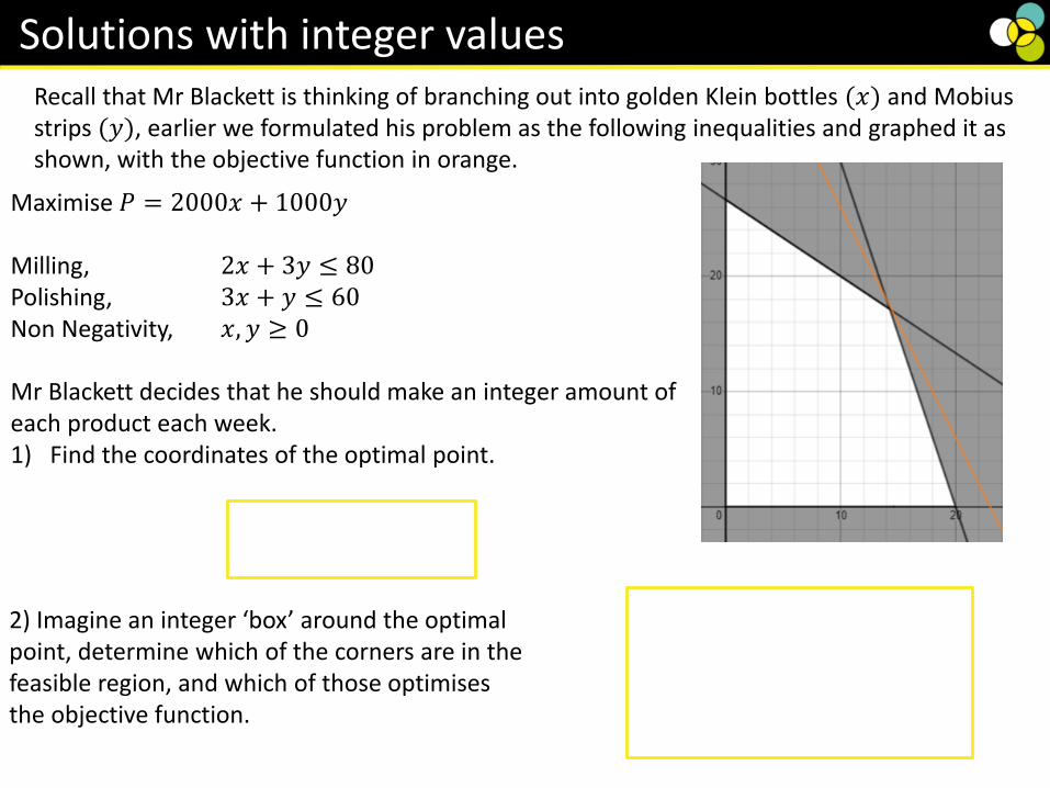
Solutions with integer valuesRecall that Mr Blackett is thinking of branching out into golden Klein bottles (𝑥) and Mobius strips (𝑦), earlier we formulated his problem as the following inequalities and graphed it as shown, with the objective function in orange.
Maximise 𝑃 = 2000𝑥 + 1000𝑦
Milling, 2𝑥 + 3𝑦 ≤ 80Polishing, 3𝑥 + 𝑦 ≤ 60Non Negativity, 𝑥, 𝑦 ≥ 0
Mr Blackett decides that he should make an integer amount of each product each week.1) Find the coordinates of the optimal point.
141
7, 17
1
7
14, 17 15, 17
15, 1814, 182) Imagine an integer ‘box’ around the optimal point, determine which of the corners are in the feasible region, and which of those optimises the objective function.
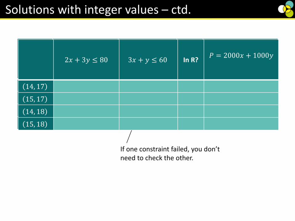
2𝑥 + 3𝑦 ≤ 80 3𝑥 + 𝑦 ≤ 60 In R?𝑃 = 2000𝑥 + 1000𝑦
14, 17 79 ≤ 80 59 ≤ 60 Yes £45,000
15, 17 81 ≰ 80 - No
14, 18 82 ≰ 80 - No
15, 18 84 ≰ 80 - No
Solutions with integer values – ctd.
If one constraint failed, you don’t need to check the other.
2𝑥 + 3𝑦 ≤ 80 3𝑥 + 𝑦 ≤ 60 In R?𝑃 = 2000𝑥 + 1000𝑦
14, 17
15, 17
14, 18
15, 18

Pearson Decision 1, Page 165
Exercise 6D


![Ranking Decision making units using Fuzzy Multi-Objective ......Multi-objective Linear Programming (MOLP) Veeramani et al. [23] Multi-objective Linear Programming (MOLP) Problems is](https://img.pdfslide.us/doc/110x75/610e91b630eca77d674f86aa/ranking-decision-making-units-using-fuzzy-multi-objective-multi-objective.jpg)