Embed Size (px)
Citation preview

University of Central Florida University of Central Florida
STARS STARS
Electronic Theses and Dissertations, 2004-2019
2014
Decentralized Power Management and Transient Control in Hybrid Decentralized Power Management and Transient Control in Hybrid
Fuel Cell Ultra-Capacitor System Fuel Cell Ultra-Capacitor System
Seyed Omid Madani University of Central Florida
Part of the Mechanical Engineering Commons
Find similar works at: https://stars.library.ucf.edu/etd
University of Central Florida Libraries http://library.ucf.edu
This Doctoral Dissertation (Open Access) is brought to you for free and open access by STARS. It has been accepted
for inclusion in Electronic Theses and Dissertations, 2004-2019 by an authorized administrator of STARS. For more
information, please contact [email protected].
STARS Citation STARS Citation Madani, Seyed Omid, "Decentralized Power Management and Transient Control in Hybrid Fuel Cell Ultra-Capacitor System" (2014). Electronic Theses and Dissertations, 2004-2019. 4596. https://stars.library.ucf.edu/etd/4596

Decentralized Power Management and Transient Control in
Hybrid Fuel Cell Ultra-Capacitor System
by
Omid Madani
B.S. Mechanical Engineering, Sharif University of Technology, 2009M.S. Mechanical Engineering, University of Central Florida, 2011
A dissertation submitted in partial fulfillment of the requirementsfor the degree of Doctor of Philosophy
in the Department of Mechanical and Aerospace Engineeringin the College of Engineering and Computer Science
at the University of Central FloridaOrlando, Florida
Fall Term2014
Major Professor: Tuhin Das

© 2014 Omid Madani
ii

ABSTRACT
Solid Oxide Fuel Cells (SOFCs) are considered suitable for alternative energy solutions
due to advantages such as high efficiency, fuel flexibility, tolerance to impurities, and potential
for combined cycle operations. One of the main operating constraints of SOFCs is fuel
starvation, which can occur under fluctuating power demands. It leads to voltage loss and
detrimental effects on cell integrity and longevity. In addition, reformer based SOFCs require
sufficient steam for fuel reforming to avoid carbon deposition and catalyst degradation.
Steam to carbon ratio (STCR) is an index indicating availability of the steam in the reformer.
This work takes a holistic approach to address the aforementioned concerns in SOFCs, in an
attempt to enhance applicability and adaptability of such systems. To this end, we revisit
prior investigation on the invariant properties of SOFC systems, that led to prediction of
fuel utilization U and STCR in the absence of intrusive and expensive sensing. This work
provides further insight into the reasons behind certain SOFC variables being invariant with
respect to operating conditions. The work extends the idea of invariant properties to different
fuel and reformer types.
In SOFCs, transient control is essential for U , especially if the fuel cell is to be oper-
ated in a dynamic load-following mode at high fuel utilization. In this research, we formulate
a generalized abstraction of this transient control problem. We show that a multi-variable
iii

systems approach can be adopted to address this issue in both time and frequency domains,
which leads to input shaping. Simulations show the effectiveness of the approach through
good disturbance rejection. The work further integrates the aforementioned transient con-
trol research with system level control design for SOFC systems hybridized with storage
elements. As opposed to earlier works where centralized robust controllers were of interest,
here, separate controllers for the fuel cell and storage have been the primary emphasis. Thus,
the proposed approach acts as a bridge between existing centralized controls for single fuel
cells to decentralized control for power networks consisting of multiple elements. As a first
attempt, decentralized control is demonstrated in a SOFC ultra-capacitor hybrid system.
The challenge of this approach lies in the absence of direct and explicit communication be-
tween individual controllers. The controllers are designed based on a simple, yet effective
principle of conservation of energy. Simulations as well as experimental results are presented
to demonstrate the validity of these designs.
iv

To my Grandfather, my Parents, and Navid
v

ACKNOWLEDGMENTS
I would like to express my sincere appreciations to my advisor Dr. Tuhin Das, without whose
kind consideration and wise guidance, I would not accomplish any of what I have achieved
so far during the course of my graduate studies. Furthermore, I would like to thank my
friend and colleague Amit Bhattacharjee who helped me vigorously, specifically for design-
ing the experimental set-up and testing controllers. Moreover, I would like to appreciate
and acknowledge the expert advice and helpful comments of Dr. Suhada Jayasuriya, the
distinguished professor at Drexell University.
I would like to thank my parents who supported me throughout my life, specifically during
my graduate studies. Thanks for never stopping encouraging me.
Finally, I would like to acknowledge the support provided by the NSF grant # 1158845 for
conducting this research.
vi

TABLE OF CONTENTS
LIST OF FIGURES . . . . . . . . . . . . . . . . . . . . . . . . . . . . . . . . . . . . xii
LIST OF TABLES . . . . . . . . . . . . . . . . . . . . . . . . . . . . . . . . . . . . . xiv
CHAPTER 1 INTRODUCTION . . . . . . . . . . . . . . . . . . . . . . . . . . . . 1
1.1 Literature Review . . . . . . . . . . . . . . . . . . . . . . . . . . . . . . . . 1
1.2 Background . . . . . . . . . . . . . . . . . . . . . . . . . . . . . . . . . . . . 7
1.2.1 Reformer Model . . . . . . . . . . . . . . . . . . . . . . . . . . . . . 8
1.2.2 SOFC Model . . . . . . . . . . . . . . . . . . . . . . . . . . . . . . . 11
1.2.3 Fuel Utilization U . . . . . . . . . . . . . . . . . . . . . . . . . . . . 15
1.2.4 Addressing Transient Performance Using Invariant Property . . . . . 16
1.3 Motivation . . . . . . . . . . . . . . . . . . . . . . . . . . . . . . . . . . . . 19
1.4 Contributions and Objectives . . . . . . . . . . . . . . . . . . . . . . . . . . 21
vii

1.5 Dissertation Overview . . . . . . . . . . . . . . . . . . . . . . . . . . . . . . 21
CHAPTER 2 INVARIANT PROPERTIES IN FUEL CELL . . . . . . . . . . . . . 24
2.1 Chapter Overview . . . . . . . . . . . . . . . . . . . . . . . . . . . . . . . . 24
2.2 Analysis of Steady-State Steam to Carbon Balance . . . . . . . . . . . . . . 25
2.2.1 Definition and Significance of STCR . . . . . . . . . . . . . . . . . . 25
2.2.2 General Steady-State Expression of STCB for SR-SOFC System . . 28
2.3 Control of Fuel Cell Using Invariant Property . . . . . . . . . . . . . . . . . 31
2.3.1 Control Scheme Via STCBss . . . . . . . . . . . . . . . . . . . . . . 31
2.4 Performance Criteria for the Reformer and Fuel Cell Stack . . . . . . . . . . 33
2.4.1 STCR and STCB at the Stack . . . . . . . . . . . . . . . . . . . . . 33
2.4.2 Performance Challenges . . . . . . . . . . . . . . . . . . . . . . . . . 34
2.4.3 Healthy Performance Criteria . . . . . . . . . . . . . . . . . . . . . . 36
2.5 Chapter Summary . . . . . . . . . . . . . . . . . . . . . . . . . . . . . . . . 38
viii

CHAPTER 3 TRANSIENT CONTROL IN MULTIVARIABLE SYSTEMS WITH AP-
PLICATION IN SOFC . . . . . . . . . . . . . . . . . . . . . . . . . . . . . . . . . . . 39
3.1 Chapter Overview . . . . . . . . . . . . . . . . . . . . . . . . . . . . . . . . 39
3.2 Output Controllability . . . . . . . . . . . . . . . . . . . . . . . . . . . . . . 40
3.2.1 What is Output Controllability? . . . . . . . . . . . . . . . . . . . . 40
3.2.2 Functional Output Controllability . . . . . . . . . . . . . . . . . . . 43
3.2.3 Steady-State Output Controllability . . . . . . . . . . . . . . . . . . 45
3.2.4 Output Controllability in Nonlinear Systems . . . . . . . . . . . . . 46
3.3 A Generalized Transient Control Problem . . . . . . . . . . . . . . . . . . . 47
3.4 Problem Formulation for an LTI-MISO System . . . . . . . . . . . . . . . . 48
3.4.1 Complex Conjugate case . . . . . . . . . . . . . . . . . . . . . . . . . 54
3.5 Problem Formulation in Frequency Domain . . . . . . . . . . . . . . . . . . 56
3.6 Generalized Transient Control Problem for LTI Systems . . . . . . . . . . . 58
3.7 Transient Control in Linearized Fuel Cell Model . . . . . . . . . . . . . . . . 62
ix

3.8 Chapter Summary . . . . . . . . . . . . . . . . . . . . . . . . . . . . . . . . 65
CHAPTER 4 DECENTRALIZED CONTROL FORA FUEL CELL HYBRID POWER
NETWORK . . . . . . . . . . . . . . . . . . . . . . . . . . . . . . . . . . . . . . . . . 66
4.1 Chapter Overview . . . . . . . . . . . . . . . . . . . . . . . . . . . . . . . . 66
4.2 Hybrid Network and Control Objectives . . . . . . . . . . . . . . . . . . . . 67
4.2.1 Control Objectives . . . . . . . . . . . . . . . . . . . . . . . . . . . . 68
4.3 Decentralized Control Using Conservation of Energy Principle . . . . . . . . 69
4.3.1 Approach . . . . . . . . . . . . . . . . . . . . . . . . . . . . . . . . . 69
4.3.2 Implementation and Simulations . . . . . . . . . . . . . . . . . . . . 71
4.4 Decentralized Control Design . . . . . . . . . . . . . . . . . . . . . . . . . . 73
4.4.1 Design of K1 using a Lower Bound on η2 and η2 . . . . . . . . . . . 73
4.4.2 Dissipation Based Approach for Designing K2 . . . . . . . . . . . . . 74
4.4.3 Voltage Regulation Based Approach for K2 . . . . . . . . . . . . . . 79
4.5 Experimental Results . . . . . . . . . . . . . . . . . . . . . . . . . . . . . . 82
x

4.5.1 Dissipation Based Approach . . . . . . . . . . . . . . . . . . . . . . 84
4.5.2 Voltage regulation approach . . . . . . . . . . . . . . . . . . . . . . . 85
4.6 OBSERVATIONS . . . . . . . . . . . . . . . . . . . . . . . . . . . . . . . . 86
4.6.1 Overall System Loss Trends . . . . . . . . . . . . . . . . . . . . . . . 86
4.6.2 Comparison between Centralized and Decentralized Strategies . . . . 87
4.7 Area Matching Using Dynamic Response of System . . . . . . . . . . . . . . 88
4.7.1 Second Order Under-damped Systems . . . . . . . . . . . . . . . . . 89
4.8 Chapter Summary . . . . . . . . . . . . . . . . . . . . . . . . . . . . . . . . 91
CHAPTER 5 CONCLUSIONS . . . . . . . . . . . . . . . . . . . . . . . . . . . . . 92
LIST OF REFERENCES . . . . . . . . . . . . . . . . . . . . . . . . . . . . . . . . . 95
xi

LIST OF FIGURES
Figure 1.1 Schematic Diagram of SOFC System [1] . . . . . . . . . . . . . . . . . . 7
Figure 1.2 Schematic diagram of tubular steam reformer [1] . . . . . . . . . . . . . 9
Figure 1.3 Schematic diagram of tubular SOFC [1] . . . . . . . . . . . . . . . . . . 12
Figure 1.4 Open-loop Response to Transient Current Demand [2] . . . . . . . . . . 17
Figure 1.5 Transient Control of U through Current Regulation . . . . . . . . . . . 18
Figure 1.6 Simulations showing Transient Control of U , (from [3]) . . . . . . . . . . 19
Figure 2.1 Simulation Results for STCB-Based Current Regulation Approach . . . 32
Figure 2.2 Comparison of STCR and STCB for Both Reformer and Stack . . . . . 34
Figure 2.3 Simulation Results for U -Based Current Regulation Approach with Lagged Cur-
rent . . . . . . . . . . . . . . . . . . . . . . . . . . . . . . . . . . . . . . . . . . . . . 37
Figure 3.1 Simulation Showing Isolation Of y From Exogenous Input u1 During Transients.
52
Figure 3.2 Comparison Of Transient Response For Three Different C Matrices. . . 53
Figure 3.3 Isolation Of y From Exogenous Input u1 using Eq.(3.44) . . . . . . . . . 61
Figure 4.1 Schematic of Hybrid Fuel Cell System with Decentralized Control . . . . 67
xii

Figure 4.2 Conservation of Energy Approach . . . . . . . . . . . . . . . . . . . . . 69
Figure 4.3 Energy Conservation based Control with Known η2 and η2 . . . . . . . . 72
Figure 4.4 Energy Conservation with a Conservative Estimate of η2 and η2 . . . . . 73
Figure 4.5 Dissipation Circuit Schematic . . . . . . . . . . . . . . . . . . . . . . . . 74
Figure 4.6 System response with a P controller for dissipation . . . . . . . . . . . . 75
Figure 4.7 System response with a PI controller for dissipation . . . . . . . . . . . 77
Figure 4.8 Simulations with Voltage Modulation and Efficiency Estimation . . . . . 81
Figure 4.9 Experimental Test Stand . . . . . . . . . . . . . . . . . . . . . . . . . . 83
Figure 4.10 Experimental Results for Dissipation Based Approach . . . . . . . . . . 84
Figure 4.11 Experimental Results for Voltage Regulation Based Approach-Powers . . 85
Figure 4.12 Power Loss Trends with Voltage Regulation and Dissipation Approaches 87
xiii

LIST OF TABLES
Table 4.1 Equipment specifications . . . . . . . . . . . . . . . . . . . . . . . . . . . 82
xiv

CHAPTER 1INTRODUCTION
1.1 Literature Review
Solid Oxide Fuel Cells (SOFC) are high temperature (800 − 1000C) energy conver-
sion devices that allow internal reforming and sustain on-board fuel reforming by promoting
rapid reaction kinetics with non-precious metals. SOFCs produce high quality by-product
heat for co-generation or for use in a bottoming cycle [4, 5]. Moreover, they offer numerous
benefits such as working with a wide range of fuels, immunity to pollution and impurities in
fuels, relatively high efficiency, and potential to replace large-scale power plants as a nominee
for small-scale power generation [6]. However, Long response time and poor load following
capability seems to be the most bothersome obstacles to restrict extensive application of
SOFCs [7]. These issues are mostly caused by fuel starvation which could occur while SOFC
is subjected to a sudden change in power demand (see details in [8] and references therein).
Fuel starvation is mainly caused by the lags introduced by the fuel supply system and
the reformer [9, 10, 11, 12, 13]. The phenomenon adversely affects cell durability through
anode oxidation [13] and reversal of cell potential, leading to catalyst corrosion [14]. To
address these issues, authors in [9] develop various reference governors by using a model
predictive approach. Similarly, researchers in [15] address the same problems by using a linear
1

compensator to modify the target fuel flow. While both methods reduce the susceptibility to
fuel starvation, they are both model dependent. Furthermore, both methods have an adverse
effect on the load following capability of the SOFC. To improve load following, authors of
[16] develop a control method based on constant utilization operation, as well as a control
structure to keep the combustor temperature within acceptable range.
Constant fuel utilization (U) is the primary mode of operation of SOFCs [17, 18, 19, 9].
Hydrogen starvation in SOFCs can be prevented by limiting the fluctuations in fuel utilization
from a set-point value under transient power demands. The target fuel utilization is typically
chosen between 80% to 90% for high efficiency [20, 21, 22, 23]. Other operating modes include
constant fuel supply operation [18] and constant voltage operation [24]. In the constant fuel
utilization mode, the fuel flow is varied to maintain U at a set-point (≈ 85%). This approach
is particularly favored since U is a direct indicator of hydrogen starvation. One method to
maintain constant U is to vary fuel flow rate assuming U is measured [25, 17]. While this
is acceptable in simulation based studies, in practice measuring U requires several species-
specific concentration sensors that are avoided due to cost and reliability considerations [26].
Observer designs are possible; however, they can be computationally intensive, and rely on
accurate mathematical models [27, 28, 29]. Another method is to use an analytical equation
relating U , fuel flow, and current draw in steady-state. The equation is used to manipulate
fuel flow based on current demand. Prior work done in [3] proposes a current regulation
method to attenuate the aforementioned fluctuations in utilization. More details of this
2

method and discussions on the importance of fuel utilization in SOFC systems can be found
in [1, 3, 8] and references therein.
It is noteworthy that while works on transient control in SOFCs is limited in the
literature, a significant proportion of research done on the transient control of fuel cells is
devoted to Polymer Electrolyte Membrane (PEM) fuel cells where oxygen starvation poses
similar issues [30, 31, 32, 33, 12]. Existing methods of mitigation include use of reference
governors [32, 34], or Model Predictive Control (MPC) [35, 12]. Moreover, Authors in [31]
indicated that with a feedback control of the air-compressor-motor voltage, the oxygen level
could be maintained in the cathode. Alternatively, Espiari et al. [36], has investigated the
effect of temperature variations during transients within different fuel cell parts. Further-
more, in [33], authors have employed a fuel regulation method to limit the hydrogen fed
into the cell through changing the internal resistance of the membrane to control the power
output of the PEMFC.
Even though oxygen starvation in PEMs and hydrogen starvation in SOFCs have
some similarities such as excessive voltage drop, the two fuel cells are inherently different
mandating different approaches for addressing these starvation phenomena. Most impor-
tantly, the fuel supply to SOFC anode is a gas mixture containing several species with
varying and unknown concentrations due to fuel flexibility and internal reforming reactions.
In contrast, in PEMs the fuel is pure hydrogen only, and air supply has a fixed and known
amount of oxygen. This is an important reason why model-based control of SOFCs poses a
major challenge but is more tractable for PEMs.
3

On the other hand, some researchers have focused on the modeling of SOFC from
dynamics and control’s perspective. To name a few, Das et al. [1] has proposed a compre-
hensive control-oriented model for SOFC system. A similar work was done by [13] where a
two-dimensional dynamic model was created for an actual SOFC system in which the effect
of several parameters including fuel utilization and fuel flow delays were investigated. A
comprehensive review of solid oxide fuel cell Dynamic models can be found in [37, 38, 39]
and references therein.
Simultaneously preventing hydrogen starvation and improving load following can be
achieved by hybridizing the SOFC with an energy storage device such as battery or capacitor
[40, 41]. Authors in [42] have utilized the idea of hybridizing the PEMFC with super-
capacitors for automotive applications. Similarly, in [43], the concept of hybrid power sources
is introduced in which PEMFC is nominated as the main source and batteries or super-
capacitors as auxiliary power source. Furthermore, Payman in [44] has used a flatness-based
nonlinear control approach to control a hybrid system of fuel cell and super-capacitor bank.
In this regard, authors in [45] outlined an adaptive controller for active power sharing in the
hybrid system of fuel cell and batteries. Their control strategy is based on adjusting the
setpoint of the output current of the fuel cell according to the voltage of the battery. Similar
works can be found at [46, 47, 48].
Despite all advantages, fairly fewer researchers have worked on hybridization of SOFC
to improve load following capabilities. In [49], a novel control scheme for improving the
operation of SOFC/battery hybrid was introduced which included a supervisory controller
4

which seizes all operation modes. Another case in point is the control strategies developed
by Allag et al. [3] which included a Lyapunov-based nonlinear controller and a standard H∞
robust controller. Additionally, authors developed an adaptive controller for a hybrid SOFC
system in [50]. A supervisory controller for a SOFC ultra-capacitor hybrid, based on fuzzy
logic was also designed in [51].
The works mentioned above can be categorized as centralized power management
schemes where sensed information is directed toward a central processor that commands all
components of the system. While centralized control is easier to develop, practical issues
can arise in scaling-up to bigger networks. When posed as an optimization problem, high
dimensions is an issue for current micro-controllers as the number of energy resources in the
network increases [34]. Also, in case the central controller encounters any malfunction, the
entire network is influenced. Furthermore, if the network topology is subject to change, a
central controller may need to be reprogrammed. Hence, the idea of decentralized power
management is worth exploring, where information processing takes place in component-
level controllers that have little or no communication between each other. While the idea of
decentralized control of SOFC appears in [52], it interprets decoupled PID loops within the
SOFC controller as decentralized control. In contrast, our work considers decentralization
for power management in a network consisting of the SOFC and an ultra-capacitor.
In recent years, there has been growing interest in distributed control in the context of
large scale networked systems. For such systems, the constraints posed by implementation,
cost and reliability should be given their due importance. The size and the complexity of
5

such systems necessitate decentralized control. An elaborate description of such systems can
be found in [53]. The main difficulties are dimensionality, information structure constraints,
uncertainty, and delay. In this regard, decentralized stabilization of interconnected dynamical
systems appears in [54, 55]. Decentralized control with specific emphasis on power grids
appears in [56, 57], where the authors address robust stability of large-scale power systems.
On the other hand, operation of such large scale systems is also expected to be fault tolerant
and reliable. To this end, the issue of cascaded tripping in power networks is addressed
via a decentralized architecture in [58]. In [59], a novel decentralized fault tolerant control
structure was developed using droop control. Also, a multi-agent based decentralized control
using a novel optimization framework was proposed in [60] to mitigate cascaded failures in
power system.
SOFC is deemed a fitting candidate for distributed generation in grids due to its many
advantages [61, 62]. In this regard, authors in [63] attempt to improve grid-application of
SOFCs through control design and suitable power conditioning systems. In addition, active
power filters are proposed in [41] to improve the power quality as well as to mitigate any
adverse grid impact of stationary SOFC systems. With the over-arching goal of developing
a decentralized control paradigm for SOFC systems in a power network, we attempt to
formulate a simpler problem as a first step. We design decentralized control for a hybrid
SOFC ultra-capacitor system. Two separate controllers are proposed, one for the SOFC
and the other for the ultra-capacitor, that have no communication between each other. The
former operates the fuel cell in a load-following mode, while attenuating transient fluctuations
6

in the fuel utilization. The latter allows the ultra-capacitor to be used as an energy buffer.
The novelty of this work lies in the energy conservation based mechanism that is incorporated
in the SOFC controller. It anticipates the deficit or excess energy of the capacitor based on
the SOFC’s transient response history, without communicating with the ultra-capacitor. The
capacitor control, in turn, imparts robustness to the performance of the decentralized system
by either dissipating excess energy or regulating the load voltage. Together, synergistic power
management is realized.
1.2 Background
CombustorSolid Oxide
Fuel Cell
Steam ReformerRecirculated fuel flow, kNo
Preheated
air
Air flow
NairExhaust
Reformed
fuel
Fuel flow
Nf
Anode
Cathode
Air Supply
Gas Mixercombustion
chamber
catalyst
bed
.
.
No
.
.
Nin.
Electrolyte
Arrows represent heat exchange
Figure 1.1: Schematic Diagram of SOFC System [1]
In this work, we consider a tubular SOFC which is essentially constructed by three
major parts i.e. the steam reformer, the fuel cell stack and the combustor. In the model
presented here, primary fuel is chosen to be Methane with a molar flow rate of Nf . How-
ever, the methodology and approach used here can be employed for other fuels and system
configurations. The system is illustrated in Fig.1.1. The reformer produces a hydrogen-rich
7

gas which is supplied to the anode of the fuel cell. Electrochemical reactions occurring at
the anode due to current draw results in a steam-rich gas mixture at its exit. A known
fraction k of the anode exhaust is recirculated through the reformer into a mixing chamber
where fuel is added. The mixing of the two fluid streams and pressurization is achieved in
the gas mixer using an ejector or a recirculating fuel pump [64]. The steam reforming pro-
cess occurring in the reformer catalyst bed is an endothermic process. The energy required
to sustain the process is supplied from two sources, namely, the combustor exhaust that is
passed through the reformer, and the aforementioned recirculated anode flow, as shown in
Fig.1.1. The remaining anode exhaust is mixed with the cathode exhaust in the combustion
chamber. The combustor also serves to preheat the cathode air which has a molar flow rate
of Nair. The tubular construction of each cell causes the air to first enter the cell through
the air supply tube and then reverse its direction to enter the cathode chamber.
1.2.1 Reformer Model
In this section, we first, review the model we have used for the reformer and stack
from the electrochemical standpoint briefly. More details about this model can be found
in [1]. For steam reforming of methane we consider a packed-bed tubular reformer with
nickel-alumina catalyst [65]. A schematic diagram of the steam reformer is shown in Fig.1.2.
The exhaust, reformate and recirculated flows are modeled using gas control volumes and
the catalyst bed is modeled as a solid volume. The details of the heat transfer characteristics
of the system can be found in [13] and is not repeated here. Instead, we emphasize on the
8

reformer reaction kinetics and the mass transfer phenomena in light of the analyses presented
in the following sections. As discussed earlier, the three main reactions that simultaneously
occur during steam reforming of methane are, [25], [66]:
(I) CH4 +H2O ↔ CO + 3H2
(II) CO +H2O ↔ CO2 +H2
(III) CH4 + 2H2O ↔ CO2 + 4H2
(1.1)
From Fig.1.1, the mass balance equations for CH4, CO, CO2, H2 and H2O can be written
as follows:
NrX1,r = kNoX1,a − NinX1,r +R1,r + Nf
NrX2,r = kNoX2,a − NinX2,r +R2,r
NrX3,r = kNoX3,a − NinX3,r +R3,r
NrX4,r = kNoX4,a − NinX4,r +R4,r
NrX5,r = kNoX5,a − NinX5,r +R5,r
(1.2)
where Nr = PrVr/RuTr.
Gaseous control volume
Solid volume (Catalyst bed)
Exhaust Flow
Exhaust Flow
Recirculated Flow
Reformate Flow
Reformate Flow
Figure 1.2: Schematic diagram of tubular steam reformer [1]
9

Note that the reformer inlet and exit flows shown in Fig.1.1 do not contain O2 and
N2. Hence X6,r = X7,r = 0. From Eq.(1.1), we express Rj,r, j = 1, 2, · · · , 5, in terms of the
reaction rates rI , rII and rIII as follows
Rr = Gr, Rr =
R1,r
R2,r
R3,r
R4,r
R5,r
, r =
rI
rII
rIII
, G =
−1 0 −1
1 −1 0
0 1 1
3 1 4
−1 −1 −2
(1.3)
Since G has a rank of 2, therefore there are only two independent reaction rates among Rj,r,
j = 1, 2, · · · , 5. Considering the rate of formation of CH4 and CO in the reformer to be
independent, we can write
R3,r = −R1,r −R2,r
R4,r = −4R1,r −R2,r
R5,r = 2R1,r +R2,r
(1.4)
10

and rewrite Eq.(1.2) as follows:
NrX1,r = kNoX1,a − NinX1,r +R1,r + Nf
NrX2,r = kNoX2,a − NinX2,r +R2,r
NrX3,r = kNoX3,a − NinX3,r −R1,r −R2,r
NrX4,r = kNoX4,a − NinX4,r − 4R1,r −R2,r
NrX5,r = kNoX5,a − NinX5,r + 2R1,r +R2,r
(1.5)
From Eq.(1.5) we deduce
Nin = kNo + Nf +
7∑
j=1
Rj,r ⇒ Nin = kNo + Nf − 2R1,r (1.6)
The models of internal reforming reaction rates rI , rII and rIII can be found in [1].
1.2.2 SOFC Model
We assume our system to be comprised of Ncell tubular Solid Oxide Fuel Cells, con-
nected in series. A schematic diagram of an individual cell is shown in Fig.1.3. The anode,
cathode and feed air flows are modeled using gas control volumes. The air feed tube and
the electrolyte are modeled as solid volumes. Details of the heat transfer model and voltage
computations can be found in [13] and is not repeated here. As in the previous section, we
emphasize on the fuel cell chemical kinetics and mass transfer phenomena.
11
Reformate
flowAir flow
Cell air
Cell air
Anode control volume Cathode control volume
Electrolyte Gas control volumeAir feed tube
Figure 1.3: Schematic diagram of tubular SOFC [1]
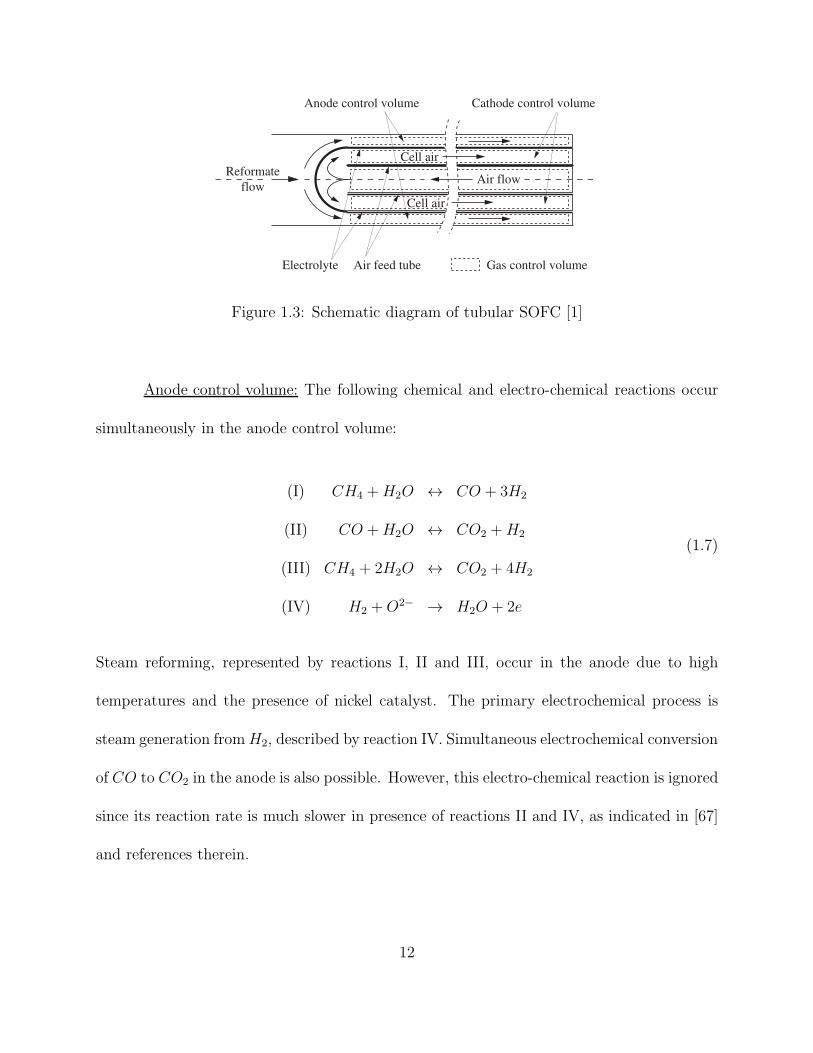
Anode control volume: The following chemical and electro-chemical reactions occur
simultaneously in the anode control volume:
(I) CH4 +H2O ↔ CO + 3H2
(II) CO +H2O ↔ CO2 +H2
(III) CH4 + 2H2O ↔ CO2 + 4H2
(IV) H2 +O2− → H2O + 2e
(1.7)
Steam reforming, represented by reactions I, II and III, occur in the anode due to high
temperatures and the presence of nickel catalyst. The primary electrochemical process is
steam generation fromH2, described by reaction IV. Simultaneous electrochemical conversion
of CO to CO2 in the anode is also possible. However, this electro-chemical reaction is ignored
since its reaction rate is much slower in presence of reactions II and IV, as indicated in [67]
and references therein.
12

From Fig.1.1, the mass balance equations for CH4, CO, CO2, H2 and H2O can be
written as
NaX1,a = −NoX1,a + NinX1,r +R1,a
NaX2,a = −NoX2,a + NinX2,r +R2,a
NaX3,a = −NoX3,a + NinX3,r +R3,a
NaX4,a = −NoX4,a + NinX4,r +R4,a − re
NaX5,a = −NoX5,a + NinX5,r +R5,a + re
(1.8)
where Na = PaVa/RuTa and re is the rate of electrochemical reaction given by
re =iNcell
nF(1.9)
Since current i can be measured, the rate of electrochemical reaction re is considered known.
As with the reformate control volume, the anode inlet and exit flows do not contain O2 and
N2. Therefore, X6,a = X7,a = 0. From Eq.(1.7), we express Rj,a, j = 1, 2, · · · , 5, in terms of
the reaction rates rI , rII and rIII as follows
Ra = Gr+ re [0 0 0 − 1 1]T (1.10)
where Ra = [R1,a R2,a R3,a R4,a R5,a]T , and G and r are given in Eq.(1.3). Since G has a
rank of 2 and re is known, therefore there are only two independent reaction rates among
13

Rj,a, j = 1, 2, · · · , 5. Considering R1,a and R2,a to be independent, we can write
R3,a = −R1,a −R2,a,
R4,a = −4R1,a −R2,a − re,
R5,a = 2R1,a +R2,a + re
(1.11)
and rewrite Eq.(1.8) as
NaX1,a = −NoX1,a + NinX1,r +R1,a
NaX2,a = −NoX2,a + NinX2,r +R2,a
NaX3,a = −NoX3,a + NinX3,r −R1,a −R2,a
NaX4,a = −NoX4,a + NinX4,r − 4R1,a −R2,a − re
NaX5,a = −NoX5,a + NinX5,r + 2R1,a +R2,a + re
(1.12)
From Eq.(1.12) we deduce that
No = Nin +
7∑
j=1
Rj,a ⇒ No = Nin − 2R1,a (1.13)
Cathode control volume: Ionization ofO2 in the cathode control volume occurs through
the reaction
0.5O2 + 2e → O2− (1.14)
14

with the reaction rate as given in Eq.(1.9). Considering the mole fractions of N2 and O2
in air to be 0.79 and 0.21 respectively, the mass balance equations of the cathode control
volume can be written from Eqs.(1.9) and (1.14) as follows:
NcX6,c = 0.79Nair −(
Nair − 0.5re
)
X6,c
NcX7,c = 0.21Nair −(
Nair − 0.5re
)
X7,c − 0.5re
Xj,c = 0, j = 1, 2, · · · , 5
(1.15)
More details about the other features of this model can be found in [1, 3].
1.2.3 Fuel Utilization U
Fuel utilization U is mathematically defined as, [13, 21, 20]:
U , 1−No (4X1,a + X2,a + X4,a)
Nin (4X1,r + X2,r + X4,r)(1.16)
where, X1,a, X2,a, X4,a and X1,r, X2,r, X4,r are the molar concentrations of CH4, CO and H2
in the anode and the reformer respectively and No and Nin are shown in Fig.1.1. Eq.(1.16)
is based on the observation that a CH4 and a CO molecule can yield at most four molecules
and one molecule of H2 respectively, as indicated by reactions I, II and III in Eq.(1.7).
Having done some algebra [3, 2], the steady-state utilization Uss is obtained as [3]
Uss =1− k
(
4nFNf/ifcNcell
)
− k(1.17)
15

Note that Eq.(1.17) is independent of the reaction rates R1,r, R2,r, R1,a R2,a and the flow
rates Nin, No. Equation (1.17) is valid in steady-state and is invariant with respect to
variations in operating temperature, operating pressure, mass of reforming catalyst, air flow
rate and operating Steam-to-Carbon ratio [1]). Thus, Eq.(1.17) represents an invariant
relationship between steady-state fuel utilization Uss, fuel cell current ifc, and fuel flow rate
Nf . Given a target Uss, it can be used to determine Nf if ifc is known and vice-versa [3].
The invariant property can serve as an open-loop control for constant utilization
operation. However, it is a steady-state property and hydrogen starvation must be prevented
even during transient operation. Typically, U must be around an optimal value (≈ 85%)
within narrow limits (±5%) even under significant power fluctuations. The limitation of
using the invariant property alone in an open-loop control is demonstrated in simulations
presented in the following sections where instantaneous changes in power demand are applied
through step-changes in current demand ifc,d.
1.2.4 Addressing Transient Performance Using Invariant Property
To demonstrate the SOFC’s vulnerability to current draw without proper control,
a simulation result is depicted in Fig. 1.4. Here, we have considered a tubular SOFC
model, with 50 cells connected in series, each cell having a length of 251cm,fuel flow of
7 × 10⁻⁴moles/s and a current draw of 10A for t < 150s. Using these values, U will be
approximately 85%. It is shown that fuel cell is not even able to endure a 1A increase in
current load due to hydrogen starvation. This result shows the importance of a proper con-
16

trol as fuel cell performance can be easily disturbed facing small perturbations [2].
To address this issue, we refer to [3] in which this transient issue was discussed in details;
However, to demonstrate the motivation for this work, we review how this problem was
solved in [3] briefly.
0 100 200 3009
10
11
12
0 100 200 30060
70
80
90
100
0 100 200 30020
30
40
50
60
time (s) time (s) time (s)
i fc
(A)
U (
%)
Vfc
(V
)
10.5
11
(a) (b) (c)
Figure 1.4: Open-loop Response to Transient Current Demand [2]
For a desired steady-state utilization Uss, and a given demanded fuel cell current ifc,d,
a fuel flow demand Nf,d can be calculated from Eq.(1.17), given by,
Nf,d =ifc,dNcell
4nFUss
[1− (1− Uss)k] (1.18)
Note that as is shown in Fig.1.1, the Fuel Supply System (FSS) provides fuel flow Nf in
response to the demand Nf,d, and Eq.(1.18) ensures that at steady-state U = Uss. However,
during transience, due to the lag associated with the FSS, Nf,d 6= Nf . This results in
fluctuations in U around Uss. Large changes in ifc,d can result in hydrogen starvation (U →
100%). This is illustrated through simulation results shown in Fig. 1.6(a1-d1). To address
this issue, we propose the current regulation method by reversing Eq.(1.18) to calculate the
17

regulated current based on the actual fuel flow, Nf , given by
ifc =4nFUssNf
Ncell
1
[1− (1− Uss)k](1.19)
This current regulation approach as well as lags associated with fuel flow are illustrated in
Fig.1.5 with the switch position labeled CR.
Fuel
supply
system
(FSS)
Controller
Fuel cell stack
and
Power electronics
FUEL CELL SYSTEMNf,d
sensed Nf
ifc,dEq.(3)
Eq.(4)ifc (current drawn)
NfReformer
Mass Flow Sensor data/command flow
CR
OL
D1
D2
Figure 1.5: Transient Control of U through Current Regulation
In comparison, the open-loop (i.e. unregulated current) approach corresponds to the
switch position OL. The proposed current regulation method has similarities with existing
model-based approaches for PEMFC and SOFC systems using current filter or load governor,
[30, 32, 29]. Note that CR assumes no knowledge of the dynamic characteristics of the FSS.
Improvement in transient response of U in CR over OL is depicted in Fig.1.6. Details of
the simulations and the model can be found in [3, 1]. As shown, CR allows significantly
greater fluctuations in load compared to OL, Figs.1.6(a1) and (a2), before the onset of fuel
starvation, Figs.1.6(c1) and (c2).
18

0 100 200 300
10
14
18
22
140 180 22020
30
40
50
0 100 200 3000.5
1
1.5x 10
−3
84
88
92
96
100
140 160 180
i fc
= i
fc,d
(A
)
U (
%)
Vfc
(V
)
14
11
18
22
Nf
(mole
s/s)
Transient departures
from target Uss
Fuel starvation
Voltage
loss
130 150 17010
20
30
40
50
140 160 18020
30
40
50
130 150 1700.5
1.5
2.5
3.5
x 10−3
150 155 160 16581
83
85
87
89
time (s) time (s) time (s) time (s)
U (
%)
Vfc
(V
)
Nf (m
ole
s/s)
Nf,difc,d
18
30
50
(a1) (b1) (c1) (d1)
(a2) (b2) (c2) (d2)
Open Loop (OL)
Current Regulation (CR)
i fc
(≠ i
fc,d
) (A
)
Figure 1.6: Simulations showing Transient Control of U , (from [3])
However, this approach also creates a disparity between ifc,d and ifc during transients
(see Fig.1.6(a2)). This implies that while current regulation protects the fuel cell from fuel
starvation due to power fluctuations, it results in a disparity between the demanded and
delivered power during transients. This disparity amounts to deficient load-following, that
is addressed by hybridizing the fuel cell with an ultra-capacitor.
1.3 Motivation
In many cases, it is needed to design the control inputs such that the output is
independent of one of the exogenous inputs. Specifically, this is the case for SOFCs in
which the actual fuel flow rate is governed by power demand, which is an exogenous input.
Therefore, we want to design the control input, namely the current draw from the fuel cell,
in a way that U undergoes minimum transient fluctuations in the presence of load transients.
19

One could argue that this could be done by sensing the molar fractions of different species
in different locations inside the cell; In other words, measuring U at any instant and then
designing the controls accordingly. Granted this option is possible, it requires too much
intrinsic sensing within the cell which can be very expensive as well as difficult to implement.
Furthermore, estimating U is another possibility through which a control scheme can be
developed. Yet, that requires a comprehensive model, and state estimator performance
would be largely governed by the accuracy of the plant model, which is very approximate in
this case. Hence, the challenge and also the novelty of this work is to control the transients
of the output while no instantaneous information of the system is provided but the steady
state information.
As is shown in Fig.1.6, the transient response of the system is within an acceptable
range even though not much information was provided except the steady state equation of
the fuel utilization (output). This observation prompted us to think whether this method
could be generalized to other cases where the transient control is needed for plants for which
not much information is provided. Further discussion and details on this problem can be
found in chapter 3.
On the other hand, when it comes to SOFC hybrid networks, the concept of decen-
tralized control is fairly novel in the domain of power grids and control systems. The novelty
of this work lies within the simplicity and practicality of the energy conservation method
which is the essence of the developed controllers here. Moreover, lack of any communication
between controllers enables the control scheme to be scaled up to a much broader network
20

with multiple elements.
1.4 Contributions and Objectives
The objectives and contributions of this work can be summarized as follows:
1. Propose a novel method for perfect transient control for a multivariable system for
which sensing or estimation is not available.
2. Prove the invariance of a general parameter under steady-state condition whose mon-
itoring is vital to the health of reformer.
3. Develop a decentralized control scheme for hybrid power network consisting a single
SOFC and an Ultra-capacitor.
4. Develop separate controllers for FC side an UC side without any direct communication.
5. Verify the developed controllers in simulations.
6. Verify the developed controllers on an experimental test-stand.
1.5 Dissertation Overview
In this Dissertation, after discussing some preliminaries and reviewing the existing
works related to the subject in Chapter 1, in Chapter 2, we introduce STCR and STCB
that are highly important to be monitored to guarantee a safe operation in the reformer.
21
Then, we prove some facts about those parameters and outline their importance in the safe
operation of the SOFC System. Consequently, in Chapter 3,we initially present a review of
output controllability criteria which potentially could be related to the problem which we
have formulated and discussed later on in this chapter. Then, we focus on the transient
control of U as a theoretical problem. We show through both analysis and simulations that
a generalized abstraction of the transient control problem in SOFCs is possible. The main
idea is that in a multi-input single output system, under certain conditions, it is possible
to achieve complete isolation of the output from exogenous input(s) by shaping control
inputs, even if the plant is largely unknown or partially known and the output variable itself
is not measurable. Such a generalized problem can be posed for non-linear time-varying
systems and also for linear time invariant systems. For the latter category of systems, we
derive analytical conditions under which the problem is solvable. We also show how these
conditions are somewhat satisfied by the fuel cell system, and consequently yield acceptable
transient control of U even though the SOFC system is non-linear and time-varying. On the
other hand, a brief review of decentralized control and the motivation of this work will be
presented in Chapter 4. Then, it will be followed by a concise description of the fuel cell
model and its hybridization with ultra-capacitor is presented. Then, the theory and concept
of decentralized approach which we have employed will be explained. Next, separate local
controllers for each fuel side and ultra-capacitor side will be introduced. A conservation of
energy based controller for fuel cell side and two separate controllers for the ultra-capacitor
side will be outlined. The first FC side controller leads into gradual over-charging of the
22

ultra-capacitor which mandates energy dissipation to adjust the UC state of charge. On
the other hand, out of two proposed controllers for UC side, one uses a PWM circuit to
dissipate extra energy, and the other uses voltage modulation to tailor the capacitor’s stored
energy. In the latter approach, the FC observes the manipulated voltage and interprets
that information to gradually decrease uncertainties over time. Following to the theoretical
discussion, the experimental results are presented as well to verify the proposed controllers’
performance.
Finally, the document is concluded with a summary of what has been done throughout the
entire research we have conducted in chapter 5. Thereafter, the references are provided.
23
CHAPTER 2INVARIANT PROPERTIES IN FUEL CELL
1
2.1 Chapter Overview
In order to avoid carbon deposition and catalyst degradation, reformer needs to access
sufficient steam to carry on the reforming reaction. Steam to carbon ratio (STCR) is an
index indicating availability of the steam in the reformer. In this chapter, we first define a
new variable called steam to carbon balance (STCB) based on STCR, and show that for
steam reformer based SOFCs which utilize Methane as the main fuel, the steady-state STCB
is invariant with respect to internal flow rates, reaction rates, temperatures and pressures.
It is shown that STCB is only dependent on the input fuel flow rate and current draw
through simple algebraic relationships. Using invariant relationships, the steady-state fuel
utilization and STCB can be maintained at a target value and its transient fluctuations can
be attenuated.
1The contents of this chapter have been previously published [68]
24

2.2 Analysis of Steady-State Steam to Carbon Balance
2.2.1 Definition and Significance of STCR
Carbon deposition which is a common issue in SOFCs [37, 38], can be jeopardizing
the health of catalysts in both reformer and anode [69]. Many works has been done by
researchers to address this issue. While some have developed control strategies that are
sensitive with respect to carbon deposition [70], Others have focused on different types of
fuels other than H2 [71, 72]. Another case in point is to control the carbon deposition using
STCR. While U is a vital parameter determining the health of fuel cell, Steam-To-Carbon-
Ratio (STCR) plays similar role in the reformer. The effect of STCR on the performance
of SOFC has been experimentally investigated in [73]. On the other hand, STCR seems to
be a rather complicated variable to control. With the aid of simulation, authors in [74] have
shown that several fuel cell variables have significant effect of the STCR. Moreover, it was
observed that there are considerable nonlinearities between the STCR and certain variables
including inlet fuel pressure and system pressure [74].Therefore, to ensure having sufficient
steam to react with Carbon atoms preventing deposition, steam to carbon ratio (STCR) is
defined as follows:
STCR ,Net amount of Steam at the Inlet of SR
Net amount of Carbon Atoms at the Inlet of SR(2.1)
25

Therefore, Referring to Fig.1.1 and Eq.(2.1), for a Methane based steam reformer, STCR is
defined as
STCR =kNoX5,a + NstXst
Nf + kNoX1,a + kNoX2,a
(2.2)
As is indicated by Eq.(2.2)[1], STCR is the ratio of the concentration of steam molecules
to that of carbon atoms at the inlet of the reformer. It is noteworthy that STCR is an
important factor in determining the health of the reformer. Similarly, fuel utilization U can
be used as an index of the health of the fuel cell stack. Therefore, while it is highly impor-
tant to maintain U within limits, it is equally important to monitor STCR to guarantee the
performance of the reformer.
Based on Eq.(1.1), it is evident that the stoichiometric quantity of steam required for re-
forming 1 mole of CH4 and CO is 2 moles and 1 mole, respectively. With this observation,
for a Methane based SR, authors in [1] defined a new variable called steam to carbon balance
(STCB) as follows:
STCB = kNoX5,a + NstXst − (2Nf + 2kNoX1,a + kNoX2,a)
= kNo(X5,a − 2X1,a − X2,a) + NstXst − 2Nf
(2.3)
Essentially, STCB represents the total amount of steam provided to the reformer, subtracted
by the total amount of steam potentially consumed by both fuel and recirculated flow. Similar
to STCR, all the calculations for the STCB are taking place at the inlet of reformer. With
that being said, one can conclude that a positive value of STCB is desirable to prevent
26
carbon deposition [1].
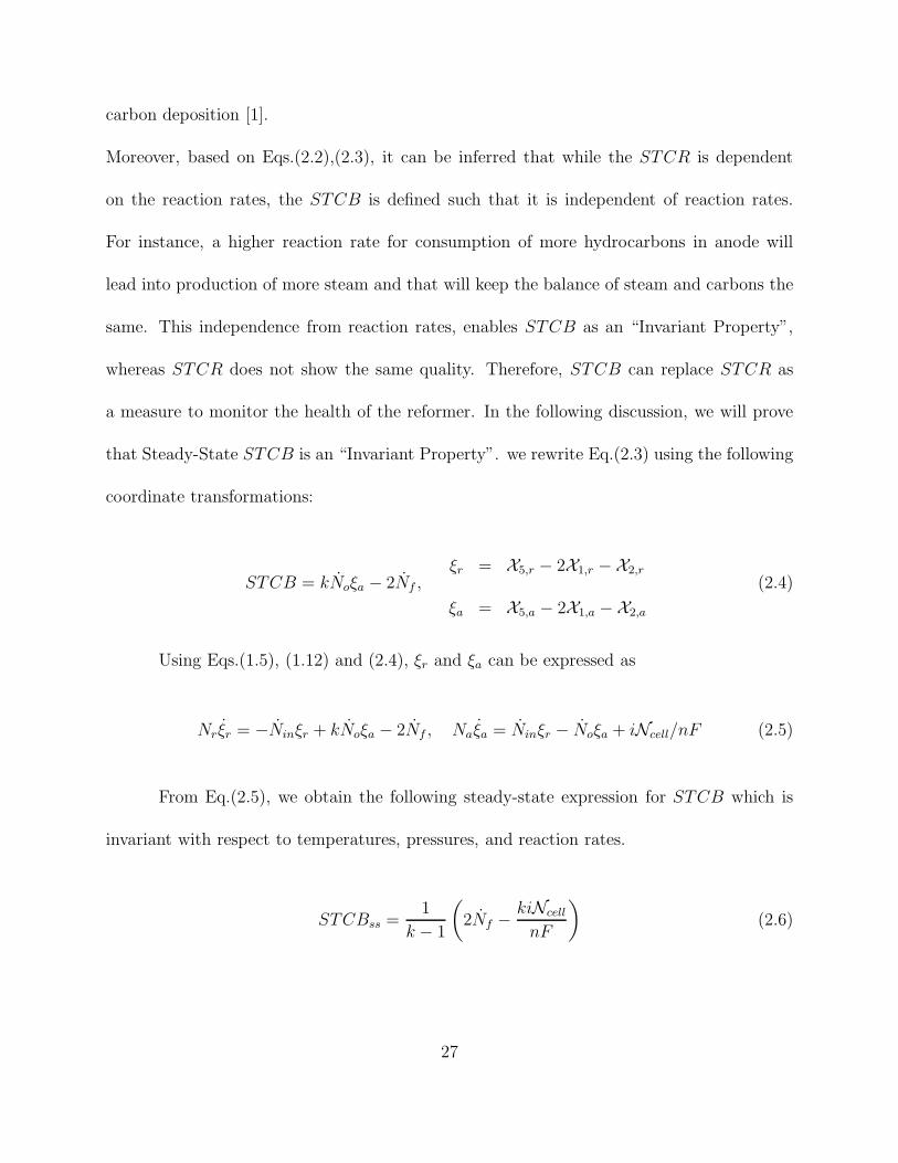
Moreover, based on Eqs.(2.2),(2.3), it can be inferred that while the STCR is dependent
on the reaction rates, the STCB is defined such that it is independent of reaction rates.
For instance, a higher reaction rate for consumption of more hydrocarbons in anode will
lead into production of more steam and that will keep the balance of steam and carbons the
same. This independence from reaction rates, enables STCB as an “Invariant Property”,
whereas STCR does not show the same quality. Therefore, STCB can replace STCR as
a measure to monitor the health of the reformer. In the following discussion, we will prove
that Steady-State STCB is an “Invariant Property”. we rewrite Eq.(2.3) using the following
coordinate transformations:
STCB = kNoξa − 2Nf ,ξr = X5,r − 2X1,r − X2,r
ξa = X5,a − 2X1,a − X2,a
(2.4)
Using Eqs.(1.5), (1.12) and (2.4), ξr and ξa can be expressed as
Nrξr = −Ninξr + kNoξa − 2Nf , Naξa = Ninξr − Noξa + iNcell/nF (2.5)
From Eq.(2.5), we obtain the following steady-state expression for STCB which is
invariant with respect to temperatures, pressures, and reaction rates.
STCBss =1
k − 1
(
2Nf −kiNcell
nF
)
(2.6)
27

2.2.2 General Steady-State Expression of STCB for SR-SOFC System
In this section, we perform some matrix analysis on STCB which was similarly applied
on U in [75, 68]. We first, introduce the conservation of mass for an individual species in a
generic gas control volume, denoted by subscript g, can be derived from first principles as:
d
dt(NgXj,g) = NenXj,en − NexXj,g +Rj,g (2.7)
where, j = 1, 2, 3, ... represents individual species in the gas flow. Rj,g is the net rate
of formation of species j in mol/s due to all chemical reactions in the control volume. The
subscripts en and ex denote the streams entering and exiting the control volume respectively.
It is assumed that the stream leaving the control volume and the control volume itself have
the same composition Xj,g, j = 1, 2, 3, ... . The conservation of mass equation for the gas
mixture is obtained from Eq.(2.7),
d
dt(NgXg) = NenXen − NexXg +Rg (2.8)
where,
Xg = [X1,g X2,g X3,g · · · ]T , Xen = [X1,en X2,en X3,en · · · ]T , Rg = [R1,g R2,g R3,g · · · ]T
(2.9)
In Eq.(2.9), it is noted that the indices 1, 2, 3, ..., represent individual species in the gas flow
and hence the same sequence is used to present species molar fractions in vectors Xg and
28
Xen. On The other hand, to represent STCB in a matrix form, we define a Q matrix such
that
STCB = kNoQTXo + NstQ
TXst + NfQTXf (2.10)
where for the case of Methane-based SR, Q can be found as
QT = [−2 − 1 0 0 1] (2.11)
By definition, Q is a column vector containing the net available steam subtracted by the
potential steam consumed by Carbon atoms. Next, we attempt to obtain the steady-state
STCB by focusing on the mass balance of the reformer and Anode control volumes. The
mass balance of the available steam in the gas control volume can be found by pre-multiplying
Eq.(2.8) with QT. This results in an equation for the conservation of mass of Available Steam
as follows,
NgQTXg +NgQ
TXg = NenQTXen − NexQ
TXg +QTRg (2.12)
Considering steady-state conditions, the left hand side of Eq.(2.12) goes to zero, giving
0 = NenQTXen − NexQ
TXg +QTRg (2.13)
Next Eq.(2.13) will be applied for SR and anode control volumes and then in conjunction
with Eq.(2.10) will yield an expression for the steady-state STCB.
As was mentioned before, considering the SR control volume, there are three inlet flows, the
29

pre-reformed fuel Nf with species concentrations Xf which is considered known, steam Nst
with concentrations Xst where the entries of this vector are zero excepting for the entry cor-
responding to concentration of steam which is 1, and kNo with concentrations Xo. Applying
Eq.(2.13) for SR control volume gives:
0 = NfQTXf + NstQ
TXst + kNoQTXo − NinQ
TXin +QTRSR (2.14)
where RSR represents a column vector containing rate of formation of each species through
steam reforming reactions. We next make the following observation. The chemical reactions
in the SR do not change the total steam available in the gas mixture, they only change
the form from higher hydrocarbons to lower hydrocarbons and hydrogen molecules. Hence,
assuming Q is formulated correctly, QTRSR = 0. This simplifies Eq.(2.14) to,
0 = NfQTXf + kNoQ
TXo + NstQTXst − NinQ
TXin (2.15)
When applying Eq.(2.13) to the anode, Rg = Ra will be a column vector containing the
rates of formation of all species. The reactions include both the electrochemical reaction
Eq.(1.7) and internal steam-reforming reactions. Hence
Rg = Ra = Ra,SR +Ra,e ⇒ QTRg = QTRa = QTRa,SR +QTRa,e = QTRa,e = re (2.16)
30

where Ra,SR and Ra,e contain the rates of internal steam reforming reactions and electro-
chemical reactions respectively. Eq.(2.16) is valid because the only chemical reaction that
affects total steam in the flow is the electrochemical reaction. Equation (2.13) thus reduces
to
0 = NinQTXin − NoQ
TXo + re (2.17)
From Eqs.(1.9), (2.15), (2.17) and Eq.(2.10), the steady-state STCB is expressed as
STCBss =1
1− k[NfQ
TXf + NstQTXst +
kiNcell
nF] (2.18)
Note that in Eq.(2.18), i, Nf , Nst are inputs and Ncell, n, F , k and Xf are known quantities.
Hence, if the vector Q can be obtained, then one can predict STCBss for any set of input
conditions for an SR-SOFC system without knowledge of the rates of reforming reactions,
internal flow rates, temperatures and pressures.
2.3 Control of Fuel Cell Using Invariant Property
2.3.1 Control Scheme Via STCBss
Transient Control of SOFC system based on the constant U has been previously
discussed in section 1.2.4. Similar to that discussion, STCBss expression can replace the Uss
to regulate the current based on the fuel rate Nf and STCBss. In other words:
Nf = gIR(STCBss)ifc (2.19)
31

where for the Methane-based SR-SOFC system, Eq.(2.19) translates into:
Nf =1
2[(k − 1)STCBss + ki
Ncell
nF] (2.20)
Inverting Eq.(2.20) will yield the expression for the shaped FC current draw which guarantees
operation at a pre-specified STCBss value. Simulation results demonstrated in Fig.2.1 shows
how the SOFC system behaves under the STCB-based current regulation approach.
300 400 5001.8
1.9
2
(a)
Time (s)
ST
CR
300 400 500
0
10
20x 10
−5(b)
Time (s)
ST
CB
300 400 500
83
84
85
86
(c)
Time (s)
U(%
)
300 400 500
8
10
12
14
16(d)
Time (s)
i fc (
A)
Figure 2.1: Simulation Results for STCB-Based Current Regulation Approach
Comparing Fig.2.1 and Fig.2.2 (a)-(c) which depicts simulation results using Uss-
based current regulation, it can be deduced that system looks more stable using Uss-based
current regulation. In other words, while STCB and STCR look completely under control
in both approaches, U seems to be not very stable in the STCB-based approach. This
observation can be attributed the the nonlinear nature of the U which mandates a proper
control scheme to make it under control. Thus, the Uss approach which was briefly discussed
in section 1.2.4, and extensively discussed in [3] is a better control scheme compared to the
STCB-based method.
32

2.4 Performance Criteria for the Reformer and Fuel Cell Stack
2.4.1 STCR and STCB at the Stack
Before going into further details, one could raise the same concern of the possibility
of carbon deposition inside the stack (anode). That is to say, how can we guarantee that
there is enough steam to prevent carbon deposition inside the anode as the same species
exist in the anode as well. To respond, we define the STCR at the anode as follows:
STCRa ,Net amount of Steam at the Inlet of Anode
Net amount of Carbon Atoms at the Inlet of Anode(2.21)
Please not that while the major content of CH4 and CO has been consumed in the SR,
in addition to the steam that is fed to the stack by the SR exhaust flow, the electrochem-
ical reaction is constantly producing steam which is favorable from the STCR and STCB
standpoint. Therefore, for a Methane based steam reformer, STCR at the anode is defined
as
STCRa =NinX5,r + reXst
NinX1,r + NinX2,r
(2.22)
Similarly, STCB at the anode can be defined as:
STCBa = NinX5,r + reXst − 2NinX1,r − NinX2,r (2.23)
It can be predicted based on Eqs.(2.22), and (2.23) that there is a considerable margin
of safety in the anode with respect to STCR and STCB. Convincingly, the Simulation
33

results depicted in Fig.2.2 demonstrate that for a Methane-based SR with no external steam
injection, the necessity of monitoring STCB in the SR is much more compared to that of
the stack as for even a small step change in current draw, STCBSR falls below zero which
is detrimental to the health of the SR.
1.85
1.95
2.05
ST
CR
− R
efo
rmer
(a)
0
10
20
x 10−5
ST
CB
− R
efo
rmer
(b)
84
85
86
U (
%)
(c)
300 400 500
4.3
4.4
4.5
4.6
Time(s)
ST
CR
− A
no
de
(d)
300 400 5002
3
4
x 10−3
Time(s)
ST
CB
− A
no
de
(e)
300 400 500
8
10
12
14
16
Time(s)
i fc (
A)
(f)
300 400 500
Time(s)
300 400 500
Time(s)
300 400 500
Time(s)
)
Figure 2.2: Comparison of STCR and STCB for Both Reformer and Stack
2.4.2 Performance Challenges
As is mentioned in section 1.2.4, Uss expression is employed to shape the current based
on the actual fuel flow, given a fixed Uss value. This way, while operating at constant steady
state fuel utilization, the fluctuations of the U is minimized and the health of the fuel cell
stack is guaranteed during even significant transients. However, to make sure the reformer is
also operating in the safe region, it is vital to ensure STCB lies within the acceptable range.
34

First, given the control strategy detailed at section 1.2.4, to ensure constant Uss, the following
needs to be satisfied:
Uss =1− k
(nFNfPTXf/iNcell)− k(2.24)
In other words, since n,F ,k, and Ncell are all constants, to maintain a fixed Uss,
NfPTXf/iD = C1 = const. (2.25)
where D = Ncell/nF is a constant. On the other hand, referring to Eq.(2.18), assuming no
external steam feeding, to keep a fixed STCBss,
NfQTXf + NstQ
TXst + kiD = C2 = const. (2.26)
Therefore, simplifying Eq.(2.26) using Eq.(2.25),
NfQTXf +
k
C1NfP
TXf + NstQTXst = C2 = const. (2.27)
Since all the components in the Eq.(2.27) are constant except Nf , and Nst, it is evident that
Eq.(2.27) cannot hold true. Therefore, with the current control methodology that keeps Uss
at a fixed value, STCBss cannot be fixed. Therefore, the challenge is to find a way that can
guarantee the healthy performance of both reformer and Stack at the same time.
35

2.4.3 Healthy Performance Criteria
Referring to Fig.2.2(b), and(e), it can be seen that the STCBSR and U behave in
the opposite manners. That is, increasing one leads into decreasing the other and vice
versa; thus, controlling both at the same time can serve as conflicting objectives. Another
observation is that the critical condition where STCBSR falls and U rises happens as a
consequence of increasing the current draw from the FC. Both of these observations can be
justified by looking at our control methodology. That is, since the current regulation method
described in Sec. 1.2.4 is based on delaying the current drawn from the fuel cell based on
the actual fuel flow, this will first cause the fuel flow to increase and with some further lag,
the current produced by FC will also increase. Therefore, any change in the current demand
will first affect the fuel flow, and subsequently, that will be reflected in the actual current
produced in the FC. For instance, referring to Fig.2.2(b), (d) and(e), a current step change
from 10 to 15A will first cause increasing fuel flow in the reformer. That will make STCB
to fall, and U to rise because the added fuel has not broken into hydrogen yet; however, the
increase in current draw means more electricity must be generated and consequently, more
steam will be generated that will be recirculated back to the reformer and make the STCB
to back up. Furthermore, more steam and more fuel in the reformer means more hydrogen
is fed into the anode and that will make U to fall back to its steady state value again.
In order to improve the response of the system during the transients, one could argue that
further lagging the current draw from the fuel cell can decrease transient overshoot and
36

undershoot and be eventually favorable. Fig. 2.3 demonstrates the simulation results for the
previous system using a first order filter with a time constant of τ = 2s acting upon current.
300 400 500
1.6
1.8
2
2.2
Time(s)
ST
CR
(a)
300 400 500
0
10
20
x 10−5
Time(s)
ST
CB
(b)
300 400 500
82
86
90
Time(s)
U(%
)
(c)
300 400 500
8
10
12
14
16
Time(s)
i fc
(A)
(d)
Figure 2.3: Simulation Results for U -Based Current Regulation Approach with Lagged Cur-rent
However, the filter on the current turned out to have an adverse effect on the system
as it not only increased the type of the system to the second order, it increased amount of
undershoot and overshoot of both STCB and U due to slow response of the system.
To address the challenge expressed in the preceding section, our objective is to make sure
STCBss ≥ 0 at all time. Granted, this does not guarantee the STCB not crossing 0 at all,
yet, that issue can be easily solved using an external steam injection into the reformer during
the transients. Therefore, for a Methane-based steam reformer with no external steam feed
we have:
STCBss ≥ 0 ⇒ Nf ≤ k(iNcell
2nF) (2.28)
On the other hand, we have
Uss ≥ 0 ⇒ Nf ≥ k(iNcell
4nF) (2.29)
37

Combining Eqs.(2.28), (2.29), and 0 < Uss < 1 will construct a set of linear inequalities
which is solved in a prior publication [1] from another perspective. In [1], the focus of others
was fuel optimization whereas here, the focus is ensuring a healthy performance for both SR
and stack. Referring to [1], it is concluded that to ensure STCBss ≥ 0 and Uss = Const., it
is necessary to have the following condition satisfied:
k ≥1
1 + Uss(2.30)
That is to say, the recirculation ratio k needs to be tuned based on the Uss to have a safe
performance. This condition will guarantee a positive steady state STCB without the aid
of any external steam feeding.
2.5 Chapter Summary
In this chapter, it was shown that in order to avoid carbon deposition in the reformer
of SOFC systems, it is vital to maintain STCR at a certain level. Therefore, using the
concept of conservation of potential steam, STCB was introduced and proved to be invariant
with respect to majority of operating conditions. Moreover, a general analysis was performed
to obtain the steady state expression of STCB which is valid for all types of reformer based
SOFCs. It was shown through simulations that the problem of carbon deposition does
not exist in anode due to electrochemical reaction. Furthermore, a control scheme using
the STCBss expression was outlined and compared to the aforementioned utilization based
38

control strategy. Finally, the conditions guaranteeing simultaneous safe operation of SOFC
stack and reformer were discussed.
39

CHAPTER 3TRANSIENT CONTROL IN MULTIVARIABLE SYSTEMS
WITH APPLICATION IN SOFC
1
3.1 Chapter Overview
Controlling the transient response of variables for which sensing or accurate estima-
tion is not feasible, and a detailed plant model is also largely unavailable, poses significant
challenges. It is a situation that is true in solid oxide fuel cells. In SOFCs, transient control
is essential for fuel utilization, especially if the fuel cell is to be operated in a dynamic load-
following mode at high fuel utilization. The objective is to design the control input(s) such
that it isolates the output (fuel utilization in this case) from measurable disturbances, while
the plant itself maybe largely unknown. The features assumed known are the output’s func-
tional dependence on states which is essentially the output definition, and the steady-state
equation relating the multiple inputs and the output of interest. Simulations have shown
good disturbance rejection in fuel utilization through input shaping. This idea is abstracted
to linear multi-variable systems to provide conditions when this approach is applicable. The
analysis is carried out in time-domain as well as in frequency domain (through singular value
1The contents of this chapter have been previously published [76].
40

analysis). The type of output variables that are amenable to transient control using this ap-
proach is derived through analysis. It is shown that the fuel utilization, although inherently
nonlinear within the nonlinear dynamics of the fuel cell, has some similarities with the linear
abstraction that leads to the observed transient control.
3.2 Output Controllability
3.2.1 What is Output Controllability?
In the control theory, controllability is a common concept which is usually defined
as the ability of a system to reach any desired state starting from any initial state within a
finite period of time [77]. However, in many engineering applications, it is needed to direct
the output toward some desired value. In fact, having control over the output of the system
has a significant importance if not more than the states. Reviewing the literature, it is
shown that no obvious connection can be verified between state controllability and output
controllability [78, 79].
For a LTI (Linear Time Invariant) system with constant coefficients, controllability can be
defined as follows:
Definition 2.1: A dynamic system
˙X(t) = AX(t) +Bu(t), y(t) = CX(t) (3.1)
where, A ∈ Rn×n, B ∈ R
n×m, C ∈ Rp×n; is called controllable if for any initial state X(0)
and any vector X1 ∈ Rn, there exists a finite time t1 and control u(t) ∈ R
n, t ∈ [0, t1] such
41

that X(t1) = X1[80].
In order to verify the controllability of a system, it is conventional to construct the following
matrix
Co =
[
B AB A2B · · · An−1B
]
(3.2)
It can be mathematically proved that the dynamic system 3.1 is controllable if and only if
rank of Co = n [80, 77].
On the other hand, the concept of “Output Controllability” was first introduced by Brockett
in [81] as “Reproducibility” of the system. By definition, reproducibility refers to the capa-
bility of a system to reach some desired output [81]. In this regard, many different forms of
reproducibility has been defined and discussed on such as functional reproducibility which
refers to the ability of a system to generate some particular time functions; asymptotic repro-
ducibility which is related to the likelihood of reaching a specified behavior over time; and
point-wise reproducibility which implies the possibility of approaching some pre-specified
value of the output subspace at some point in time [81].
In general, the output controllability means that the system’s output can be directed
regardless of its state [82]. According to Brockett, the least restrictive form of reproducibility
is called pointwise reproducibility which is defined as follows:
Definition 2.2: The homogenous response from an initial state α is called pointwise repro-
ducible if for any β > 0 and a finite time τ > 0 there exists a δ(β, τ) such that corresponding
42
to each output y for which
‖y − CX(α, 0, t)‖n < δ(β, τ) (3.3)
there exists a control ‖u‖ < β that mandates CX(α, u, t) = y(t) for at least one value of
t ∈ [0, τ ].
In fact, this is not very restrictive condition as many dynamic systems possess this property
and yet, are not “controllable” in practice [81]. Analogous to state controllability, output
controllability for the LTI systems can be also defined as follows:
Definition 2.3: The dynamic system 3.1 is called output controllable or pointwise repro-
ducible if for any initial output y(0) and any vector y1 ∈ Rp, there exists a finite time t1 and
control u1(t) ∈ Rm, t ∈ [0, t1] such that transfers the output from y(0) to y1 = y(t1)[80].
Similarly, a simple test for verifying output controllability can be obtained by constructing
the following matrix
oC =
[
CB CAB CA2B · · · CAn−1B
]
(3.4)
It is mathematically proved that the dynamic system 3.1 is output controllable if and only
if rank of oC = p [80].
It is noteworthy that the state controllability is dependent on linear differential equation of
states; whereas the output controllability is not only dependent on differential equation of
states, it also is related to the algebraic output equation [80].
43

3.2.2 Functional Output Controllability
Generally speaking, the functional output controllability is related to the ability of a
system to direct its output toward any arbitrary curve over any period of time, regardless
of its states. That is, if it is given a desired output yd(t), t ≥ 0, there exists some t1 and a
control ut, t ≥ 0 such that it mandates y(t) = yd(t) for any t ≥ t1 [82].
Mathematically speaking, functional output controllability, i.e. reproducibility can be de-
fined as follows:
Definition 2.4: The homogenous response from an initial state α is called functionally
reproducible if for any β > 0 and a finite time τ > 0 there exists a δ(β, τ) such that corre-
sponding to each output y for which
‖y − CX(α, 0, t)‖n < δ(β, τ) (3.5)
there exists a control ‖u‖ < β that mandates CX(α, u, t) = y(t) for all values of t ∈ [0, τ ]
[81].
In general, functional reproducibility is a local property as in the above definition, the be-
havior of the dynamic system in the vicinity of the desired solution is investigated.
44
3.2.2.1 Functional Output Controllability in LTI systems
The following theorem which is introduced and proved in [81] expresses the condition
for functional reproducibility or functional output controllability.
Theorem 2.1: Consider the LTI system 3.1 for which all the assumptions for A, B, and C
hold true; All homogeneous responses of this system are functionally reproducible if and only
if the pn× (2mn−m) matrix
Mn =
CB CAB CA2B · · · CAn−1B CAnB · · · CA2n−1B
0 CB CAB · · · CAn−2B CAn−1B · · · CA2n−2B
0 0 CB · · · CAn−3B CAn−2B · · · CA2n−3B
......
... · · ·...
... · · ·...
0 0 0 · · · CB CAB · · · CAn−1B
(3.6)
is of rank pn[81].
Similarly, in [82], the following condition is introduced as the necessary and sufficient condi-
tion for functional output controllability.
rank
C
CA CB
CA2 CAB CB
... · · ·. . .
CAn CAn−1B · · · CAB CB
= (n+ 1)p (3.7)
45

In the frequency domain, it is shown by Brockett in [81] that C(Is− A)−1B is of rank p if
and only if Mn is of rank pn. Analogously, if
rank
sI − A B
C 0
= n+ p (3.8)
the system (A,B,C) is functionally output controllable [82].
Proposition: Consider the following singular system
˙EX(t) = AX(t) +Bu(t), y(t) = CX(t) (3.9)
where E ∈ Rn×n. This singular system is functional output controllable if and only if
rank
sE −A B
C 0
= n + p (3.10)
or rank of C(sE −A)−1B = p[82].
3.2.3 Steady-State Output Controllability
By definition, for system 3.1, if a control vector U is provided such that
limt→∞
y(t) = δ (3.11)
46

where δ is a p × 1 output vector, and δi is a given constant, then this problem is called
constant steady-state output controllability of LTI systems [78, 80].
Definition 2.5: An LTI system like 3.1 is claimed to be stead state output controllable if
an input vector U(s) where ui(s) =kiscan be found that generates a constant desired output
vector δ[78, 80].
Clearly, a mandatory pre-condition for constant steady-state output controllability of the
system is stability of the system [80].
Proposition: A stable system like 3.1 is constant steady-state output controllable if and
only if [80]
rank
A B
C 0
= n +min[m, p] (3.12)
3.2.4 Output Controllability in Nonlinear Systems
Brockett in [81] has established a method for checking the reproducibility of nonlinear
systems by testing its linear terms under some specific conditions.
Consider A,B and C matrices similar to system 3.1; and consider A is Hurwitz. Let M(a)
denote the point set X(t), U(t) : |X(t)| < a, |U(t)| < a. Consider the following nonlinear
system˙X(t) = AX(t) +BU(t) +BR(X(t), U(t))
y(t) = CX(t)
(3.13)
where R(X(t), U(t)) and its partial derivatives with respect to the components of X(t)
and U(t) are continuous in N(a) and disappear when X(t) and U(t) disappear. Then, the
47

following theorem can be proved.
Theorem 2.2: Consider the system 3.13 with the given assumptions on all its components.
Therefore, there exists a β > 0 such that any homogeneous response of the form CX(η, 0, t)
with |η| < β is i) pointwise, or ii) functionally reproducible if all the homogeneous responses
of the linearized system˙X(t) = AX(t) +BU(t)
y(t) = CX(t)
(3.14)
are i) pointwise, or ii) functionally reproducible [81].
3.3 A Generalized Transient Control Problem
From the pre-outlined transient control problem of Solid Oxide Fuel Cells in section
1.3, a generalized transient control problem can be formulated for multi-input single output
(MISO) systems. This generalized problem statement is as follows: Consider a nonlinear
and non-autonomous MISO system described as,
X = f(X, t, u, w), y = h(X, t, u, w) (3.15)
where, X is the state vector, y is the output, u is the vector of control inputs and w is the
vector of disturbance/exogenoues inputs. Let us assume that at steady-state,
yss = g (uss, wss) (3.16)
48

where the subscript ss denotes steady-state. Further, let us assume that the following are
true:
1. The functions h(X, t, u, w) and g (uss, wss) are known but knowledge of f(X, t, u, w) is
“incomplete”.
Note: The exact implication of “incomplete” knowledge of the plant will be clarified
in the problem statements in the following sections.
2. X and y are not measurable, but the exogenous inputs w are measurable.
Then, under what additional condition(s), can we design the control inputs u = q(w) such
that limt→∞ y(t) = δ, where δ is a desired/target value of y?
The above problem corresponds closely to the fuel utilization control problem in
SOFCs, where X corresponds to the states and y corresponds to U , whose functional form
is known as well. Also, Nin, No, Nr, Na, are functions of time, making the system non-
autonomous. Nf is the exogeneous input and ifc, which is shaped based on Nf using
Eq.(1.19), is the control input. Eq.(1.17) corresponds to the function g (uss, wss), assumed
known. Also, δ corresponds to the target Uss. We first formulate the problem for a linear
time invariant(LTI) MISO system.
3.4 Problem Formulation for an LTI-MISO System
Consider the following LTI-MISO system
X = AX +B (u + w) , y = CX (3.17)
49

where A ∈ Rn×n, B ∈ R
n×n, C ∈ R1×n. Also let u ∈ R
n×1 and w ∈ Rn×1 represent
the vectors containing the control inputs and disturbance inputs respectively. Following to
Eq.(3.17), the steady-state input/output relation is therefore
Xss = 0 = AXss + B (uss + wss)
⇒ Xss = −A−1B (uss + wss)
⇒ yss = CXss = −CA−1B (uss + wss)
(3.18)
Next, we make the following assumptions that are parallel to those for the generalized non-
linear time-varying case:
1. B and C matrices are known but A is unknown.
2. A is Hurwitz which can be inferred based on an overall physical knowledge of the
system.
3. B is invertible.
4. There are m < n disturbance inputs in w and (n −m) ≥ 1 control inputs in u. This
implies that the sum of L0 “norms” of u and w is n, which essentially means a total
of n inputs.
5. CA−1B is known.
Note: Knowing C, B and Eq.(3.18) does not imply the knowledge of A.
6. X and y are not measurable, but the exogenous inputs w are measurable.
50

Note that the set of assumptions above now clearly defines what we mean by incomplete
knowledge of f(X, t, u, w) in assumption 1 of the generalized case, but this definition is only
applicable for LTI-MISO systems. The question we ask is, can we design u = q(w) such
that limt→∞ y(t) = δ where δ is a desired/target value? To this end, we give the following
theorem:
THEOREM 1: Consider the LTI system given in Eq.(3.17) for which all the above
assumptions are valid. If y is such that CA−1 and C are linearly dependent, then by using
Eq.(3.18) with
δ = −CA−1B (u + w) (3.19)
we can completely eliminate the effect of w on y and ensure limt→∞ y(t) = δ for any transients
in w.
Proof: First, we observe that since C, B and CA−1B are known and B is invertible,
CA−1 can be determined from the given information. Hence we can verify if C and CA−1
are linearly dependent, without knowing A. If they are, then
CA−1 = αC, α < 0 (3.20)
Here α < 0 because Eq.(3.20) implies
C = αCA ⇒ C
(1
αI −A
)
= 0 (3.21)
51

and hence 1/α is an eigenvalue of A and C is the corresponding eigenvector. Since A is
known to be Hurwitz, α is negative real. Now, taking the derivative of Y , we have
y = CAX + CB (u + w) ⇒ y =1
αy + CB (u + w) (3.22)
which implies that by choosing u to satisfy
CB (u + w) = CBu+ CBw = −δ
α⇒ lim
t→∞
y(t) = δ (3.23)
From Eq.(3.20), CA−1 = αC and therefore by choosing u to satisfy
CA−1B (u + w) = −δ (3.24)
we ensure limt→∞ y(t) = δ. This completes the proof. ⋄ ⋄ ⋄
We note that we are essentially using the steady-state equation Eq.(3.18) to shape u
using the measurements of w to ensure complete disturbance rejection in y. Also, given that
w is measurable, we only need one control input to control the transients in y. Any extra
control input can be used to achieve other control objectives. We also make the following
observations:
Remark 1: Given a MISO-LTI system with B, C and CA−1B satisfying all the
conditions of Theorem 1, there exists a continuum of realizations of admissible A matrices.
Remark 2: A loss of observability is an enabler for transient control of y, since linear
52
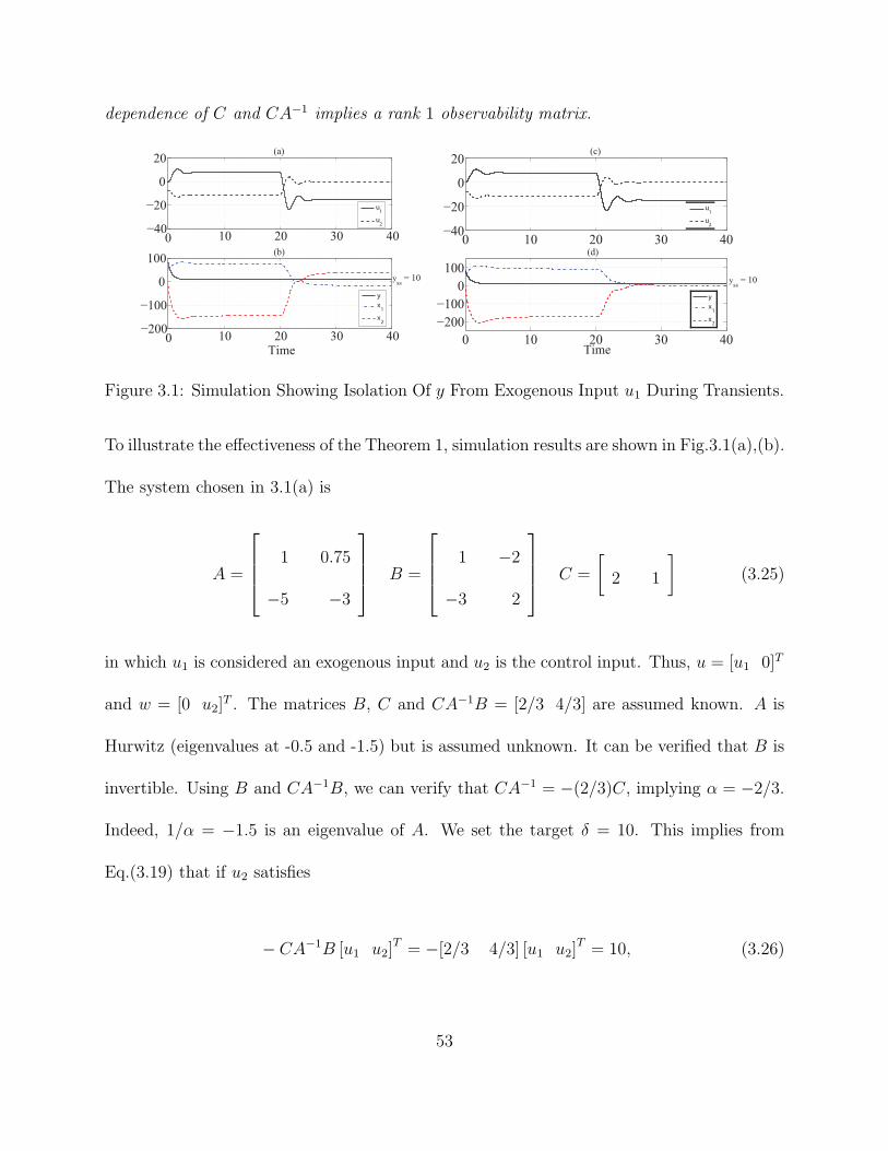
dependence of C and CA−1 implies a rank 1 observability matrix.
0 10 20 30 40−40
−20
0
20
0 10 20 30 40
−200
−100
0
100
(d)
(c)
0 10 20 30 40−40
−20
0
20
0 10 20 30 40−200
−100
0
100
Time
y
x1
x2
u1
u2
yss = 10
u1
u2
y
x1
x2
yss = 10
Time
(b)
(a)
Figure 3.1: Simulation Showing Isolation Of y From Exogenous Input u1 During Transients.
To illustrate the effectiveness of the Theorem 1, simulation results are shown in Fig.3.1(a),(b).
The system chosen in 3.1(a) is
A =
1 0.75
−5 −3
B =
1 −2
−3 2
C =
[
2 1
]
(3.25)
in which u1 is considered an exogenous input and u2 is the control input. Thus, u = [u1 0]T
and w = [0 u2]T . The matrices B, C and CA−1B = [2/3 4/3] are assumed known. A is
Hurwitz (eigenvalues at -0.5 and -1.5) but is assumed unknown. It can be verified that B is
invertible. Using B and CA−1B, we can verify that CA−1 = −(2/3)C, implying α = −2/3.
Indeed, 1/α = −1.5 is an eigenvalue of A. We set the target δ = 10. This implies from
Eq.(3.19) that if u2 satisfies
− CA−1B [u1 u2]T = −[2/3 4/3] [u1 u2]
T = 10, (3.26)
53

for any measured exogenous input u1, then limt→∞ y(t) = 10. This is confirmed in Fig.3.1(b).
In this simulation, initial values X(0) = [50 − 20]T were chosen arbitrarily. At t = 20s
the disturbance input u1 was changed from 8 to −15 with an underdamped second order
dynamics. Note that u2 is shaped using Eq.(3.26).
Moreover, to demonstrate what was mentioned in Remark 1, another simulation was run
using a different A matrix with the same B and C and the same inputs (u1 and u2). In this
case, system was chosen to be
A =
2.5 1.5
−8 −4.5
B =
1 −2
−3 2
C =
[
2 1
]
(3.27)
for which the same exact inputs are implemented. In Fig.3.2 we compare the transient
performance of the system described in Eq.(3.25) with two different choices of C that are
not linearly dependent on CA−1. It can be seen from the Fig.3.2 that with only linearly
dependent C, perfect transient response is achievable while for other options, some deviations
from the steady state value can be observed.
0 10 20 30 40−50
0
50
yss
= 10
Time
yC = [1 1]
C = [2 1]
C = [4 1]
yss
= 10
Figure 3.2: Comparison Of Transient Response For Three Different C Matrices.
54

3.4.1 Complex Conjugate case
So far, we showed the feasibility of transient control for the case where C and CA−1
are linearly dependent. This implies that the depenedence is through a negative real eigen-
value; in other words, A must be Hurwitz. However, one could pose the same question for a
case where A has complex conjugate yet stable eigenvalues. Now, the question rising from
what we have discussed so far is: Considering an LTI-MISO system for which complex con-
jugate eigenvalues are present; Assuming all the aforementioned assumptions hold through,
can we design u = q(w) such that limt→∞ y(t) = δ where δ is a desired/target value. To
answer, we represent the following theorem.
THEOREM 2: Consider the LTI system as described in Eq.(3.17) for which all the as-
sumptions mentioned in Theorem 1 are valid with the exception that y ∈ R2×1, C ∈ R
2×n,
and y is such that
CA−1 = NC (3.28)
where N ∈ R2×2 is of the form of a real jordan block [83] as follows:
N =
α β
−β α
(3.29)
with α < 0, β > 0. Then it is possible to completely eliminate the effect of w on any desired
output, say y1, and ensure limt→∞ y1(t) = δ for any transients in w if the L0 norm of u is
greater than or equal to 1.
Proof : This is a scenario where C is related to CA−1 by a jordan block, N , which implies
55
the existence of complex conjugate eigenvalues in A.
Now, back to Eq.(3.17) and (3.18), for a case with two inputs and two outputs we have
y = CAX + CB(u+ w) ⇒
y1
y2
= CAX + CB(u+ w) (3.30)
Analogous to Eq.(3.21),
C = NCA ⇒ CA = N−1C (3.31)
Subsequently, plugging Eq.(3.31) into Eq.(3.30),
y1
y2
= N−1
y1
y2
+ CB(u+ w) (3.32)
On the other hand, similar to Eq.(3.18), we have
y1ss
y2ss
= −NCB(u + w) (3.33)
Hence, by choosing u to satisfy
δ = M1(u+ w) (3.34)
where
M1
· · ·
M2
= −NCB (3.35)
56

and noting that M1 ∈ R1×n, we ensure that limt→∞ y1(t) = δ. This completes the proof.
⋄ ⋄ ⋄
3.5 Problem Formulation in Frequency Domain
Since we are interested in multi-variable systems, it prompts us to formulate the prob-
lem from singular value/singular vector perspective. Specifically, it is clear that if the input
vector is directed along any of the singular vectors corresponding to σ = 0, then y would be
completely isolated from the exogenous inputs. Thus, the transient control problem can be
posed as follows: Are there conditions under which it is possible to determine a singular vec-
tor corresponding to a zero singular value of the above-mentioned LTI-MISO system without
the knowledge of the A matrix?
Note: A MISO transfer function C(sI −A)−1B will have one or more zero singular values,
i.e. σ = 0.
THEOREM 3: Consider the LTI system described by Eq.(3.17) and (3.18)for which
all the assumptions outlined in the Theorem 1 are satisfied. If y is such that CA−1 and C
are linearly dependent, then the direction perpendicular to CB is the direction of a singular
vector corresponding to σ = 0. Hence, if the input (u+ w) is directed in this direction, then
y will be completely isolated from the effect of disturbance w and ensure limt→∞ y(t) = 0 for
any transient in w.
Proof: Taking Laplcae transform of Eq.(3.17)
57

C(sI −A)X(s) = CB[u(s) + w(s)] (3.36)
Therefore, from Eq.(3.21) we have,
(s− 1α)CX(s) = CB[u(s) + w(s)] ⇒
y(s) = CB 1(s− 1
α)[u(s) + w(s)]
(3.37)
From Eq.(3.37), it can be inferred that if u is designed such that (u(s)+w(s)) is perpendicular
to CB, then complete disturbance rejection can be achieved. This completes the proof. ⋄⋄⋄
Corollary: For the above mentioned system under the same assumptions, any desired steady
state value for the output δ can be obtained, i.e. limt→∞ y(t) = δ.
Proof : With,
CB[u(t) + w(t)] = −δ/α (3.38)
Then referring to Eq.(3.37) We have
y(s) =1
(s− 1/α)(−
δ
α)(1
s) ⇒ lim
t→∞
y(t) = lims→0
−δ/α
s− 1/α= δ (3.39)
Remark Theorem 2 is indeed, the extension of the application of “Zero” in a multivariable
system. According to the definition [84], if G(s) has a zero at s = z, then G(s) loses rank at
s = z and there will exist a non-zero vector uz such that
G(z)uz = 0 (3.40)
58

Where uz is called zero direction corresponding to a zero singular value of G(z). Similar
concept is applied in the Theorem 2; However, the approach in Theorem 2 is more broad
as it works over all frequencies. In other words, the vector of inputs u corresponding to the
zero singular value is shaped such that the output y tends to zero not in a certain frequency
but over all range of frequencies.
3.6 Generalized Transient Control Problem for LTI Systems
Previously, to achieve a perfect transient response in output, we imposed the condition
of linear dependency between C and CA which led into emergence of the output y in the
expression of y. Thereafter, we could design our control input based on the exogenous input
such that the output did not react to any transient in exogenous input. To weaken this
condition, we propose the following theorem:
THEOREM 4: Consider a [2 × 2] LTI system given in Eq.(3.17) for which all the
aforementioned assumptions are valid. Then by knowing A which is Hurwitz, and B and C
matrices, and choosing
[a1C + CA]Bu+ CBu = 0 (3.41)
where a1 is the coefficient of the characteristic equation s2+ a1s+ a2 = 0, we can completely
eliminate the effect of exogenous inputs w on y and ensure limt→∞ y(t) = 0 for any transients
in w.
Proof: We consider the following LTI system:
59

X = AX +Bu, y = CX
y = CX = CAX + CBu
y = CAX + CBu = CA2X + CABu+ CBu
(3.42)
On the other hand, according to Cayley-Hamilton theorem [83], any square matrix A ∈ Rn×n
satisfies its own characteristic equation, i.e.
A ∈ Rn×n −→ Sn + a1s
n−1 + a2sn−2 + · · ·+ an = 0
⇒ An + a1An−1 + a2A
n−2 + · · ·+ anI = 0
⇒ An = −[a1An−1 + a2A
n−2 + · · ·+ anI]
(3.43)
Eq.(3.43) means that the nth power of any square matrix A can be expressed as a linear
combination of the lower powers of A including A0 = I. therefore, from Eqs.(3.42),(3.43) we
have:y = −(a1CA+ a2C)X + CABu+ CBu
⇒ y + a2y = −a1(y − CBu) + CABu+ CBu
⇒ y + a1y + a2y = a1CBu+ CABu+ CBu
(3.44)
Therefore, by knowing A which is Hurwitz, and B and C matrices, Eq.(3.44) leads into a
first order differential equation which can be solved to obtain the desired control input. In
other words, by choosing u and u such that:
[a1C + CA]Bu+ CBu = 0 (3.45)
60

we can guarantee complete isolation of y from the exogenous input. This completes the
proof. ⋄ ⋄ ⋄
To generalize this idea to [n×n] system with characteristic equation of Sn+a1sn−1+
a2sn−2 + · · ·+ an = 0 we define:
On =
C
CA
...
CAn−1
βn =
[
an−1 an−2 · · · a0
]
(3.46)
where O1 = [C] and O2 =
C
CA
, and a0 = 1. Therefore, considering u(0) = u, the
characteristic equation of A ∈ Rn×n leads into
y(n) + a1y(n−1) + a2y
(n−2) + · · ·+ an−1y =
n∑
i=1
βiOiBu(n−i), n ≥ 2 (3.47)
Since A is Hurwitz, by choosing RHS = 0 , it is guaranteed that limt→∞ y(t) = 0 for any
transients in w. To illustrate, we consider the following system:
A =
1 2
−4 −3
B =
1 −2
−3 2
C =
[
2 −1
]
(3.48)
61

A is Hurwitz with eigenvalues Λ1,2 = −1± 2i and characteristic equation is x2 +2x+5 = 0.
Therefore, by simplifying Eq.(3.45) using values at Eq.(3.48), we have:
− 5u1 − 10u2 + 5u1 − 6u2 = 0 (3.49)
in which u1 is considered an exogenous input and u2 is the control input. Simulation results
are depicted in Fig.3.3. it can be seen from Fig.3.3 that the output y, after reaching to
steady state condition, becomes completely isolated from exogenous input u1.
0 5 10 15 20 25 30 35 40
−10
−5
0
5
10
Control Inputs
0 5 10 15 20 25 30 35 40
−10
0
10
20
Time
States and Output
Y
X1
X2
u1u2
Figure 3.3: Isolation Of y From Exogenous Input u1 using Eq.(3.44)
62
3.7 Transient Control in Linearized Fuel Cell Model
Here, we will represent the state space equations for the fuel cell system which will
consist two inputs and one output. we define the states in terms of different mole fractions
as follows:
Z1 = (4X1,a + X2,a + X4,a) , Z2 = (4X1,r + X2,r + X4,r) (3.50)
Therefore, the output equation which results in utilization, in terms of states will be:
U = y = 1−No(t)Z1
Nin(t)Z2
⇒ y = C(Z, t) (3.51)
Using the pre-defined states, the state space equation of the fuel cell system will be as follows:
Z1 = − Nin(t)Z1
Nr(t)+ k No(t)Z2
Nr(t)+ u1
Nr(t)
Z2 =Nin(t)Z1
Na(t)− No(t)Z2
Na(t)− u2
Na(t)
Z1
Z2
=
− Nin(t)Nr(t)
k No(t)Nr(t)
Nin(t)Na(t)
− No(t)Na(t)
︸ ︷︷ ︸
A(t)
Z1
Z2
+
1Nr(t)
0
0 − 1Na(t)
︸ ︷︷ ︸
B(t)
u1
u2
(3.52)
It can be seen from the above equations that fuel cell system is non-autonomous, time
varying with nonlinear output. It is highly demanding to work with such a system. Hence,
to simplify, we linearize the state-space equations around the steady state point as follows:
Note: The magnitude of Na and Nr are in the same order;Thence, for simplicity we neglect
their appearance in the equations.
63

δZ = AδZ + δu
δy = ∂C∂Z
|ssAδZ + ∂C∂Z
|ssδu
(3.53)
Where ∂C∂Z
|ss can be obtained from Eq.(3.51),
∂C
∂Z|ss =
No
NinZ21
[
Z2 −Z1
]
(3.54)
Plugging Eq.(3.54) into Eq.(3.53),
∂C
∂Z|ssA =
No
NinZ21
[
−Nin(Z1 + Z2) No(Z1 + kZ2)
]
(3.55)
Now we would like to verify whether Theorem 1 can be applied to the linearized fuel cell
model or not. Therefore, based on the Theorem 1, linear dependency condition similar to
what was expressed earlier that needs to be satisfied to obtain perfect U response under
transient conditions will be:
α∂C
∂Z|ss =
∂C
∂Z|ssA ⇒ −α
Z2
Z1=
−Nin(Z1 + Z2)
No(Z1 + kZ2)(3.56)
In order to be able to use theorem 1 to justify fuel cell’s transient behavior, we decompose
∂c∂Z
|ssA such that there is a linear dependent part and and a perturbation part. To do that,
we first build the linear dependent part from Eq.(3.56),
64

−Z2
Z1
= − ˙Nin(Z1+Z2)E
⇒
E = NinZ1
Z2
(Z1 + Z2) =No
1−yss(Z1 + Z2)
(3.57)
Now we add and subtract the term E No
NinZ2
1
δZ2 to the Eq.(3.53),
δy =∂C
∂Z|ssAδZ +
∂C
∂Z|ssδu+ E
No
NinZ21
δZ2 − ENo
NinZ21
δZ2 (3.58)
Substituting the second component of ∂C∂Z
|ssAδZ by E No
NinZ2
1
δZ2 and subtracting the replaced
component, we can use Eq.(3.56) and write:
δy =∂C
∂Z|ssδZ − E
No
NinZ21
δZ2 +No
NinZ21
(kZ2 + Z1)δZ2 +∂C
∂Z|ssδu (3.59)
Similar to the Theorem 1, we factor the output out of the Eq.(3.59),
δy = −γδy +No
NinZ21
[
Z2+Z1
1−yss−(kZ2 + Z1)
]
︸ ︷︷ ︸
P
δZ2 +∂c
∂Z|ssδu (3.60)
Eventually, considering the inputs,
δy = −γδy︸ ︷︷ ︸
Homogeneous
+PδZ2 +No
NinZ21
(Z2δu1 − Z1δu2)
︸ ︷︷ ︸
Particular
(3.61)
As γ is a positive number, similar to Theorem 1, the homogeneous part in Eq.(3.59) will
attenuate as time tends toward infinity. Therefore, the question is whether the particular
answer of this differential equation using control input can go toward zero or not?
65

Due to the existence of the perturbation term (P ), the condition of Theorem 1 can not
be met. However, the reason that an autonomous time-varying system such as fuel cell
can have a very acceptable transient response using linear equations is that the magnitude
and significance of the perturbation term in comparison with the control input term is
negligible. Therefore, with designing fuel flow rate based on the current draw, a reasonably
good transient response in U can be achieved.
3.8 Chapter Summary
In this Chapter, a method for controlling transient response of the output of a system
for which sensing or accurate estimation was assumed not to be available, and comprehensive
information regarding plant was not reachable was proposed. First, the area from where this
problem was raised was described. Then it was shown through both analysis and simulation
that under certain conditions, perfect disturbance attenuation is possible. The method was
then verified in frequency domain as well. Thereafter, the conditions under which transient
control was possible were relaxed and a more general Theorem was expressed and proved. At
the end, the approach was applied to fuel cell and similarity and differences were discussed.
It was shown that even though fuel cell system is nonlinear, and time-varying, a linear system
approach can still be applied yielding a reasonable transient response for the output.
66

CHAPTER 4DECENTRALIZED CONTROL FOR A FUEL CELL HYBRID
POWER NETWORK
1
4.1 Chapter Overview
This chapter addresses development of decentralized control scheme for a simple hy-
brid power system consisting of a single fuel cell and an ultra-capacitor. This work devel-
ops separate controllers for the fuel cell and the ultra-capacitor, rather than a centralized
controller. With a goal of developing a control paradigm that is scalable to many energy
resources connected to a network, the controllers are designed primarily to use locally sensed
information. Explicit communication between controllers, such as exchange of locally sensed
information, is absent. An energy conservation based approach, combined with a current
regulation method developed by the authors in their earlier work [3], is used for transient
control of the fuel cell. The control of state-of-charge of the ultra-capacitor is also principally
governed by energy conservation, but implemented using two different approaches. One is
based on dissipation, and the other is based on voltage modulation. The former is a conser-
1The contents of this chapter have been previously published [85, 40].
67

vative approach, while the latter is potentially more energy efficient. Simulation as well as
experimental results are presented to demonstrate these concepts.
4.2 Hybrid Network and Control Objectives
Fig. 4.1 is a schematic of the hybrid system with a decentralized control scheme.
Other approaches for building a fuel cell ultra-capacitor/battery are presented in [10, 12, 35,
86, 87, 3]. In our approach, we assume that fuel cell and the ultra-capacitor are connected
in parallel.
DC/DC
Conv.
(η1)
Fuel Cell
System
K1
Load
Vfc , ifc
C1
VL , iL
Nf,d
. Nf
.
DC/DC
Conv.
(η2, η2)
Storage Device
Ultra-capacitor
C2
K2
Vuc , iuc VL , io
ifc
Figure 4.1: Schematic of Hybrid Fuel Cell System with Decentralized Control
Using a uni-directional DC/DC converter C1, the fuel cell supplies power to the load.
The ultra-capacitor is connected to the load through a bi-directional DC/DC converter C2
allowing charge and discharge. Referring to Fig.4.1, Some features of the hybrid system are:
1. Due to their fast responses, C1 and C2 are assumed to be static energy conversion
devices, with C1 having an efficiency of η1 and C2 having discharge and charge efficien-
cies of η2 and η2 respectively [88, 8]. These efficiencies are bounded, but unknown and
time-varying. We also assume that η2,min ≤ η2, η2 ≤ η2,max. Furthermore, we consider
68

C1 to be operating in current control mode, while C2 maintains voltage VL in a voltage
control mode.
2. Based on the schematic in Fig.4.1, since the fuel cell and the ultra-capacitor are con-
nected in parallel, the following is true at any instant:
VLiL = η1Vfcifc+
[η2 + η2
2+
η2 − η22
sgn(iuc)
]
Vuciuc ⇒
VLiL = η1Vfcifc + η2Vuciuc, iuc > 0
VLiL = η1Vfcifc + η2Vuciuc, iuc < 0
(4.1)
where iuc > 0 and iuc < 0 imply charge and discharge respectively of the capacitor. The
above equation implies that the net power demand VLiL is supplied at every instant.
3. To realize a decentralized control, we impose the following restrictions on K1 and K2.
Controller K1 uses measurements of Vfc, VL, iL, and Nf , commands C1 to draw ifc,
and commands the FSS to deliver a desired fuel flow rate of Nf,d. However, K1 does
not use measurements of iuc, Vuc or η2. This is also indicated in Fig.4.1.
4. As shown in Fig.4.1, controller K2 measures Vuc and iuc only, and does not use mea-
surements of VL, iL, Vfc, ifc or η1. K2 commands C2 to maintain a desired VL.
4.2.1 Control Objectives
Referring to Fig.4.1, and under the operational conditions in section 4.2, the control
objectives are:
69

1. The target fuel utilization at steady state will be Uss = 0.8, and the deviations from
Uss during transients should be minimized [3, 1].
2. Control scheme is designed to maintain the SOC of the ultra-capacitor at the target
value of St.
3. Control the load voltage VL around a nominal value.
4.3 Decentralized Control Using Conservation of Energy Principle
4.3.1 Approach
This work applies conservation of energy to develop decentralized control of the hybrid
system in Fig.4.1. Conceptually, the approach is illustrated in Fig. 4.2.
Time (s)
190 200 210 230 250
300
400
500
600
Po
wer
(w
)
Power Demand (VLiL)
Power Supplied (η1Vfcifc)A2
A1
Figure 4.2: Conservation of Energy Approach
The figure shows a step increase in power demand VLiL and the corresponding load-
following response of the source (fuel cell, η1Vfcifc). The area A1 represents the energy
supplied by the storage device (ultra-capacitor in this case) to make up for the fuel cell’s
70

deficiency in load following mode. Therefore, if the area A2, which represents the extra
energy supplied by the FC, match A1, then not only the load is met, but also the capacitor
will be charged to its original SOC in ideal scenario. Extending this idea, in the transient
response of the SOFC, we denote A1,j = 1, 2, . . . as the areas where the ultra-capacitor is
discharged and A2,q = 1, 2, . . . as the areas where the ultra-capacitor is charged. Then under
ideal charge/discharge, i.e. η2 = η2 = 1, the condition
limt→∞
EA = limt→∞
(∑
j
A1,j −∑
q
A2,q
)
→ 0 (4.2)
ensures the storage element maintains its original energy level at steady-state. Ideally, the
above condition can be fulfilled by K1 without any information about the capacitor by just
ensuring
limt→∞
∫ t
0
P dt = 0, P , (VLiL − η1Vfcifc) (4.3)
In the presence of losses in C2 with discharge and charge efficiencies η2 and η2 respectively,
Eq.(4.2) is modified to
limt→∞
EA = limt→∞
(∑
i
A1,i
η2−∑
k
A2,k
η2
)
→ 0. (4.4)
71

If we assume η2 and η2 to be known then, using P as defined in Eq.(4.3), Eq.(4.4) is
satisfied by K1 by ensuring
limt→∞
Ie = 0, Ie ,
∫ t
0
[η−12 + η−1
2
2+
η−12 − η−1
2
2sgn(P )
]
Pdt (4.5)
where sgn(.) denotes signum function. However, η2 and η2 will be unknown toK1. Therefore,
we need to build a robust control around this principle to handle such uncertainty in a
decentralized manner. The next sections will demonstrate the validity of the main principle.
4.3.2 Implementation and Simulations
To demonstrate that energy conservation can be used in principle to design decen-
tralized control, we consider a simplified scenario. We assume that in addition to the local
information mentioned in Assumption 2, controller K1 has exact knowledge of η2 and η2.
Next, in designing K1, we recall that the commanded ifc must be based on the actual fuel
flow Nf for transient control of U , as detailed in [3]. Also, Nf is driven by the demanded
fuel Nf,d, which in turn is determined from ifc,d. Thus, the command ifc to C1 is determined
as follows:
Nf,d =ifc,dNcell
4nFUssβ ⇒ ifc =
4nFUssNf
Ncellβ, (4.6)
where β = [1− (1− Uss) k]. From Eq.(4.6) we note that designing K1 reduces to the design
of the reference ifc,d. The design of ifc,d is based on the following observation: In load-
following mode, the fuel cell provides the entire power demand at steady-state and uses
72

transient perturbations in power to regulate the ultra-capacitor SOC. With this goal, and
incorporating the approach outlined in section 4.3.1, we formulate ifc,d as:
ifc,d =VLiLη1Vfc
+ giIe, ki > 0 (4.7)
where Ie is defined in Eq.(4.5) and gi is the integral gain. This design is implemented and
simulation results are summarized in Fig.4.3. The parameter values chosen are
C = 25F, η1 = 0.8, η2 = η2 = 0.8, gi = 0.01 (4.8)
The power demand VLiL is subjected to step changes. We note that K2 simply maintains the
constant voltage VL across the load. Fig.4.3(a) confirms the control of SOC and Fig.4.3(b)
plots VLiL and η1Vfcifc.
0.72
0.76
0.8
0.84
SO
C
300
500
700
900
Po
wer
(w
)
200 400 600 800
Time (s)200 400 600 800
Time (s)
(a ) (b)
VLiL
η1Vfcifc
Figure 4.3: Energy Conservation based Control with Known η2 and η2
73
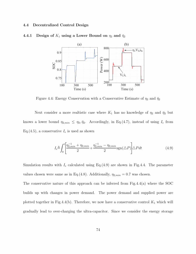
4.4 Decentralized Control Design
4.4.1 Design of K1 using a Lower Bound on η2 and η2
100 300 500
0.75
0.8
0.85
0.9
100 300 500200
400
600
800
SO
C
Pow
er (
W)
Time (s) Time (s)
(a) (b)
VLiL
η1Vfcifc
Figure 4.4: Energy Conservation with a Conservative Estimate of η2 and η2
Next consider a more realtistic case where K1 has no knowledge of η2 and η2 but
knows a lower bound η2,min ≤ η2, η2. Accordingly, in Eq.(4.7), instead of using Ie from
Eq.(4.5), a conservative Ie is used as shown
Ie,
∫ t
0
[
η−12,min + η2,min
2+η−12,min − η2,min
2sgn(P )
]
Pdt (4.9)
Simulation results with Ie calculated using Eq.(4.9) are shown in Fig.4.4. The parameter
values chosen were same as in Eq.(4.8). Additionally, η2,min = 0.7 was chosen.
The conservative nature of this approach can be inferred from Fig.4.4(a) where the SOC
builds up with changes in power demand. The power demand and supplied power are
plotted together in Fig.4.4(b). Therefore, we now have a conservative control K1 which will
gradually lead to over-charging the ultra-capacitor. Since we consider the energy storage
74

device to be of finite capacity, we must regulate the SOC. To address this in a decentralized
manner two approaches are discussed in subsequent sections.
4.4.2 Dissipation Based Approach for Designing K2
iRC R
iuc
Figure 4.5: Dissipation Circuit Schematic
One way to regulate the ultra-capacitor’s SOC is to dissipate the extra energy through
a variable resistance connected to the ultra-capacitor. Granted that this would lead to addi-
tional energy loss, but it is a simple yet effective way to control the SOC. The configuration
for dissipation is shown in Fig.4.5 which is a resistance in parallel with capacitor allowing
K2 to handle the charge-discharge in a decoupled manner. The energy dissipation can be
controlled by K2 by actuating the switch shown in both configurations in Fig.4.5, e.g. using
pulse-width-modulation (PWM). Since the SOC is a local information for K2, charge man-
agement is done locally without any information about the fuel cell. The following equation
represents case (a) in Fig. 4.5:
CVuc = −(iuc + iR), Vuc = −1
C(iuc + VucσR) (4.10)
75
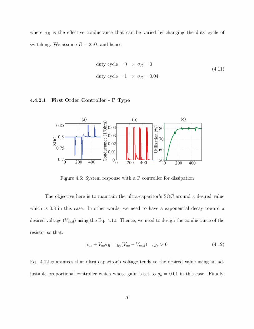
where σR is the effective conductance that can be varied by changing the duty cycle of
switching. We assume R = 25Ω, and hence
duty cycle = 0 ⇒ σR = 0
duty cycle = 1 ⇒ σR = 0.04
(4.11)
4.4.2.1 First Order Controller - P Type
0 200 4000.7
0.75
0.8
0.85
SO
C
(a)
0 200 4000
0.01
0.02
0.03
0.04
Conduct
ance
(1/O
hm
) (b)
0 200 40050
60
70
80
(c)
Uti
liza
tion (
%)
Figure 4.6: System response with a P controller for dissipation
The objective here is to maintain the ultra-capacitor’s SOC around a desired value
which is 0.8 in this case. In other words, we need to have a exponential decay toward a
desired voltage (Vuc,d) using the Eq. 4.10. Thence, we need to design the conductance of the
resistor so that:
iuc + VucσR = gp(Vuc − Vuc,d) , gp > 0 (4.12)
Eq. 4.12 guarantees that ultra capacitor’s voltage tends to the desired value using an ad-
justable proportional controller which whose gain is set to gp = 0.01 in this case. Finally,
76

solving for σR in Eq. 4.12,
σR = gp(1−Vuc,d
Vuc)−
iucVuc
(4.13)
Using the Eq. 4.13, Fig. 4.6 shows that state of charge returns to the desired value within a
reasonable time after the load is implemented no matter step changes are positive or negative.
Not to mention, saturation limits of 0 and 0.04 have been imposed to conductance to make
sure first the resistance does not go to negative values as it does not have any physical
meaning. Furthermore, to ensure resistance does not go to infinity, saturation limits needs
to be enforced.
4.4.2.2 PI Controller
The objective here is to treat σR as a control input and to design a control law that
will stabilize the equilibrium Vuc = Vuc,d and Vuc,d is such that Vuc,d/Vuc,max = 0.8. For
our ultra-capacitor, Vuc,max ≈ 16V and hence Vuc,d = 13V. Since for constant load under
steady-state iuc = 0, a proportional controller of the form σR = [gp,uc(Vuc − Vuc,d)− iuc] /Vuc
will suffice. However, a PI controller will better perform under load variations. Hence, the
following PI control law is proposed:
σR =gp,ucVuc
(Vuc − Vuc,d) +gi,ucVuc
∫ t
0
(Vuc − Vuc,d) dt (4.14)
77

Results for step changes is depicted in Fig.4.7. In contrast to Fig.4.4(a) where the SOC
control was not implemented in K2, the SOC converges to 0.8 with the PI control of Eq.(4.14)
implemented inK2. The manner in which the resistance R is used in the PI controll is evident
from Fig.4.7(b).
(a)
200 300 400 5000.7
0.74
0.78
0.82
0.86
Time (s)
SO
C
(a
200 300 400 500
0
0.01
0.02
0.03
0.04
σR
(O
hm
-1)
(b)
Time (s)
Time (s)
500400300200100200
400
600
800
Po
wer
(W
)
(c)
Figure 4.7: System response with a PI controller for dissipation
The integrator is also held once upper saturation in σR is reached from below or lower
saturation is reached from above. Also, it can be observed that as SOC drops below 0.8, the
resistance switches off and when it exceeds 0.8, the resistance becomes effective.
Comparing Fig. 4.6 (a) and Fig. 4.7(a), it can be seen that SOC returns to desired value to
some extent faster using the PI controller. Although the amount of over charge is relatively
78

more in the second order case, the dissipation phenomenon takes place faster using the PI
controller. The pattern with which the resistance is used in the P and PI controller is
demonstrated in Fig. 4.6 (b) & Fig. 4.7(b) respectively. Saturation limits are visible in the
picture namely 0 and 0.04. It can be inferred from the graphs that as SOC drops below 0.8,
the resistance switches off and as it passes beyond 0.8, resistance becomes effective.
4.4.2.3 Frequency Domain Analysis for PI Controller
Note that in Eq.(4.14), we did not incorporate iuc, which is a local information and
can be measured. The main reason for this is that we want σR to primarily respond to
changes in Vuc and not respond to perturbations in iuc. Thus, iuc can be considered as a
disturbance input in Eq.(4.10). Note also that in load-following mode, iuc would be close to
zero and hence the noise-to-signal ratio of its measurement is expected to be high, especially
when load variations are gradual. Since the change in SOC is expected to be a gradual
process, we want σR to respond only to the low frequency component of Vuc. Hence, kp,uc
and ki,uc should be tuned to low values so that closed-loop dynamics is slower compared to
the dynamics of ifc.
Leaving aside the high frequency noise, it is expected that the frequency content
Ωiuc of iuc to consist of the frequency content of iL and that of ifc. This is evident from
Eq.(4.1). Considering a controller D(s) connected in series to the plant G(s) = −1/(Cs)
79

and a standard negative feedback loop, one can write
E(s) = 11+L(s)
Vuc,d(s) +G(s)
1+L(s)iuc(s)
E(s) , (Vuc,d(s)− Vuc(s)) , L(s) = D(s)G(s)
(4.15)
where, the control input is iR = VucσR. Since Vuc,d is a constant, reference tracking, dis-
turbance rejection and noise rejection can be simultaneously achieved by the PI controller
proposed in Eq.(4.14), which translates into D(s) = gp,uc + gi,uc/s in frequency domain.
With this configuration, the loop gain L(s) = D(s)G(s) is already high at low frequencies and
low at high frequencies; Moreover, the zero at (−gi,ucgp,uc
) can be tuned to obtain a desirable roll
off. Furthermore, atenuation of iuc is achieved at low frequencies due to |L(jω)| ≫ |G(jω)|,
and at high frequencies due to |G(jω)| → 0.
4.4.3 Voltage Regulation Based Approach for K2
Using dissipation for controlling the SOC is based on the premise that extra energy
will be lost. The main idea in the voltage regulation method is to prevent this loss. Note
that energy loss would be prevented if the fuel cell controller K1 has accurate knowledge of
η2 and η2. Hence, the objective of this design is to develop a mechanism by which the fuel
cell can learn the aforementioned efficiencies without direct sensing or communication with
K2. To this end, we propose the following approach. As mentioned in section 4.2, K2 can
manipulate VL. Therefore K2 can manipulate VL based on the SOC. As charge builds up,
VL can be increased gradually by K2. Not only will it regulate Vuc, but since VL is a global
80

variable, the fuel cell can simultaneously use the low frequency component of VL to improve
its lower bound η2,min.
Load fluctuation is an undesirable phenomenon in the power networks. Therefore,
the aforementioned voltage regulation method, even though is capable of inducing the fuel
cell to improve its η2,min estimate, must be designed in a way such that voltage fluctuations
are low and they diminish as the esitmate of η2,min improves. The voltage was modulated
using an integrator
VL = 24 + gi,vr
∫ t
0
(Vuc − Vuc,d) dt, (4.16)
with gi,vr = 0.005 for a test simulation. Moreover, as soon as the low frequency component
of SOC is sufficiently close to 0.8, the integrator resets VL to 24V. That results in a saw-
tooth type of response as shown in Fig.4.8(a). On the other hand, at the fuel cell side, an
integrator is used which is similar to Eq.(4.16) to utilize the load deviations from 24V for
efficiency estimation.
η2,min(t) = η2,min(0) + gi,vr
∫ t
0
(VL − 24) dt (4.17)
Results are depicted in Fig.4.8 demonstrating the response using the above mentioned I-
controllers in both K1 and K2 sides. In this simulation pulsed changes power demand were
applied every 200s.
81

0 2000 4000 6000
0.74
0.78
0.82
0.86
0.9
Time (s)
SO
C
(a)
24
24.1
24.2
Load
Volt
age
(V)
0 2000 4000 6000
Time (s)
(b)
Estim
ated
Eff
icie
ncy
(η2)
(c)
Time (s)
0 2000 4000 6000
0.74
0.72
0.76
0.78
Figure 4.8: Simulations with Voltage Modulation and Efficiency Estimation
From Fig.4.8(a), it is clear K2 is able to maintain the SOC through voltage modula-
tion. Further, Fig.4.8(b) shows that voltage fluctuations reduce over time. This is primarily
due to better estimation of η2,min by K1 over time. The estimation is depicted in Fig.4.8.
Another observation is that at the beginning which corresponds to higher SOC fluctuations,
efficiency learning was fast. However, its speed decreased as time proceeded. The estima-
tion process therefore requires not only the voltage modulation but also requires persistent
perturbations in the power demand.
82

4.5 Experimental Results
The theoretical framework developed for the decentralized control in [85] is further
validated by an experimental setup. This goal was achieved using a “hardware in the loop”
test bench of the emulated fuel cell along with an ultra capacitor, an electronic load and two
DC-DC converters of suitable rating and adjustability which are all shown in Fig.4.9.
Table 4.1: Equipment specifications
item Spec.(V) Spec.(i) Make
dSpace i/p:120V AC - dSpace1103
Power Supply 110V AC/DC o/p:50A Ametek SGA100/50
Electronic Load i/p:120V AC 0-120A Sorenson SLH
Ultracapacitor(250F) 16.2V DC 2000A BMOD0250 P16
Unidirectional Converter 44-50V DC 40A Zahn DC-5050F-SU
Bidirectional Converter 44-50V DC 40A Zahn DC-5050F-SU
Current Sensors - 1-100A Fluke-80i-110S
Voltage Sensors 0-1KV 10mA Resistance Divider
83

Figure 4.9: Experimental Test Stand
Furthermore, the technical specification of each equipment in Fig.4.9 is presented in
Table 4.1.
The experimental SOFC system which we employed is in fact a real time emulation of the
mathematical model of the SOFC developed in [1], through a Matlab interface to the dSpace
1103 digital platform. The emulation scheme is essentially performed by commanding the
programmable power supply voltage in such a fashion that is mandated by SOFC model.
The current flowing out of the power supply is then sensed and fed back to the SOFC model
for error correction purposes.
84

4.5.1 Dissipation Based Approach
(b)
76
84(d)
30 ifc (A)
(a)
iL (A)
35
(e)50
Vfc (V)
%
12.5
(f)
Vuc w/o control (V)
Vuc with dissipation (V)
(c)
iuc (A)
(g)
time (s)
(-)ve indicates discharge
A1
A2
Figure 4.10: Experimental Results for Dissipation Based Approach
This approach which was described in section 4.4.2 has been implemented to the test
stand and the results are depicted in Fig.4.10. The conservative nature of the approach
is illustrated in Fig.4.10(d) along with a controlled SOC level maintained at 0.75. As is
shown in Fig.4.10(b), a repetitive step load change from 10A level to 20A level has been
implemented to the system by effectively varying the load resistance from 2.4Ω to 1.2Ω and
vice versa. The slow response of the FC to the load changes, along with UC’s contribution
to make up for FC’s deficiency during load transients is visible in Fig.4.10(b). Fig.4.10(a)
not only proves that the objective regarding keeping Uss = 0.8 is satisfied, it makes the role
of PWM circuit in controlling UC Voltage stand out.
85
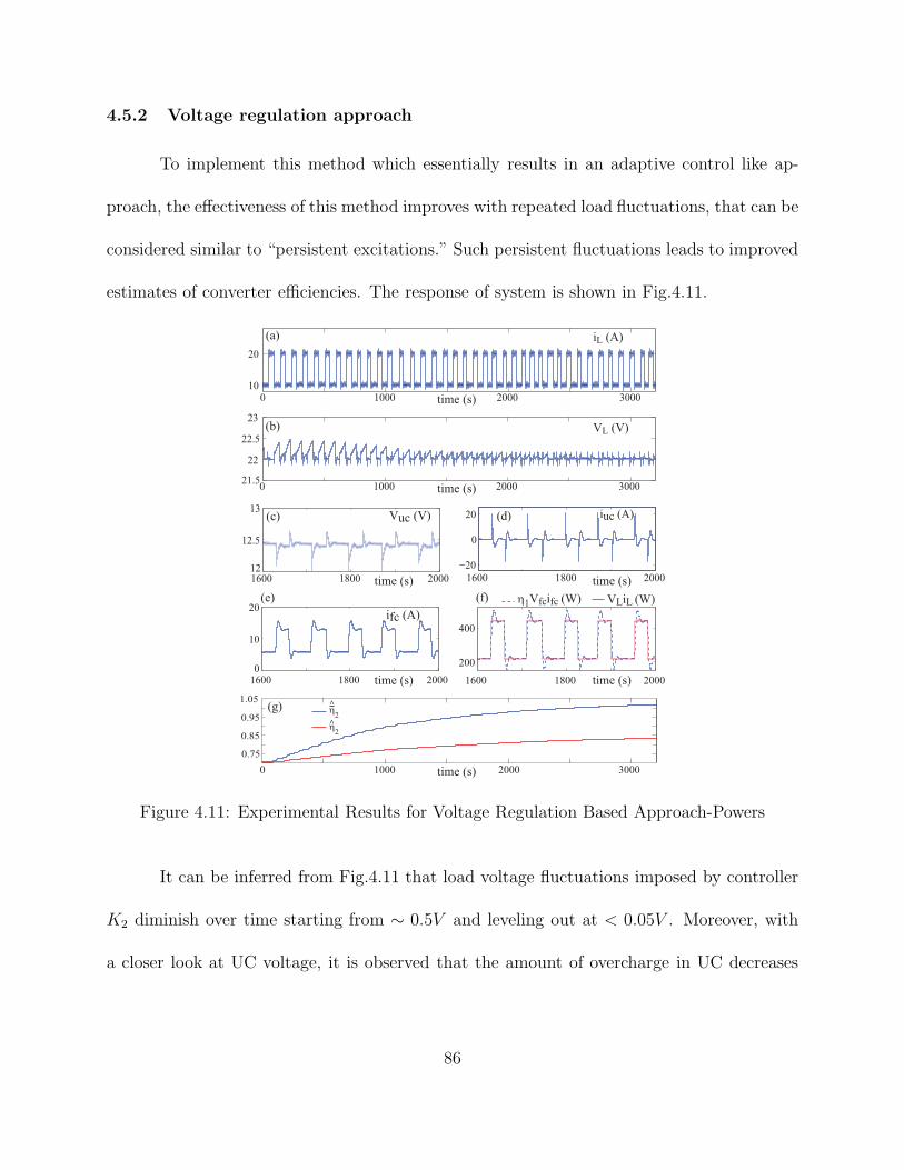
4.5.2 Voltage regulation approach
To implement this method which essentially results in an adaptive control like ap-
proach, the effectiveness of this method improves with repeated load fluctuations, that can be
considered similar to “persistent excitations.” Such persistent fluctuations leads to improved
estimates of converter efficiencies. The response of system is shown in Fig.4.11.
0 1000 2000 3000
22
22.5
23
1600 1800 2000
12.5
13
1600 1800 2000
−20
0
20
1600 1800 2000
10
20
0 1000 2000 300010
20
1600 1800 2000
200
400
3000200010000
0.75
0.85
0.95
1.05
η2
η2
iL (A)
VL (V)
21.5
Vuc (V)
time (s)
time (s)
iuc (A)
time (s)12
time (s)
ifc (A)
time (s) time (s)
η1Vfcifc (W) VLiL (W)
0
time (s)
(a)
(b)
(c) (d)
(e) (f)
(g)
^
^
Figure 4.11: Experimental Results for Voltage Regulation Based Approach-Powers
It can be inferred from Fig.4.11 that load voltage fluctuations imposed by controller
K2 diminish over time starting from ∼ 0.5V and leveling out at < 0.05V . Moreover, with
a closer look at UC voltage, it is observed that the amount of overcharge in UC decreases
86

with time. Moreover, it shows how FC and UC respond to a Load current change. Fig.4.11
also represents how FC provides extra power to make up for energy loss in UC. Overall, it
can be inferred from the curves that the system performance improves over time.
The estimation of η2 and η2 has also been depicted in Fig.4.11. The initial guess
for both of them was set to be η2,min(0) = 0.7. As is visible from the graph, the discharge
efficiency η2 ≃ 0.84, and charge efficiency η2 > 1. It can be seen that the estimation process
is designed such that while η2 is getting estimated, the estimation for η2 is halted, and while
η2 is calculated, the other one is stopped.
4.6 OBSERVATIONS
4.6.1 Overall System Loss Trends
While both approaches described above perform satisfactorily in terms of meeting
the control objectives, they have certain advantages and disadvantages which makes each
approach appealing from different perspectives. The voltage regulation based approach pro-
gressively reduces energy losses; yet it relies on persistent excitation of the load to improve
its efficiency estimates. On the other hand, the dissipation based approach results in uni-
form energy loss, but it does not require perturbations on the network. The energy losses
with each approach were compared and plotted in Fig.4.12. Each data point represents an
average power loss over an interval, calculated as
Wloss,i =1
ti − ti,0
∫ ti
ti,0
(VLiL − Vfcifc) dt (4.18)
87

for both approaches. In Eq.(4.18), ∆ti = ti − ti,0 represents the ith interval ending at ti and
starting at ti,0. Each interval is roughly the same, around 100s, consisting of one step-up
and one step-down in iL. The final instants ti were not all equispaced in time. For example,
(t5 − t4) and (t7 − t6) are longer than the others. It can be observed from the plot that
with voltage regulation, the losses decay over time whereas it is uniform for the dissipation
based approach. The overall magnitudes are not considerably different. This is because the
changes in capacitor voltage due to overcharging (and hence the required dissipation) were
low in our experiments, owing to a high capacity of 250F and comparatively lower power
levels, see Fig.4.10(f). It is expected that with lower capacity storage the advantages of
voltage regulation will be more prominent.
Figure 4.12: Power Loss Trends with Voltage Regulation and Dissipation Approaches
4.6.2 Comparison between Centralized and Decentralized Strategies
As discussed in the Introduction, one advantage of the decentralized approach is fault
tolerance. This is illustrated here for the hybrid SOFC system through a simple observation.
Referring to previous centralized control in [3], the fuel cell current demand ifc,d, which is
88

one control input, was designed as
ifc,d =VLiLη1Vfc
+ g(Es) + δ1(Es) (4.19)
where, Es = S − St, S is the SOC of the ultra-capacitor. The function g and the switching
parameter δ1 are both dependent on Es. However in the decentralized approach proposed in
the paper, ifc,d is designed as given in Eq.(4.7), where the integral Ie is defined in Eq.(4.5). It
is clear from the above two equation that, in centralized case, the control input ifc,d depends
on the SOC, whereas in the latter, the control input is independent of SOC. Therefore, in
the event of a fault in the ultra-capacitor or a fault in sensing the SOC, ifc,d will drive
an incorrect SOFC current demand in the centralized control. This in turn will affect the
SOFC’s fuel flow rate, its delivered power and cause potential depletion or overcharge of
the ultra-capacitor. In contrast, in the decentralized controller the invariance of ifc,d to
SOC will prevent capacitor and thereby system damage. It is however pointed out that the
effectiveness of the decentralized approach over centralized control is also dependent on the
nature of faults. For certain faults the advantage may be clear, while for others secondary
protection will be necessary for both approaches.
4.7 Area Matching Using Dynamic Response of System
In this section, the possibility of implementing a feed forward control scheme using
the same conservation of energy principle discussed in previous chapter will be addressed.
Here, the objective is to come up with a family of solutions for controllers through which
89

the dynamic response of the system will result in a shape for which the summation of areas
above and beneath the load line cancel out each other; i.e. the SOC of the capacitor is
preserved while load is met and fuel utilization of FC is kept within the safe range.
4.7.1 Second Order Under-damped Systems
Referring to Fig.4.2, one could argue that the hybrid system response to step change
in load resembles that of a second order under-damped system. This resemblance motivated
us to investigate weather we can implement the idea of conservation of energy through an
alternative approach. Therefore, we first aimed to obtain the conditions under which the
step response of a second order under-damped system can ensure area matching.
Consider the following second order equation of motion:
X + 2ζωnX + ωn2X = u(t) (4.20)
where 0 ≤ ζ < 1 is the damping ratio and ωn is the natural frequency of the system. The
solution of the above differential equation to a unit step input yields [89],
X(t) =1
ωn2[1− e−σt(cosωdt+
ζ√
1− ζ2sinωdt)] (4.21)
90

where σ = ζωn. Therefore, to implement the method proposed in section 4.3.1, we need to
make sure that the following integral diminishes as time tends toward infinity.
limt→∞
∫ t
0
[X(t)−Xss]dt −→ 0 =⇒ A1 − A2 −→ 0 (4.22)
Applying Eq.(4.21) into Eq.(4.22), and normalize it with respect to steady state response
Xss,
I =
∫∞
0
1
ωn2[−e−σt(cosωdt+
ζ√
1− ζ2sinωdt)] (4.23)
which simplifies into:
− ωn2I =
∫∞
0
e−σt[cosωdt]dt+σ
ωd
∫∞
0
e−σt[sinωdt]dt (4.24)
To ensure the area matching and conservation of energy, Eq.(4.24) needs to be equal to zero.
After simplifying Eq.(4.24) using integral tables, we have:
σ
ωd2 + σ2
+σ
ωd
ωd
ωd2 + σ2
= 0 ⇒ 2ζ
ωn= 0 (4.25)
Eq.(4.25) shows that the only system whose response to a step function can guarantee the
area matching and conservation of energy is a system with no damping. This is quite obvious
as such system has a sinusoidal response to a step function which means the summation of
areas over and under the step will cancel each other out. Therefore, higher order solutions
91

could be sought as an alternative for area matching and conservation of energy method.
Further work in this regards is to be pursued in the future.
4.8 Chapter Summary
A decentralized control approach was developed for a solid oxide fuel cell system
hybridized with an ultra-capacitor in parallel. In the decentralized framework, there are
individual controllers for the fuel cell and the ultra-capacitors that do not explicitly com-
municate with each other but use local information for control. However, the system as a
whole satisfies the control objectives without jeopardizing any component. A conservation
of energy based approach for control was developed. First, a conservative approach was
taken to design the decentralized scheme. This approach was extended to a voltage modu-
lation method which essentially imposed energy conservation on the energy storage device
and simultaneously provided a means for implicit communication between the controllers
using the power line itself. To extend this research in future, a network with more than two
elements and eventually, a network consisting of multiple elements will be attempted. The
general observation is that migrating to a decentralized control involves a trade-off between
the advantage gained through reduced computation and sensing, with the need for adding
a dissipation mechanism or the need for adding an extra capability in power conversion like
voltage modulation.
92

CHAPTER 5CONCLUSIONS
In this work, a method for controlling transient response of the output of a system
for which sensing or accurate estimation was assumed not to be available and comprehensive
information regarding plant was not reachable was proposed. First, the area from where this
problem was raised was described. Then it was shown through both analysis and simulation
that under certain conditions, perfect disturbance attenuation is possible. The method was
then verified in frequency domain as well. Thereafter, the conditions under which transient
control was possible were relaxed and a more general Theorem was expressed and proved. At
the end, the approach were related to fuel cell and similarity and differences were discussed.
It was shown that even though fuel cell system is nonlinear, and time-varying, a linear system
approach can still be applied yielding a reasonable transient response for the output.
Moreover, A decentralized control approach was developed for a solid oxide fuel cell
system hybridized with an ultra-capacitor in parallel. In the decentralized framework, there
are individual controllers for the fuel cell and the ultra-capacitors that do not explicitly
communicate with each other but use local information for control. However, the system as
a whole satisfies the control objectives without jeopardizing any component. A conservation
of energy based approach for control was developed. First, a conservative approach was taken
93

to design the decentralized scheme. This approach was extended to a voltage modulation
method which essentially imposed energy conservation on the energy storage device and
simultaneously provided a means for implicit communication between the controllers using
the power line itself. To extend this research in future, a network with more than two
elements and eventually, a network consisting of multiple elements will be attempted. The
general observation is that migrating to a decentralized control involves a trade-off between
the advantage gained through reduced computation and sensing, with the need for adding
a dissipation mechanism or the need for adding an extra capability in power conversion like
voltage modulation.
Furthermore, The decentralized control framework developed by the authors in [85]
has been further validated using an experimental setup. A few adjustments were made
to the theory to make it compatible based on the practical limitations of our experimental
setup. However, we preserve the main conservation of energy based method for decentralized
control. Moreover, a detailed stability analysis was provided to confirm the performance of
the framework. Both dissipation based and voltage regulation based decentralized controllers
were tested and validated. The notable observation from the experiments was that the
overall system efficiency improves for the voltage regulation approach with time, whereas
the dissipative approach, while being simpler, results in a recurring but limited power loss
in the system. This is an expected phenomena as the voltage regulation method results
in adaptive learning of efficiencies, which over times improves in the presence of repeated
94

fluctuations in load and therefore the conservative approach described in section 4.4.1 evolves
as the exact approach and the over-charging of the ultra-capacitor diminishes over time.
95

LIST OF REFERENCES
[1] T. Das, S. Narayanan, and R. Mukherjee, “Steady-state and transient analysis of asteam-reformer based solid oxide fuel cell system,” Journal of Fuel Cell Science andTechnology, vol. 7, FEB 2010. ASME International Mechanical Engineering Congressand Exposition, Seattle, WA, NOV 11-15, 2007.
[2] T. Allag and T. Das, “Robust nonlinear control of fuel cell ultra-capacitor hybrid sys-tem,” in American Control Conference, pp. 6923–6929, 2010.
[3] T. Allag and T. Das, “Robust control of solid oxide fuel cell ultra-capacitor hybridsystem,” IEEE Transactions on Control Systems Technology, vol. 20, pp. 1–10, January2012.
[4] J. Larminie and A. Dicks, Fuel Cell Systems Explained. John Wiley and Sons Ltd, 2003.
[5] X. Li, Principles of Fuel Cells. Taylor and Francis Group, 2006.
[6] K. Yasuda and T. Ishii, “Basic concept and decentralized autonomous control of super-distributed energy systems,” Electrical Engineering in Japan, vol. 151, no. 1, pp. 43–55,2005.
[7] J. R. Meacham, F. Jabbari, J. Brouwer, J. L. Mauzey, and G. S. Samuelsen, “Analysisof stationary fuel cell dynamic ramping capabilities and ultra capacitor energy storageusing high resolution demand data,” Journal of Power Sources, vol. 156, no. 2, pp. 472– 479, 2006.
[8] T. Das and S. Snyder, “Robust adaptive control of solid oxide fuel cell ultra-capacitorhybrid systems,” IEEE Transactions on Control Systems Technology, vol. 21, no. 2,2013.
[9] R. Gaynor, F. Mueller, F. Jabbari, and J. Brouwer, “On control concepts to prevent fuelstarvation in solid oxide fuel cells,” Journal of Power Sources, vol. 180, pp. 330–342,2008.
[10] A. Drolia, P. Jose, and N. Mohan, “An approach to connect ultracapacitor to fuel cellpowered electric vehicle and emulating fuel cell electrical characteristics using switchedmode converter,” in Industrial Electronics Society, 2003. IECON ’03. The 29th AnnualConference of the IEEE, vol. 1, pp. 897 – 901 vol.1, 2-6 2003.
96

[11] P. Thounthong, S. Rael, and B. Davat, “Control strategy of fuel cell/supercapacitorshybrid power sources for electric vehicle,” Journal of Power Sources, vol. 158, no. 1,pp. 806 – 814, 2006.
[12] A. Vahidi, A. Stefanopoulou, and H. Peng, “Current management in a hybrid fuelcell power system: A model-predictive control approach,” Control Systems Technology,IEEE Transactions on, vol. 14, pp. 1047 –1057, nov. 2006.
[13] F. Mueller, J. Brouwer, F. Jabbari, and S. Samuelsen, “Dynamic simulation of anintegrated solid oxide fuel cell system including current-based fuel flow control,” Journalof Fuel Cell Science and Technology, vol. 3, no. 2, pp. 144–154, 2006.
[14] W. Schmittinger and A. Vahidi, “A review of the main parameters influencing long-termperformance and durability of pem fuel cells,” Journal of Power Sources, vol. 180, no. 1,pp. 1 – 14, 2008.
[15] F. Mueller, F. Jabbari, and J. Brouwer, “On the intrinsic transient capability andlimitations of solid oxide fuel cell systems,” Journal of Power Sources, vol. 187, no. 2,pp. 452 – 460, 2009.
[16] F. Mueller, F. Jabbari, R. Gaynor, and J. Brouwer, “Novel solid oxide fuel cell systemcontroller for rapid load following,” Journal of Power Sources, vol. 172, no. 1, pp. 308– 323, 2007. ACS San Francisco 2006 Fuel and Cell Symposium. American ChemicalSociety National Meeting. San Francisco, CA Sept 10-14 2006.
[17] C. Stiller, B. Thorud, O. Bolland, R. Kandepu, and L. Imsland, “Control strategy for asolid oxide fuel cell and gas turbine hybrid system,” Journal of Power Sources, vol. 158,no. 1, pp. 303–315, 2006.
[18] M. H. Nehrir and C. Wang, Modeling and Control of Fuel Cells - Distributed GenerationApplications. John Wiley and Sons, Inc., 2009.
[19] A. K. M. M. Murshed, B. Huang, and K. Nandakumar, “Estimation and control of solidoxide fuel cell system,” Computers and Chemical Engineering, vol. 34, pp. 96–111, 2010.
[20] S. Campanari, “Thermodynamic model and parametric analysis of a tubular sofc mod-ule,” Journal of Power Sources, vol. 92, no. 1-2, pp. 26 – 34, 2001.
[21] A. Lazzaretto, A. Toffolo, and F. Zanon, “Parameter setting for a tubular sofc simu-lation,” JOURNAL OF ENERGY RESOURCES TECHNOLOGY-TRANSACTIONSOF THE ASME, vol. 126, pp. 40–46, MAR 2004.
[22] K. Sedghisigarchi and A. Felachi, “Control of grid-connected fuel cell power plant fortransient stability enhancement,” Proceedings of the IEEE Power Engineering SocietyTransmission and Distribution Conference, vol. 1, pp. 383–388, January 2002.
97

[23] M. Nayeripour, M. Hoseintabar, and T. Niknam, “A new method for dynamic perfor-mance improvement of a hybrid power system by coordination of converter’s controller,”Journal of Power Sources, vol. 196, no. 8, pp. 4033 – 4043, 2011.
[24] S. A. Hajimolana and M. Soroush, “Dynamics and control of a tubular solid oxide fuelcell,” Industrial & Engineering Chemistry Research, vol. 48, p. 61126125, 2009.
[25] R. Kandepu, L. Imsland, B. A. Foss, C. Stiller, B. Thorud, and O. Bolland, “Mod-eling and control of a sofc-gt-based autonomous power system,” ENERGY, vol. 32,pp. 406–417, APR 2007. 18th International Conference on Efficiency, Costs, Optimiza-tion, Simulation, and Envirinmental Impact of Energy Systems, Trodheim, NORWAY,JUN 22-24, 2005.
[26] A. Reinert and T. Strohbach, “Determination of the global/local fuel utilization viavariation of the fuel utilization,” ECS Transactions, vol. 25, no. 2(1), pp. 811 – 814,2009.
[27] H. Gorgun, M. Arcak, S. Varigonda, and S. A. Bortoff, “Observer designs for fuel pro-cessing reactors in fuel cell power systems,” International Journal of Hydrogen Energy,vol. 30, pp. 447–457, 2005.
[28] J. T. Pukrushpan, A. G. Stefanopoulou, and H. Peng, Control of Fuel Cell PowerSystems: Principles, Modeling, Analysis, and Feedback Design. Advances in IndustrialControl, London: Springer, 2004.
[29] V. Tsourapas, A. G. Stefanopoulou, and J. Sun, “Model-based control of an integratedfuel cell and fuel processor with exhaust heat recirculation,” IEEE Transactions onControl Systems Technology, vol. 15, no. 2, pp. 233–245, 2007.
[30] Y. Guezennec, T. Choi, G. Paganelli, and G. Rizzoni, “Supervisory control of fuel cellvehicles and its link to overall system efficiency and low-level control requirements,” inProceedings of the American Control Conference, pp. 2055–2061, Ohio State University,AACC, June 2003.
[31] M. Grujicic, K. M. Chittajallu, and J. T. Pukrushpan, “Control of the transient be-haviour of polymer electrolyte membrane fuel cell systems,” PROCEEDINGS OF THEINSTITUTION OF MECHANICAL ENGINEERS PART D-JOURNAL OF AUTO-MOBILE ENGINEERING, vol. 218, pp. 1239–1250, NOV 2004.
[32] J. Sun and I. V. Kolmanovsky, “Load governor for fuel cell oxygen starvation protection:a robust nonlinear reference governor approach,” IEEE Transactions on Control SystemsTechnology, vol. 13, pp. 911 – 920, nov. 2005.
[33] C. H. Woo and J. Benziger, “PEM fuel cell current regulation by fuel feed control,”Chemical Engineering Science, vol. 62, no. 4, pp. 957 – 968, 2007.
98

[34] A. Vahidi and W. Greenwell, “A decentralized model predictive control approach topower management of a fuel cell-ultracapacitor hybrid,” in American Control Confer-ence, 2007. ACC ’07, pp. 5431 –5437, july 2007.
[35] A. Arce, A. J. del Real, and C. Bordons, “MPC for battery/fuel cell hybrid vehiclesincluding fuel cell dynamics and battery performance improvement,” Journal of ProcessControl, vol. 19, no. 8, pp. 1289 – 1304, 2009.
[36] S. Espiari and M. Aleyaasin, “Transient response of pem fuel cells during sudden loadchange,” in Energy Conference and Exhibition (EnergyCon), 2010 IEEE International,pp. 211–216, 2010.
[37] D. Bhattacharyya and R. Rengaswamy, “A review of solid oxide fuel cell (SOFC)dynamic models,” Industrial and Engineering Chemistry Research, vol. 48, no. 13,pp. 6068–6086, 2009.
[38] B. Huang, Y. Qi, and M. Murshed, “Solid oxide fuel cell: Perspective of dynamicmodeling and control,” Journal of Process Control, vol. 21, pp. 1426–1437, 2011.
[39] H. Xi, S. Varigonda, and B. Jing, “Dynamic modeling of a solid oxide fuel cell systemfor control design,” in American Control Conference (ACC), 2010, pp. 423–428, June2010.
[40] O. Madani, A. Bhattacharjee, and T. Das, “Decentralized power management in ahybrid fuel cell ultra-capacitor system,” Submitted to IEEE Transactions on ControlSystems Technology, 2014.
[41] A. E. Auld, K. M. Smedley, F. Mueller, J. Brouwer, and G. S. Samuelsen, “Load-following active power filter for a solid oxide fuel cell supported load,” Journal of PowerSources, vol. 195, no. 7, pp. 1905 – 1913, 2010.
[42] P. Thounthong, S. Rael, and B. Davat, “Utilizing fuel cell and supercapacitors forautomotive hybrid electrical system,” in Applied Power Electronics Conference and Ex-position, 2005. APEC 2005. Twentieth Annual IEEE, vol. 1, pp. 90–96 Vol. 1, 2005.
[43] M. Y. Ayad, M. Becherif, A. Djerdir, and A. Miraoui, “Sliding mode control for energymanagement of dc hybrid power sources using fuel cell, batteries and supercapacitors,”in Clean Electrical Power, 2007. ICCEP ’07. International Conference on, pp. 500 –505,21-23 2007.
[44] A. Payman, S. Pierfederici, and F. Meibody-Tabar, “Energy Management in a FuelCell/Supercapacitor Multisource/Multiload Electrical Hybrid System,” IEEE TRANS-ACTIONS ON POWER ELECTRONICS, vol. 24, pp. 2681–2691, DEC 2009.
99

[45] Z. Jiang, L. Gao, and R. A. Dougal, “Adaptive control strategy for active power sharingin hybrid fuel cell/ battery power sources,” IEEE Transactions on Energy Conversion,vol. 22, no. 2, pp. 507–515, 2007.
[46] P. Thounthong, S. Rael, and B. Davat, “Energy management of fuelcell/battery/supercapacitor hybrid power source for vehicle applications,” JOUR-NAL OF POWER SOURCES, vol. 193, pp. 376–385, AUG 1 2009.
[47] V. Paladini, T. Donateo, A. de Risi, and D. Laforgia, “Super-capacitor fuel-cell hybridelectric vehicle optimization and control strategy development,” Energy Conversion andManagement, vol. 48, pp. 3001–3008, 2007.
[48] M. Uzunoglu and M. S. Alam, “Dynamic modeling, design and simulation of a pem fuelcell/ultracapacitor hybrid system for vehicular applications,” Energy Conversion andManagement, vol. 48, pp. 1544–1553, 2007.
[49] A. Hajizadeh and M. A. Golkar, “Intelligent power management strategy of hybrid dis-tributed generation system,” International Journal of Electrical Power, vol. 29, no. 10,pp. 783 – 795, 2007.
[50] T. Das and S. Snyder, “Adaptive control of a solid oxide fuel cell ultra-capacitor hybridsystem,” in American Control Conference (ACC), 2011, pp. 3892 –3898, 29 2011-july 12011.
[51] P. Adhikari and M. Abdelrahman, “Modeling, control, and integration of a portablesolid oxide fuel cell system,” Journal of Fuel Cell Science and Technology, vol. 9, no. 1,p. 011010, 2012.
[52] A. Y. Sendjaja and V. Kariwala, “Decentralized control of solid oxide fuel cells,” Indus-trial Informatics, IEEE Transactions on, vol. 7, no. 2, pp. 163–170, 2011.
[53] L. Bakule, “Decentralized control: An overview,” Annual Reviews in Control, vol. 32,no. 1, pp. 87 – 98, 2008.
[54] M. M. Haddad, Q. Hui, V. Chellaboina, and S. G. Nersesov, “Hybrid decentralized max-imum entropy control for large-scale dynamical systems,” in American Control Confer-ence, 2006, pp. 6 pp.–, 2006.
[55] A. Ramakrishna and N. Viswanadham, “Decentralized control of interconnected dynam-ical systems,” in Decision and Control including the Symposium on Adaptive Processes,1980 19th IEEE Conference on, pp. 538–543, Dec 1980.
[56] Y. Guo, D. J. Hill, and Y. Wang, “Nonlinear decentralized control of large-scale powersystemsq,” Automatica, 2000.
100

[57] V. Ugrinovskii and H. Pota, “Decentralized control of power systems via robust controlof uncertain markov jump parameter systems,” in Proceedings of 43rd IEEE Confer-ence on Decision and Control, pp. 3503–3508, University of New South Wales, IEEE,December 2004.
[58] A. Aquino-Lugo, Distributed and decentralized control of the power grid. PhD thesis,University of Illinois at Urbana-Champaign, 2011.
[59] A. Tuladhar, K. Jin, T. Unger, and K. Mauch, “Parallel operation of single phaseinverter modules with no control interconnections,” in Applied Power Electronics Con-ference and Exposition, 1997. APEC ’97 Conference Proceedings 1997., Twelfth Annual,vol. 1, pp. 94–100 vol.1, Feb 1997.
[60] P. Hines and S. Talukdar, “Reciprocally altruistic agents for the mitigation of cascadingfailures in electrical power networks,” in Infrastructure Systems and Services: Build-ing Networks for a Brighter Future (INFRA), 2008 First International Conference on,pp. 1–6, Nov 2008.
[61] D. Chiappini, A. L. Facci, L. Tribioli, and S. Ubertini, “Sofc management in distributedenergy systems,” Journal of Fuel Cell Science and Technology, vol. 8, no. 3, p. 031015,2011.
[62] A. K. Saha, S. Chowdhury, S. P. Chowdhury, and Y. H. Song, “Application of solid-oxide fuel cell in distributed power generation,” IET Renewable Power Generation,vol. 1, no. 4, pp. 193–202, 2007.
[63] A. Sakhare, A. Davari, and A. Feliachi, “Fuzzy logic control of fuel cell for stand-aloneand grid connection,” Journal of Power Sources, vol. 135, no. 12, pp. 165 – 176, 2004.
[64] M. L. Ferrari, A. Traverso, L. Magistri, and A. F. Massardo, “Influence of the anodicrecirculation transient behaviour on the sofc hybrid system performance,” JOURNALOF POWER SOURCES, vol. 149, pp. 22–32, SEP 26 2005.
[65] F. P. Incropera and D. P. DeWitt, Fundamentals of Heat and Mass Transfer. JohnWiley & Sons, Inc., fifth ed., 2002.
[66] J. Xu and G. F. Froment, “Methane steam reforming, methanation and water-gas shift:I. Intrinsic kinetics,” AIChE Journal, vol. 35, no. 1, pp. 88–96, 1989.
[67] R. Bove, P. Lunghi, and N. M. Sammes, “Sofc mathematic model for systems simula-tions. part one: from a micro-detailed to macro-black-box model,” International Journalof Hydrogen Energy, vol. 30, no. 2, pp. 181 – 187, 2005.
[68] A. Slippey, O. Madani, K. Nishtala, and T. Das, “Invariant properties in solid oxide fuelcell systems with integrated reformers,” Submitted to International Journal of HydrogenEnergy, 2014.
101

[69] T. Bertelsen, T. Pedersen, J. Poulsen, and R. Schultz, “Modelling and optimization ofsolid oxide fuel cell system.” AALBORG University, 2011.
[70] M. J. Kupilik and T. L. Vincent, “Control of a solid oxide fuel cell system with sensitivityto carbon formation,” Journal of Power Sources, vol. 222, no. 0, pp. 267 – 276, 2013.
[71] P. Holtappels, L. Haart, U. Stimming, I. Vinke, and M. Mogensen, “Reaction of co/co2gas mixtures on niysz cermet electrodes,” Journal of Applied Electrochemistry, vol. 29,no. 5, pp. 561–568, 1999.
[72] S. Park, J. M. Vohs, and R. J. Gorte, “Direct oxidation of hydrocarbons in a solid-oxidefuel cell,” Nature (London), vol. 404, pp. 265–267, 2000.
[73] A. Weber, B. Sauer, A. Mller, . Herbstritt, and E. Ivers-Tiffe, “Oxidation of h2, COand methane in SOFCs with ni/ysz-cermet anodes,” Solid State Ionics, vol. 152153,no. 0, pp. 543 – 550, 2002.
[74] B. J. Spivey and T. F. Edgar, “Dynamic modeling, simulation, and MIMO predictivecontrol of a tubular solid oxide fuel cell,” Journal of Process Control, vol. 22, no. 8,pp. 1502 – 1520, 2012. Ken Muske Special Issue.
[75] A. Slippey, “Dynamic modeling and analysis of multiple sofc system configurations,”ms thesis, Rochester Institute of Technology, Rochester, NY, October 2009.
[76] O. Madani and T. Das, “Transient control in multivariable systems: A study motivatedby fuel cells,” in Dynamic systems and control conference (DSCC), 2034, 2013.
[77] J. Klamka, Controllability of dynamical systems. Kluwer Academic Publishers, 1991.
[78] D. Qiu, Q. Wang, and Y. Zhou, “Steady-state output controllability and output control-lability of linear systems,” in Computational Intelligence and Industrial Applications,2009. PACIIA 2009. Asia-Pacific Conference on, vol. 2, pp. 147–150, IEEE, 2009.
[79] W. Jiang, “Output controllability of linear systems with delay,” Journal of Mathematicsfor Technology, vol. 10, pp. 1–6, 1994.
[80] M. I. Garcia-Planas and J. L. Dominguez-Garcia, “Output controllability and steady-output controllability analysis of fixed speed wind turbine,” 2011.
[81] M. D. Brockett, R. W .and Mesarovic, “The reproducibility of multivariable systems,”Journal of mathematical analysis and applications, vol. 11, pp. 548–563, 1965.
[82] M. I. Garcıa-Planas, S. Tarragona, and M. Aplicada, “Analysis of functional output-controllability of time-invariant composite linear systems,” 2013.
[83] D. Bernstein, Matrix Mathematics: Theory, Facts, and Formulas. Princeton universitypress, 2009.
102

[84] S. Skogestad and I. Postlethwaite, Multivariable Feedback Control. Wiley, 1996.
[85] O. Madani and T. Das, “Decentralized control of a fuel cell ultra-capacitor hybridnetwork,” in American Control Conference (ACC), 2013, pp. 5362–5367, 2013.
[86] W. Greenwell and A. Vahidi, “Predictive control of voltage and current in a fuel cell-ultracapacitor hybrid,” IEEE Transactions on Industrial Electronics, vol. 57, pp. 1954–1963, 2010.
[87] A. G. Stefanopoulou and K. Suh, “Mechatronics in fuel cell systems,” Control Engi-neering Practice, vol. 15, pp. 277–289, 2007.
[88] S. Snyder, “Robust adaptive control for a hybrid solid oxide fuel cell system,” Master’sthesis, Rochester Institute of Technology, 2011.
[89] K. Ogata, Modern Control Engineering. Upper Saddle River, NJ, USA: Prentice HallPTR, 4th ed., 2001.
103