Embed Size (px)
Citation preview
Received: 2 May 2016 Revised: 6 September 2016 Accepted: 15 May 2017
DOI: 10.1002/rnc.3862
S H O R T C O M M U N I C A T I O N
Decentralized networked control of discrete-time systems withlocal networks
Dror Freirich Emilia Fridman
School of Electrical Engineering, Tel-Aviv
University, Tel-Aviv, 69978, Israel
CorrespondenceEmilia Fridman, School of Electrical
Engineering, Tel-Aviv University, Tel-Aviv
69978, Israel.
Email: [email protected]
Funding informationIsrael Science Foundation, Grant/Award
Number: 1128/14 ; Kamea Fund of Israel
SummaryThis paper considers discrete-time large-scale networked control systems with mul-
tiple local communication networks connecting sensors, controllers, and actuators.
The local networks operate asynchronously and independently of each other in the
presence of variable sampling intervals, transmission delays, and scheduling pro-
tocols (from sensors to controllers). The time-delay approach that was recently
suggested to decentralized stabilization of large-scale networked systems in the
continuous time is extended to H∞ decentralized control in the discrete time. An
appropriate Lyapunov-Krasovskii method is presented that leads to efficient LMI
conditions for the exponential stability and l2-gain analysis of the closed loop
large-scale system. Differences from the continuous-time results are discussed. A
numerical example of decentralized control of 2 coupled cart-pendulum systems
illustrates the efficiency of the results.
KEYWORDS
decentralized control, large-scale systems, l2-gain, networked control systems, scheduling protocols, time
delay
1 INTRODUCTION
Networked control systems (NCS) are systems with spatially distributed sensors, actuators, and controller nodes, which exchange
data over a communication data channel.1 In the case of large-scale or spatially distributed systems, local groups of sensors and
actuators may be located far apart, leading to a decentralized networked control design. Here, the design may be based on local
controllers and networks.
Decentralized control of continuous-time large-scale systems with independent networks was initiated in Heemels et al2,3 via
the hybrid-system approach. To manage with large communication delays (that may be larger than sampling intervals) in the
presence of scheduling protocols from sensors to actuators, the time-delay approach to continuous-time decentralized NCS was
suggested in Freirich and Fridman.4 The results of Freirich and Fridman4 were confined to stability analysis.
In the discrete-time, stability analysis of large-scale nonlinear systems with application to a power system network was devel-
oped in Gielen and Lazar.5 Self-triggered control of discrete-time systems was studied in Zhang et al.6 The time-delay approach
to discrete-time NCS was developed in Liu and Fridman,7 where the scheduling protocols from sensors to controllers were
considered. The results were confined to the case of 1-plant and 2-sensor nodes.
The goal of this paper is to extend the time-delay approach to decentralized stabilization and H∞ control of large-scale
discrete-time systems with multiple local communication networks connecting sensors, controllers, and actuators. Local net-
works operate asynchronously and independently of each other in the presence of variable sampling intervals, transmission
delays and scheduling protocols from sensors to controllers.
Int J Robust Nonlinear Control. 2018;28:365–380. wileyonlinelibrary.com/journal/rnc Copyright © 2017 John Wiley & Sons, Ltd. 365
366 FREIRICH AND FRIDMAN
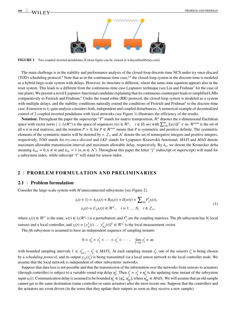
FIGURE 1 Two coupled inverted pendulums [Colour figure can be viewed at wileyonlinelibrary.com]
The main challenge is in the stability and performance analysis of the closed-loop discrete-time NCS under try-once-discard
(TOD) scheduling protocol.8 Note that as in the continuous-time case,4,9 the closed-loop system in the discrete-time is modeled
as a hybrid large-scale system with delays. However, its structure is different, where the same state equation appears also in the
reset system. This leads to a different from the continuous-time case Lyapunov technique (see Liu and Fridman7 for the case of
one plant). We present a novel Lyapunov functional candidate explaining that its continuous counterpart leads to simplified LMIs
comparatively to Freirich and Fridman.4 Under the round robin (RR) protocol, the closed-loop system is modeled as a system
with multiple delays, and the stability conditions naturally extend the conditions of Freirich and Fridman4 to the discrete-time
case. Extension to l2-gain analysis considers both, independent and coupled disturbances. A numerical example of decentralized
control of 2 coupled inverted pendulums with local networks (see Figure 1) illustrates the efficiency of the results.
Notation: Throughout the paper the superscript “T” stands for matrix transposition, n denotes the n dimensional Euclidean
space with vector norm | · |. l2(n) is the space of sequences x(t) ∈ n, t ∈ [0,∞) with∑∞
t=0 ||x(t)||2 < ∞. n×m is the set of
all n × m real matrices, and the notation P > 0, for P ∈ n×n means that P is symmetric and positive definite. The symmetric
elements of the symmetric matrix will be denoted by ∗. + and denote the set of nonnegative integers and positive integers,
respectively. TOD stands for try-once-discard and LKF stands for Lyapunov-Krasovskii functional. MATI and MAD denote
maximum allowable transmission interval and maximum allowable delay, respectively. By 𝛿ij, we denote the Kronecker delta
meaning 𝛿nm = 0, n ≠ m and 𝛿nn = 1 (n,m ∈ ). Throughout this paper the letter “j” (subscript or superscript) will stand for
a subsystem index, while subscript “i” will stand for sensor index.
2 PROBLEM FORMULATION AND PRELIMINARIES
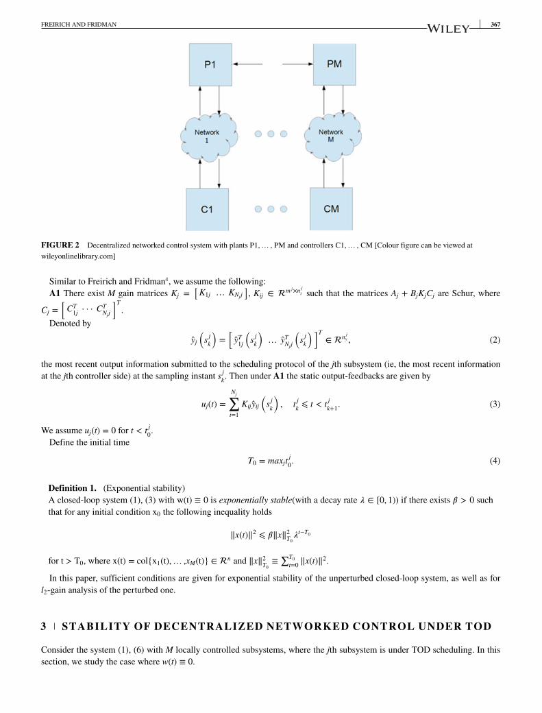
2.1 Problem formulationConsider the large-scale system with M interconnected subsystems (see Figure 2).
xj(t + 1) = Ajxj(t) + Bjuj(t) + Djw(t) +∑
l≠jFl
jxl(t),
yij(t) = Cijxj(t) ∈ n ji , i = 1 … Nj t ∈ +,
(1)
where xj(t) ∈ n jis the state, w(t) ∈ l2(nw) is a perturbation, and Fl
j are the coupling matrices. The jth subsystem has Nj local
sensors and a local controller, and yj(t) = [yT1j(t) … yT
Njj(t)]T ∈ n j
y is the local measurement vector.
The jth subsystem is assumed to have an independent sequence of sampling instants
0 = s j0< s j
1< · · · < s j
k < · · · , limk→∞
s jk = ∞
with bounded sampling intervals 1 ⩽ s jk+1
− s jk ⩽ MATIj. At each sampling instant s j
k, one of the sensors i∗k is being chosen
by a scheduling protocol, and its output yi∗k j(s jk) is being transmitted via a local sensor network to the local controller node. We
assume that the local network is independent of other subsystems' networks.
Suppose that data loss is not possible and that the transmission of the information over the networks from sensors to actuators
(through controller) is subject to a variable round-trip delay 𝜂jk. Then t j
k = s jk + 𝜂
jk is the updating time instant of the subsystem
input uj(t). Communication delay is assumed to be bounded 𝜂jk ∈ [𝜂 j
m, 𝜂jM],where 𝜂
jM ≡ MADj. We will assume that an old sample
cannot get to the same destination (same controller or same actuator) after the most recent one. Suppose that the controllers and
the actuators are event driven (in the sense that they update their outputs as soon as they receive a new sample).
FREIRICH AND FRIDMAN 367
FIGURE 2 Decentralized networked control system with plants P1,… , PM and controllers C1,… , CM [Colour figure can be viewed at
wileyonlinelibrary.com]
Similar to Freirich and Fridman4, we assume the following:
A1 There exist M gain matrices Kj =[
K1j … KNjj], Kij ∈ m j×n j
i such that the matrices Aj + BjKjCj are Schur, where
Cj =[
CT1j · · · CT
Njj
]T.
Denoted by
yj
(s j
k
)=[
yT1j
(s j
k
)… yT
Njj
(s j
k
) ]T∈ n j
y , (2)
the most recent output information submitted to the scheduling protocol of the jth subsystem (ie, the most recent information
at the jth controller side) at the sampling instant s jk. Then under A1 the static output-feedbacks are given by
uj(t) =Nj∑
i=1
Kijyij
(s j
k
), t j
k ⩽ t < t jk+1
. (3)
We assume uj(t) = 0 for t < t j0.
Define the initial time
T0 = maxjt j0. (4)
Definition 1. (Exponential stability)
A closed-loop system (1), (3) with w(t) ≡ 0 is exponentially stable(with a decay rate 𝜆 ∈ [0, 1)) if there exists 𝛽 > 0 such
that for any initial condition x0 the following inequality holds
||x(t)||2 ⩽ 𝛽||x||2T0𝜆t−T0
for t > T0, where x(t) = col{x1(t),… ,xM(t)} ∈ n and ||x||2T0≡∑T0
t=0||x(t)||2.
In this paper, sufficient conditions are given for exponential stability of the unperturbed closed-loop system, as well as for
l2-gain analysis of the perturbed one.
3 STABILITY OF DECENTRALIZED NETWORKED CONTROL UNDER TOD
Consider the system (1), (6) with M locally controlled subsystems, where the jth subsystem is under TOD scheduling. In this
section, we study the case where w(t) ≡ 0.
368 FREIRICH AND FRIDMAN
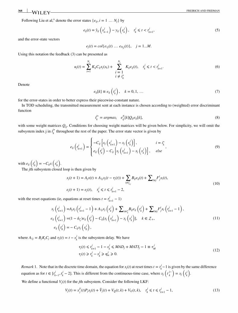
Following Liu et al,9 denote the error states {eij, i = 1 … Nj} by
eij(t) = yij
(s j
k−1
)− yij
(s j
k
), t j
k ⩽ t < t jk+1
, (5)
and the error-state vectors
ej(t) = col{e1j(t) … eNjj(t)}, j = 1...M.
Using this notation the feedback (3) can be presented as
uj(t) =Nj∑
i=1
KijCijxj(sk) +Nj∑
i = 1i ≠ i∗k
Kijeij(t), t jk ⩽ t < t j
k+1. (6)
Denote
eij[k] ≡ eij
(t jk
), k = 0, 1, … (7)
for the error-states in order to better express their piecewise-constant nature.
In TOD scheduling, the transmitted measurement sent at each instance is chosen according to (weighted) error discriminant
function
ij∗k = argmaxi eTij [k]Qijeij[k], (8)
with some weight matrices Qij. Conditions for choosing weight matrices will be given below. For simplicity, we will omit the
subsystem index j in ij∗k throughout the rest of the paper. The error state vector is given by
eij
(t jk+1
)=⎧⎪⎨⎪⎩−Cij
[xj
(s j
k+1
)− xj
(s j
k
)], i = i∗k
eij
(t jk
)− Cij
[xj
(s j
k+1
)− xj
(s j
k
)], else
, (9)
with eij
(t j0
)= −Cijx
(s j
0
).
The jth subsystem closed loop is then given by
xj(t + 1) = Ajx(t) + A1jxj(t − 𝜏j(t)) +∑i≠i∗k,j
Bijeij(t) +∑
l≠jFl
jxl(t),
ej(t + 1) = ej(t), t jk ⩽ t ⩽ t j
k+1− 2,
(10)
with the reset equations (ie, equations at reset times t = t jk+1
− 1)
xj
(t jk+1
)=Ajxj
(t jk+1
− 1)+ A1jxj
(s j
k
)+∑
i≠i∗kBijeij
(t jk
)+∑
l≠jFl
jxl
(t jk+1
− 1),
eij
(t jk+1
)=(1 − 𝛿i∗k )eij
(t jk
)− Cij[xj
(s j
k+1
)− xj
(s j
k
)], k ∈ +,
eij
(t j0
)= − Cijxj
(s j
0
),
(11)
where A1j = BjKjCj and 𝜏j(t) = t − s jk is the subsystem delay. We have
𝜏j(t) ⩽ t jk+1
− 1 − s jk ⩽ MADj + MATIj − 1 ≡ 𝜏
jM
𝜏j(t) ⩾ t jk − s j
k ⩾ 𝜂jm ⩾ 0.
(12)
Remark 1. Note that in the discrete time domain, the equation for xj(t) at reset times t = t jk−1 is given by the same difference
equation as for t ∈ [t jk−1
, t jk − 2]. This is different from the continuous-time case, where xj
(t j−
k
)= xj
(t jk
).
We define a functional Vj(t) for the jth subsystem. Consider the following LKF:
Vj(t) = xTj (t)Pjxj(t) + Vj(t) + VQ(t, k) + VG(t, k), t j
k ⩽ t ⩽ t jk+1
− 1, (13)
FREIRICH AND FRIDMAN 369
where 𝜆 ∈ (0, 1) and
VQ(t, k) = 𝜆t−t jk
Nj∑i=1
eTij (t)Qijeij(t) −
∑i≠i∗k
(t − t j
k
)eT
ij (t)Uijeij(t),
VG(t, k) =t−1∑s=s j
k
Nj∑i=1
𝜆t−s−1zTj (s)C
Tij GijCijzj(s),
Vj(t) = V0j(t) + V1j(t),
V0j(t) =t−1∑
s=t−𝜂 jm
𝜆t−s−1xTj (s)S0jxj(s) + 𝜂
jm
𝜂m∑θ=1
t−1∑s=t−θ
𝜆t−s−1zTj (s)R0jzj(s),
V1j(t) =t−𝜂m−1∑s=t−𝜏 j
M
𝜆t−s−1xTj (s)S1jxj(s) + hj
𝜏j
M∑θ=𝜂 j
m+1
t−1∑s=t−θ
𝜆t−s−1zTj (s)R1jzj(s),
zj(t) = xj(t + 1) − xj(t), hj = (𝜏 jM − 𝜂
jm).
(14)
Here, xTj (t)Pjxj(t) + Vj(t) is a standard LKF for the stability of systems with interval delays,10 VQ(t, k) is constructed to deal with
the error states that appear in (10). The term VG(t, k) allows to compensate the delayed terms Cij[xj
(s j
k+1
)− xj
(s j
k
)] in the
reset (11).
Remark 2. In the continuous-time case, an LKF candidate Vj for the stability analysis of the resulting jth hybrid subsystem
under TOD protocol was suggested in Liu and Fridman9 (for the uncoupled case, where Flj = 0, l ≠ j) and was modified
in Freirich and Fridman4 for coupled (large-scale) systems leading to simplified stability conditions. Thus, the stability of
uncoupled jth subsystem was guaranteed in Freirich and Fridman4 if the following derivative condition holds Vj +2𝛼Vj ⩽ 0
for some 𝛼 > 0 along the continuous-time dynamics, and if Vj does not grow in the reset times. Differently from this, in
the discrete-time case the stability of the uncoupled jth subsystem can be guaranteed if Vj(t + 1) − 𝜆Vj(t) ⩽ 0 with some
𝜆 ∈ (0, 1) for all t (including the reset times t = t jk−1).7 Note that the Lyapunov-Krasovskii method of Liu and Fridman7 was
confined to the case of 2 sensor nodes Nj = 2, and only partial x-stability was established. As in the continuous-time case,4
an extension of results to large-scale systems is not a trivial result that will be presented in Proposition 1 and Theorem 1.
Remark 3. In the discrete-time, by introducing the term VQ(t, k) of (14), we avoid the positive terms containing ||√Qi∗k ei∗k ||2in the upper bound on V(t + 1) − 𝜆V(t) for t ≠ tk − 1. The Qij-terms of VQ in (14) is a discrete-time and modified version of
the corresponding terms in Freirich and Fridman4
VconQ(t) =∑Nj
i=1eT
ij (t)Qi,jeij(t) − 2𝛼(
t − t jk
)eT
i∗k j(t)Qi∗k ,jei∗k j(t),
where the negative term −2𝛼(t jk − t)eT
i∗k j(t)Qi∗k ,jei∗k j(t) allows to compensate a positive term of the form 2𝛼eTi∗k j(t)Qi∗k ,jei∗k j(t) that
arises in Vj(t) + 2𝛼Vj(t).The continuous-time counterpart of Q-terms given by (14) has a form
VcQ(t) = e−2𝛼(t−tk)∑Nj
i=1eT
ij (t)Qi,jeij(t). (15)
The term (15) improves and simplifies the condition for V + 2𝛼V of Freirich and Fridman4 based on VconQ:
VcQ(t) + 2𝛼VcQ(t) = 0 ⩽,
VconQ(t) + 2𝛼VconQ(t) =∑
i≠i∗keT
ij (t)Qi,jeij(t).
However, in the jump condition t = t jk+1
, these functionals lead to different results:
VcQ
(t j+k+1
)− VcQ
(t j−k+1
)=∑Nj
i=1eT
ij
(t jk+1
)Qi,jeij
(t jk+1
)− e−2𝛼
(t jk+1
−t jk
)∑Nj
i=1eT
ij
(t jk
)Qi,jeij
(t jk
),
370 FREIRICH AND FRIDMAN
whereas
VconQ
(t+jk+1
)− VconQ
(t+jk−1
)=∑Nj
i=1eT
ij
(t jk+1
)Qi,jeij
(t jk+1
)−∑Nj
i=1eT
ij
(t jk
)Qi,jeij
(t jk
)+2𝛼(t j
k+1− t j
k)eTij
(t jk
)Qi,jeij
(t jk
)|i=i∗k
.
Hence, VcQ may lead to different from Freirich and Fridman4 (complementary) results. Note that in the example from Freirich
and Fridman4, VcQ does not change the numerical result, but Qi,j terms are eliminated from part of LMIs (simplifying them).
Proposition 1. Consider the jth closed-loop subsystem (10), (11). Given parameters 0 < 𝜆 < 1 and 𝜀 ⩽ 1 − 𝜆(∑
j≠l𝜀jl ⩽𝜀, l = 1 … M) and matrices Pl > 0, l = 1 … M, let there exist matrices S0j,R0j, S1j,R1j,Qij,Uij,Gij > 0, and Wj thatsatisfy LMIs,
Ωj =[
R1j Wj∗ R1j
]⩾ 0 (16)
and
Σ ji − Υ j
i + ETij2GjEij2 < 0,
Ψ ji + [I 0]TUij[I 0] < 0,
i = 1, … ,Nj,
(17)
where
Σ ji = ET
ij1PjEij1 + ETij2HjEij2 − ET
ij3𝜆𝜏
jMΩjEij3 − ET
ij4𝜆𝜂
jm R0jEij4 + Eij5,
hj = 𝜏jM − 𝜂
jm, j = [F1
j · · ·Fl≠jj · · ·FM
j ],Hj = 𝜂j2
m R0j + h2jR1j, Gj =
Nj∑i=1
CTij GijCij,
Eij1 =[Aj
[0 1 0
]⊗ A1j Θij
], Eij2 =
[(Aj − In j
) [0 1 0
]⊗ A1j Θij
], Θij =
[B1j · · ·Br≠ij · · ·BNjj
],
Eij3 =[
02n j×n j
[1 − 1 00 1 − 1
]⊗ In j 0
2n j×(n jy−n j
i )
], Eij4 = [In j − In j 0],
Ei5 = diag{S0j − 𝜆Pj,−(S0j − S1j)𝜆𝜂j
m , 0n j ,−S1j𝜆𝜏
jM , 0},
Ψ ji =
⎡⎢⎢⎢⎣𝜆hjUij +
(1 − Nj𝜆
hj+1
Nj−1
)Qij Qij
∗ Qij − 𝜆𝜏
jM
hj+1Gij
⎤⎥⎥⎥⎦ ,Υ j
i = diag{04n j ,U1j, · · · ,Ur≠i,j, · · · ,UNjj},
Eij1 = [Eij1 j], Eij2 = [Eij2 j], Eij4 = [Eij4 0 · j], Eij3 =[
Eij3 0 ·[ j
j
]],
Eij5 = diag{Eij5,− j}, j = diag{𝜀jlPl, ł ≠ j}, Υ ji = diag{Υ j
i , 0n−nj}.
(18)
Then Vj given by (13) satisfies the following inequalities along (10), (11) (with some 𝛽 j > 0):
Vj(t) ⩾ 𝛽j(||xj(t)||2 + ||ej(t)||2), t ⩾ t j0, (19)
Vj(t + 1) − 𝜆Vj(t) ⩽∑
l≠j𝜀jlxT
l (t)Plxl(t), t ⩾ t j0. (20)
Proof. We prove first the positivity condition 19. Note that
t jk+1
− t jk − 1 = (t j
k+1− 1 − s j
k) − 𝜂jk ⩽ 𝜏
jM − 𝜂
jm = hj. (21)
FREIRICH AND FRIDMAN 371
We have
VQ(t, k) ⩾ 𝜆t jk+1
−1−t jk
Nj∑i=1
eTij (t)Qijeij(t) − (t j
k+1− 1 − t j
k)∑i≠i∗k
eTij (t)Uijeij(t)
⩾ 𝜆hj
Nj∑i=1
eTij (t)Qijeij(t) − hj
∑i≠i∗k
eTij (t)Uijeij(t),
t jk ⩽ t ⩽ t j
k+1− 1.
(22)
From the second inequality (17) it follows that
𝜆hjUij <
[Nj𝜆
hj+1
Nj − 1− 1
]Qij < 𝜆hj+1
[ Nj
Nj − 1− 1
]Qij =
𝜆hj+1
Nj − 1Qij ⩽ 𝜆hj+1Qij.
The latter inequality together with (22) imply
VQ(t, k) ⩾ 𝛽j||ej(t)||2, t jk ⩽ t ⩽ t j
k+1− 1
for some 𝛽 j > 0, yielding (19).
We prove next inequality (20). We find
V0j(t + 1) − 𝜆V0j(t) ⩽ 𝜂j2m zT
j (t)R0jzj(t)
+ xTj (t)S0jxj(t) − 𝜆𝜂
jm xT
j
(t − 𝜂
jm
)S0jxj
(t − 𝜂
jm
)− 𝜂
jm
𝜂j
m∑θ=1
𝜆θzTj (t − θ)R0jzj(t − θ),V1j(t + 1) − 𝜆V1j(t)
⩽ h2j z
Tj (t)R1jzj(t) + 𝜆𝜂
jm xT
j
(t − 𝜂
jm
)S1jxj
(t − 𝜂
jm
)− 𝜆𝜏
jM xT
j
(t − 𝜏
jM
)S1jxj
(t − 𝜏
jM
)− hj
𝜏j
M∑θ=𝜂 j
m+1
𝜆θzTj (t − θ)R1jzj(t − θ).
(23)
By using Jensen's inequality, we obtain
𝜂jm
𝜂j
m∑θ=1
𝜆θzTj (t − θ)R0jzj(t − θ) ⩾ 𝜆𝜂
jm ||√R0j
(xj(t) − xj
(t − 𝜂
jm
)) ||2 =
[𝜂j(t)𝜉ij(t)Xc
j (t)
]T
ETij4𝜆
𝜂j
m R0jEij4
[𝜂j(t)ξij(t)Xc
j (t)
]. (24)
Under (16) the following holds11:
hj
𝜏j
M∑θ=𝜂 j
m+1
𝜆θzTj (t − θ)R1jzj(t − θ) ⩾ 𝜆𝜏
jM
⎡⎢⎢⎣xj
(t − 𝜂
jm
)− xj(t − 𝜏j(t))
xj(t − 𝜏j(t)) − xj
(t − 𝜏
jM
) ⎤⎥⎥⎦T
Ωj
⎡⎢⎢⎣xj
(t − 𝜂
jm
)− xj(t − 𝜏j(t))
xj(t − 𝜏j(t)) − xj
(t − 𝜏
jM
) ⎤⎥⎥⎦=
[𝜂j(t)ξij(t)Xc
j (t)
]T
ETij3𝜆
𝜏j
MΩjEij3
[𝜂j(t)ξij(t)Xc
j (t)
].
(25)
Denote
𝜂j(t) = col{
xj(t), xj
(t − 𝜂
jm
), xj(t − 𝜏j(t)), xj
(t − 𝜏
jM
)}Xc
j (t) = col{xl(t), l ≠ j}, ξij(t) = col{erj(t), r ≠ i},
σij[k] = Cij
(xj
(s j
k+1
)− xj
(s j
k
)).
372 FREIRICH AND FRIDMAN
Employing the relations
zj(t) = Ei∗k j2
⎡⎢⎢⎣𝜂j(t)ξi∗k j(t)Xc
j (t)
⎤⎥⎥⎦ , xj(t + 1) = Ei∗k j1
⎡⎢⎢⎣𝜂j(t)ξi∗k j(t)Xc
j (t)
⎤⎥⎥⎦ (26)
and ∑l≠j𝜀jlxT
l (t)Plxl(t) = XcTj (t) jXc
j (t), (27)
from (23)-(25), we obtain
xTj (t + 1)Pjxj(t + 1) + Vj(t + 1) − 𝜆(xj(t)TPjxj(t) + Vj(t))
−∑
l≠j𝜀jlxT
l (t)Plxl(t) ⩽[𝜂T
j (t) ξTi∗k j(t) XcT
j (t)]Σ j
i∗k
⎡⎢⎢⎣𝜂j(t)ξi∗k j(t)Xc
j (t)
⎤⎥⎥⎦ ,tk ⩽ t ⩽ tk+1 − 1.
(28)
Consider t jk ⩽ t ⩽ t j
k+1− 2. From (21) and definition of VQ(t),
VQ(t + 1, k) − 𝜆VQ(t, k) =(−1 + (𝜆 − 1)
(t − t j
k
))∑i≠i∗k
||√Uijeij(t)||2⩽ −
∑i≠i∗k
||√Uijeij(t)||2 ⩽ −[𝜂T
j (t) ξTi∗k j(t)
]Υ j
i∗k
[𝜂j(t)𝜉i∗k j(t)
]= −
⎡⎢⎢⎣𝜂j(t)ξi∗k j(t)Xc
j (t)
⎤⎥⎥⎦T
Υ ji∗k
⎡⎢⎢⎣𝜂j(t)ξi∗k j(t)Xc
j (t)
⎤⎥⎥⎦ .(29)
Note that the terms |√Qijeij(t)|2 vanish in Equation 29 due to multiplication of them by 𝜆t−t jk .
Therefore,
Vj(t + 1) − 𝜆Vj(t) −∑
l≠j𝜀jlxT
l (t)Plxl(t) ⩽[𝜂T
j (t) ξTi∗k j(t) XcT
j (t)] (
Σ ji∗k− Υ j
i∗k
) ⎡⎢⎢⎣𝜂j(t)ξi∗k j(t)Xc
j (t)
⎤⎥⎥⎦ + zTj (t)Gjzj(t), t j
k ⩽ t ⩽ t jk+1
− 2.
Substituting into the latter inequality 26, we see that the first inequality 17 implies the inequality 20 for t jk ⩽ t ⩽ t j
k+1− 2.
Consider now the case of reset times, where t = t jk+1
− 1. Using notation 7, we have
VQ
(t jk+1
, k + 1)− 𝜆VQ
(t jk+1
− 1, k)
⩽Nj∑
i=1
[eT
ij [k + 1]Qijeij[k + 1] − eTij [k]𝜆
t jk+1
−t jk Qijeij[k]
]+ 𝜆hj
∑i≠i∗k
eTij [k]Uijeij[k].
(30)
Exploiting the reset Equation 9, we find
Nj∑i=1
eTij [k + 1]Qijeij[k + 1] = σT
i∗k j[k]Qi∗k jσTi∗k j[k] +
∑i≠i∗k
(eij[k] + σij[k])TQij(eij[k] + σij[k]). (31)
Since under TOD |√Qi∗k jei∗k j(t)|2 ⩾ 1
Nj − 1
∑i≠i∗k|√Qi,jeij(t)|2, (32)
we arrive atNj∑
i=1
eTij [k]Qijeij[k] = eT
i∗k j[k]Qi∗k jeTi∗k j[k] +
∑i≠i∗k
eij[k]TQijeij[k]
⩾∑i≠i∗k
eij[k]T(
1 + 1
Nj − 1
)Qijeij[k].
(33)
FREIRICH AND FRIDMAN 373
Substituting Equations 31 and 33 into Equation 30 and using Equation 21, we obtain
VQ
(t jk+1
, k + 1)− 𝜆VQ
(t jk+1
− 1, k)
⩽∑i≠i∗k
eTij [k]
[1 − 𝜆hj+1(1 + 1
Nj − 1)]
Qijeij[k] + 𝜆hj∑i≠i∗k
eTij [k]Uijeij[k] + 2
∑i≠i∗k
eTij [k]Qijσij[k]
+∑i≠i∗k
σij[k]TQijσij[k] + σTi∗k j[k]Qi∗k jσT
i∗k j[k].
(34)
For VG, consider 2 cases. In the case, where t = t jk+1
− 1 ⩽ s jk, we have t j
k = s jk, t j
k+1= s j
k+1. Thus,
VG
(t jk+1
, k + 1)− 𝜆VG
(t jk+1
− 1, k)= 0
=Nj∑
i=1
zTj
(t jk+1
− 1)
CTij GijCijzj
(t jk+1
− 1)−
Nj∑i=1
zTj
(s j
k
)CT
ij GijCijzj
(s j
k
)⩽
Nj∑i=1
zTj (t)C
Tij GijCijzj(t) −
𝜆𝜏j
M
hj + 1
Nj∑i=1
σTij [k]Gijσij[k].
(35)
Here, the latter inequality is due to Jensen's inequality.
Otherwise, t jk+1
− 1 > s jk, and similarly to Equation 35, we have
VG
(t jk+1
, k + 1)− 𝜆VG
(t jk+1
− 1, k)
⩽Nj∑
i=1
zTj
(t jk+1
− 1)
CTij GijCijzj
(t jk+1
− 1)−
s jk+1
−1∑s=s j
k
Nj∑i=1
𝜆t jk+1
−s−1zTj (s)C
Tij GijCijzj(s)
⩽Nj∑
i=1
zTj (t)C
Tij GijCijzj(t) −
𝜆𝜏j
M
hj + 1
Nj∑i=1
σTij [k]Gijσij[k].
(36)
Summarizing, we obtain
VQ
(t jk+1
, k + 1)+ VG
(t jk+1
, k + 1)− 𝜆(VQ
(t jk+1
− 1, k)+ VG
(t jk+1
− 1, k))
⩽ zj(t)TGjzj(t) +∑i≠i∗k
[eij[k]σij[k]
]T
Ψ ji
[eij[k]σij[k]
]+[
ei∗k j[k]σi∗k j[k]
]T(
Qi∗k j −𝜆𝜏
jM
hj + 1Gi∗k j
)[ei∗k j[k]σi∗k j[k]
],
(37)
and together with Equation 28
Vj
(t jk+1
)− 𝜆Vj
(t jk+1
− 1)−∑
l≠j𝜀jl||√Plxl(tk+1 − 1)||2
⩽[𝜂T
j (t) ξTi∗k j(t) XcT
j (t)]Σ j
i∗k
⎡⎢⎢⎣𝜂j(t)ξi∗k j(t)Xc
j (t)
⎤⎥⎥⎦ + zj(t)TGjzj(t)
+∑i≠i∗k
[eij[k]σij[k]
]T
Ψ ji
[eij[k]σij[k]
]+[
ei∗k j[k]σi∗k j[k]
]T(
Qi∗k j −𝜆𝜏
jM
hj + 1Gi∗k j
)[ei∗k j[k]σi∗k j[k]
].
(38)
From the second inequality (Equation 17), it follows that
Qi∗k j −𝜆𝜏
jM
hj + 1Gi∗k j < 0.
374 FREIRICH AND FRIDMAN
Therefore,
Vj
(t jk+1
)− 𝜆Vj
(t jk+1
− 1)−∑
l≠j𝜀jl||√Plxl(tk+1 − 1)||2
⩽[𝜂T
j (t) ξTi∗k j(t) XcT
j (t)]Σ j
i∗k
⎡⎢⎢⎣𝜂j(t)ξi∗k j(t)Xc
j (t)
⎤⎥⎥⎦ + zj(t)TGjzj(t) +∑i≠i∗k
[eij[k]σij[k]
]T
Ψ ji
[eij[k]σij[k]
].
(39)
Note that
[𝜂T
j (t) ξTi∗k j(t) XcT
j (t)]Υ j
i∗k
⎡⎢⎢⎣𝜂j(t)ξi∗k j(t)Xc
j (t)
⎤⎥⎥⎦ −∑i≠i∗k
eTij [k]Uijeij[k] = 0. (40)
So, by adding Equation 40 to Equation 39, we arrive at
Vj
(t jk+1
)− 𝜆Vj
(t jk+1
− 1)−∑
l≠j𝜀jl||√Plxl(tk+1 − 1)||2 ⩽
[𝜂T
j (t) ξTi∗k j(t) XcT
j (t)] (
Σ ji∗k− Υ j
i∗k
) ⎡⎢⎢⎣𝜂j(t)ξi∗k j(t)Xc
j (t)
⎤⎥⎥⎦ + zj(t)TGjzj(t)
+∑i≠i∗k
[eij[k]σij[k]
]T
Ψ ji
[eij[k]σij[k]
]+∑i≠i∗k
eTij [k]Uijeij[k].
(41)
Hence, taking into account Equation 26, the inequality 17 implies Equation 20 for t = t jk+1
− 1.
We are in a position to formulate the stability result.
Theorem 1. Consider the large-scale system (Equations 10 and 11), j = 1 … M. Given tuning parameters 0 < 𝜆 < 1
and 𝜀 ⩽ 1 − 𝜆(∑
j≠l𝜀jl ⩽ 𝜀, l = 1 … M), let there exist matrices Pj, S0j,R0j, S1j,R1j,Qij,Uij,Gij > 0, and Wj that satisfyEquations 16 and 17 for all j = 1 … M. Then the system (Equations 10 and 11) is exponentially stable with a decay rate𝜆 + 𝜀.
Proof. From Proposition 1, Equations 16 and 17 imply the inequality 19 for j = 1 … M. Then there exist positive {𝛽j}Mj=1
such that
Vj(t) ⩾ xTj (t)Pjxj(t) + 𝛽j||ej(t)||2. (42)
Consider now the LKF
V(t) =M∑
j=1
Vj(t). (43)
Since xTj (t)Pjxj(t) ⩽ Vj(t) and
∑j≠l𝜀jl ⩽ 𝜀, l = 1 … M, summing Equation 20 over j = 1 … M for t ⩾ T0, we obtain
V(t + 1) − (𝜆 + 𝜀)V(t) ⩽ 0
that implies
V(t) ⩽ (𝜆 + 𝜀)t−T0 V(T0), t > T0. (44)
Inequalities (Equation 20) for j = 1...M yield
Vj(T0) ⩽ 𝜆T0−t j0 Vj
(t j0
)+
T0∑s=t j
0
∑l≠j
𝜆T0−s𝜀jlxTl (t)Plxl(t).
FREIRICH AND FRIDMAN 375
Then there exist some constants Cj such that
Vj(T0) ⩽ Vj
(t j0
)+ 1
2Cj||x||2T0
⩽ Cj||x||2T0,∀j.
Hence, for some constant C, we have
V(T0) ⩽ C||x||2T0,
implying (for some 𝛽− > 0)
𝛽−(||x(t)||2 + M∑j=1
||ej(t)||2) ⩽ V(t) ⩽ C||x||2T0(𝜆 + 𝜀)(t−T0)
with 𝜆 + 𝜀 < 1.
Remark 4. Note that differently from Freirich and Fridman,4 the LMIs (Equation 17) are not affine in the system matrices.
This is due to substitution of Equation 26 into the positive terms zTj (t)HjzT
j (t), zTj (t)GjzT
j (t), and xTj (t + 1)Pjxj(t + 1) of
Vj(t + 1) − 𝜆Vj(t). However, by applying Schur complements to these terms, one can arrive at equivalent to Equation 17
LMIs that are affine in the systems matrices. Hence, the result of Theorem 1 is applicable to the case of system matrices
from an uncertain time-varying polytope, where one can solve the LMIs (Equation 17) simultaneously for all the vertices
of the polytope applying the same decision matrices.
4 L2-GAIN ANALYSIS OF THE LARGE-SCALE SYSTEM
Consider now the large-scale system (Equation 1) under the controller (Equation 6), where all subsystems are orchestrated by
TOD protocol. The closed loop is then given by
xj(t + 1) = Ajx(t) + A1jxj(t − 𝜏j(t)) +∑i≠i∗k,j
Bijeij[k] +∑
l≠jFl
jxl(t) + Djwj(t), t jk ⩽ t ⩽ t j
k+1− 1, j = 1 … M,
(45)
where w(t) = col{wj(t), j = 1 … M} ∈ l2([T0,∞),Rnw) is a disturbance. Let Z(t) = col{Zj(t), j = 1 … M} be the controlled
output, where
Zj(t)= 𝛬1jxj(t)+𝛬2juj(t) ∈ nz .
Given 𝛾 > 0, define the following performance index
J =∞∑
t=t0
[∑j
ZTj (t)Zj(t) − γ2wT (t)w(t)
].
Definition 2. The closed-loop large-scale system (Equation 45) with initial time T0 = maxj{t j0} is said to have an induced
l2-gain less than 𝛾 , if
J < V(T0), ∀w ∈ l2(nw), w ≠ 0
holds for V given by Equation 43.
It is well known (see, eg, Fridman10) that J < V(T0) if for some 𝛼 > 0, the following condition holds along Equation 45
V(t + 1) − V(t) + ZT (t)Z(t) − γ2wT (t)w(t) ⩽ −α[||x(t)||2 + ||w(t)||2], t ⩾ T0. (46)
376 FREIRICH AND FRIDMAN
Lemma 1. Consider {Vj(t)}Mj=1
given by Equation 13. Let there exist positive tuning parameters 𝜀 < 1 and {𝜀jl}Mj,l=1
suchthat
∑j≠l𝜀jl ⩽ 𝜀, l = 1 … M and
Vj(t + 1) − (1 − 𝜀)Vj(t) + ZTj (t)Zj(t) − 𝛾2wT
j (t)wj(t) ⩽∑
l≠j𝜀jlxT
l (t)Plxl(t) (47)
for t ⩾ T0, then Equation 46 holds along Equation 45 with V(t) =∑M
j=1 Vj(t).
Taking into account Equation 42, the result of Lemma 1 follows from summation in Equation 47. By extending derivations
of Proposition 1, we arrive at the following LMI conditions that guarantee Equation 47.
Theorem 2. Given 𝛾 > 0, consider the closed-loop system (Equation 45) with a tuning parameter 0 < 𝜀 < 1(∑
j≠l𝜀jl ⩽𝜀, l = 1 … M). Let there exist matrices Pj, S0j,R0j, S1j,R1j,Qij,Uij,Gij > 0 and Wj such that Equation 16 holds for allj = 1 … M, and
Σ ji − Υ j
i + ETij2GjEij2 + 𝜁T
ij 𝜁ij < 0,Ψ ji + [I 0]TUij[I 0] < 0,
i = 1, … ,Nj, j = 1, … ,M,(48)
where 𝜆 = 1 − 𝜀 and
Σ ji = ET
ij1PjEij1 + ETij2HjEij2 − ET
ij3𝜆𝜏MΩjEij3 − ET
ij4𝜆𝜂
jm R0jEij4 + Eij5,
hj = 𝜏jM − 𝜂
jm, j = [F1
j · · ·Fl≠jj · · ·FM
j ],
Eij1 = [Eij1 j Dj], Eij2 = [Eij2 j Dj],
Eij4 = [Eij4 0 · j 0 · Dj], Eij3 =[
Eij3 0 ·[ j Dj j Dj
]],
Eij5 = diag{Eij5,− j,−𝛾2In jw}, j = diag{𝜀jlPl≠j},
Υ ji = diag{Υ j
i , 0n−nj , 0n jw},
ji = row{Krj, r ≠ i}
𝜁ij = [𝛬1j [0 1 0]⊗𝛬2jKjCj 𝛬2jji 0]
(49)
with notations given by Equation 18. Then the large-scale system (Equation 45) has an induced l2-gain less than 𝛾 , whereV(t) =
∑jVj(t) and Vj(t) are given by Equation 13.
Remark 5. In the general case where disturbance is common for all subsystems (ie, wj(t) ≡ w(t), j = 1 … M), we modify
condition 47 as
Vj(t + 1) − (1 − 𝜀)Vj(t) + ZTj (t)Zj(t) − wT (t)Γjw(t) ⩽
∑l≠j𝜀jlxT
l (t)Plxl(t),
where nw × nw positive definite matrices 𝛤j are subject to 𝛾2Inw ⩾∑
jΓj. Then Theorem 2 still holds if for every j, 𝛾2In j
w
in Equation 49 is replaced by 𝛤j. Here, {Γj}Mj=1
are additional decision variables of LMIs. The resulting bound 𝛾Rem on
the l2-gain is given by 𝛾2Rem = 𝛾2
Rem(Γj) = 𝛾2. Simpler LMIs, where 𝛾2In jw
in Equation 49 is replaced by (common for all
j)𝛾2Inw∕M may lead to a larger bound 𝛾2Rem = 𝛾2
Rem(𝛾) = 𝛾2 (as shown in the example below).
5 ABOUT DECENTRALIZED CONTROL UNDER RR PROTOCOL
Consider next stabilization of Equation 1 (wj = 0), where RR scheduling protocol orchestrates the transmitted measurements
sent at each instance from sensors to a controller for every subsystem. Under RR scheduling, transmitted sensor measurement
is chosen in a periodic manner. In this case the control law (6) can be presented as
uj(t) =Nj∑
i=1
KijCijxj(t − 𝜏j(t)),
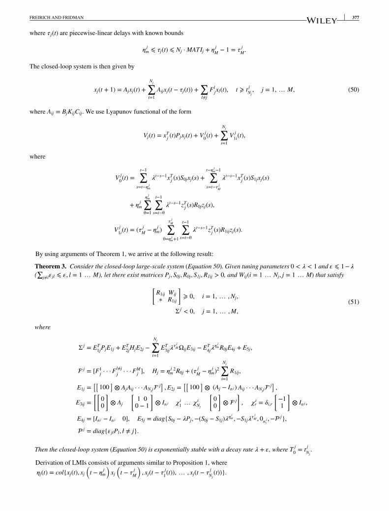
FREIRICH AND FRIDMAN 377
where 𝜏 j(t) are piecewise-linear delays with known bounds
𝜂jm ⩽ 𝜏j(t) ⩽ Nj · MATIj + 𝜂
jM − 1 = 𝜏
jM .
The closed-loop system is then given by
xj(t + 1) = Ajxj(t) +Nj∑
i=1
Aijxj(t − 𝜏j(t)) +∑l≠j
Fljxl(t), t ⩾ t j
Nj, j = 1, … M, (50)
where Aij = BjKijCij. We use Lyapunov functional of the form
Vj(t) = xTj (t)Pjxj(t) + V j
0(t) +
Nj∑i=1
V j1i(t),
where
V j0(t) =
t−1∑s=t−𝜂 j
m
𝜆t−s−1xTj (s)S0jxj(s) +
t−𝜂 jm−1∑
s=t−𝜏 jM
𝜆t−s−1xTj (s)S1jxj(s)
+ 𝜂jm
𝜂j
m∑θ=1
t−1∑s=t−θ
𝜆t−s−1zTj (s)R0jzj(s),
V j1i(t) = (𝜏 j
M − 𝜂jm)
𝜏j
M∑θ=𝜂 j
m+1
t−1∑s=t−θ
𝜆t−s−1zTj (s)R1ijzj(s).
By using arguments of Theorem 1, we arrive at the following result:
Theorem 3. Consider the closed-loop large-scale system (Equation 50). Given tuning parameters 0 < 𝜆 < 1 and 𝜀 ⩽ 1−𝜆
(∑
j≠l𝜀jl ⩽ 𝜀, l = 1 … M), let there exist matrices Pj, S0j,R0j, S1j,R1ij > 0, and Wij(i = 1 … Nj, j = 1 … M) that satisfy[R1ij Wij∗ R1ij
]⩾ 0, i = 1, … ,Nj,
Σ j < 0, j = 1, … ,M,
(51)
where
Σ j = ET1jPjE1j + ET
2jHjE2j −Nj∑
i=1
ET3ij𝜆
𝜏j
MΩijE3ij − ET4j𝜆
𝜂j
m R0jE4j + E5j,
j = [F1j · · ·F
l≠jj · · ·FM
j ], Hj = 𝜂jm
2R0j + (𝜏 jM − 𝜂
jm)2
Nj∑i=1
R1ij,
E1j =[[
100]⊗ AjAij · · ·ANjj
j] ,E2j =[[
100]⊗ (Aj − In j ) Aij · · ·ANjj
j] ,E3ij =
[[00
]⊗ Aj
[1 0
0 − 1
]⊗ In j 𝜒 i
1… 𝜒 i
Nj
[00
]⊗ j
], 𝜒 i
r = 𝛿i,r
[−11
]⊗ In j ,
E4j = [In j − In j 0], E5j = diag{S0j − 𝜆Pj,−(S0j − S1j)𝜆𝜂j
m ,−S1j𝜆𝜏
jM , 0n j
y,− j},
j = diag{𝜀jlPl, ł ≠ j}.
Then the closed-loop system (Equation 50) is exponentially stable with a decay rate 𝜆 + 𝜀, where T j0= t j
Nj.
Derivation of LMIs consists of arguments similar to Proposition 1, where
𝜂j(t) = col{xj(t), xj
(t − 𝜂
jm
)xj
(t − 𝜏
jM
), xj(t − 𝜏
j1(t)), … , xj(t − 𝜏
jNj(t))}.
378 FREIRICH AND FRIDMAN
Remark 6. In the numerical example below, the results that follow from Theorem 3 (under RR protocol) are less conservative
than the results based on Theorem 1. However, the improvement is achieved on the account of the numerical complexity:
• the conditions of Theorem 1 possess LMIs of Njn + (4Nj + 7)nj + 4njy total rows and
5Tn j + nj2 + 3∑Nj
i=1Tn j
iscalar decision variables for each subsystem j, where Tn = n2+n
2is the nth triangular number;
• the conditions of Theorem 3 possess LMIs of (6 + 4Nj)nj + n total rows and
(4 + Nj)Tn j + Njn j2 scalar decision variables for each subsystem j.
Comparatively to LMIs of Theorem 1, the number of lines in LMIs of Theorem 2 is enlarged by Njn jw, whereas the number
of scalar decision variables remains the same.
Remark 7. There is a trade-off between enlarging the decay rate and the values of MATI/MAD. The choice of a decay rate
𝜆 close to 1 enlarges the values of MATI/MAD. Moreover, fast convergence of subsystems without coupling, where 𝜆 ≪ 1
if Flj = 0, allows stronger coupling.
6 EXAMPLE: 2 COUPLED INVERTED PENDULUMS
Consider the example of 2 coupled inverted pendulums on carts (Figure 1), under the scenario of decentralized networked
control. We discretize the continuous-time model of Borgers and Heemels2 with the sampling time Ts = 10−4. Here M = 2,
Nj = 2 or Nj = 4(j = 1, 2). The resulting system matrices of Equations 1 and 3 are given by
Aj = A = I4 + 10−4 ·⎡⎢⎢⎢⎣
0 1 0 02.9156 0 −0.0005 0
0 0 0 1−1.6663 0 0.0002 0
⎤⎥⎥⎥⎦ ,BT
j = BT = 10−4 ·[
0 − 0.0042 0 0.0167],
F21= F1
2= A12 = 10−4 ·
⎡⎢⎢⎢⎣0 0 0 0
0.0011 0 0.0005 00 0 0 0
−0.0003 0 −0.0002 0
⎤⎥⎥⎥⎦ ,K1 = [k11 k21 k31 k41] = [11396 7196.2 573.96 1199.0] ,K2 = [k12 k22 k32 k42] = [29241 18135 2875.3 3693.9] .
In the case of Nj = 2, we consider
C1j =[
1 0 0 00 1 0 0
], C2j =
[0 0 1 00 0 0 1
],
K1j = [k1j k2j], K2j = [k3j k4j], j = 1, 2.
In the case of Nj = 4, C1j, … ,C4j are the rows of I4 and K1j, … ,K4j are the entries of Kj.
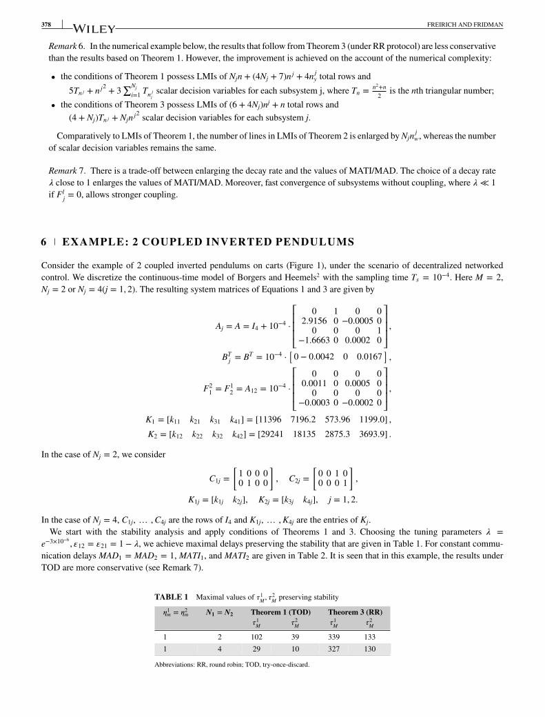
We start with the stability analysis and apply conditions of Theorems 1 and 3. Choosing the tuning parameters 𝜆 =e−3×10⁻⁶
, 𝜀12 = 𝜀21 = 1 − 𝜆, we achieve maximal delays preserving the stability that are given in Table 1. For constant commu-
nication delays MAD1 = MAD2 = 1, MATI1, and MATI2 are given in Table 2. It is seen that in this example, the results under
TOD are more conservative (see Remark 7).
TABLE 1 Maximal values of 𝜏1M , 𝜏2
M preserving stability
𝜂1m = 𝜂2
m N1 = N2 Theorem 1 (TOD) Theorem 3 (RR)𝜏1
M 𝜏2M 𝜏1
M 𝜏2M
1 2 102 39 339 133
1 4 29 10 327 130
Abbreviations: RR, round robin; TOD, try-once-discard.
FREIRICH AND FRIDMAN 379
TABLE 2 MATI1,MATI2 preserving stability for MAD = 1
𝜂1m = 𝜂2
m N1 = N2 Theorem 1 (TOD) Theorem 3 (RR)MATI1 MATI2 MATI1 MATI2
1 2 101 38 169 66
1 4 28 9 81 32
Abbreviations: RR, round robin; TOD, try-once-discard.
TABLE 3 Results of Freirich and Fridman4: max. value of 𝜏j
M preserving
stability ( j = 1, 2) for 𝜂1m = 𝜂2
m = 10−4
#Sensors(Nj) 2 4𝜏1
M 𝜏2M 𝜏1
M 𝜏2M
Freirich and Fridman4 (TOD) 0.0103 0.004 0.003 0.001
Abbreviation: TOD, try-once-discard.
TABLE 4 Minimal values of γ2Rem
N1 = N2 𝜂1m = 𝜂2
m 𝜏1M 𝜏2
M γ2Rem(Γj) γ2
Rem(γ)
2 1 2 2 0.0262 0.0482
4 1 2 2 0.0461 0.0791
Table 3 illustrates that in this example under TOD, the discrete-time results with Ts = 10−4 are similar to the continuous-time
ones obtained in Freirich and Fridman.4 The same is true for the results under RR.
Consider now the perturbed model of 2 coupled inverted pendulums given as above, where each system input is perturbed
such that
uj(t) = uj(t) + 𝜈j(t) +9
10𝜈3−j(t), j = 1, 2.
Here, uj(t) are the controllers as considered above, and 𝜈1 and 𝜈2 ∈ l2 are the perturbations. The system is now given by
Equation 45 where wT1(t) = wT
2(t) =
[𝜈T
1(t) 𝜈T
2(t)]
and
D1 =[
B19
10B1
], D2 =
[9
10B2 B2
].
The controlled output is given by
Z1(t) = [500 0 0 0] · x1(t), Z2(t) = [100 0 0 0] · x2(t).
Choosing 𝜆, 𝜀12, and 𝜀21 as above, we find bounds on l2-gain by using Remark 5 with different 𝛤j, denoted by 𝛾Rem(𝛤j), and
common 𝛾2Inw∕M, denoted by 𝛾Rem(𝛾), (see Table 4). Here, for Nj = 2, the following gain matrices are obtained:
Γ1 = diag{0.0224, 0.0216}, Γ2 = diag{0.0038, 0.0045},
and for Nj = 4,
Γ1 = diag{0.04, 0.0388}, Γ2 = diag{0.0061, 0.0073}.
It is seen that the bounds on 𝛾Rem achieved by using different 𝛤j are less restrictive. However, the corresponding LMIs possess
more decision variables.
7 CONCLUSIONS
In this paper, a time-delay approach has been developed for the decentralized networked control of large-scale discrete-time sys-
tems with local networks, where asynchronous variable sampling intervals, large variable communication delays and scheduling
protocols from sensors to controllers were taken into account. The proposed Lyapunov-Krasovskii method leads to efficient
LMI conditions for the exponential stability and l2-gain analysis of the closed-loop large-scale system.

380 FREIRICH AND FRIDMAN
ACKNOWLEDGEMENTSThis work was partially supported by Israel Science Foundation (grant no 1128/14) and by Kamea Fund of Israel.
REFERENCES1. Antsaklis P, Baillieul J. Special issue on technology of networked control systems. Proc IEEE. 2007;95(1):5-8.
2. Borgers D, Heemels WPMH. Stability analysis of large-scale networked control systems with local networks: a hybrid small-gain approach. CSTreport. 2014.
3. Heemels WPMH, Borgers D, van de Wouw N, Nesic D, Teel A. Stability analysis of nonlinear networked control systems with asynchronous
communication: a small-gain approach. In Proceedings of the 52th IEEE Conference on Decision and Control. Florence; 2013:4631-4637.
4. Freirich D, Fridman E. Decentralized networked control of systems with local networks: a time-delay approach. Autom. 2016;69:201-209.
5. Gielen RH, Lazar M. On stability analysis methods for large-scale discrete-time systems. Autom. 2015;55:66-72.
6. Zhang J, Zhao D, Zheng WX. Output feedback control of discrete-time systems with self-triggered controllers. Int J Robust Nonlinear Control.2015;25(18):3698-3713.
7. Liu K, Fridman E. Discrete-time network-based control under scheduling and actuator constraints. Int J Robust Nonlinear Control.2015;25:1816-1830.
8. Walsh GC, Beldiman O, Bushnell LG. Asymptotic behavior of nonlinear networked control systems. IEEE Trans Autom Control. 2001;46(7):
1093-1097.
9. Liu K, Fridman E, Hetel L. Networked control systems in the presence of scheduling protocols and communication delays. SIAM J ControlOptim. 2015;53(4):1768-1788.
10. Fridman E. Introduction to time-delay systems: analysis and control, Birkhauser, Systems and Control: Foundations and Applications. Basel;
2014.
11. Park PG, Ko J, Jeong C. Reciprocally convex approach to stability of systems with time-varying delays. Autom. 2011;47:235-238.
How to cite this article: Freirich D, Fridman E. Decentralized networked control of discrete-time systems with local
networks. Int J Robust Nonlinear Control. 2018;28:365–380. https://doi.org/10.1002/rnc.3862