Embed Size (px)
Citation preview

Decentralized Dynamics for Finite Opinion Games
Diodato Ferraioli, LAMSADEPaul Goldberg, University of LiverpoolCarmine Ventre, Teesside University

Opinion Formation in SAGT12 social network*
* All characters appearing in this talk are fictitious. Any resemblance to real persons, living or dead, is purely coincidental.
…
…
…
Should carbonara have cream?
Y N
…
…
…
Y
Y
Y NYN
(Aside note: The right answer is NO!)

PREVIOUS WORK
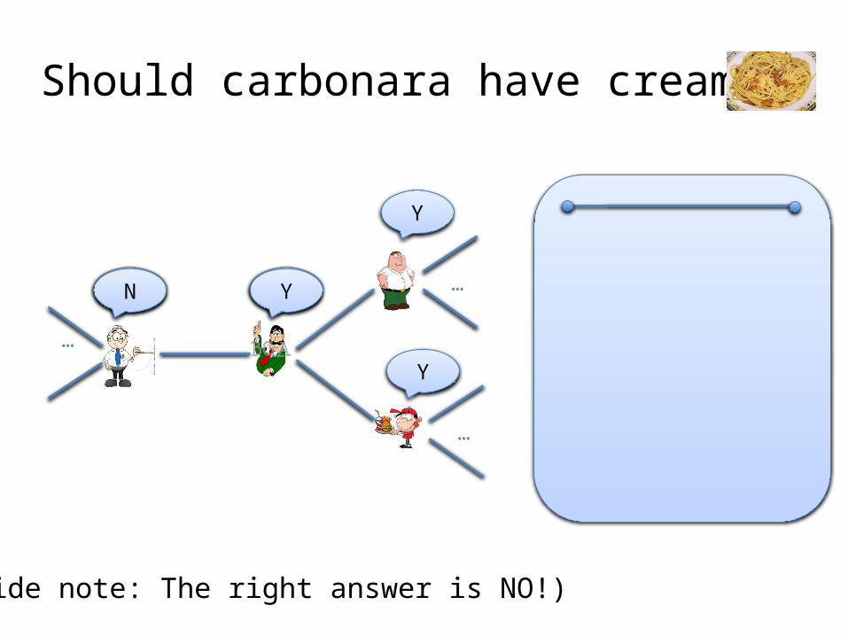
Repeated averaging: De Groot’s model
…
…
…1
.50 1
.3
0
.45
.46
.23
.36
Econ question: Under what conditions repeated averaging leads to consensus?
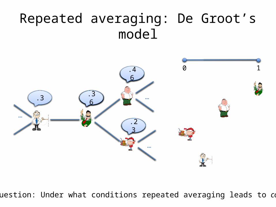
Friedkin and Johnsen’s variation of De Groot’s model [Bindel, Kleinberg & Oren, FOCS 2011 ]
…
…
…
1
.5
.3
0
.45
.46
.23
.5
0 1
Note: It is (0.23+0.3+0.46+1)/4 ≈ 0.5 (≠ 0.36)
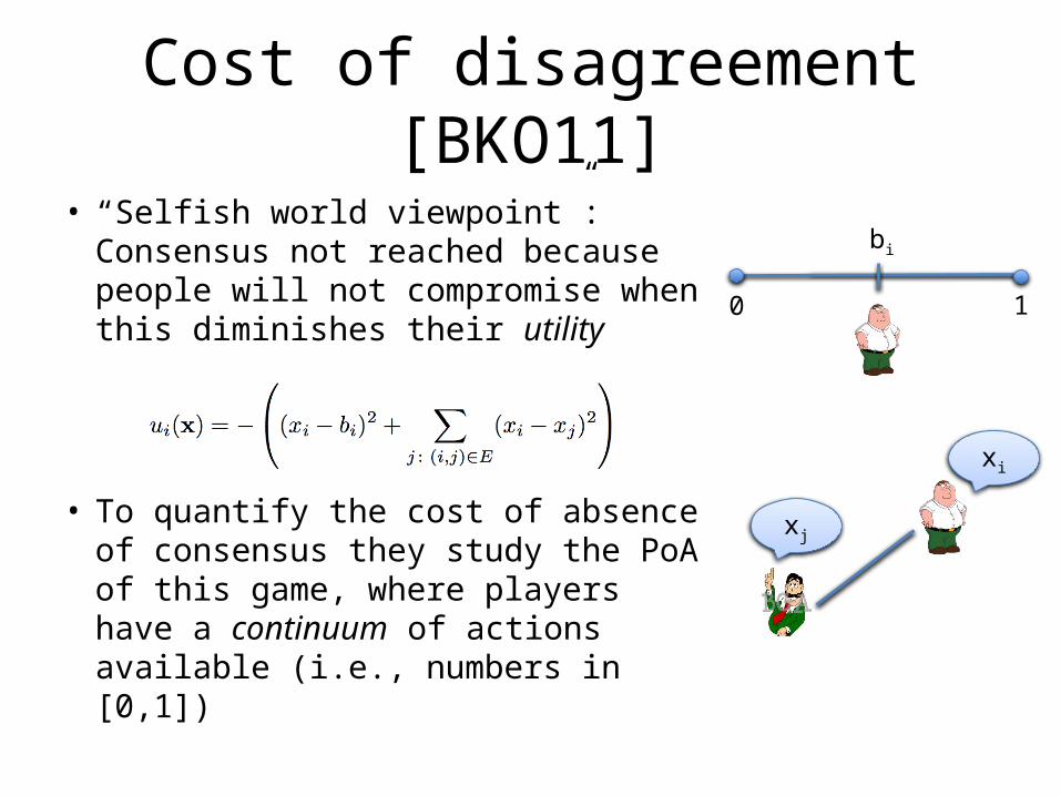
Cost of disagreement [BKO11]
• “Selfish world viewpoint”: Consensus not reached because people will not compromise when this diminishes their utility
• To quantify the cost of absence of consensus they study the PoA of this game, where players have a continuum of actions available (i.e., numbers in [0,1])
0 1
bi
xj
xi

OUR CONTRIBUTION
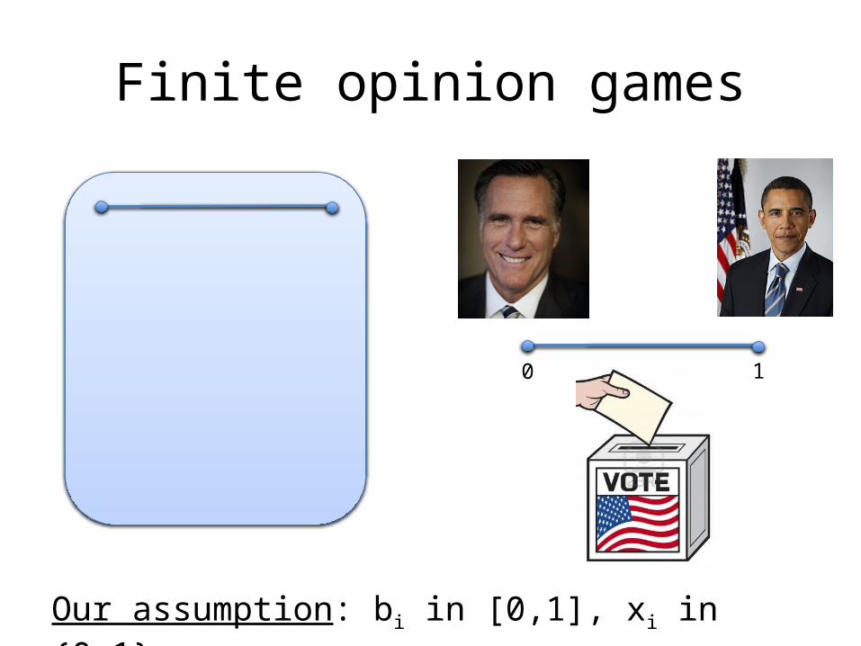
Finite opinion games
0 1
0 1
Our assumption: bi in [0,1], xi in {0,1}

Convergence rate of best-response dynamics
• Potential game with a polynomial potential function
• Convergence of best-response dynamics to pure Nash equilibria is polynomial: at each step the potential decreases by a constant
0 1.5.25 .75
xj
xi
xi ≠ xj

Noisy best-responses
• Utilities hard to determine exactly in real life!– … or otherwise, elections would be less uncertain
• Introducing noise
no noise: selection of strategy which maximizes the utility
player’s strategy set
noise: probability distribution over strategies
player’s strategy set

Logit dynamics [Blume, GEB93], [Auletta, Ferraioli, Pasquale, (Penna) & Persiano , 2010-ongoing]
• At each time step, from profile x1. Select a player uniformly at random, call him i2. Update his strategy to si with probability
proportional to
• β is the “rationality level” (inverse of the noise)– β = 0: strategy selected u.a.r. (no rationality)– β ∞: best response selected (full rationality)– β > 0: strategies promising higher utility have higher
chance of being used
Convergence of logit dynamics
• Nash equilibria are not the right solution concept for Logit dynamics
• Logit dynamics defines an ergodic Markov chain– unique stationary distribution exists
• Better than (P)NE!
– this distribution is the fixed point of the dynamics (logit equilibrium)
• How fast do we converge to the logit equilibrium as a function of β?– The answer requires to bound the mixing time of the
Markov chain defined by logit dynamics
Results
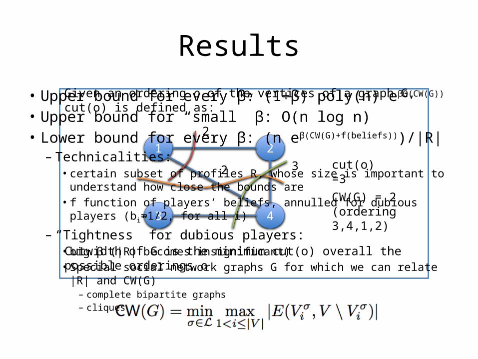
Given an ordering o of the vertices of a graph G, cut(o) is defined as:
Cutwidth of G is the minimum cut(o) overall the possible orderings o
1 2
3 4
2
2 3 cut(o)=3
CW(G) = 2 (ordering 3,4,1,2)
• Upper bound for every β: (1+β) poly(n) eβΘ(CW(G))
• Upper bound for “small” β: O(n log n) • Lower bound for every β: (n eβ(CW(G)+f(beliefs)))/|R|
– Technicalities: • certain subset of profiles R, whose size is important to understand how
close the bounds are• f function of players’ beliefs, annulled for dubious players (bi=1/2, for
all i)
– “Tightness” for dubious players:• big β (|R| becomes insignificant)• Special social network graphs G for which we can relate |R| and CW(G)
– complete bipartite graphs– cliques

Upper bound for “small” β: some details
• Hypothesis:– Social network graph G connected– More than 2 players– β ≤ 1/max degree of G
• Proof technique: – Coupling of probability distributions
• Result determines a border value for β, for which logit dynamics “looks like” a random walk on an hypercube
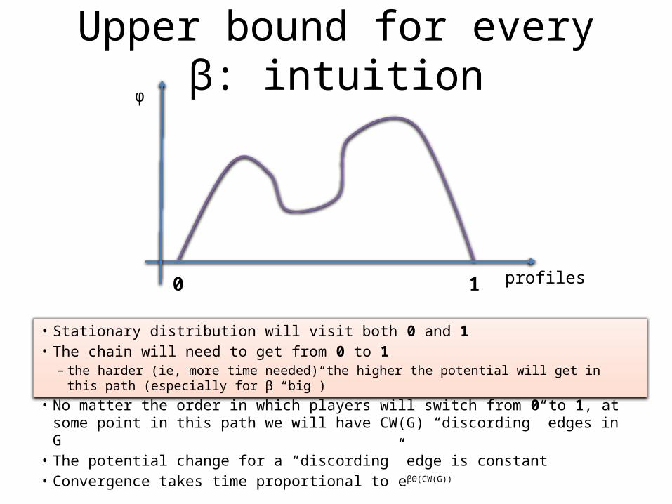
Upper bound for every β: intuition
• Stationary distribution will visit both 0 and 1 • The chain will need to get from 0 to 1
– the harder (ie, more time needed) the higher the potential will get in this path (especially for β “big”)
• No matter the order in which players will switch from 0 to 1, at some point in this path we will have CW(G) “discording” edges in G
• The potential change for a “discording” edge is constant• Convergence takes time proportional to eβΘ(CW(G))
profiles
φ
0 1
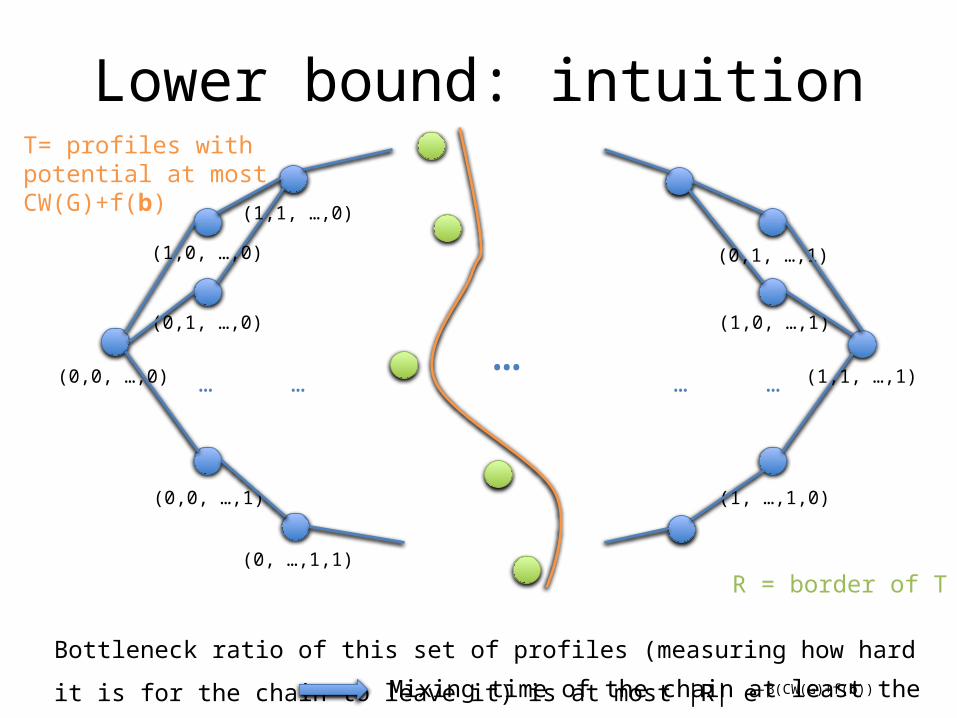
Lower bound: intuition
(0,1, …,0)
(0,0, …,1)
(0, …,1,1)
(1,0, …,1)
(1, …,1,0)
… ……
… …(0,0, …,0)
(1,1, …,0)
(0,1, …,1)
(1,1, …,1)
(1,0, …,0)
T= profiles with potential at most CW(G)+f(b)
Bottleneck ratio of this set of profiles (measuring how hard it is for the chain to leave it) is
at most |R| e-β(CW(G)+f(b))
R = border of T
Mixing time of the chain at least the inverse of the b.r.
Lower bound for specific social networks
• For complete bipartite graphs and cliques, we express the cutwidth as a function of number of players
• We bound the size of R• We can then relate |R| and CW(G) and obtain
a lower bound which shows that the factor eβCW(G) in the upper bound is necessary

Conclusions & open problems
• We consider a class of finite games motivated by sociology, psychology and economics
• We prove convergence rate bounds for best-response dynamics and logit dynamics
• Open questions:– Close the gap on the mixing time for all β/network
topologies– Consider weighted graphs?– More than two strategies?– Metastable distributions?
• [Auletta, Ferraioli, Pasquale & Persiano, SODA12]