Decentralized Collaborative Learning of Personalized

HAL Id: hal-01533182https://hal.inria.fr/hal-01533182

Submitted on 6 Jun 2017

HAL is a multi-disciplinary open accessarchive for the deposit and dissemination of sci-entific research documents, whether they are pub-lished or not. The documents may come fromteaching and research institutions in France orabroad, or from public or private research centers.

L’archive ouverte pluridisciplinaire HAL, estdestinée au dépôt et à la diffusion de documentsscientifiques de niveau recherche, publiés ou non,émanant des établissements d’enseignement et derecherche français ou étrangers, des laboratoirespublics ou privés.

Decentralized Collaborative Learning of PersonalizedModels over Networks

Paul Vanhaesebrouck, Aurélien Bellet, Marc Tommasi

To cite this version:Paul Vanhaesebrouck, Aurélien Bellet, Marc Tommasi. Decentralized Collaborative Learning of Per-sonalized Models over Networks. International Conference on Artificial Intelligence and Statistics(AISTATS), Apr 2017, Fort Lauderdale, Florida., United States. �hal-01533182�

https://hal.inria.fr/hal-01533182

https://hal.archives-ouvertes.fr

Decentralized Collaborative Learning ofPersonalized Models over Networks

Paul Vanhaesebrouck Aurelien Bellet Marc TommasiINRIA INRIA Universite de Lille

Abstract

We consider a set of learning agents in a col-laborative peer-to-peer network, where eachagent learns a personalized model accordingto its own learning objective. The questionaddressed in this paper is: how can agentsimprove upon their locally trained model bycommunicating with other agents that havesimilar objectives? We introduce and analyzetwo asynchronous gossip algorithms runningin a fully decentralized manner. Our first ap-proach, inspired from label propagation, aimsto smooth pre-trained local models over thenetwork while accounting for the confidencethat each agent has in its initial model. Inour second approach, agents jointly learn andpropagate their model by making iterativeupdates based on both their local dataset andthe behavior of their neighbors. To optimizethis challenging objective, our decentralizedalgorithm is based on ADMM.

1 Introduction

Increasing amounts of data are being produced by in-terconnected devices such as mobile phones, connectedobjects, sensors, etc. For instance, history logs aregenerated when a smartphone user browses the web,gives product ratings and executes various applica-tions. The currently dominant approach to extractuseful information from such data is to collect all users’personal data on a server (or a tightly coupled systemhosted in a data center) and apply centralized ma-chine learning and data mining techniques. However,this centralization poses a number of issues, such asthe need for users to “surrender” their personal data

Proceedings of the 20th International Conference on Artifi-cial Intelligence and Statistics (AISTATS) 2017, Fort Laud-erdale, Florida, USA. JMLR: W&CP volume 54. Copy-right 2017 by the author(s).

to the service provider without much control on howthe data will be used, while incurring potentially highbandwidth and device battery costs. Even when thelearning algorithm can be distributed in a way thatkeeps data on users’ devices, a central entity is of-ten still required for aggregation and coordination (seee.g., McMahan et al., 2016).

In this paper, we envision an alternative setting wheremany users (agents) with local datasets collaborateto learn models by engaging in a fully decentralizedpeer-to-peer network. Unlike existing work focusingon problems where agents seek to agree on a globalconsensus model (see e.g., Nedic and Ozdaglar, 2009;Wei and Ozdaglar, 2012; Duchi et al., 2012), we studythe case where each agent learns a personalized modelaccording to its own learning objective. We assumethat the network graph is given and reflects a notion ofsimilarity between agents (two agents are neighbors inthe network if they have a similar learning objective),but each agent is only aware of its direct neighbors.An agent can then learn a model from its (typicallyscarce) personal data but also from interactions withits neighborhood. As a motivating example, considera decentralized recommender system (Boutet et al.,2013, 2014) in which each user rates a small numberof movies on a smartphone application and expectspersonalized recommendations of new movies. In or-der to train a reliable recommender for each user, oneshould rely on the limited user’s data but also on in-formation brought by users with similar taste/profile.The peer-to-peer communication graph could be es-tablished when some users go the same movie theateror attend the same cultural event, and some similar-ity weights between users could be computed based onhistorical data (e.g., counting how many times peoplehave met in such locations).

Our contributions are as follows. After formalizing theproblem of interest, we propose two asynchronous andfully decentralized algorithms for collaborative learn-ing of personalized models. They belong to the fam-ily of gossip algorithms (Shah, 2009; Dimakis et al.,2010): agents only communicate with a single neigh-

Decentralized Collaborative Learning of Personalized Models over Networks

bor at a time, which makes our algorithms suitable fordeployment in large peer-to-peer real networks. Ourfirst approach, called model propagation, is inspired bythe graph-based label propagation technique of Zhouet al. (2004). In a first phase, each agent learns amodel based on its local data only, without communi-cating with others. In a second phase, the model pa-rameters are regularized so as to be smooth over thenetwork graph. We introduce some confidence valuesto account for potential discrepancies in the agents’training set sizes, and derive a novel asynchronous gos-sip algorithm which is simple and efficient. We provethat this algorithm converges to the optimal solutionof the problem. Our second approach, called collabo-rative learning, is more flexible as it interweaves learn-ing and propagation in a single process. Specifically,it optimizes a trade-off between the smoothness of themodel parameters over the network on the one hand,and the models’ accuracy on the local datasets on theother hand. For this formulation, we propose an asyn-chronous gossip algorithm based on a decentralizedversion of Alternating Direction Method of Multipliers(ADMM) (Boyd et al., 2011). Finally, we evaluate theperformance of our methods on two synthetic collabo-rative tasks: mean estimation and linear classification.Our experiments show the superiority of the proposedapproaches over baseline strategies, and confirm theefficiency of our decentralized algorithms.

The rest of the paper is organized as follows. Sec-tion 2 formally describes the problem of interest anddiscusses some related work. Our model propagationapproach is introduced in Section 3, along with our de-centralized algorithm. Section 4 describes our collab-orative learning approach, and derives an equivalentformulation which is amenable to optimization usingdecentralized ADMM. Finally, Section 5 shows our nu-merical results, and we conclude in Section 6.

2 Preliminaries

2.1 Notations and Problem Setting

We consider a set of n agents V = JnK where JnK :={1, . . . , n}. Given a convex loss function ` : Rp×X×Y,the goal of agent i is to learn a model θi ∈ Rp whose ex-pected loss E(xi,yi)∼µi

`(θi;xi, yi) is small with respectto an unknown and fixed distribution µi over X × Y.Each agent i has access to a set of mi ≥ 0 i.i.d. train-ing examples Si = {(xji , y

ji )}

mij=1 drawn from µi. We

allow the training set size to vary widely across agents(some may even have no data at all). This is impor-tant in practice as some agents may be more “active”than others, may have recently joined the service, etc.

In isolation, an agent i can learn a “solitary” model

θsoli by minimizing the loss over its local dataset Si:

θsoli ∈ arg minθ∈Rp

Li(θ) =

mi∑j=1

`(θ;xji , yji ). (1)

The goal for the agents is to improve upon their soli-tary model by leveraging information from other usersin the network. Formally, we consider a weighted con-nected graph G = (V,E) over the set V of agents,where E ⊆ V × V is the set of undirected edges.We denote by W ∈ Rn×n the symmetric nonneg-ative weight matrix associated with G, where Wij

gives the weight of edge (i, j) ∈ E and by conven-tion, Wij = 0 if (i, j) /∈ E or i = j. We assumethat the weights represent the underlying similaritybetween the agents’ objectives: Wij should tend to belarge (resp. small) when the objectives of agents i andj are similar (resp. dissimilar). While we assume inthis paper that the weights are given, in practical sce-narios one could for instance use some auxiliary infor-mation such as users’ profiles (when available) and/orprediction disagreement to estimate the weights. Fornotational convenience, we define the diagonal matrixD ∈ Rn×n where Dii =

∑nj=1Wij . We will also de-

note by Ni = {j 6= i : Wij > 0} the set of neighbors ofagent i. We assume that the agents only have a localview of the network: they know their neighbors andthe associated weights, but not the global topology orhow many agents participate in the network.

Our goal is to propose decentralized algorithms foragents to collaboratively improve upon their solitarymodel by leveraging information from their neighbors.

2.2 Related Work

Several peer-to-peer algorithms have been developedfor decentralized averaging (Kempe et al., 2003; Boydet al., 2006; Colin et al., 2015) and optimization (Nedicand Ozdaglar, 2009; Ram et al., 2010; Duchi et al.,2012; Wei and Ozdaglar, 2012, 2013; Iutzeler et al.,2013; Colin et al., 2016). These approaches solve aconsensus problem of the form:

minθ∈Rp

n∑i=1

Li(θ), (2)

resulting in a global solution common to all agents(e.g., a classifier minimizing the prediction error overthe union of all datasets). This is unsuitable for oursetting, where all agents have personalized objectives.

Our problem is reminiscent of Multi-Task Learning(MTL) (Caruana, 1997), where one jointly learns mod-els for related tasks. Yet, there are several differenceswith our setting. In MTL, the number of tasks is oftensmall, training sets are well-balanced across tasks, and

Paul Vanhaesebrouck, Aurelien Bellet, Marc Tommasi

all tasks are usually assumed to be positively related(a popular assumption is that all models share a com-mon subspace). Lastly, the algorithms are centralized,aside from the distributed MTL of Wang et al. (2016)which is synchronous and relies on a central server.

3 Model Propagation

In this section, we present our model propagation ap-proach. We first introduce a global optimization prob-lem, and then propose and analyze an asynchronousgossip algorithm to solve it.

3.1 Problem Formulation

In this formulation, we assume that each agent i haslearned a solitary model θsoli by minimizing its localloss, as in (1). This can be done without any com-munication between agents. Our goal here consists inadapting these models by making them smoother overthe network graph. In order account for the fact thatthe solitary models were learned on training sets ofdifferent sizes, we will use ci ∈ (0, 1] to denote the con-fidence we put in the model θsoli of user i ∈ {1, . . . , n}.The ci’s should be proportional to the number of train-ing points mi — one may for instance set ci = mi

maxj mj

(plus some small constant in the case where mi = 0).

Denoting Θ = [θ1; . . . ; θn] ∈ Rn×p, the objective func-tion we aim to minimize is as follows:

QMP (Θ) =1

2

( n∑i<j

Wij‖θi − θj‖2+

µ

n∑i=1

Diici‖θi − θsoli ‖2), (3)

where µ > 0 is a trade-off parameter and ‖·‖ denotesthe Euclidean norm. The first term in the right handside of (3) is a classic quadratic form used to smooththe models within neighborhoods: the distance be-tween the new models of agents i and j is encouragedto be small when the weight Wij is large. The sec-ond term prevents models with large confidence fromdiverging too much from their original values so thatthey can propagate useful information to their neigh-borhood. On the other hand, models with low confi-dence are allowed large deviations: in the extreme casewhere agent i has very little or even no data (i.e., ci isnegligible), its model is fully determined by the neigh-boring models. The presence of Dii in the second termis simply for normalization. We have the following re-sult (the proof is in the supplementary material).

Proposition 1 (Closed-form solution). Let P =D−1W be the stochastic similarity matrix associated

with the graph G and Θsol = [θsol1 ; . . . ; θsoln ] ∈ Rn×p.The solution Θ? = arg minΘ∈Rn×p QMP (Θ) is given by

Θ? = α(I − α(I − C)− αP )−1CΘsol , (4)

with α ∈ (0, 1) such that µ = (1−α)/α, and α = 1−α.

Our formulation is a generalization of the semi-supervised label propagation technique of (Zhou et al.,2004), which can be recovered by setting C = I (sameconfidence for all nodes). Note that it is strictly moregeneral: we can see from (4) that unless the confi-dence values are equal for all agents, the confidenceinformation cannot be incorporated by using differentsolitary models Θsol or by considering a different graph(because α

α (I − C) − P is not stochastic). The asyn-chronous gossip algorithm we present below thus ap-plies to label propagation for which, to the best of ourknowledge, no such algorithm was previously known.

Computing the closed form solution (4) requires theknowledge of the global network and of all solitarymodels, which are unknown to the agents. Our start-ing point for the derivation of an asynchronous gossipalgorithm is the following iterative form: for any t ≥ 0,

Θ(t+ 1) = (αI + αC)−1 (

αPΘ(t) + αCΘsol), (5)

The sequence (Θ(t))t∈N can be shown to converge to(4) regardless of the choice of initial value Θ(0), seesupplementary material for details. An interesting ob-servation about this recursion is that it can be decom-posed into agent-centric updates which only involveneighborhoods. Indeed, for any agent i and any t ≥ 0:

θi(t+ 1) =1

α+ αci

(α∑j∈Ni

Wij

Diiθj(t) + αciθ

soli

).

The iteration (5) can thus be understood as a decen-tralized but synchronous process where, at each step,every agent communicates with all its neighbors tocollect their current model parameters and uses thisinformation to update its model. Assuming that theagents do have access to a global clock to synchronizethe updates (which is unrealistic in many practical sce-narios), synchronization incurs large delays since allagents must finish the update at step t before anyonestarts step t + 1. The fact that agents must contactall their neighbors at each iteration further hinders theefficiency of the algorithm. To avoid these limitations,we propose below an asynchronous gossip algorithm.

3.2 Asynchronous Gossip Algorithm

In the asynchronous setting, each agent has a localclock ticking at the times of a rate 1 Poisson process,and wakes up when it ticks. As local clocks are i.i.d.,


it is equivalent to activating a single node uniformlyat random at each time step (Boyd et al., 2006).1

The idea behind our algorithm is the following. Atany time t ≥ 0, each agent i will maintain a (possi-bly outdated) knowledge of its neighbors’ models. Formathematical convenience, we will consider a matrixΘi(t) ∈ Rn×p where its i-th line Θi

i(t) ∈ Rp is agent i’s

model at time t, and for j 6= i, its j-th line Θji (t) ∈ Rp

is agent i’s last knowledge of the model of agent j. Forany j /∈ Ni ∪ {i} and any t ≥ 0, we will maintain

Θji (t) = 0. Let Θ = [Θ>1 , . . . , Θ

>n ]> ∈ Rn2×p be the

horizontal stacking of all the Θi’s.

If agent i wakes up at time step t, two consecutiveactions are performed:

• communication step: agent i selects a randomneighbor j ∈ Ni with prob. πji and both agentsupdate their knowledge of each other’s model:

Θji (t+ 1) = Θj

j(t) and Θij(t+ 1) = Θi

i(t),

• update step: agents i and j update their own mod-els based on current knowledge. For l ∈ {i, j}:

Θll(t+ 1) = (α+ αcl)

−1(α∑k∈Nl

Wlk

DllΘkl (t+ 1) + αclθ

soll

). (6)

All other variables in the network remain unchanged.In the communication step above, πji corresponds tothe probability that agent i selects agent j. For anyi ∈ JnK, we have πi ∈ [0, 1]

nsuch that

∑nj=1 π

ji = 1

and πji > 0 if and only if j ∈ Ni.

Our algorithm belongs to the family of gossip algo-rithms as each agent communicates with at most oneneighbor at a time. Gossip algorithms are known to bevery effective for decentralized computation in peer-to-peer networks (see Dimakis et al., 2010; Shah, 2009).Thanks to its asynchronous updates, our algorithm hasthe potential to be much faster than a synchronous ver-sion when executed in a large peer-to-peer network.

The main result of this section shows that our algo-rithm converges to a state where all nodes have theiroptimal model (and those of their neighbors).

Theorem 1 (Convergence). Let Θ(0) ∈ Rn2×p be

some arbitrary initial value and (Θ(t))t∈N be thesequence generated by our algorithm. Let Θ? =arg minΘ∈Rn×p QMP (Θ) be the optimal solution tomodel propagation. For any i ∈ JnK, we have:

limt→∞

E[Θji (t)]

= Θ?j for j ∈ Ni ∪ {i}.

1Our analysis straightforwardly extends to the casewhere agents have clocks ticking at different rates.

Sketch of proof. The first step of the proof is to rewritethe algorithm as an equivalent random iterative pro-cess over Θ ∈ Rn2×p of the form:

Θ(t+ 1) = A(t)Θ(t) + b(t),

for any t ≥ 0. Then, we show that the spectral radiusof E[A(t)] is smaller than 1, which allows us to exhibitthe convergence to the desired quantity. The proof canbe found in the supplementary material.

4 Collaborative Learning

In the approach presented in the previous section,models are learned locally by each agent and thenpropagated through the graph. In this section, weallow the agents to simultaneously learn their modeland propagate it through the network. In other words,agents iteratively update their models based on boththeir local dataset and the behavior of their neighbors.While in general this is computationally more costlythan merely propagating pre-trained models, we canexpect significant improvements in terms of accuracy.

As in the case of model propagation, we first intro-duce the global objective function and then proposean asynchronous gossip algorithm, which is based onthe general paradigm of ADMM (Boyd et al., 2011).

4.1 Problem Formulation

In contrast to model propagation, the objective func-tion to minimize here takes into account the loss ofeach personal model on the local dataset, rather thansimply the distance to the solitary model:

QCL(Θ) =

n∑i<j

Wij‖θi − θj‖2 + µ

n∑i=1

DiiLi(θi), (7)

where µ > 0 is a trade-off parameter. The associatedoptimization problem is Θ? = arg minΘ∈Rn×p QCL(Θ).

The first term in the right hand side of (7) is the sameas in the model propagation objective (3) and tends tofavor models that are smooth on the graph. However,while in model propagation enforcing smoothness onthe models may potentially translate into a significantdecrease of accuracy on the local datasets (even for rel-atively small changes in parameter values with respectto the solitary models), here the second term preventsthis. It allows more flexibility in settings where verydifferent parameter values define models which actu-ally give very similar predictions. Note that the con-fidence is built in the second term as Li is a sum overthe local dataset of agent i.

In general, there is no closed-form expression for Θ?,but we can solve the problem with a decentralized it-erative algorithm, as shown in the rest of this section.


4.2 Asynchronous Gossip Algorithm

We propose an asynchronous decentralized algorithmfor minimizing (7) based on the Alternative DirectionMethod of Multipliers (ADMM). This general methodis a popular way to solve consensus problems of theform (2) in the distributed and decentralized settings(see e.g., Boyd et al., 2011; Wei and Ozdaglar, 2012,2013; Iutzeler et al., 2013). In our setting, we do notseek a consensus in the classic sense of (2) since ourgoal is to learn a personalized model for each agent.However, we show below that we can reformulate (7)as an equivalent partial consensus problem which isamenable to decentralized optimization with ADMM.

Problem reformulation. Let Θi be the set of |Ni|+1variables θj ∈ Rp for j ∈ Ni∪{i}, and denote θj by Θj

i .This is similar to the notations used in Section 3, ex-cept that here we consider Θi as living in R(|Ni|+1)×p.We now define

QiCL(Θi) =1

2

∑j∈Ni

Wij‖θi − θj‖2 + µDiiLi(θi),

so that we can rewrite our problem (7) asminΘ∈Rn×p

∑ni=1QiCL(Θi).

In this formulation, the objective functions associatedwith the agents are dependent as they share some de-cision variables in Θ. In order to apply decentralizedADMM, we need to decouple the objectives. The ideais to introduce a local copy Θi ∈ R(|Ni|+1)×p of thedecision variables Θi for each agent i and to imposeequality constraints on the variables Θi

i = Θij for all

i ∈ JnK, j ∈ Ni. This partial consensus can be seen asrequiring that two neighboring agents agree on eachother’s personalized model. We further introduce 4secondary variables Ziei, Z

iej , Z

jei and Zjej for each edge

e = (i, j), which can be viewed as estimates of the

models Θi and Θj known by each end of e and will al-low an efficient decomposition of the ADMM updates.

Formally, denoting Θ = [Θ>1 , . . . , Θ>n ]> ∈ R(2|E|+n)×p

and Z ∈ R4|E|×p, we introduce the formulation

minΘ∈R(2|E|+n)×p

Z∈CE

n∑i=1

QiCL(Θi)

s.t. ∀e = (i, j) ∈ E,

{Ziei = Θi

i, Zjei = Θj

i

Zjej = Θjj , Z

iej = Θi

j ,

(8)

where CE = {Z ∈ R4|E|×p | Ziei = Ziej , Zjej = Zjei for

all e = (i, j) ∈ E}. It is easy to see that Problem (8) isequivalent to the original problem (7) in the following

sense: the minimizer Θ? of (8) satisfies (Θ?)ji = Θ?j

for all i ∈ JnK and j ∈ Ni ∪ {i}. Further observe

that the set of constraints involving Θ can be written

DΘ+HZ = 0 where H = −I of dimension 4|E|×4|E|is diagonal invertible and D of dimension 4|E|×(2|E|+n) contains exactly one entry of 1 in each row. Theassumptions of Wei and Ozdaglar (2013) are thus metand we can apply asynchronous decentralized ADMM.

Before presenting the algorithm, we derive the aug-mented Lagrangian associated with Problem (8). LetΛjei be dual variables associated with constraints

involving Θ in (8). For convenience, we denoteby Zi ∈ R2|Ni| the set of secondary variables{{Ziei} ∪ {Z

jei}}e=(i,j)∈E associated with agent i. Sim-

ilarly, we denote by Λi ∈ R2|Ni| the set of dual vari-ables {{Λiei} ∪ {Λ

jei}}e=(i,j)∈E . The augmented La-

grangian is given by:

Lρ(Θ, Z,Λ) =

n∑i=1

Liρ(Θi, Zi,Λi),

where ρ > 0 is a penalty parameter, Z ∈ CE and

Liρ(Θi, Zi,Λi) = QiCL(Θi)+∑

j:e=(i,j)∈E

[Λiei(Θ

ii−Ziei)

+Λjei(Θji −Z

jei)+

ρ

2

(‖Θi

i − Ziei‖2

+ ‖Θji − Z

jei‖

2) ].

Algorithm. ADMM consists in approximately min-imizing the augmented Lagrangian Lρ(Θ, Z,Λ) by al-ternating minimization with respect to the primal vari-able Θ and the secondary variable Z, together with aniterative update of the dual variable Λ.

We first briefly discuss how to instantiate the initialvalues Θ(0), Z(0) and Λ(0). The only constraint onthese initial values is to have Z(0) ∈ CE , so a simpleoption is to initialize all variables to 0. That said, itis typically advantageous to use a warm-start strategy.For instance, each agent i can send its solitary modelθsoli to its neighbors, and then set Θi

i = θsoli , Θji = θsolj

for all j ∈ Ni, Ziei = Θii, Z

jei = Θj

i for all e = (i, j) ∈ E,and Λ(0) = 0. Alternatively, one can initialize the al-gorithm with the model propagation solution obtainedusing the method of Section 3.

Recall from Section 3.2 that in the asynchronous set-ting, a single agent wakes up at each time step and se-lects one of its neighbors. Assume that agent i wakesup at some iteration t ≥ 0 and selects j ∈ Ni. Denot-ing e = (i, j), the iteration goes as follows:

1. Agent i updates its primal variables:

Θi(t+ 1) = arg minΘ∈R(|Ni|+1)×p

Liρ(Θ, Zi(t),Λi(t)),

and sends Θii(t + 1), Θj

i (t + 1),Λiei(t),Λjei(t) to

agent j. Agent j executes the same steps w.r.t. i.


2. Using Θjj(t + 1), Θi

j(t + 1),Λjej(t),Λiej(t) received

from j, agent i updates its secondary variables:

Ziei(t+ 1) =1

2

[1

ρ

(Λiei(t) + Λiej(t)

)+

Θii(t+ 1) + Θi

j(t+ 1)],

Zjei(t+ 1) =1

2

[1

ρ

(Λjej(t) + Λjei(t)

)+

Θjj(t+ 1) + Θj

i (t+ 1)].

Agent j updates its secondary variables symmet-rically, so by construction we have Z(t+ 1) ∈ CE .

3. Agent i updates its dual variables:

Λiei(t+ 1) = Λiei(t) + ρ(Θii(t+ 1)− Ziei(t+ 1)

),

Λjei(t+ 1) = Λjei(t) + ρ(Θji (t+ 1)− Zjei(t+ 1)

).

Agent j updates its dual variables symmetrically.

All other variables in the network remain unchanged.

Step 1 has a simple solution for some loss functionscommonly used in machine learning (such as quadraticand L1 loss), and when it is not the case ADMMis typically robust to approximate solutions to thecorresponding subproblems (obtained for instance af-ter a few steps of gradient descent), see Boyd et al.(2011) for examples and further practical considera-tions. Asynchronous ADMM converges almost surelyto an optimal solution at a rate of O(1/t) for convexobjective functions (see Wei and Ozdaglar, 2013).

5 Experiments

In this section, we provide numerical experiments toevaluate the performance of our decentralized algo-rithms with respect to accuracy, convergence rate andthe amount of communication. To this end, we intro-duce two synthetic collaborative tasks: mean estima-tion and linear classification.

5.1 Collaborative Mean Estimation

We first introduce a simple task in which the goalof each agent is to estimate the mean of a 1D dis-tribution. To this end, we adapt the two intertwin-ing moons dataset popular in semi-supervised learning(Zhou et al., 2004). We consider a set of 300 agents,together with auxiliary information about each agenti in the form of a vector vi ∈ R2. The true distribu-tion µi of an agent i is either N (1, 40) or N (−1, 40)depending on whether vi belongs to the upper or lowermoon, see Figure 1(a). Each agent i receives mi sam-ples x1

i , . . . , xmii ∈ R from its distribution µi. Its soli-

tary model is then given by θsoli = 1mi

∑mi

j=1 xji , which

corresponds to the use of the quadratic loss function`(θ;xi) = ‖θ − xi‖2. Finally, the graph over agents isthe complete graph where the weight between agents iand j is given by a Gaussian kernel on the agents’ aux-iliary information Wij = exp(−‖vi − vj‖2/2σ2), withσ = 0.1 for appropriate scaling. In all experiments,the parameter α of model propagation was set to 0.99,which gave the best results on a held-out set of randomproblem instances. We first use this mean estimationtask to illustrate the importance of considering con-fidence values in our model propagation formulation,and then to evaluate the efficiency of our asynchronousdecentralized algorithm.

Relevance of confidence values. Our goal here isto show that introducing confidence values into themodel propagation approach can significantly improvethe overall accuracy, especially when the agents re-ceive unbalanced amounts of data. In this experiment,we only compare model propagation with and withoutconfidence values, so we compute the optimal solutionsdirectly using the closed-form solution (4).

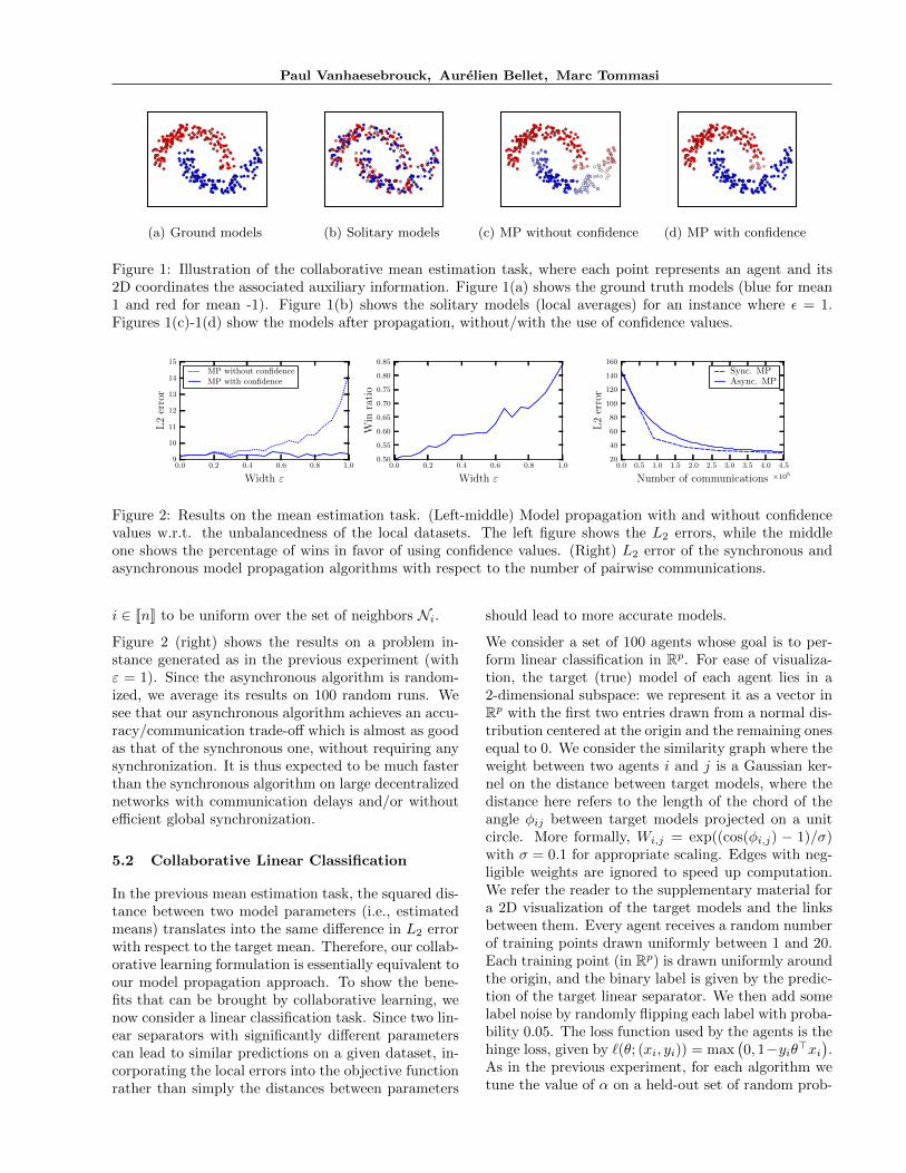
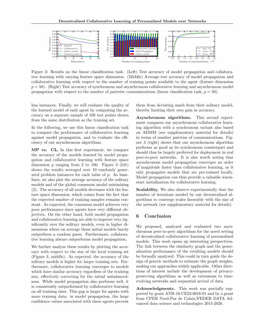
We generate several problem instances with varyingstandard deviation for the confidence values ci’s. Moreprecisely, we sample ci for each agent i from a uniformdistribution centered at 1/2 with width ε ∈ [0, 1]. Thenumber of samples mi given to agent i is then set tomi = dci · 100e. The larger ε, the more variance inthe size of the local datasets. Figures 1(b)-1(d) givea visualization of the models before and after propa-gation on a problem instance for the hardest settingε = 1. Figure 2 (left-middle) shows results averagedover 1000 random problem instances for several valuesof ε. As expected, when the local dataset sizes arewell-balanced (small ε), model propagation performsthe same with or without the use of confidence values.Indeed, both have similar L2 error with respect to thetarget mean, and the win ratio is about 0.5. However,the performance gap in favor of using confidence val-ues increases sharply with ε. For ε = 1, the win ratioin favor of using confidence values is about 0.85. Strik-ingly, the error of model propagation with confidencevalues remains constant as ε increases. These resultsempirically confirm the relevance of introducing confi-dence values into the objective function.

Asynchronous algorithm. In this second experi-ment, we compare asynchronous model propagationwith the synchronous variant given by (5). We areinterested in the average L2 error of the models as afunction of the number of pairwise communications(number of exchanges from one agent to another).Note that a single iteration of the synchronous (resp.asynchronous) algorithm corresponds to 2|E| (resp.2) communications. For the asynchronous algorithm,we set the neighbor selection distribution πi of agent


(a) Ground models (b) Solitary models (c) MP without confidence (d) MP with confidence

Figure 1: Illustration of the collaborative mean estimation task, where each point represents an agent and its2D coordinates the associated auxiliary information. Figure 1(a) shows the ground truth models (blue for mean1 and red for mean -1). Figure 1(b) shows the solitary models (local averages) for an instance where ε = 1.Figures 1(c)-1(d) show the models after propagation, without/with the use of confidence values.

0.0 0.2 0.4 0.6 0.8 1.0

Width ε

9

10

11

12

13

14

15

L2error

MP without confidenceMP with confidence

0.0 0.2 0.4 0.6 0.8 1.0

Width ε

0.50

0.55

0.60

0.65

0.70

0.75

0.80

0.85W

inratio

0.0 0.5 1.0 1.5 2.0 2.5 3.0 3.5 4.0 4.5

Number of communications ×105

20

40

60

80

100

120

140

160

L2error

Sync. MPAsync. MP

Figure 2: Results on the mean estimation task. (Left-middle) Model propagation with and without confidencevalues w.r.t. the unbalancedness of the local datasets. The left figure shows the L2 errors, while the middleone shows the percentage of wins in favor of using confidence values. (Right) L2 error of the synchronous andasynchronous model propagation algorithms with respect to the number of pairwise communications.

i ∈ JnK to be uniform over the set of neighbors Ni.

Figure 2 (right) shows the results on a problem in-stance generated as in the previous experiment (withε = 1). Since the asynchronous algorithm is random-ized, we average its results on 100 random runs. Wesee that our asynchronous algorithm achieves an accu-racy/communication trade-off which is almost as goodas that of the synchronous one, without requiring anysynchronization. It is thus expected to be much fasterthan the synchronous algorithm on large decentralizednetworks with communication delays and/or withoutefficient global synchronization.

5.2 Collaborative Linear Classification

In the previous mean estimation task, the squared dis-tance between two model parameters (i.e., estimatedmeans) translates into the same difference in L2 errorwith respect to the target mean. Therefore, our collab-orative learning formulation is essentially equivalent toour model propagation approach. To show the bene-fits that can be brought by collaborative learning, wenow consider a linear classification task. Since two lin-ear separators with significantly different parameterscan lead to similar predictions on a given dataset, in-corporating the local errors into the objective functionrather than simply the distances between parameters

should lead to more accurate models.

We consider a set of 100 agents whose goal is to per-form linear classification in Rp. For ease of visualiza-tion, the target (true) model of each agent lies in a2-dimensional subspace: we represent it as a vector inRp with the first two entries drawn from a normal dis-tribution centered at the origin and the remaining onesequal to 0. We consider the similarity graph where theweight between two agents i and j is a Gaussian ker-nel on the distance between target models, where thedistance here refers to the length of the chord of theangle φij between target models projected on a unitcircle. More formally, Wi,j = exp((cos(φi,j) − 1)/σ)with σ = 0.1 for appropriate scaling. Edges with neg-ligible weights are ignored to speed up computation.We refer the reader to the supplementary material fora 2D visualization of the target models and the linksbetween them. Every agent receives a random numberof training points drawn uniformly between 1 and 20.Each training point (in Rp) is drawn uniformly aroundthe origin, and the binary label is given by the predic-tion of the target linear separator. We then add somelabel noise by randomly flipping each label with proba-bility 0.05. The loss function used by the agents is thehinge loss, given by `(θ; (xi, yi)) = max

(0, 1−yiθ>xi

).

As in the previous experiment, for each algorithm wetune the value of α on a held-out set of random prob-


0 20 40 60 80 100

Dimension p

0.50

0.55

0.60

0.65

0.70

0.75

0.80

0.85

0.90

0.95

Tes

tacc

ura

cy

Model P.

Collaborative L.

Solitary models

Consensus model

5 10 15 20

Number of training points

0.0

0.1

0.2

0.3

0.4

0.5

0.6

0.7

0.8

0.9

Tes

tacc

ura

cy

Collaborative Learning

Model Propagation

Solitary models

0.0 0.5 1.0 1.5 2.0 2.5 3.0 3.5

Number of communications ×105

0.60

0.65

0.70

0.75

0.80

0.85

Tes

tacc

ura

cy

Sync. CL

Async. CL

Async. MP

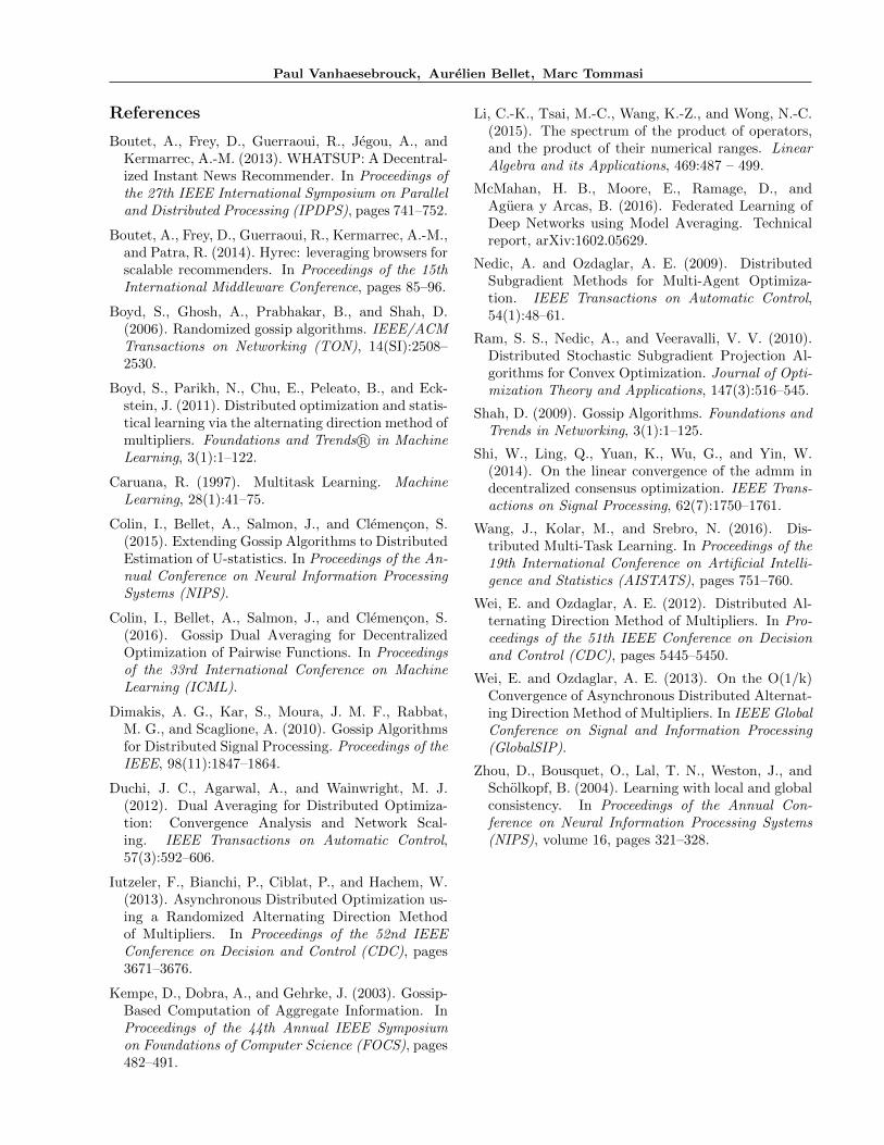
Figure 3: Results on the linear classification task. (Left) Test accuracy of model propagation and collabora-tive learning with varying feature space dimension. (Middle) Average test accuracy of model propagation andcollaborative learning with respect to the number of training points available to the agent (feature dimensionp = 50). (Right) Test accuracy of synchronous and asynchronous collaborative learning and asynchronous modelpropagation with respect to the number of pairwise communications (linear classification task, p = 50).

lem instances. Finally, we will evaluate the quality ofthe learned model of each agent by computing the ac-curacy on a separate sample of 100 test points drawnfrom the same distribution as the training set.

In the following, we use this linear classification taskto compare the performance of collaborative learningagainst model propagation, and to evaluate the effi-ciency of our asynchronous algorithms.

MP vs. CL. In this first experiment, we comparethe accuracy of the models learned by model propa-gation and collaborative learning with feature spacedimension p ranging from 2 to 100. Figure 3 (left)shows the results averaged over 10 randomly gener-ated problem instances for each value of p. As base-lines, we also plot the average accuracy of the solitarymodels and of the global consensus model minimizing(2). The accuracy of all models decreases with the fea-ture space dimension, which comes from the fact thatthe expected number of training samples remains con-stant. As expected, the consensus model achieves verypoor performance since agents have very different ob-jectives. On the other hand, both model propagationand collaborative learning are able to improve very sig-nificantly over the solitary models, even in higher di-mensions where on average these initial models barelyoutperform a random guess. Furthermore, collabora-tive learning always outperforms model propagation.

We further analyze these results by plotting the accu-racy with respect to the size of the local training set(Figure 3, middle). As expected, the accuracy of thesolitary models is higher for larger training sets. Fur-thermore, collaborative learning converges to modelswhich have similar accuracy regardless of the trainingsize, effectively correcting for the initial unbalanced-ness. While model propagation also performs well, itis consistently outperformed by collaborative learningon all training sizes. This gap is larger for agents withmore training data: in model propagation, the largeconfidence values associated with these agents prevent

them from deviating much from their solitary model,thereby limiting their own gain in accuracy.

Asynchronous algorithms. This second experi-ment compares our asynchronous collaborative learn-ing algorithm with a synchronous variant also basedon ADMM (see supplementary material for details)in terms of number pairwise of communications. Fig-ure 3 (right) shows that our asynchronous algorithmperforms as good as its synchronous counterpart andshould thus be largely preferred for deployment in realpeer-to-peer networks. It is also worth noting thatasynchronous model propagation converges an orderof magnitude faster than collaborative learning, as itonly propagates models that are pre-trained locally.Model propagation can thus provide a valuable warm-start initialization for collaborative learning.

Scalability. We also observe experimentally that thenumber of iterations needed by our decentralized al-gorithms to converge scales favorably with the size ofthe network (see supplementary material for details).

6 Conclusion

We proposed, analyzed and evaluated two asyn-chronous peer-to-peer algorithms for the novel settingof decentralized collaborative learning of personalizedmodels. This work opens up interesting perspectives.The link between the similarity graph and the gener-alization performance of the resulting models shouldbe formally analyzed. This could in turn guide the de-sign of generic methods to estimate the graph weights,making our approaches widely applicable. Other direc-tions of interest include the development of privacy-preserving algorithms as well as extensions to time-evolving networks and sequential arrival of data.

Acknowledgments. This work was partially sup-ported by grant ANR-16-CE23-0016-01 and by a grantfrom CPER Nord-Pas de Calais/FEDER DATA Ad-vanced data science and technologies 2015-2020.


References

Boutet, A., Frey, D., Guerraoui, R., Jegou, A., andKermarrec, A.-M. (2013). WHATSUP: A Decentral-ized Instant News Recommender. In Proceedings ofthe 27th IEEE International Symposium on Paralleland Distributed Processing (IPDPS), pages 741–752.

Boutet, A., Frey, D., Guerraoui, R., Kermarrec, A.-M.,and Patra, R. (2014). Hyrec: leveraging browsers forscalable recommenders. In Proceedings of the 15thInternational Middleware Conference, pages 85–96.

Boyd, S., Ghosh, A., Prabhakar, B., and Shah, D.(2006). Randomized gossip algorithms. IEEE/ACMTransactions on Networking (TON), 14(SI):2508–2530.

Boyd, S., Parikh, N., Chu, E., Peleato, B., and Eck-stein, J. (2011). Distributed optimization and statis-tical learning via the alternating direction method ofmultipliers. Foundations and Trends R© in MachineLearning, 3(1):1–122.

Caruana, R. (1997). Multitask Learning. MachineLearning, 28(1):41–75.

Colin, I., Bellet, A., Salmon, J., and Clemencon, S.(2015). Extending Gossip Algorithms to DistributedEstimation of U-statistics. In Proceedings of the An-nual Conference on Neural Information ProcessingSystems (NIPS).

Colin, I., Bellet, A., Salmon, J., and Clemencon, S.(2016). Gossip Dual Averaging for DecentralizedOptimization of Pairwise Functions. In Proceedingsof the 33rd International Conference on MachineLearning (ICML).

Dimakis, A. G., Kar, S., Moura, J. M. F., Rabbat,M. G., and Scaglione, A. (2010). Gossip Algorithmsfor Distributed Signal Processing. Proceedings of theIEEE, 98(11):1847–1864.

Duchi, J. C., Agarwal, A., and Wainwright, M. J.(2012). Dual Averaging for Distributed Optimiza-tion: Convergence Analysis and Network Scal-ing. IEEE Transactions on Automatic Control,57(3):592–606.

Iutzeler, F., Bianchi, P., Ciblat, P., and Hachem, W.(2013). Asynchronous Distributed Optimization us-ing a Randomized Alternating Direction Methodof Multipliers. In Proceedings of the 52nd IEEEConference on Decision and Control (CDC), pages3671–3676.

Kempe, D., Dobra, A., and Gehrke, J. (2003). Gossip-Based Computation of Aggregate Information. InProceedings of the 44th Annual IEEE Symposiumon Foundations of Computer Science (FOCS), pages482–491.

Li, C.-K., Tsai, M.-C., Wang, K.-Z., and Wong, N.-C.(2015). The spectrum of the product of operators,and the product of their numerical ranges. LinearAlgebra and its Applications, 469:487 – 499.

McMahan, H. B., Moore, E., Ramage, D., andAguera y Arcas, B. (2016). Federated Learning ofDeep Networks using Model Averaging. Technicalreport, arXiv:1602.05629.

Nedic, A. and Ozdaglar, A. E. (2009). DistributedSubgradient Methods for Multi-Agent Optimiza-tion. IEEE Transactions on Automatic Control,54(1):48–61.

Ram, S. S., Nedic, A., and Veeravalli, V. V. (2010).Distributed Stochastic Subgradient Projection Al-gorithms for Convex Optimization. Journal of Opti-mization Theory and Applications, 147(3):516–545.

Shah, D. (2009). Gossip Algorithms. Foundations andTrends in Networking, 3(1):1–125.

Shi, W., Ling, Q., Yuan, K., Wu, G., and Yin, W.(2014). On the linear convergence of the admm indecentralized consensus optimization. IEEE Trans-actions on Signal Processing, 62(7):1750–1761.

Wang, J., Kolar, M., and Srebro, N. (2016). Dis-tributed Multi-Task Learning. In Proceedings of the19th International Conference on Artificial Intelli-gence and Statistics (AISTATS), pages 751–760.

Wei, E. and Ozdaglar, A. E. (2012). Distributed Al-ternating Direction Method of Multipliers. In Pro-ceedings of the 51th IEEE Conference on Decisionand Control (CDC), pages 5445–5450.

Wei, E. and Ozdaglar, A. E. (2013). On the O(1/k)Convergence of Asynchronous Distributed Alternat-ing Direction Method of Multipliers. In IEEE GlobalConference on Signal and Information Processing(GlobalSIP).

Zhou, D., Bousquet, O., Lal, T. N., Weston, J., andScholkopf, B. (2004). Learning with local and globalconsistency. In Proceedings of the Annual Con-ference on Neural Information Processing Systems(NIPS), volume 16, pages 321–328.


SUPPLEMENTARY MATERIAL

A Proof of Proposition 1

Proposition 1 (Closed-form solution). Let P = D−1W be the stochastic similarity matrix associated with thegraph G and Θsol = [θsol1 ; . . . ; θsoln ] ∈ Rn×p. The solution Θ? = arg minΘ∈Rn×p QMP (Θ) is given by

Θ? = α(I − α(I − C)− αP )−1CΘsol ,

with α ∈ (0, 1) such that µ = α/α, and α = 1− α.

Proof. We write the objective function in matrix form:

QMP (Θ) =1

2

(tr [Θ>LΘ] + µ tr [(Θ−Θsol)

>DC(Θ−Θsol)]

),

where L = D −W is the graph Laplacian matrix and tr denotes the trace of a matrix. As QMP (Θ) is convexand quadratic in Θ, we can find its global minimum by setting its derivative to 0.

∇QMP (Θ) = LΘ + µDC(Θ−Θsol)

= LΘ∗ + µDC(Θ∗ −Θsol)

= (D −W + µDC)Θ∗ − µDCΘsol .

Hence,

∇QMP (Θ) = 0⇔ (I − P + µC)Θ∗ − µCΘsol = 0

⇔ (I − α(I − C)− αP )Θ∗ − αCΘsol = 0,

with µ = α/α. Since P is a stochastic matrix, its eigenvalues are in [−1, 1]. Moreover, (I − C)ii < 1 for all i,thus ρ(α(I − C) + αP ) < 1 where ρ(·) denotes the spectral radius. Consequently, I− α(I−C)−αP is invertibleand we get the desired result.

B Convergence of the Iterative Form (5)

We can rewrite the equation

Θ(t+ 1) = (αI + αC)−1 (

αPΘ(t) + αCΘsol), (5)

as

Θ(t) =(

(αI + αC)−1αP)t

Θ(0) +

t−1∑k=0

((αI + αC)

−1αP)k

(αI + αC)−1αCΘsol .

Since α(α+αci)

< 1 for any i ∈ JnK, we have ρ(

(αI + αC)−1αP)< 1 and therefore:

limt→∞

((αI + αC)

−1αP)t

= 0,

hence

limt→∞

Θ(t) =(I − (αI + αC)

−1αP)−1

(αI + αC)−1αCΘsol

= (I − α(I − C)− αP )−1αCΘsol

= Θ∗.


C Proof of Theorem 1

Theorem 1 (Convergence). Let Θ(0) ∈ Rn2×p be some arbitrary initial value and (Θ(t))t∈N be the sequencegenerated by our model propagation algorithm. Let Θ? = arg minΘ∈Rn×p QMP (Θ) be the optimal solution to modelpropagation. For any i ∈ JnK, we have:

limt→∞

E[Θji (t)]

= Θ?j for j ∈ Ni ∪ {i}.

Proof. In order to prove the convergence of our algorithm, we need to introduce an equivalent formulation as arandom iterative process over Θ ∈ Rn2×p, the horizontal stacking of all the Θi’s.

The communication step of agent i with its neighbor j consists in overwriting Θji and Θi

j with respectively Θjj

and Θii. This step will be handled by multiplication with the matrix O(i, j) ∈ Rn2×n2

defined as

O(i, j) = I + eji (ejj − e

ji )> + eij(e

ii − eij)>,

where for i, j ∈ JnK, the vector eji ∈ Rn2

has 1 as its (i− 1)n+ j-th coordinate and 0 in all others.

The update step of node i and j consists in replacing Θii and Θj

j with respectively the i-th line of

(αI + αC)−1(

αP Θi + αCΘsol)

and the j-th line of (αI + αC)−1(

αP Θj + αCΘsol). This step will be han-

dled by multiplication with the matrix U(i, j) ∈ Rn2×n2

and addition of the vector u(i, j) ∈ Rn2×p defined asfollows:

U(i, j) = I + (eiiei>i + ejje

j>j )(M − I)

u(i, j) = (eiiei>i + ejje

j>j )(αI + αC)

−1αCΘsol ,

where M ∈ Rn2×n2

is a block diagonal matrix with repetitions of (αI + αC)−1αP on the diagonal and Θsol ∈

Rn2×p is built by stacking horizontally n times the matrix Θsol .

We can now write down a global iterative process which is equivalent to our model propagation algorithm. Forany t ≥ 0:

Θ(t+ 1) = A(t)Θ(t) + b(t)

where, {A(t) = IEU(i, j)O(i, j)

b(t) = u(i, j)w.p.

πjin

for i, j ∈ J1, nK,

and IE is a n2 × n2 diagonal matrix with its (i− 1)n+ j-th value equal to 1 if (i, j) ∈ E or i = j and equal to0 otherwise. Note that IE is used simply to simplify our analysis by setting to 0 the lines of A(t) correspondingto non-existing edges (which can be safely ignored).

First, let us write the expected value of Θ(t) given Θ(t− 1):

E[Θ(t)|Θ(t− 1)

]= E[A(t)]Θ(t− 1) + E[b(t)]. (9)

Since the A(t)’s and b(t)’s are i.i.d., for any t ≥ 0 we have A = E[A(t)] and b = E[b(t)] where

A =1

nIE

n∑i,j

πjiU(i, j)O(i, j),

b =1

n

n∑i,j

πji u(i, j).

In order to prove Theorem 1, we first need to show that ρ(A) < 1, where ρ(A) denotes the spectral radius of A.

First, recall that ρ(

(αI + αC)−1αP)< 1 (see Appendix B). We thus have ρ(M) < 1 by construction of M and

λ(I −M) ⊂ (0, 2),


where λ(·) denotes the spectrum of a matrix. Furthermore, from the properties in Li et al. (2015) we know that

λ(

(eiiei>i + ejje

j>j )(I −M)

)⊂ [0, 2],

and finally we have:

λ(I + (eiie

i>i + ejje

j>j )(M − I)

)= λ(U(i, j)) ⊂ [−1, 1].

As we also have λ(O(i, j)) ⊂ [0, 1] therefore

λ (U(i, j)O(i, j)) ⊂ [−1, 1].

Let us first suppose that −1 is an eigenvalue of U(i, j)O(i, j) associated with the eigenvector v. From theprevious inequalities we deduce that v must be an eigenvector of O(i, j) associated with the eigenvalue +1 andan eigenvector of U(i, j) associated with the eigenvalue −1. Then from v = O(i, j)v we have vji = vjj and vij = vii .

From −v = U(i, j)v we can deduce that vlk = 0 for any k 6= l or k = l ∈ JnK\{i, j}. Finally we can see that

vii = vjj = 0 and therefore v = 0. This proves by contradiction that −1 is not an eigenvalue of U(i, j)O(i, j) and

furthermore that −1 is not an eigenvalue of A.

Let us now suppose that +1 is an eigenvalue of A, associated with the eigenvector v ∈ Rn2

. This would implythat

v = Av =1

nIE

n∑i,j

πjiU(i, j)O(i, j)v.

This can be expressed line by line as the following set of equations:

n∑k=1

(πk1 + π1k)v1

1 = e1>1

n∑k=1

(πk1 + π1k)MO(1, k)v

(π21 + π1

2)v21 = (π2

1 + π12)v2

2 if (1, 2) ∈ E else v21 = 0

(π31 + π1

3)v31 = (π3

1 + π13)v3

3 if (1, 3) ∈ E else v31 = 0

...

(π12 + π2

1)v12 = (π1

2 + π21)v1

1 if (2, 1) ∈ E else v12 = 0

n∑k=1

(πk2 + π2k)v2

2 = e2>2

n∑k=1

(πk2 + π2k)MO(2, k)v

(π32 + π2

3)v32 = (π3

2 + π23)v3

3 if (2, 3) ∈ E else v32 = 0

...

(πn−2n + πnn−2)vn−2

n = (πn−2n + πnn−2)vn−2

n−2 if (n, n− 2) ∈ E else vn−2n = 0

(πn−1n + πnn−1)vn−1

n = (πn−1n + πnn−1)vn−1

n−1 if (n, n− 1) ∈ E else vn−1n = 0

n∑k=1

(πkn + πnk )vnn = en>n

n∑k=1

(πkn + πnk )MO(n, k)v

We can rewrite the above system as

vji =

{vj if (i, j) ∈ E or i = j

0 otherwise,

0 =(I − (αI + αC)

−1αP)v.

(10)

with v ∈ Rn×p. As seen in Appendix B, the matrix I − α(I − C)− αP is invertible. Consequently v = 0 andthus v = 0, which proves by contradiction that +1 is not an eigenvalue of A.


Now that we have shown that ρ(A) < 1, let us write the expected value of Θ(t) by “unrolling” the recursion (9):

E[Θ(t)

]= AtΘ(0) +

t−1∑k=0

Ak b.

Let us denote Θ∗ = limt→∞

E[Θ(t)

]. Because ρ(A) < 1, we can write

Θ∗ = (I − A)−1b,

and finally(I − A)Θ∗ = b.

Similarly as in (10), we can identify Θ ∈ Rn×p such that

Θj∗i =

{Θj if (i, j) ∈ E or i = j

0 otherwise,

αCΘsol = (I − α(I − C) + αP )Θ.

Recalling the results from Appendix A, we have

Θ = α(I − α(I − C)− αP )−1CΘsol ,

and we thus haveΘ = Θ∗ = arg min

Θ∈Rn×p

QMP (Θ),

and the theorem follows.

D Synchronous Decentralized ADMM Algorithm for Collaborative Learning

For completeness, we present here the synchronous decentralized ADMM algorithm for collaborative learning.Based on our reformulation of Section 4.2 and following Wei and Ozdaglar (2012), the algorithm to find Θ?

consists in iterating over the following steps, starting at t = 0:

1. Every agent i ∈ JnK updates its primal variables:

Θi(t+ 1) = arg minΘ∈R(|Ni|+1)×p

Liρ(Θ, Zi(t),Λi(t)),

and sends Θii(t+ 1), Θj

i (t+ 1),Λiei(t),Λjei(t) to agent j for all j ∈ Ni.

2. Using values received by its neighbors, every agent i ∈ JnK updates its secondary variables for all e = (i, j) ∈E such that j ∈ Ni:

Ziei(t+ 1) =1

2

[1

ρ

(Λiei(t) + Λiej(t)

)+ Θi

i(t+ 1) + Θij(t+ 1)

],

Zjei(t+ 1) =1

2

[1

ρ

(Λjej(t) + Λjei(t)

)+ Θj

j(t+ 1) + Θji (t+ 1)

].

By construction, this update maintains Z(t+ 1) ∈ CE .

3. Every agent i ∈ JnK updates its dual variables for all e = (i, j) ∈ E such that j ∈ Ni:

Λiei(t+ 1) = Λiei(t) + ρ(Θii(t+ 1)− Ziei(t+ 1)

),

Λjei(t+ 1) = Λjei(t) + ρ(Θji (t+ 1)− Zjei(t+ 1)

).

Synchronous ADMM is known to converge to an optimal solution at rate O(1/t) when the objective functionis convex (Wei and Ozdaglar, 2012), and at a faster (linear) rate when it is strongly convex (Shi et al., 2014).However, it requires global synchronization across the network, which can be very costly in practice.


−3 −2 −1 0 1 2 3−2.0

−1.5

−1.0

−0.5

0.0

0.5

1.0

1.5

2.0

Figure 4: Target models of the agents (represented as points in R2) for the collaborative linear classification task.Two models are linked together when the angle between them is small, which corresponds to a small Euclideandistance after projection onto the unit circle.

100 200 300 400 500 600 700 800 900 1000

Number of agents

0

1

2

3

4

5

6

7

8

Nu

mb

erof

com

mu

nic

ati

on

s ×104

Sync. CL

Async. CL

Async. MP

Figure 5: Number of pairwise communications needed to reach 90% of the accuracy of the optimal models withvarying number of agents (linear classification task, p = 50).

E Additional Experimental Results

Target models in collaborative linear classification For the experiment of Section 5.2, Figure 4 showsthe target models of the agents as well as the links between them. We can see that the target models canbe very different from an agent to another, and that two agents are linked when there is a small enough (yetnon-negligible) angle between their target models.

Scalability with respect to the number of nodes In this experiment, we study how the number of iterationsneeded by our decentralized algorithms to converge to good solutions scale with the size of the network. Wefocus on the collaborative linear classification task introduced in Section 5.2 with the number n of agents rangingfrom 100 to 1000. The network is a k-nearest neighbor graph: each agent is linked to the k agents for which theangle similarity introduced in Section 5.2 is largest, and Wij = 1 if i and j are neighbors and 0 otherwise.

Figure 5 shows the number of iterations needed by our algorithms to reach 90% of the accuracy of the optimal setof models. We can see that the number of iterations scales linearly with n. In asynchronous gossip algorithms,the number of iterations that can be done in parallel also scales roughly linearly with n, so we can expect ouralgorithms to scale nicely to very large networks.

Documents

Decentralized Collaborative Learning of Personalized