Embed Size (px)
Citation preview
Decentralized charging decisions for the smart grid Stella Viktoria Schieffer Supervisors: Prof. Dr. Kay Axhausen Rashid A. Waraich
MasterThesis Institute for Transport Planning and Systems Spring 2011

B
1. Table of Contents 1. Introduction ........................................................................................................................ 1
2. Conceptual design ............................................................................................................... 3
2.1 Qualitative requirements of the decentralized smart charger ............................................. 3
2.2 Charging decision and slot booking ....................................................................................... 4
It is the goal of the decentralized smart charger to find charging times for each agent which ... 4
2.2.1. Agent constraints ........................................................................................................ 4
2.2.2. Global optimum........................................................................................................... 5
2.2.3. Minimal information ................................................................................................... 5
2.3. V2G ............................................................................................................................................ 9
2.3.1. The stochastic load ...................................................................................................... 9
2.3.2. The V2G decision ....................................................................................................... 10
2.3.3. Optimal solution ........................................................................................................ 10
3. Implementation ................................................................................................................ 12
3.1 The simulation framework MATSim .................................................................................... 12
3.2 The decentralized smart charger ........................................................................................ 13
3.2.1. Inputs......................................................................................................................... 13
3.2.2. Outputs ...................................................................................................................... 14
3.2.2. Charging time optimization procedure ..................................................................... 15
3.3 The V2G procedure ............................................................................................................. 25
3.3.1. Inputs......................................................................................................................... 25
3.3.2. Outputs ...................................................................................................................... 26
3.3.3. Procedure .................................................................................................................. 26
3.4 Runtime performance ......................................................................................................... 31
4. Simulations ....................................................................................................................... 38
4.1. Assessing the influence of EVs, prices, battery sizes and contract types on the system ........ 38
4.1.1. Input parameters and Setup ..................................................................................... 38
4.2. Additional tests ........................................................................................................................ 44
4.2.1. V2G Saturation limit .................................................................................................. 44
4.2.2. Charging speed .......................................................................................................... 45
5. Simulation Results............................................................................................................. 46
5.1. Influence of factors ............................................................................................................. 46
5.1.1. EV Failures ................................................................................................................ 47
5.1.2. Charging duration .................................................................................................... 49
5.1.3. Charging cost ............................................................................................................ 51
5.1.4. PHEV Emissions ........................................................................................................ 55
C
5.1.5. V2G Regulation ........................................................................................................ 57
5.1.6. V2G Revenue ............................................................................................................ 64
5.1.7. Effectiveness in regulating the grid .......................................................................... 70
5.1.8. Effectiveness in V2G regulation ............................................................................... 73
5.2. Additional tests ................................................................................................................... 76
5.2.1. V2G saturation limit ................................................................................................. 76
5.2.2. Charging speed ......................................................................................................... 80
6. Discussion ......................................................................................................................... 90
6.1. Decentralized Smart Charging Algorithm ................................................................................ 90
6.2. V2G algorithm .......................................................................................................................... 90
7. Shortcomings .................................................................................................................... 92
7.1. Assignment of agents to vehicles and contract types ......................................................... 92
7.2. Cost structure ...................................................................................................................... 92
7.3. Optimization ........................................................................................................................ 93
7.4. Agent decision ..................................................................................................................... 94
8. Conclusion ......................................................................................................................... 95
9 Acknowledgements ............................................................................................................. I
10 Bibliography ......................................................................................................................... I
11 Appendix ............................................................................................................................. II
Appendix A Relation between price and free load ........................................................................... II
Appendix B Hub Mapping ................................................................................................................ III
Appendix C Functionality of stochastic loads ................................................................................... V
Appendix D V2G Cutoff Percentage ................................................................................................ VII
Appendix E Price comparison: Gas vs. Electricity .......................................................................... VIII
Appendix F Full Dataset of results .................................................................................................... X
Appendix G Fitting Data to Polynomial Function............................................................................... I
Appendix H Electricity prices Zurich ................................................................................................ III
Appendix I Example simulation input: Decentralized Smart Charger .............................................. IV
Appendix J Example simulation input: V2G ..................................................................................... VI
Appendix K Linear Regression ....................................................................................................... VIII
Appendix L Charging times for EVs and PHEVs .............................................................................. XIV
D
Table of Figures Figure 1 Decision parameters, constraints and interaction of agents .................................. 4
Figure 2 Load flattening effect .............................................................................................. 5
Figure 3 Example of deterministic free load curve )(tf ........................................................ 6
Figure 4 Relation of free load curve to continuous price function ....................................... 8
Figure 5 Power system frequency for one day in July 2008 for Germany and Sweden ....... 9
Figure 6 Co-evolutionary simulation process in MATSim ................................................... 12
Figure 7 Example of agent daily plan .................................................................................. 14
Figure 8 Weights to encourage or discourage charging ..................................................... 17
Figure 9 Different free load curves for EVs and PHEVs ....................................................... 21
Figure 10 Adjusting the upper limit of the bound on the SOC .............................................. 22
Figure 11 Solution after adjusting and iterating the optimization ....................................... 23
Figure 12 Different input levels for stochastic V2G loads ..................................................... 25
Figure 13 Decisions for stochastic vehicle loads ................................................................... 28
Figure 14 Decisions for stochastic hub source loads ............................................................ 29
Figure 15 General V2G decision tree of the vehicle .............................................................. 29
Figure 16 Connectivity function over the day .......................................................................... 31
Figure 17 Computational time in ms for decentralized smart charging simulations for different .................................................................................................................................... 33
Figure 18 Comparison of computation time for simulations with slot length 1-15 minutes .. 35
Figure 19 Computational time for V2G simulations (a)-(b) ................................................... 36
Figure 20 Comparison of computation time to MATSim runtime .......................................... 37
Figure 21 Derivation of free load curve from typical residential load profile ...................... 39
Figure 22 Stochastic general input load for V2G simulation ................................................. 40
Figure 23 US and Swiss gas price scenario ............................................................................ 42
Figure 24 EV failures as a function of regulation up percentage and EV penetration .......... 48
Figure 25 Charging time as a function of regulation up percentage and EV penetration ....... 50
Figure 26 Charging costs as a function of regulation up percentage and EV penetration ... 53
Figure 27 Examples of SOC over day for EVs and PHEVs ...................................................... 54
Figure 28 Emission as a function of regulation up percentage and EV penetration ............ 56
Figure 29 Comparison of total regulation energy provided by EVs and PHEVs .................... 59
Figure 30 SS: Regulation up and down as a function of regulation up percentage and EV..... 60
Figure 31 SL: Regulation up and down as a function of regulation up percentage and EV ..... 61
Figure 32 LS: Regulation up and down as a function of regulation up percentage and EV ..... 62
Figure 33 LL: Regulation up and down as a function of regulation up percentage and EV ..... 63
Figure 34 Comparison of average, minimum and maximum total revenues, direct and ........ 65
Figure 35 SS: Revenues [CHF] as a function of regulation up percentage and EV penetration .................................................................................................................................................. 66
Figure 36 SL: Revenues [CHF] as a function of regulation up percentage and EV penetration .................................................................................................................................................. 67
Figure 37 LS: Revenues [CHF] as a function of regulation up percentage and EV penetration .................................................................................................................................................. 68
Figure 38 LL: Revenues [CHF] as a function of regulation up percentage and EV penetration .................................................................................................................................................. 69
E
Figure 39 Free load curve before and after charging of vehicles (including agents with EV ... 70
Figure 40 Free load curve before and after charging of agents (excluding agents with EV .... 71
Figure 41 Free load reduction in percent for EV penetration of 10% for scenario SS and LL.. 72
Figure 42 Stochastic load curve over the day before and after VG regulation for different EV .................................................................................................................................................. 74
Figure 43 Stochastic load curve over the day before and after VG regulation for different EV .................................................................................................................................................. 75
Figure 44 90% EV penetration – 100% regulation up and down ............................................. 77
Figure 45 Stochastic load curves before and after V2G for scenario with low and high compensation ........................................................................................................................... 80
Figure 46 Free load curve before and after charging of agents including agents with EV failure ....................................................................................................................................... 81
Figure 47 Example SOC of agent over the day highlighting “unnecessary charging” .............. 83
Figure 48 Free load curve before and after charging of agents including agents with EV failure ....................................................................................................................................... 85
Figure 49 Example SOC of agent over the day with fixed starting SOC of 50% battery capacity .................................................................................................................................................. 86
Figure 50 Free load curve before and after charging of agents including agents with EV failure, ...................................................................................................................................... 87
Figure 51 SOC over day for EV agent, =10%.......................................................................... 88
Figure 52 Free load curve with positive values only in the morning has no positive influence on .............................................................................................................................................. 89
Figure 53 Monthly revenue per car for regulation up and down ........................................... 91
Figure 54 Influence of parameters on V2G revenues per agent .............................................. 92
Figure 55 Relation between charging price and free load ......................................................... II Figure 56 Example of setting up two hubs, 1 in y direction, 2 in x direction ........................... IV
Figure 57 Stochastic vehicle source before and after ............................................................... V
Figure 58 Stochastic hub source before and after ................................................................... VI Figure 59 Actual 15 min bin data and the newly fitted stochastic hub load ........................... VI Figure 60 Charging cost per second compared to gas price ..................................................... IX
Figure 61 Examples of fitting problems with Polynomial functions ........................................... I Figure 62 Example of using discrete load functions over certain time intervals ....................... II Figure 63 Typical electricity prices, Zurich ................................................................................ III Figure 64 SS Charging times EV vs PHEV at EV penetration of 10% ...................................... XIV
Figure 65 SS: Load flattening effect of decentralized smart charging algorithm, EV penetration .............................................................................................................................. XV
Figure 66 SL Charging times EV vs PHEV at EV penetration of 10% ....................................... XVI Figure 67 SL: Load flattening effect of decentralized smart charging algorithm, EV penetration ............................................................................................................................ XVII Figure 68 LS Charging times EV vs PHEV at EV penetration of 10% ..................................... XVIII Figure 69 LS: Load flattening effect of decentralized smart charging algorithm, EV penetration .............................................................................................................................. XIX
Picture credit cover page: Stella Subaru Electric Vehicle [1]
F
Semester Project in the Department of Civil, Environmental and Geomatic Engineering
Decentralized charging decisions for the smart grid Stella V. Schieffer ETHZürich Schaffhauserstr. 408 8050 Zürich [email protected]
Abstract This thesis implements a decentralized smart charging strategy and V2G simulation for EVs and PHEVs within the large scale transport simulation framework MATSim [2]. The charging decisions of all vehicles aim to reach a maximum load flattening effect and can be completed with minimal information remotely in individual on-board processing units. This reduces the need for communication and infrastructure intensive systems. The decentralized smart charging algorithm relies on linear programming to optimize the charging durations for each parking interval and uses probability density functions, indicating the distribution of charging slots over the simulated day, to guide the exact time choices. In the V2G simulation, every vehicle estimates its required contribution to regulate the grid from the current total V2G need and an estimation of the number of connected vehicles available for V2G. Then, each vehicle makes an economic decision, if V2G regulation is pro-vided dependent on the agent’s state, his next plans and the opportunity to reschedule. The decentralized smart charging algorithm proves to be a powerful method to shift charg-ing times according to the distribution of free charging slots. Two suggestions to improve the methodology are made to mitigate grid violations completely. It is found that increases in battery size can significantly improve the performance of EVs and avoid CO2 emissions. The ratio of EVs in the system has no influence on the charging behav-iour of agents and the gas price has only a small impact on the total charging costs. In the proposed V2G setup the maximum capacity of agents to provide regulation is rela-tively low and the potential revenues are unattractive. To make V2G regulation a feasible and economical concept, it is proposed to offer capacity payments and to limit V2G to PHEVs enforcing uneconomic but reliable V2G regulation decisions. Keywords Decentralized charging, Smart grid, V2G, Electric Vehicles, PHEV, Agent based simulation, MATSim Citation Schieffer, S.V. (2011) Decentralized charging decisions for the smart grid, Master Thesis, D-BAUG, ETH Zürich, Zu-rich.
G
Glossary
)(tf deterministic free load [W]
)(tp price for charging at full speed at local connection per second [
]
)(ts stochastic free load [W]
)(tc connectivity function gives the percentage of connected vehicles [%]
startSOC
state of charge at the beginning of a day [J]
x
solution vector of the linear programming optimization
parkingt
duration of parking interval [s]
chargings
charging speed at a location [W]
drivingE
energy consumption in a driving interval [J]
GVE 2 contribution of one vehicle to E [J]
E
total energy demand for V2G [J]
edTotalChargE total energy charged by agent over a day [J]
mptionTotalConsuE total energy consumption of agent over day [J]
Limit on energy that can be charged above actual energy needs
1
1. Introduction Private transportation is one of largest sources of greenhouse gas emissions in Switzerland accounting for 22.2% of all CO2 emissions [3]. This high demand for transportation under-lines the current dependency on oil imports. To reduce this economic dependency on oil and the impact of transportation on the environment and health, low and zero emission vehicles are increasingly entering the transportation market. But beside all the promises of electric mobility, the electrification of the vehicle fleet poses new challenges to our electric grids. Anticipated technical problems are the additional, fluc-tuating loads of electric vehicles and the integration of the increased demand within the ex-isting daily electric load pattern under the constraint of minimizing the costs for vehicle owners and electricity producers. Thus it is a key challenge to assess the risks of the electrifi-cation of our vehicle fleet and design measures to mitigate bottlenecks of the electric grid in the future. Previous studies at the Institute of Transport Planning and Systems (IVT) of ETH Zurich by Waraich et al. [4] have simulated the effect of centralized charging schemes for electric ve-hicles on the electric grid. Centralized smart charging means that the final decision to begin or end the charging process is made by a central controlling entity. The simulations demon-strated that simple charging schemes such as dumb charging or dual tariff charging are likely to cause significant peak load increases using the agent based simulation tool MATSim [2]. The implementation of a central smart charging algorithm can eliminate or reduce the viola-tions of the constraints of the electric grid considerably given the agents’ demand con-straints. This thesis develops a framework to analyze the impact of charging of Plug-in Hybrid Electric Vehicles (PHEVs) and Electric Vehicles (EVs) on existing electric grids implementing a decen-tralized smart charging algorithm and the vehicle to grid concept (V2G). In particular, the in-fluence of parameters such as the battery size, the gas price, the percentage of EVs vs. PHEVs and the participation rate of vehicles in regulation up and down will be analyzed. De-pendent variables of interest include the rate of trip failures, emissions, charging costs, V2G revenues and the amount of energy provided for regulation. In contrast to centralized charging the final decisions to charge or not to charge are made by the agent’s vehicle alone. Advantages of such decentralized computing applications include (i) the avoidance of an information overload at the central processing unit (“single point of failure”), (ii) remaining within the resource constraints set by the communication distances and available connection bandwidth (scalability), (iii) eliminating communication needs alto-gether for locally relevant information and (iv) eliminating the need for costly initial infra-structure investments [5]. Vehicle-to-grid charging means that vehicles are not only able to charge from the grid, but also back into the grid. This two way interaction makes it possible for vehicles to store in-termittent energy and to supply energy, e.g. for frequency regulation to the grid and thus, possibly generate additional revenues for their owners. For an extensive literature review on centralized, decentralized charging and V2G, please refer to [6].

2
In this thesis, section 2 will cover the conceptual design and the functionality of the decen-tralized smart charger and the V2G procedure will be presented. Section 3 describes the im-plementation in more detail. Section 4 describes the setup of the conducted simulations, fol-lowed by result presentation and analysis in section 5. Finally, the thesis is concluded with a discussion and a summary of the results.

3
2. Conceptual design The conceptual design of the decentralized smart charger and the V2G procedure imple-mented in this thesis was developed by the author in 2010 [6]. The next sections will briefly recapitulate and summarize the qualitative requirements of the decentralized smart charg-er, the chosen slot booking system and the assumptions made for the V2G implementation.
2.1 Qualitative requirements of the decentralized smart charger
The decentralized smart charger needs to communicate with three parties:
(i) the agent and vehicle owner, (ii) the EV/PHEV and (iii) the electricity grid.
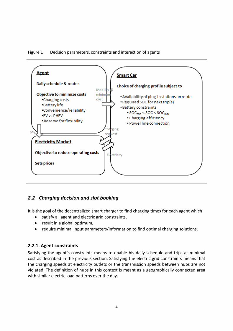
The agent aims to maximize his own utility, e.g. expecting reliable services for his travel and minimizing costs. His boundary conditions which he ideally communicates to the decentra-lized smart charger are his desired driving schedule and routes. The schedule directly relates to the required states of charge (SOCs) for each route and will be passed to the decentra-lized smart charger as the set system constraints. The decentralized smart charger needs to find the optimal charging solution within these constraints which will not violate the technical constraints of the vehicle or the infrastruc-ture, such as the availability of plug-in stations along the route, the battery constraints or the limitations of the power connection. The electric network sets the electricity prices and manages the charging requests of the decentralized smart charger and the various other network loads. Its challenge is to manage the overall energy supplies and demands while keeping the net frequency stable. The pay-ment for its services comes from the agent. In the end, the perfect decentralized smart charger serves the interests of both, the electric-ity producers and the agent: it optimizes the charging processes globally such that the agent’s utility is maximized and violations on the electricity market and thus also operating and maintenance costs are minimized. The parameters described in this section are summarized in Figure 1.
4
Figure 1 Decision parameters, constraints and interaction of agents
2.2 Charging decision and slot booking
It is the goal of the decentralized smart charger to find charging times for each agent which
satisfy all agent and electric grid constraints,
result in a global optimum,
require minimal input parameters/information to find optimal charging solutions.
2.2.1. Agent constraints
Satisfying the agent’s constraints means to enable his daily schedule and trips at minimal cost as described in the previous section. Satisfying the electric grid constraints means that the charging speeds at electricity outlets or the transmission speeds between hubs are not violated. The definition of hubs in this context is meant as a geographically connected area with similar electric load patterns over the day.
5
2.2.2. Global optimum
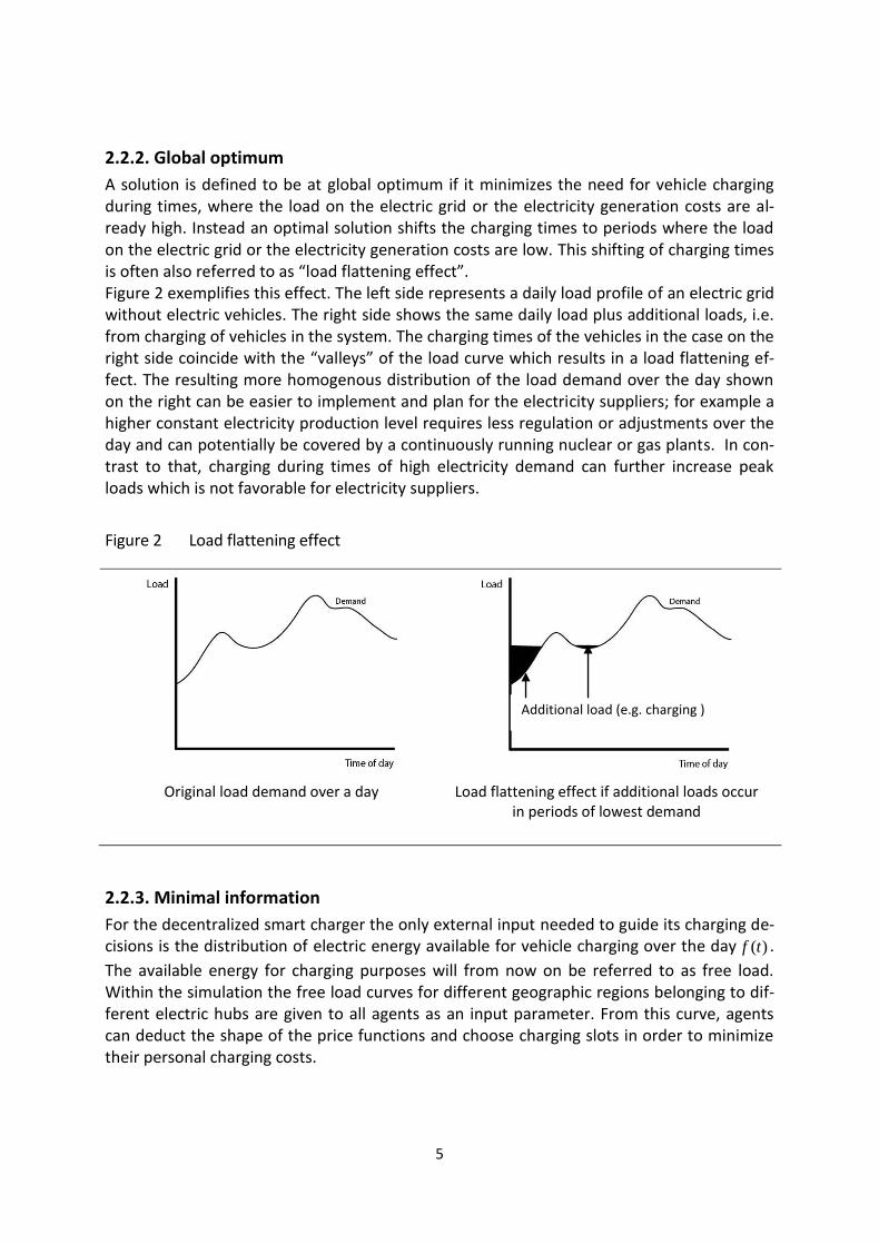
A solution is defined to be at global optimum if it minimizes the need for vehicle charging during times, where the load on the electric grid or the electricity generation costs are al-ready high. Instead an optimal solution shifts the charging times to periods where the load on the electric grid or the electricity generation costs are low. This shifting of charging times is often also referred to as “load flattening effect”. Figure 2 exemplifies this effect. The left side represents a daily load profile of an electric grid without electric vehicles. The right side shows the same daily load plus additional loads, i.e. from charging of vehicles in the system. The charging times of the vehicles in the case on the right side coincide with the “valleys” of the load curve which results in a load flattening ef-fect. The resulting more homogenous distribution of the load demand over the day shown on the right can be easier to implement and plan for the electricity suppliers; for example a higher constant electricity production level requires less regulation or adjustments over the day and can potentially be covered by a continuously running nuclear or gas plants. In con-trast to that, charging during times of high electricity demand can further increase peak loads which is not favorable for electricity suppliers.
Figure 2 Load flattening effect
Original load demand over a day Load flattening effect if additional loads occur in periods of lowest demand
2.2.3. Minimal information
For the decentralized smart charger the only external input needed to guide its charging de-cisions is the distribution of electric energy available for vehicle charging over the day )(tf .
The available energy for charging purposes will from now on be referred to as free load. Within the simulation the free load curves for different geographic regions belonging to dif-ferent electric hubs are given to all agents as an input parameter. From this curve, agents can deduct the shape of the price functions and choose charging slots in order to minimize their personal charging costs.
Additional load (e.g. charging )
6
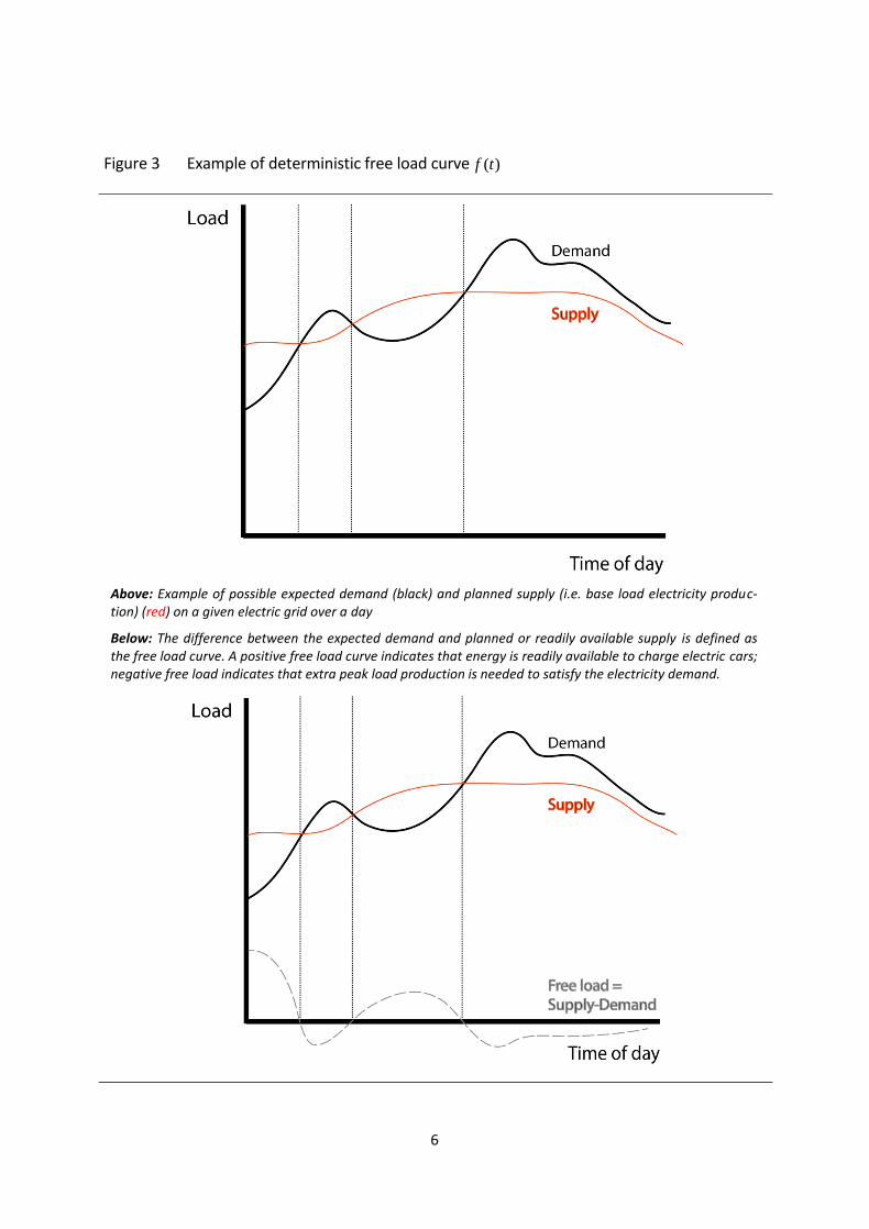
Figure 3 Example of deterministic free load curve )(tf
Above: Example of possible expected demand (black) and planned supply (i.e. base load electricity produc-tion) (red) on a given electric grid over a day
Below: The difference between the expected demand and planned or readily available supply is defined as the free load curve. A positive free load curve indicates that energy is readily available to charge electric cars; negative free load indicates that extra peak load production is needed to satisfy the electricity demand.

7
The definition of free load The free load is defined here as the difference between the possible supply of energy and the actually required amount of energy on the electric grid (see Figure 3). If the free load distribution is positive, free energy is available for charging, if the distribution is negative, charging will result in extra strain on the system. The basic assumptions about the free load curve are that (1) a predictable deterministic part of such a free load curve can be estimated for an existing electric grid (the stochastic part will be dealt with in the V2G section) and (2) this deterministic load curve is recurring or re-mains similar over a period of time, i.e. has a similar profile every day. Thus, it would be suf-ficient to update or synchronize this free load function of the decentralized smart charger only once significant changes of the free load distribution are observed. Deduction of price It is assumed, that the price of charging, )(tp , can be expressed as a function of the free
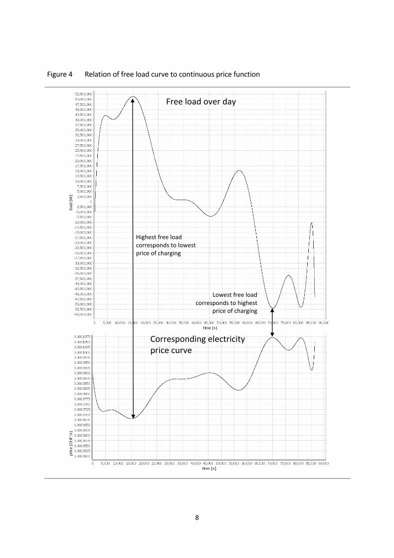
load. The more positive load is available, the cheaper are the charging costs, if the free load is negative, the corresponding costs should be high to discourage agents from charging dur-ing this time. This relation is also described in Appendix A. An example of the relation be-tween free load and the pricing is shown in Figure 4. Time of use pricing, which is commonly used by electricity providers as a measure to influ-ence times of energy consumption, is deliberately avoided. If the price curve is not related to the free load curve one more piece of information would be needed for agents to make the most economic decision. This would complicate the decision process, as the price curve (used to maximize the personal profit) and the load curve (indicating the system optimal so-lution) might be in conflict with each other. Using only one free load curve as the indicator for personal and global utility maximization requires the least number of inputs and offers a coherent basis for the agent’s decision. Free load as probability density function Within the simulation the free load curves for different geographic regions belonging to dif-
ferent electric hubs are given to all agents as an input parameter. From this curve, agents
can deduct the shape of the price functions, as described above, and choose charging slots
in order to optimize the global network. This free load distribution function is used as a
probability density function. In periods with low free load the probability of finding an op-
timal parking spot is small, in periods with great free loads the probability of finding an op-
timal parking spot is larger. Since lower values of a free load curve correspond not only to a
lower probability of finding a spot but also to higher charging costs and large values of the
free load curve correspond to lower charging costs, the proposed system also helps to in-
crease the likelihood of benefitting from the lowest tariffs and thus to increase the likelih-
ood of having low personal charging costs.
The details of this optimization are presented in section 3.
8
Figure 4 Relation of free load curve to continuous price function
Free load over day
Corresponding electricity price curve
Highest free load corresponds to lowest price of charging
Lowest free load corresponds to highest
price of charging
9
2.3. V2G
The potential of V2G charging for frequency control has already been discussed in literature
among others by [7], [8], or [9]. The integration of V2G into the decentralized smart charging
framework now allows to realistically predict potential revenues from V2G for agents for
specific networks and under defined pricing conditions.
2.3.1. The stochastic load
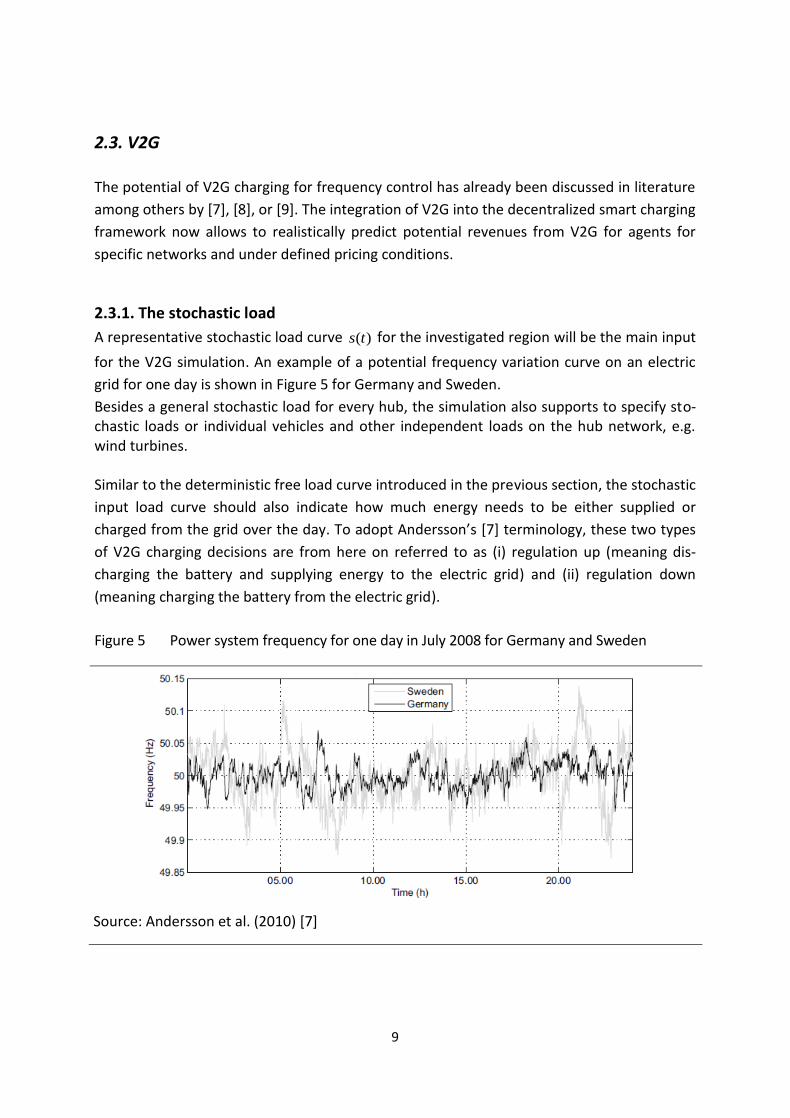
A representative stochastic load curve )(ts for the investigated region will be the main input
for the V2G simulation. An example of a potential frequency variation curve on an electric
grid for one day is shown in Figure 5 for Germany and Sweden.
Besides a general stochastic load for every hub, the simulation also supports to specify sto-chastic loads or individual vehicles and other independent loads on the hub network, e.g. wind turbines. Similar to the deterministic free load curve introduced in the previous section, the stochastic
input load curve should also indicate how much energy needs to be either supplied or
charged from the grid over the day. To adopt Andersson’s [7] terminology, these two types
of V2G charging decisions are from here on referred to as (i) regulation up (meaning dis-
charging the battery and supplying energy to the electric grid) and (ii) regulation down
(meaning charging the battery from the electric grid).
Figure 5 Power system frequency for one day in July 2008 for Germany and Sweden
Source: Andersson et al. (2010) [7]
10
2.3.2. The V2G decision
The decision of agents to provide V2G regulation is dependent on (i) their contract type/their general preference and (ii) on their current state of charge (SOC), (iii) their cur-rent location and (iv) upcoming travel plans. The contract type indicates, if the agent is in general willing to be part of the V2G system. The simulation distinguishes three contract types. (1) Agents who will never provide V2G, (2) agents who will provide regulation down and (3) agents who will provide regulation down and up. Providing regulation down implies cheap charging, whereas regulation up means losing charge which could potentially jeopardize the next journey. Because of the risks asso-ciated with regulation up, it is assumed, that no agent would want a contract with only regu-lation up. The current state of charge is an indicator whether the vehicle is currently available for reg-ulation. If the battery is fully charged, no regulation down can be provided, if the battery is empty no regulation up can be provided. The location determines if the car is currently connected and to which hub. Currently the simulation assumes, that vehicles are plugged whenever they are parking and that every parking spot has the infrastructure for V2G interaction. The charging infrastructure at the lo-cation also determines the limits on the possible (dis)charging speed, i.e. is it a regular con-nection or a speed charging station. Finally, the agent has to decide if providing regulation now will be an economic decision for him. The smart charger compares the expected price of keeping its current charging sche-dule and the price for rescheduling the charging schedule and receiving compensation for its V2G regulation. Only if this rescheduling is possible and if it is not more expensive to re-schedule the charging slots, regulation will be provided (see section 3.3. for a more detailed description).
2.3.3. Optimal solution
Also the V2G decision is supposed to reach an optimal solution, meaning a maximization of the load flattening effect for the stochastic free load, with as few input parameters as possi-ble. It is assumed that vehicles can automatically monitor the frequency on the electric grid with their plug, so that they are informed about the total magnitude of the V2G need in real time,
E . The only missing piece of information for providing V2G is the amount of energy that each vehicle is required to charge. For this, every decentralized smart charger is given a connectivity function )(tc providing information about the average number of parked ve-
hicles as a function of time for every hub. Being able to estimate the number of plugged ve-
hicles, each vehicle can derive the amount of energy, GVE 2 , it is required to charge.
)(
2tc
EE GV
(1)

11
In the proposed system, many small energy sources can pool their capacities together to act on the regulation market. This lowers the entry barrier for providing regulation up and makes it a competitive market. Such pooling already exists today in Germany on the sec-ondary and tertiary regulation market, as long as all energy providers are within the same control area [7]. Accuracy of the connectivity function The success of this procedure is naturally dependent on the accuracy of )(tc . In the best
case, the connectivity function realistically reflects the number of vehicles which are park-ing, connected, willing to provide V2G and able to provide V2G over time. In reality, the number of parking agents would probably be estimated from the known num-ber of registered cars in an area and an aggregated traffic model. If the number of agents is underestimated, the vehicle will try to charge more, if the number of agents is overesti-mated, the agent will charge less than required. Whereas the change in the amount of ener-gy, every agent thinks he needs to charge, in a perfect and an imperfect system can be as-sumed to be quite small per agent, the total V2G energy difference provided over all agents could be more substantial. It remains to be tested, whether inaccurate functions are likely to destabilize the system or whether their effect is likely to be negligible.
12
3. Implementation This section shows how the decentralized charging scheme and V2G are implemented in MATSim building on top of the frameworks and previous work by Waraich et al. [4].
3.1 The simulation framework MATSim
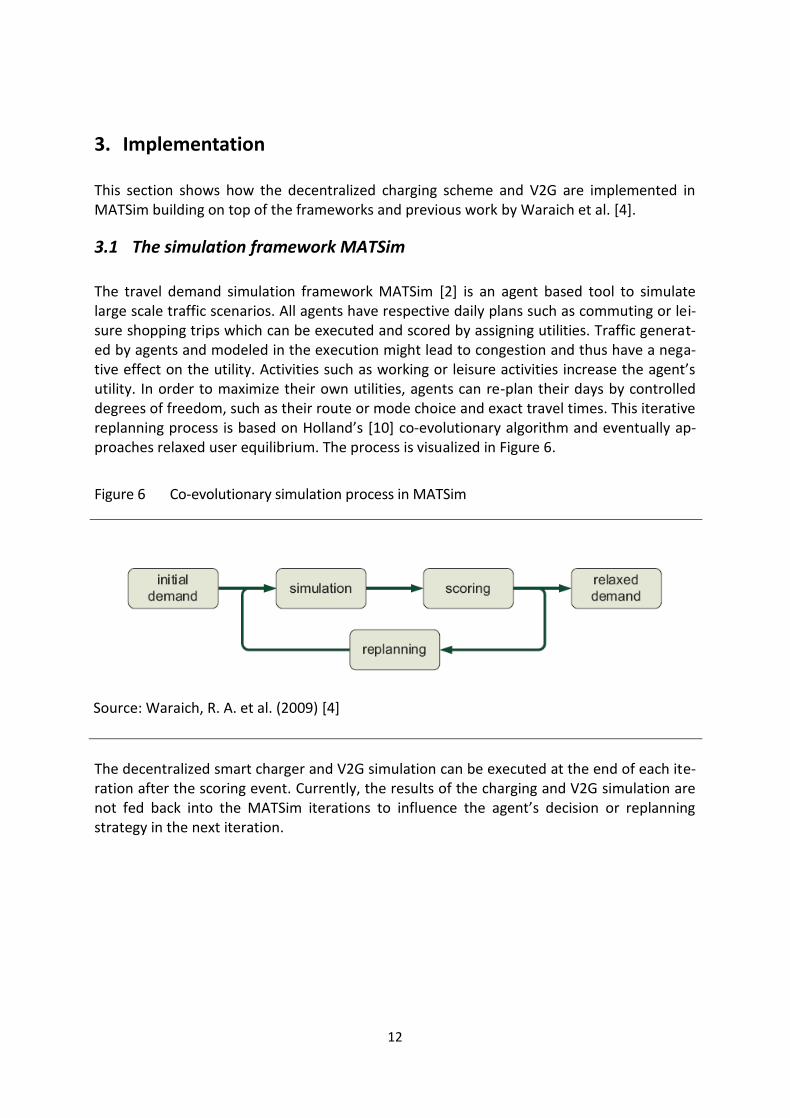
The travel demand simulation framework MATSim [2] is an agent based tool to simulate large scale traffic scenarios. All agents have respective daily plans such as commuting or lei-sure shopping trips which can be executed and scored by assigning utilities. Traffic generat-ed by agents and modeled in the execution might lead to congestion and thus have a nega-tive effect on the utility. Activities such as working or leisure activities increase the agent’s utility. In order to maximize their own utilities, agents can re-plan their days by controlled degrees of freedom, such as their route or mode choice and exact travel times. This iterative replanning process is based on Holland’s [10] co-evolutionary algorithm and eventually ap-proaches relaxed user equilibrium. The process is visualized in Figure 6.
Figure 6 Co-evolutionary simulation process in MATSim
Source: Waraich, R. A. et al. (2009) [4]
The decentralized smart charger and V2G simulation can be executed at the end of each ite-ration after the scoring event. Currently, the results of the charging and V2G simulation are not fed back into the MATSim iterations to influence the agent’s decision or replanning strategy in the next iteration.
13
3.2 The decentralized smart charger
3.2.1. Inputs
The following gives an overview of the essential input parameters for the simulation. An ex-ample input to run the decentralized smart charger in MATSim is presented in Appendix I. Input configuration file: This file is required for any simulation in MATSim and contains in-formation about the simulation, e.g. the network or agent plans input file or the number of iterations to be done1. Output location: This variable specifies the location of the output folder. Electrification rate: The electrification rate defines what percentage of the population owns an EV or PHEV (e.g. 0.8 means 80%). Percentage of EVs: This value defines the percentage of EVs of the total number of electric vehicles in the system (e.g. with an electrification rate of 0.8 and an EV percentage of 50% (=0.5), 40% of the population will own an EV). Hub information: For every hub information on the electricity prices and the available free load need to be given. The minimum and maximum price are defined in the desired currency and the free load in Watt is provided in a 15 minute bin *.txt file. Mapping of Hubs: The existing links within the system need to be mapped to hubs in order to be able to reflect the different prices and free load curves in separate hub areas. (please find more details and a functionality test in Appendix B) Standard charging slot length: The EV or PHEV will try to divide its required charging time within every parking interval into charging slots of a standard charging slot length specified in seconds. Thus, preference is given to multiple shorter charging intervals opposed to fewer very long ones. It is assumed that with smaller intervals the optimization of the charging times will achieve better results, as many small charging intervals might better capture the shape of the free load curve opposed to few long charging slots. Battery buffer for EVs: The battery buffer is a reserve that should be charged by EVs in addi-tion to what the vehicle will be using in its next trip (e.g. a buffer of 0.2 means 20% more energy than required by the next trip should be stored in the battery right before the trip).
1 for more information please look at the tutorials on http://matsim.org
14
3.2.2. Outputs
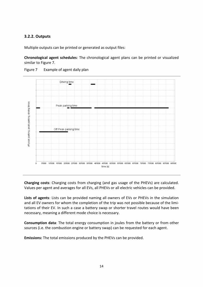
Multiple outputs can be printed or generated as output files: Chronological agent schedules: The chronological agent plans can be printed or visualized similar to Figure 7.
Figure 7 Example of agent daily plan
Charging costs: Charging costs from charging (and gas usage of the PHEVs) are calculated. Values per agent and averages for all EVs, all PHEVs or all electric vehicles can be provided. Lists of agents: Lists can be provided naming all owners of EVs or PHEVs in the simulation and all EV owners for whom the completion of the trip was not possible because of the limi-tations of their EV. In such a case a battery swap or shorter travel routes would have been necessary, meaning a different mode choice is necessary. Consumption data: The total energy consumption in joules from the battery or from other sources (i.e. the combustion engine or battery swap) can be requested for each agent. Emissions: The total emissions produced by the PHEVs can be provided.
15
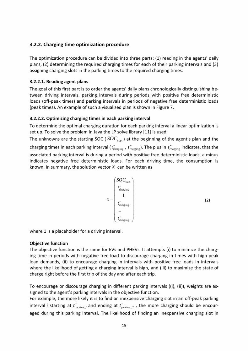
3.2.2. Charging time optimization procedure
The optimization procedure can be divided into three parts: (1) reading in the agents’ daily plans, (2) determining the required charging times for each of their parking intervals and (3) assigning charging slots in the parking times to the required charging times.
3.2.2.1. Reading agent plans
The goal of this first part is to order the agents’ daily plans chronologically distinguishing be-tween driving intervals, parking intervals during periods with positive free deterministic loads (off-peak times) and parking intervals in periods of negative free deterministic loads (peak times). An example of such a visualized plan is shown in Figure 7.
3.2.2.2. Optimizing charging times in each parking interval
To determine the optimal charging duration for each parking interval a linear optimization is set up. To solve the problem in Java the LP solve library [11] is used.
The unknowns are the starting SOC ( startSOC ) at the beginning of the agent’s plan and the
charging times in each parking interval (
chargingt ,
chargingt ). The plus in
chargingt
indicates, that the
associated parking interval is during a period with positive free deterministic loads, a minus indicates negative free deterministic loads. For each driving time, the consumption is known. In summary, the solution vector x can be written as
charging
charging
charging
start
...
1
t
t
t
SOC
x (2)
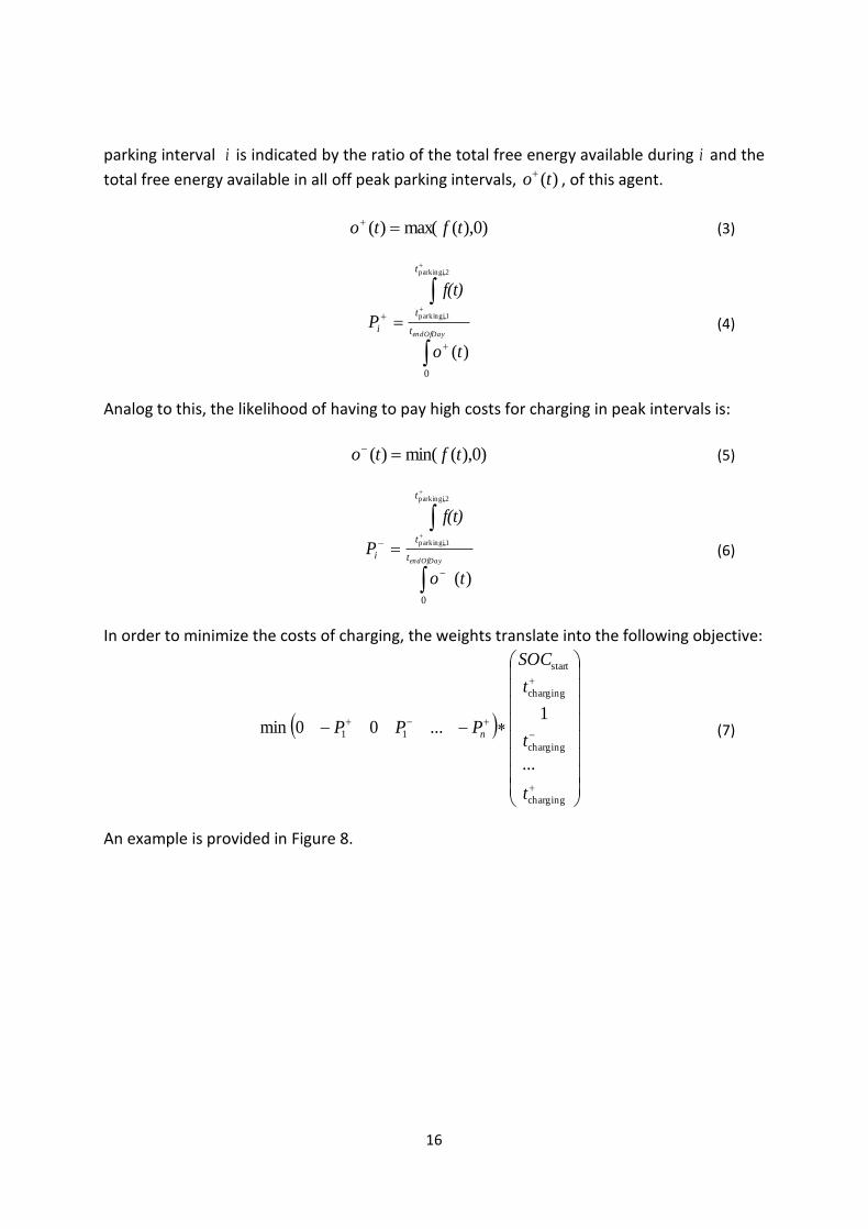
where 1 is a placeholder for a driving interval. Objective function The objective function is the same for EVs and PHEVs. It attempts (i) to minimize the charg-ing time in periods with negative free load to discourage charging in times with high peak load demands, (ii) to encourage charging in intervals with positive free loads in intervals where the likelihood of getting a charging interval is high, and (iii) to maximize the state of charge right before the first trip of the day and after each trip. To encourage or discourage charging in different parking intervals ((i), (ii)), weights are as-signed to the agent’s parking intervals in the objective function. For example, the more likely it is to find an inexpensive charging slot in an off-peak parking
interval i
starting at
i,1parking,t and ending at
i,2parking,t , the more charging should be encour-
aged during this parking interval. The likelihood of finding an inexpensive charging slot in
16
parking interval i
is indicated by the ratio of the total free energy available during i
and the
total free energy available in all off peak parking intervals, )(to , of this agent.
)0),(max()( tfto (3)
endOfDayt
t
t
i
to
f(t)
P
0
)(
i,2parking,
i,1parking,
(4)
Analog to this, the likelihood of having to pay high costs for charging in peak intervals is:
)0),(min()( tfto (5)
endOfDayt
t
t
i
to
f(t)
P
0
)(
i,2parking,
i,1parking,
(6)
In order to minimize the costs of charging, the weights translate into the following objective:
charging
charging
charging
start
11
...
100min
t
t
t
SOC
P...PP n (7)
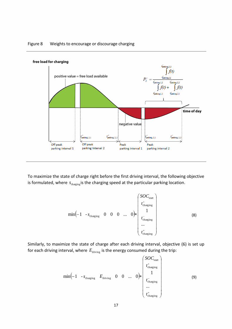
An example is provided in Figure 8.
17
Figure 8 Weights to encourage or discourage charging
To maximize the state of charge right before the first driving interval, the following objective
is formulated, where chargings is the charging speed at the particular parking location.
charging
charging
charging
start
charging
...
10...000- 1min
t
t
t
SOC
s (8)
Similarly, to maximize the state of charge after each driving interval, objective (6) is set up
for each driving interval, where drivingE
is the energy consumed during the trip:
charging
charging
charging
start
drivingcharging
...
10...00-1min
t
t
t
SOC
Es (9)
18
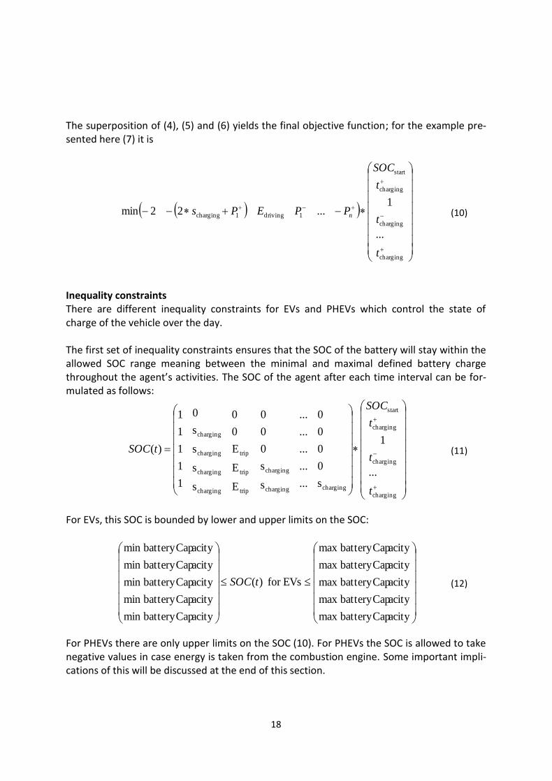
The superposition of (4), (5) and (6) yields the final objective function; for the example pre-sented here (7) it is
charging
charging
charging
start
1driving1charging
...
1...22min
t
t
t
SOC
PPEPs n (10)
Inequality constraints There are different inequality constraints for EVs and PHEVs which control the state of charge of the vehicle over the day. The first set of inequality constraints ensures that the SOC of the battery will stay within the allowed SOC range meaning between the minimal and maximal defined battery charge throughout the agent’s activities. The SOC of the agent after each time interval can be for-mulated as follows:
charging
charging
charging
start
chargingcharging
charging
trip
trip
trip
charging
charging
charging
charging
...
1
s
0
0
0
0
...
...
...
...
...
s
s
0
0
0
E
E
E
0
0
s
s
s
s
0
1
1
1
1
1
)(
t
t
t
SOC
tSOC (11)
For EVs, this SOC is bounded by lower and upper limits on the SOC:
acitybatteryCapmax
acitybatteryCapmax
acitybatteryCapmax
acitybatteryCapmax
acitybatteryCapmax
EVsfor )(
acitybatteryCapmin
acitybatteryCapmin
acitybatteryCapmin
acitybatteryCapmin
acitybatteryCapmin
tSOC (12)
For PHEVs there are only upper limits on the SOC (10). For PHEVs the SOC is allowed to take negative values in case energy is taken from the combustion engine. Some important impli-cations of this will be discussed at the end of this section.
19
acitybatteryCapmax
acitybatteryCapmax
acitybatteryCapmax
acitybatteryCapmax
acitybatteryCapmax
PHEVsfor )(tSOC (13)
This setup does not simulate a recurring day routine with the same starting and end SOC
every day. Originally, the author had imposed an equality constraint to limit the charged
energy to the actual energy need [6]. Realizing that this might be an unrealistic assumption
because agents will probably prefer to recharge their batteries fully whenever possible, this
is changed in this thesis.
The second type of inequality constraints only applies to EVs. A buffer can be defined which
is the minimum battery reserve the car needs to have in addition to the expected energy
consumption of the next trip before starting a new trip. Since the SOC of PHEVs can fall be-
low zero, such a buffer is not implemented for PHEVs. (11) exemplifies how to enforce that the EV has at least the required buffer before its trip:
buffer1
...
10...001 driving
charging
charging
charging
start
charging
E
t
t
t
SOC
s (14)
Upper and lower bounds The upper and lower bounds restrict the solution space for the battery’s state of charge and for the charging times to realistic values. The starting state of charge is required to remain within the battery’s defined minimum and maximum charge. Charging times can only be
positive and cannot be greater than the total duration of the parking interval, parkingt . Again,
for driving times the lower and upper bounds correspond to the 1 as a placeholder.
20
parking
parking
parking
charging
charging
charging
start
...
1
maxChargeSizebattery
...
1x
0
...0
1
0
minChargeSizebattery
t
t
t
t
t
t
SOC
(15)
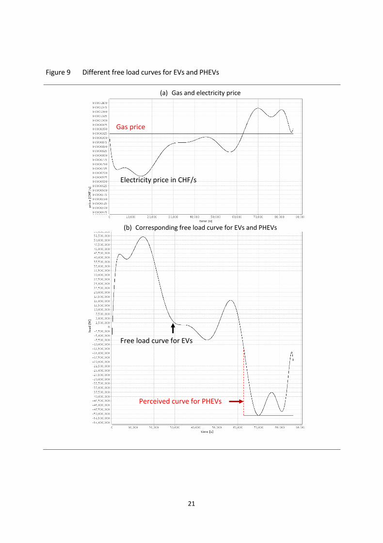
More on PHEVs and EVs Accounting for the gas price Beside the slight differences in the set up of the optimization there is one more way, the si-mulation distinguishes between EVs and PHEVs. Since PHEVs have two possible fuel options (using electricity from their battery or using gas), PHEVs should never charge at times, where the cost of charging electricity is greater than the cost of gas. To ensure that the weights assigned in the optimization reflect this preference, PHEVs use an indicator function different from the load curve which has extremely high negative values in intervals where using gas is the economic choice. Figure 9-a gives an overview of charging and gas costs (US price) over the day. Figure 9-b shows the corresponding free load curve for EVs in black and the perceived curve for PHEVs in red. (please see Appendix E for more details)
21
Figure 9 Different free load curves for EVs and PHEVs
(a) Gas and electricity price
(b) Corresponding free load curve for EVs and PHEVs
Gas price
Electricity price in CHF/s
Free load curve for EVs
Perceived curve for PHEVs
22
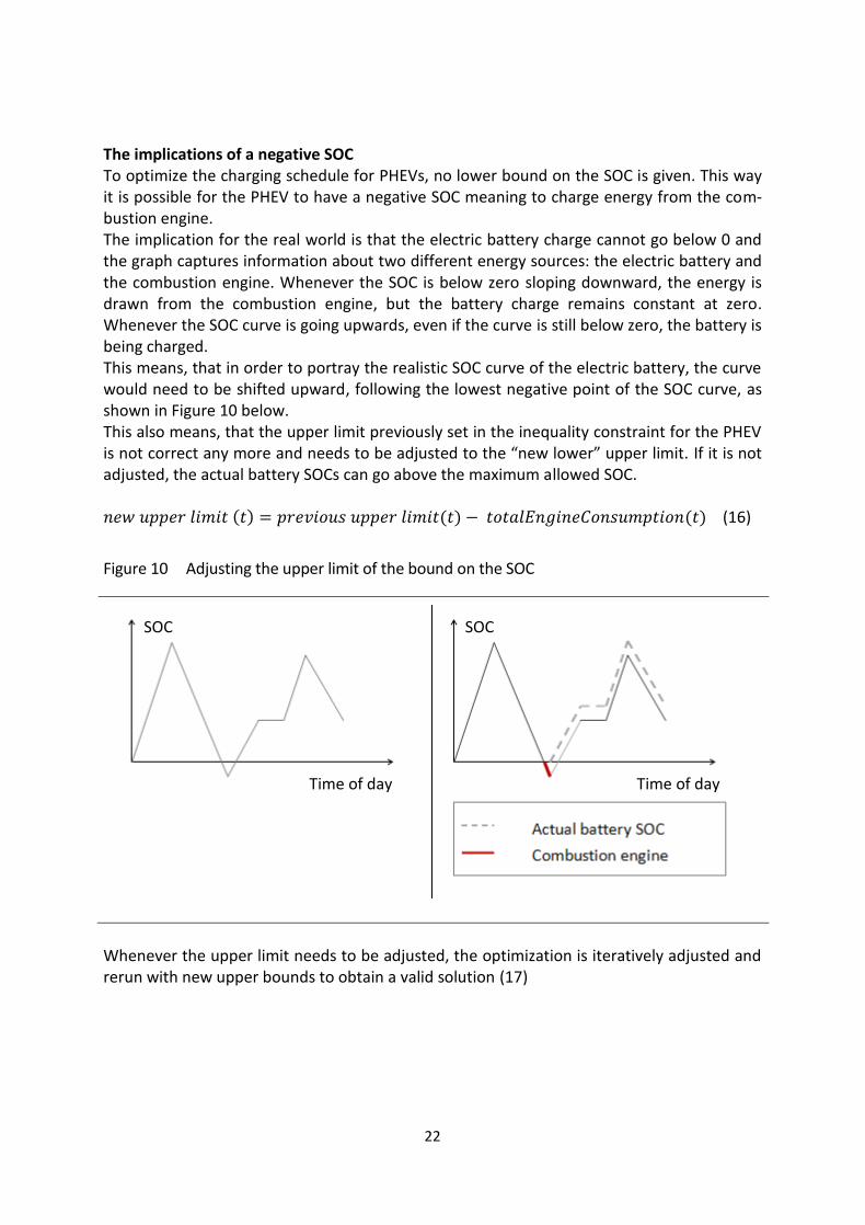
The implications of a negative SOC To optimize the charging schedule for PHEVs, no lower bound on the SOC is given. This way it is possible for the PHEV to have a negative SOC meaning to charge energy from the com-bustion engine. The implication for the real world is that the electric battery charge cannot go below 0 and the graph captures information about two different energy sources: the electric battery and the combustion engine. Whenever the SOC is below zero sloping downward, the energy is drawn from the combustion engine, but the battery charge remains constant at zero. Whenever the SOC curve is going upwards, even if the curve is still below zero, the battery is being charged. This means, that in order to portray the realistic SOC curve of the electric battery, the curve would need to be shifted upward, following the lowest negative point of the SOC curve, as shown in Figure 10 below. This also means, that the upper limit previously set in the inequality constraint for the PHEV is not correct any more and needs to be adjusted to the “new lower” upper limit. If it is not adjusted, the actual battery SOCs can go above the maximum allowed SOC. (16)
Figure 10 Adjusting the upper limit of the bound on the SOC
Whenever the upper limit needs to be adjusted, the optimization is iteratively adjusted and rerun with new upper bounds to obtain a valid solution (17)
Time of day Time of day
SOC SOC
23
(t)limit upper new
(t)limit upper new
(t)limit upper new
(t)limit upper new
(t)limit upper new
PHEVsfor )(tSOC
(17)
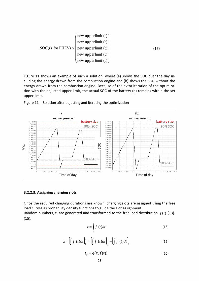
Figure 11 shows an example of such a solution, where (a) shows the SOC over the day in-cluding the energy drawn from the combustion engine and (b) shows the SOC without the energy drawn from the combustion engine. Because of the extra iteration of the optimiza-tion with the adjusted upper limit, the actual SOC of the battery (b) remains within the set upper limit.
Figure 11 Solution after adjusting and iterating the optimization
(a) (b)
3.2.2.3. Assigning charging slots
Once the required charging durations are known, charging slots are assigned using the free load curves as probability density functions to guide the slot assignment. Random numbers, z, are generated and transformed to the free load distribution )(tf (13)-
(15).
xt
o
dttfz )( (18)
00
)()()( dttfdttfdttfzx
x
t
t
(19)
))(,( tfzgtx (20)
battery size battery size
Time of day
10% SOC 10% SOC
90% SOC
Time of day
SOC
SOC
90% SOC

24
Updating the new free load curve To evaluate the effect of the charging activities on the load curve of the electric grid, the free load curve is updated at the end of the simulation. For performance reasons, the updated curve is only stored in the form of aggregated data points and not as continuous functions.
25
3.3 The V2G procedure
3.3.1. Inputs
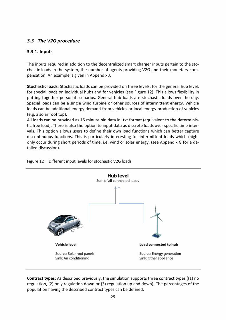
The inputs required in addition to the decentralized smart charger inputs pertain to the sto-chastic loads in the system, the number of agents providing V2G and their monetary com-pensation. An example is given in Appendix J. Stochastic loads: Stochastic loads can be provided on three levels: for the general hub level, for special loads on individual hubs and for vehicles (see Figure 12). This allows flexibility in putting together personal scenarios. General hub loads are stochastic loads over the day. Special loads can be a single wind turbine or other sources of intermittent energy. Vehicle loads can be additional energy demand from vehicles or local energy production of vehicles (e.g. a solar roof top). All loads can be provided as 15 minute bin data in .txt format (equivalent to the determinis-tic free load). There is also the option to input data as discrete loads over specific time inter-vals. This option allows users to define their own load functions which can better capture discontinuous functions. This is particularly interesting for intermittent loads which might only occur during short periods of time, i.e. wind or solar energy. (see Appendix G for a de-tailed discussion).
Figure 12 Different input levels for stochastic V2G loads
Contract types: As described previously, the simulation supports three contract types ((1) no regulation, (2) only regulation down or (3) regulation up and down). The percentages of the population having the described contract types can be defined.
26
Compensation: Monetary rewards can be defined and are specified in CHF per kWh. Such V2G services can include (i) regulation up and down of vehicles, and (ii) feed-in tariffs for wind turbines or other energy producers connected to the grid.
3.3.2. Outputs
Revenue: The revenue per agent and the average revenues for EVs, PHEVs from V2G servic-es and feed-in can be provided. Total and average regulation energy: The total and average energy provided for regulation up and down for EVs, PHEVs and all vehicles can be requested.
3.3.3. Procedure
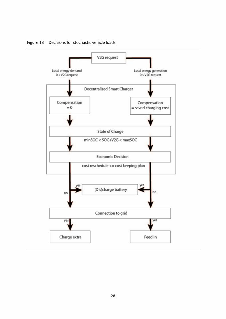
The V2G simulation has three parts: (1) adjusting the stochastic hub load with the stochastic vehicle loads, (2) adjusting stochastic hub load with stochastic hub sources in the system and (3) checking all remaining stochastic hub loads. Stochastic vehicle loads In the first part, the simulation will check the stochastic vehicle loads. If the load is positive, meaning it is a local energy production, the simulation will try to charge the battery with the available energy. If this is not possible and if the vehicle is connected to the grid at this point in time, the superfluous energy will be fed into the electric grid and added to the stochastic hub load distribution. For any additional local battery load, the simulation will attempt to pull the requested charge from the battery. If this is not possible, additional energy will be charged from the electric grid to satisfy the energy demand in case the vehicle is connected. To decide if the (dis)charging decision is economic, the costs between keeping the current schedule and rescheduling are compared. To calculate the costs of rescheduling, the reward for (dis)charging is taken into account. The reward in the case of charging the battery from local energy production is equal to the charging costs saved. For discharging the battery to provide energy for a local vehicle load, i.e. turning on the radio or air conditioning, the agent does not receive any external compensation and the compensation is zero. This decision tree is presented in Figure 13.

27
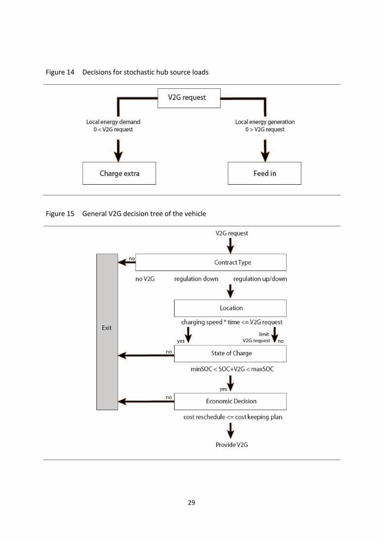
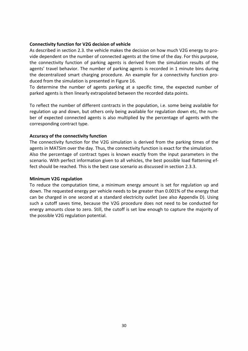
Stochastic hub sources The stochastic hub sources, for example wind turbines or solar roofs, are assumed to be permanently connected to the grid at a fixed location. Thus, if they generate energy, the energy can always be fed into the system. In case they require extra energy, if they are a negative source or “sink”, it will be charged from the electric grid. Since they do not have their own optimized schedule or their own battery associated with them, no economic checks apply here. This decision tree is presented in Figure 14. V2G with the remaining hub load To check the availability of vehicles for V2G services for the hub loads, the remaining sto-chastic load (the hub load after steps (1) and (2)) is calculated (details can be found in Ap-pendix C). Then, the simulation follows the scheme presented in Figure 15 which was pre-viously outlined in section 2.3. to decide whether a vehicle is available for V2G.
28
Figure 13 Decisions for stochastic vehicle loads
29
Figure 14 Decisions for stochastic hub source loads
Figure 15 General V2G decision tree of the vehicle
30
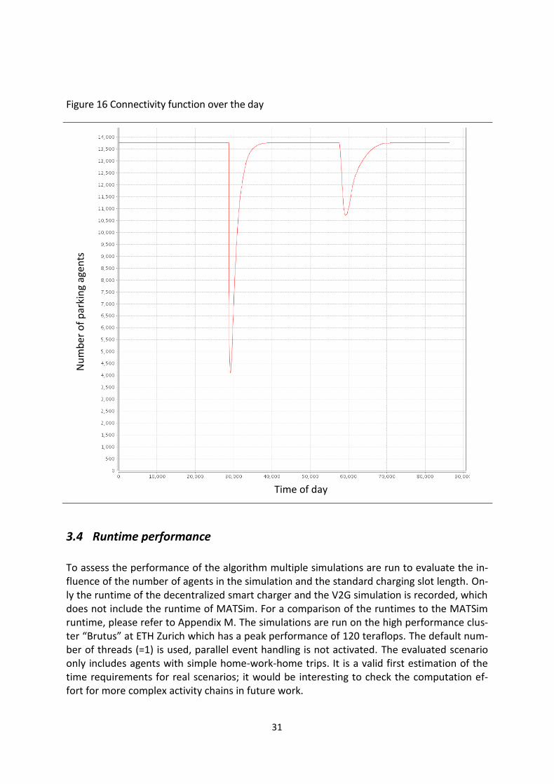
Connectivity function for V2G decision of vehicle As described in section 2.3. the vehicle makes the decision on how much V2G energy to pro-vide dependent on the number of connected agents at the time of the day. For this purpose, the connectivity function of parking agents is derived from the simulation results of the agents’ travel behavior. The number of parking agents is recorded in 1 minute bins during the decentralized smart charging procedure. An example for a connectivity function pro-duced from the simulation is presented in Figure 16. To determine the number of agents parking at a specific time, the expected number of parked agents is then linearly extrapolated between the recorded data points. To reflect the number of different contracts in the population, i.e. some being available for regulation up and down, but others only being available for regulation down etc, the num-ber of expected connected agents is also multiplied by the percentage of agents with the corresponding contract type. Accuracy of the connectivity function The connectivity function for the V2G simulation is derived from the parking times of the agents in MATSim over the day. Thus, the connectivity function is exact for the simulation. Also the percentage of contract types is known exactly from the input parameters in the scenario. With perfect information given to all vehicles, the best possible load flattening ef-fect should be reached. This is the best case scenario as discussed in section 2.3.3. Minimum V2G regulation To reduce the computation time, a minimum energy amount is set for regulation up and down. The requested energy per vehicle needs to be greater than 0.001% of the energy that can be charged in one second at a standard electricity outlet (see also Appendix D). Using such a cutoff saves time, because the V2G procedure does not need to be conducted for energy amounts close to zero. Still, the cutoff is set low enough to capture the majority of the possible V2G regulation potential.
31
Figure 16 Connectivity function over the day
3.4 Runtime performance
To assess the performance of the algorithm multiple simulations are run to evaluate the in-fluence of the number of agents in the simulation and the standard charging slot length. On-ly the runtime of the decentralized smart charger and the V2G simulation is recorded, which does not include the runtime of MATSim. For a comparison of the runtimes to the MATSim runtime, please refer to Appendix M. The simulations are run on the high performance clus-ter “Brutus” at ETH Zurich which has a peak performance of 120 teraflops. The default num-ber of threads (=1) is used, parallel event handling is not activated. The evaluated scenario only includes agents with simple home-work-home trips. It is a valid first estimation of the time requirements for real scenarios; it would be interesting to check the computation ef-fort for more complex activity chains in future work.
Nu
mb
er o
f p
arki
ng
agen
ts
Time of day
32
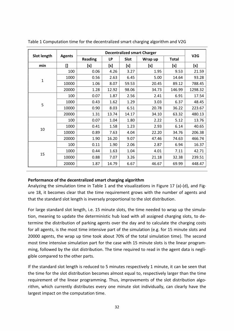
Table 1 Computation time for the decentralized smart charging algorithm and V2G
Slot length Agents Decentralized smart Charger
V2G Reading LP Slot Wrap up Total
min [] [s] [s] [s] [s] [s] [s]
1
100 0.06 4.26 3.27 1.95 9.53 21.59
1000 0.56 2.63 6.45 5.00 14.64 93.28
10000 1.06 8.07 59.53 20.45 89.12 788.45
20000 1.28 12.92 98.06 34.73 146.99 1298.32
5
100 0.07 1.87 2.56 2.41 6.91 17.54
1000 0.43 1.62 1.29 3.03 6.37 48.45
10000 0.90 8.03 6.51 20.78 36.22 223.67
20000 1.31 13.74 14.17 34.10 63.32 480.13
10
100 0.07 1.04 1.80 2.22 5.12 13.76
1000 0.41 1.58 1.23 2.93 6.14 40.65
10000 0.89 7.63 4.04 22.20 34.76 206.38
20000 1.90 16.20 9.07 47.46 74.63 466.74
15
100 0.11 1.90 2.06 2.87 6.94 16.37
1000 0.44 1.63 1.04 4.01 7.11 42.71
10000 0.88 7.07 3.26 21.18 32.38 239.51
20000 1.87 14.79 6.67 46.67 69.99 448.47
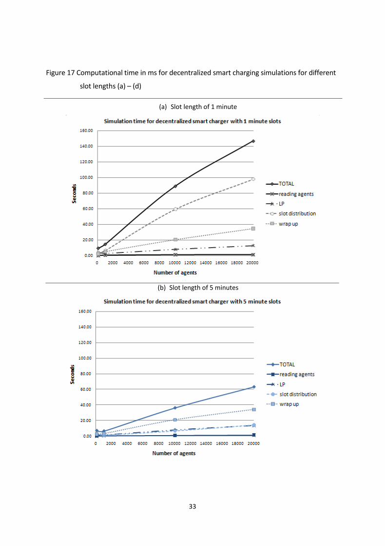
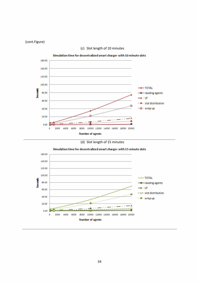
Performance of the decentralized smart charging algorithm Analyzing the simulation time in Table 1 and the visualizations in Figure 17 (a)-(d), and Fig-
ure 18, it becomes clear that the time requirement grows with the number of agents and
that the standard slot length is inversely proportional to the slot distribution.
For large standard slot length, i.e. 15 minute slots, the time needed to wrap up the simula-
tion, meaning to update the deterministic hub load with all assigned charging slots, to de-
termine the distribution of parking agents over the day and to calculate the charging costs
for all agents, is the most time intensive part of the simulation (e.g. for 15 minute slots and
20000 agents, the wrap up time took about 70% of the total simulation time). The second
most time intensive simulation part for the case with 15 minute slots is the linear program-
ming, followed by the slot distribution. The time required to read in the agent data is negli-
gible compared to the other parts.
If the standard slot length is reduced to 5 minutes respectively 1 minute, it can be seen that
the time for the slot distribution becomes almost equal to, respectively larger than the time
requirement of the linear programming. Thus, improvements of the slot distribution algo-
rithm, which currently distributes every one minute slot individually, can clearly have the
largest impact on the computation time.
33
Figure 17 Computational time in ms for decentralized smart charging simulations for different
slot lengths (a) – (d)
(a) Slot length of 1 minute
(b) Slot length of 5 minutes
34
(cont.Figure)
(c) Slot length of 10 minutes
(d) Slot length of 15 minutes
35
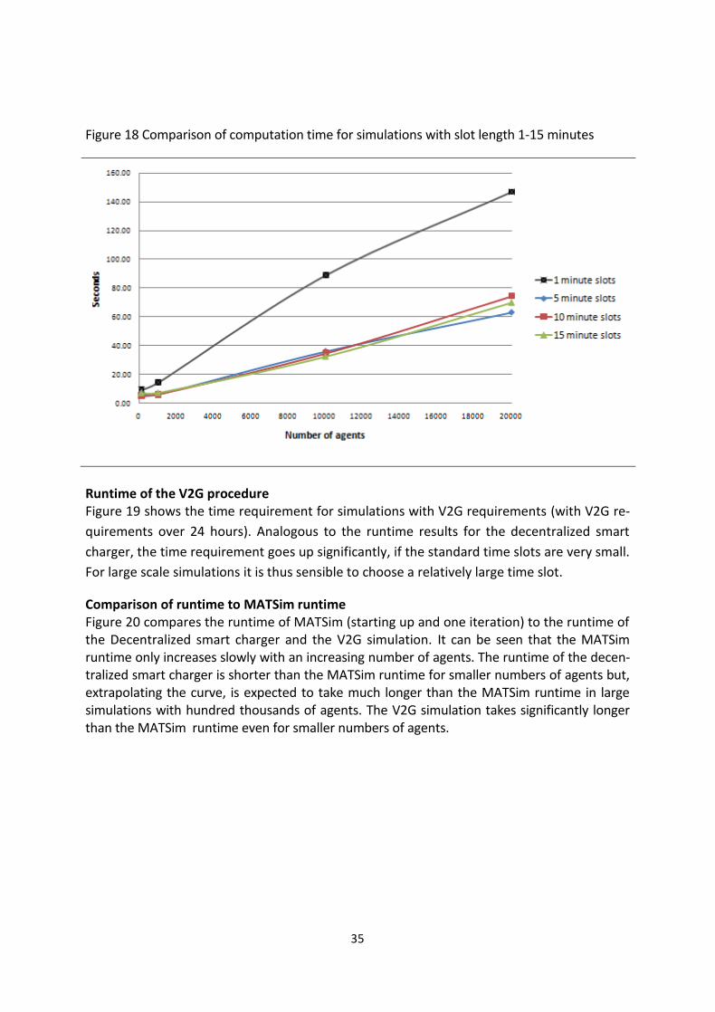
Figure 18 Comparison of computation time for simulations with slot length 1-15 minutes
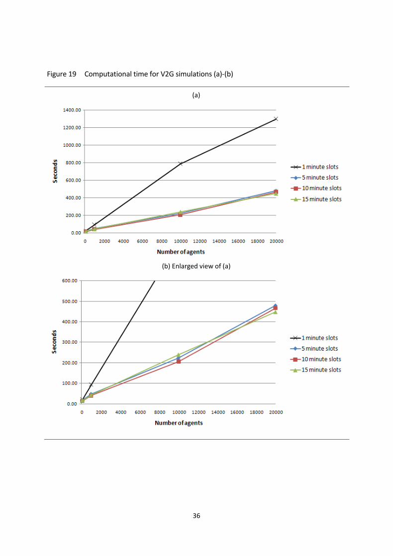
Runtime of the V2G procedure Figure 19 shows the time requirement for simulations with V2G requirements (with V2G re-
quirements over 24 hours). Analogous to the runtime results for the decentralized smart
charger, the time requirement goes up significantly, if the standard time slots are very small.
For large scale simulations it is thus sensible to choose a relatively large time slot.
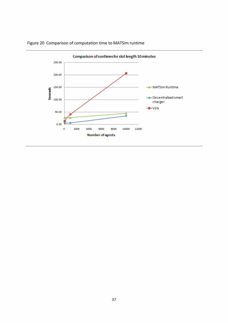
Comparison of runtime to MATSim runtime Figure 20 compares the runtime of MATSim (starting up and one iteration) to the runtime of the Decentralized smart charger and the V2G simulation. It can be seen that the MATSim runtime only increases slowly with an increasing number of agents. The runtime of the decen-tralized smart charger is shorter than the MATSim runtime for smaller numbers of agents but, extrapolating the curve, is expected to take much longer than the MATSim runtime in large simulations with hundred thousands of agents. The V2G simulation takes significantly longer than the MATSim runtime even for smaller numbers of agents.
36
Figure 19 Computational time for V2G simulations (a)-(b)
(a)
(b) Enlarged view of (a)
37
Figure 20 Comparison of computation time to MATSim runtime
38
4. Simulations
4.1. Assessing the influence of EVs, prices, battery sizes and contract types on the system
A set of simulations was run to analyze the influence of
the ratio of EVs to PHEVs in the system
the price of gas
the percentage of people providing regulation up and down opposed to only regula-tion down and
the battery size on the behavior and performance of the agents. Relevant output variables are the ability of vehicles to finish their trips, the charging duration, emissions, costs, and revenues. The simu-lation results are also used to evaluate the functionality of the decentralized smart charger and the V2G procedure. For this purpose a full factorial design is set up with the factors and levels shown in Table 2: Table 2 Computational Time for the decentralized smart charging algorithm and V2G Levels
Factor 1 2 3 4
EV Penetration 10% 25% 75% 90%
Price of gas US price CH price - -
% of providing regulation up & down 0% 33% 67% 100%
battery size 16kWh 24kWh - -
A full factorial design is preferred over a fractional factorial design, to be able to not only es-timate the effect of every single variable on the system, but also to be able to completely plot solution surfaces to better visualize and understand the behavior of the system.
4.1.1. Input parameters and setup
Network The simulation was run using the Berlin test scenario of the Institute for Transport Planning and Systems which comprises a 1% population sample of 16.000 agents and home-work-home and home-education-home trips. The network is modeled as one single hub. Free deterministic load The used free load curve was derived from a typical residential load profile (Figure 21).
39
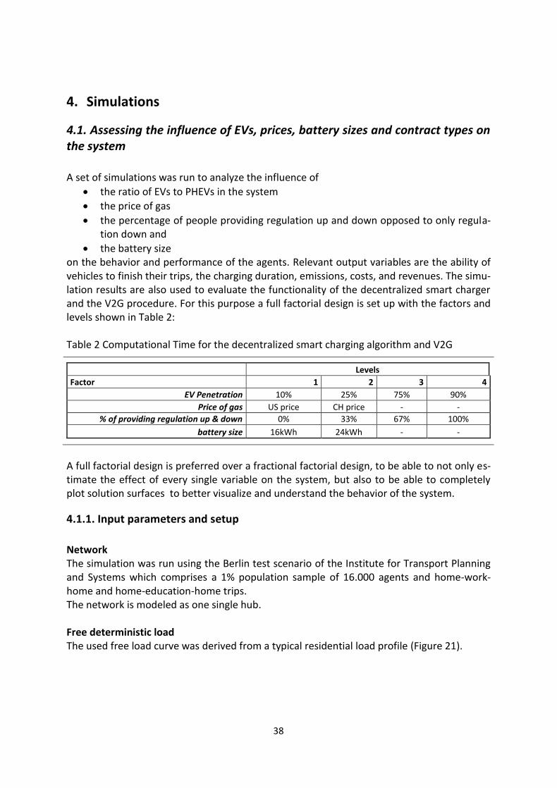
Figure 21 Derivation of free load curve from typical residential load profile
First, the residential load profile (black) is fitted to a polynomial function (red dashed). To generate the free load curve, it is assumed that a constant base energy production is possi-ble at 85% of the peak of the residential load profile (grey). The resulting difference between the assumed base energy production and the fitted load profile is taken as the basic shape of an initial guess free load curve (red). The free load curve is then modified for the Berlin scenario, such that enough energy can be provided for the number of agents in the simulation in all run simulations. Thus, the free load curve is scaled such that the sum of the integrals, in those ranges where the domain is positive g(x) (16), is not less than the total energy demand of all electric vehicles (17). )0),(max()( xfxg (21)
demandenergy total)( xg (22)
40
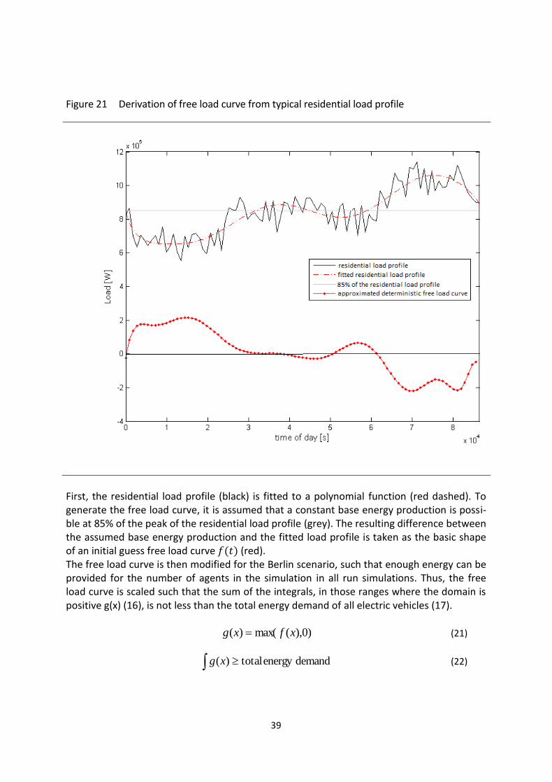
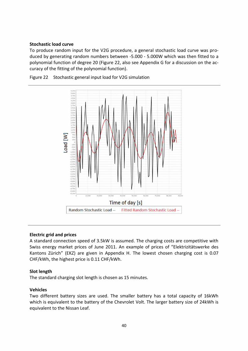
Stochastic load curve To produce random input for the V2G procedure, a general stochastic load curve was pro-duced by generating random numbers between -5.000 - 5.000W which was then fitted to a polynomial function of degree 20 (Figure 22, also see Appendix G for a discussion on the ac-curacy of the fitting of the polynomial function).
Figure 22 Stochastic general input load for V2G simulation
Electric grid and prices A standard connection speed of 3.5kW is assumed. The charging costs are competitive with Swiss energy market prices of June 2011. An example of prices of “Elektrizitätswerke des Kantons Zürich” (EKZ) are given in Appendix H. The lowest chosen charging cost is 0.07 CHF/kWh, the highest price is 0.11 CHF/kWh. Slot length The standard charging slot length is chosen as 15 minutes. Vehicles Two different battery sizes are used. The smaller battery has a total capacity of 16kWh which is equivalent to the battery of the Chevrolet Volt. The larger battery size of 24kWh is equivalent to the Nissan Leaf.
41
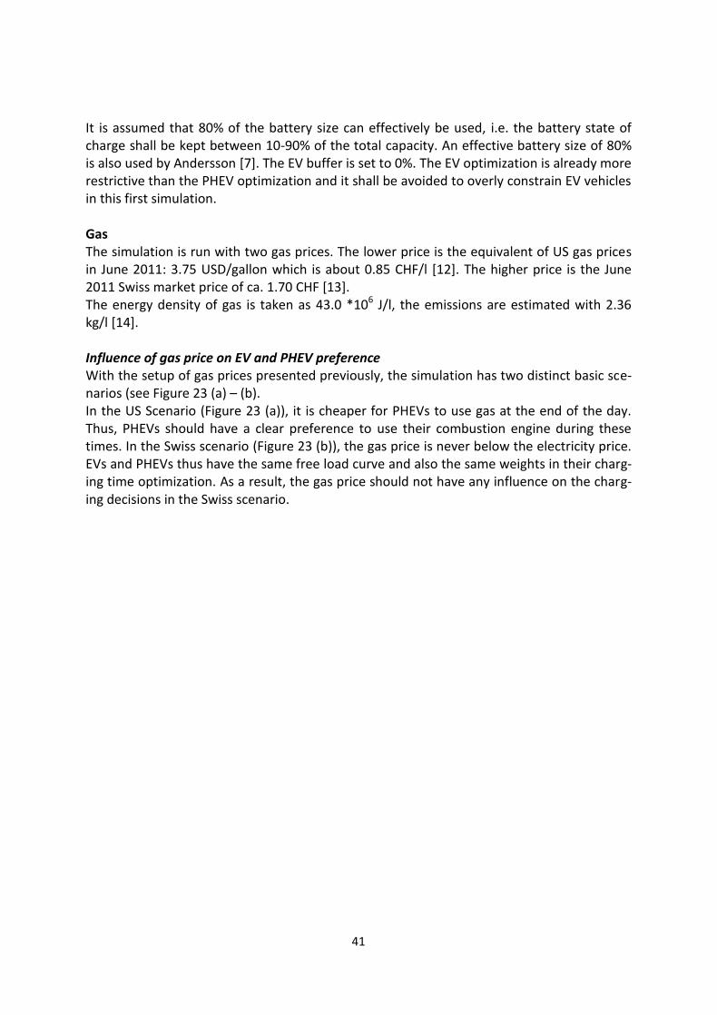
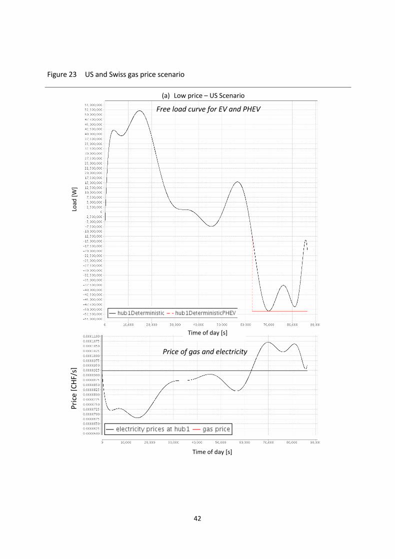
It is assumed that 80% of the battery size can effectively be used, i.e. the battery state of charge shall be kept between 10-90% of the total capacity. An effective battery size of 80% is also used by Andersson [7]. The EV buffer is set to 0%. The EV optimization is already more restrictive than the PHEV optimization and it shall be avoided to overly constrain EV vehicles in this first simulation. Gas The simulation is run with two gas prices. The lower price is the equivalent of US gas prices in June 2011: 3.75 USD/gallon which is about 0.85 CHF/l [12]. The higher price is the June 2011 Swiss market price of ca. 1.70 CHF [13]. The energy density of gas is taken as 43.0 *106 J/l, the emissions are estimated with 2.36 kg/l [14]. Influence of gas price on EV and PHEV preference With the setup of gas prices presented previously, the simulation has two distinct basic sce-narios (see Figure 23 (a) – (b). In the US Scenario (Figure 23 (a)), it is cheaper for PHEVs to use gas at the end of the day. Thus, PHEVs should have a clear preference to use their combustion engine during these times. In the Swiss scenario (Figure 23 (b)), the gas price is never below the electricity price. EVs and PHEVs thus have the same free load curve and also the same weights in their charg-ing time optimization. As a result, the gas price should not have any influence on the charg-ing decisions in the Swiss scenario.
42
Figure 23 US and Swiss gas price scenario
(a) Low price – US Scenario
Free load curve for EV and PHEV
Price of gas and electricity
Load
[W
]
Pri
ce [
CH
F/s]
Time of day [s]
Time of day [s]
43
(b) Large price – Swiss scenario
Free load curve for EV and PHEV
Price of gas and electricity
Load
[W
]
Pri
ce [
CH
F/s]
Time of day [s]
Time of day [s]
44
4.2. Additional tests
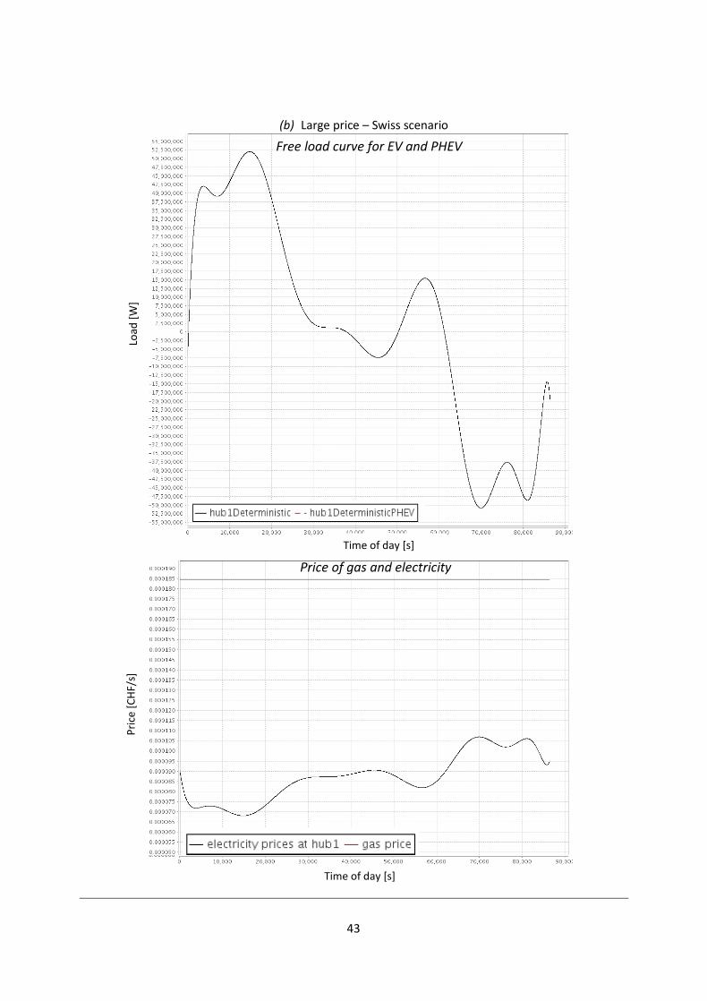
4.2.1. V2G Saturation limit
To explore how much V2G regulation the vehicles could provide up and down maximally,
additional simulations are run
adjusting the stochastic input curve
increasing the compensation level for V2G regulation
Two scenarios are run with constant input curves of constant +50.000W or -50.000 W over
the entire day. The negative load curve of -50.000W only allows regulation up, the load
curve of +50.000W will only trigger regulation down. The scenarios are both run with small
and large batteries and low gas prices (see Table 3). It is hoped, that the maximum potential
V2G regulation level for EVs and PHEVs can be deducted from this set of simulations.
Table 3 Simulations to estimate the V2G saturation limit
Scenario 1
Only regulation up
Constant load of -50000 W
10% EV - 100% regulation up
Scenario 2
Only regulation down
Constant load of +50000 W
10% EV - 100% regulation up
Simulation 1 – 16kWh battery – US gas price
Simulation 3 – 24kWh battery – US gas price
Simulation 2 – 16kWh battery – US gas price
Simulation 4 – 24kWh battery – US gas price
Sto
chas
tic
load
[W
]
Sto
chas
tic
load
[W
]
Time of day [s] Time of day [s]
-50000 W
+50000 W

45
Secondly, a test simulation is run with fictitiously high regulation up and down compensa-
tion levels of 1CHF/kWh. It shall be tested, if an increase in V2G compensation payments can
significantly increase the attractiveness of providing V2G.
4.2.2. Charging speed
Finally, a run is conducted, where the standard charging speed is dramatically increased to
50kW, instead of the regular 3.5 kW. In such a system, charging the necessary energy for the
next trip and completing every trip should be easily possible, as long as the electric vehicle
has the required range (meaning battery size) for the trip.
The simulation shall indicate, if any other implications arise from such a setup or if the sys-
tem would perform much better, than a system only with regular charging speeds.
46
5. Simulation Results
5.1. Influence of factors
In the following, the influence of the different factors on the dependent simulation output variables
- EV failures - PHEV emissions - Charging duration - Charging cost - V2G revenue - Total regulation up - Total regulation down
is discussed. For the analysis the results are visualized and linear regressions are made. All results can be found in table format in Appendix F, the linear regressions can be found in Appendix K. The electric vehicles which fail to complete the trip are included when calculat-ing the average charging duration and costs, but are completely excluded from V2G regula-tion.
Notation For the linear regressions the following variables are used for the factors:
Battery Size – Bat [kWh]
GasPrice – Gas [CHF/l]
EV penetration – EV [%]
V2G regulation up and down – Reg [W] To simplify the captions the simulations are labeled with
SS,
SL,
LS, or
LL where the first letter presents the battery size (i.e. S=small=16kWh, or L=large=24kWh) and the second letter the gas price (S=small=US price, or L=large=CH price).
47
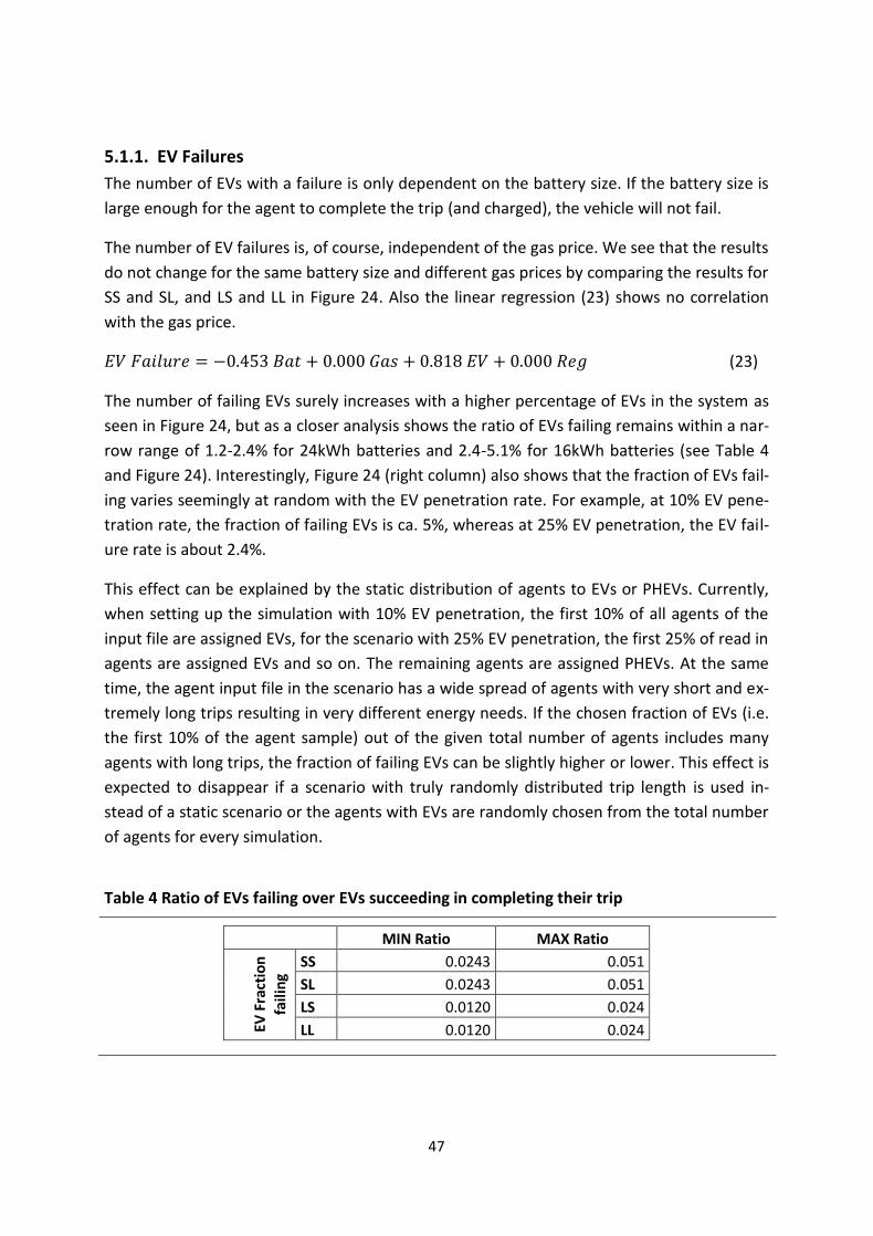
5.1.1. EV Failures
The number of EVs with a failure is only dependent on the battery size. If the battery size is
large enough for the agent to complete the trip (and charged), the vehicle will not fail.
The number of EV failures is, of course, independent of the gas price. We see that the results
do not change for the same battery size and different gas prices by comparing the results for
SS and SL, and LS and LL in Figure 24. Also the linear regression (23) shows no correlation
with the gas price.
(23)
The number of failing EVs surely increases with a higher percentage of EVs in the system as
seen in Figure 24, but as a closer analysis shows the ratio of EVs failing remains within a nar-
row range of 1.2-2.4% for 24kWh batteries and 2.4-5.1% for 16kWh batteries (see Table 4
and Figure 24). Interestingly, Figure 24 (right column) also shows that the fraction of EVs fail-
ing varies seemingly at random with the EV penetration rate. For example, at 10% EV pene-
tration rate, the fraction of failing EVs is ca. 5%, whereas at 25% EV penetration, the EV fail-
ure rate is about 2.4%.
This effect can be explained by the static distribution of agents to EVs or PHEVs. Currently,
when setting up the simulation with 10% EV penetration, the first 10% of all agents of the
input file are assigned EVs, for the scenario with 25% EV penetration, the first 25% of read in
agents are assigned EVs and so on. The remaining agents are assigned PHEVs. At the same
time, the agent input file in the scenario has a wide spread of agents with very short and ex-
tremely long trips resulting in very different energy needs. If the chosen fraction of EVs (i.e.
the first 10% of the agent sample) out of the given total number of agents includes many
agents with long trips, the fraction of failing EVs can be slightly higher or lower. This effect is
expected to disappear if a scenario with truly randomly distributed trip length is used in-
stead of a static scenario or the agents with EVs are randomly chosen from the total number
of agents for every simulation.
Table 4 Ratio of EVs failing over EVs succeeding in completing their trip
MIN Ratio MAX Ratio
EV F
ract
ion
faili
ng
SS 0.0243 0.051
SL 0.0243 0.051
LS 0.0120 0.024
LL 0.0120 0.024
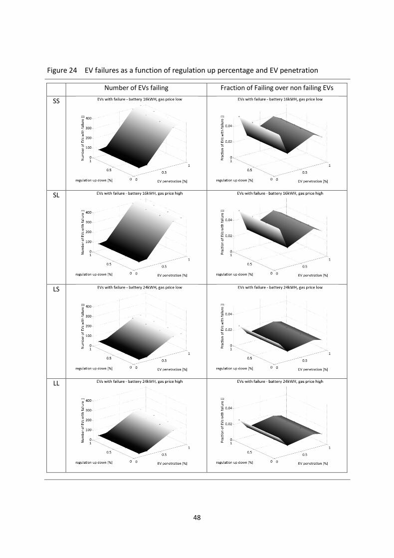
48
Figure 24 EV failures as a function of regulation up percentage and EV penetration
Number of EVs failing Fraction of Failing over non failing EVs
SS
SL
LS
LL
49
5.1.2. Charging duration
As Figure 25 and the corresponding linear regressions (23) and (24) show, the charging time for EVs and PHEVs is mainly dependent on the battery size and is independent of the gas price. If the battery size is large, a large energy reserve can be used to travel greater distances, but also requires more time to be recharged. As table 5 shows, the difference in the average charging time for small and large batteries is about two hours. Table 5 also shows, that EVs seem to charge slightly longer than PHEVs. This is probably the case, because whenever PHEVs have the choice to go below the SOC of 10% or to use their combustion engine, EVs will be forced to continue charging. It can also be seen, that the gas price has no influence on the charging duration of PHEVs. It would be interesting to see, if this result changes for an even lower gas price. In the used US price scenario it is only more expensive to charge electricity than to use gas at the very end of the day, where no more charging is required. Thus the charging behavior is not visibly al-tered. Of course, the charging duration is independent of the percentage of agents providing regu-lation up and down since it is calculated within the decentralized smart charging algorithm before the V2G simulation. Figure 25 also shows that the charging duration for EVs increases minimally for low EV pene-trations. This is probably a random effect related to the relatively large ratio of EVs failing at this particular EV level (compare to 5.1.1.) because of the static distribution of agents to ve-hicle types. (23) (24)
Table 5 Minimum and Maximum average charging times across all simulations
all EV PHEV
Charging Time [s] MIN 16430.36 16419.49 16352.50
MAX 23364.87 23952.21 23429.97
Charging Time [h] MIN 4.56 4.56 4.54
MAX 6.49 6.65 6.51
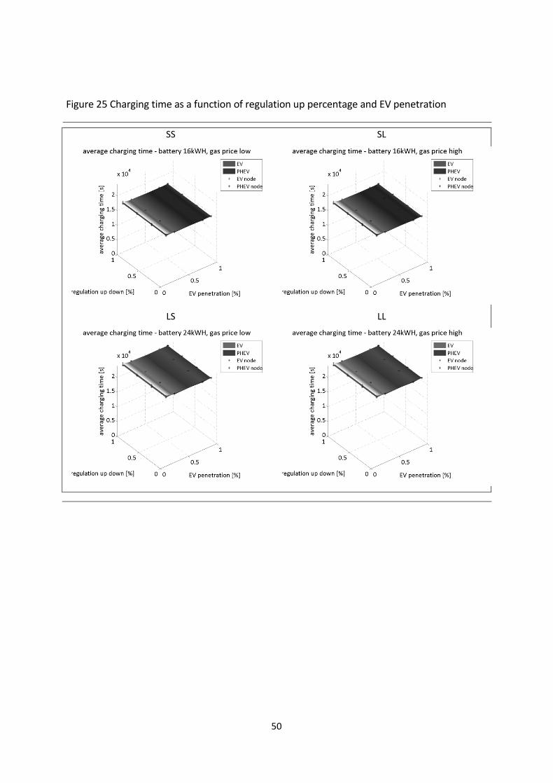
50
Figure 25 Charging time as a function of regulation up percentage and EV penetration
SS
SL
LS
LL
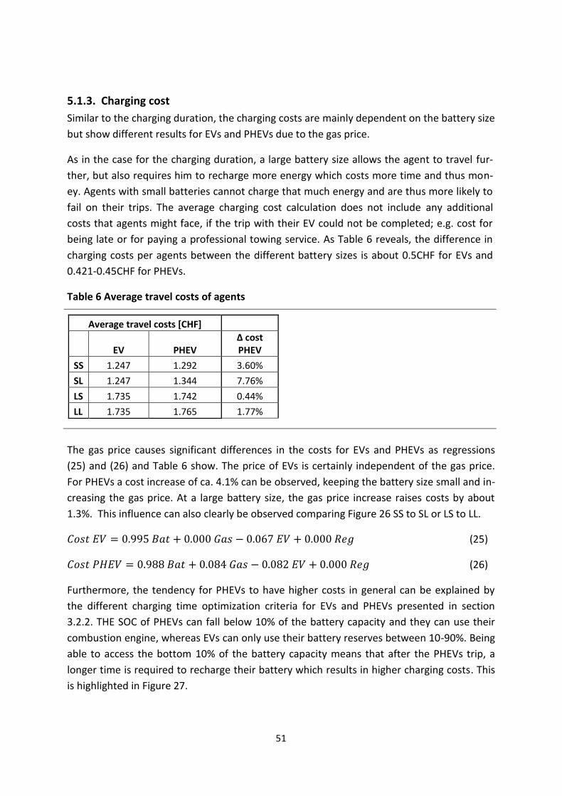
51
5.1.3. Charging cost
Similar to the charging duration, the charging costs are mainly dependent on the battery size
but show different results for EVs and PHEVs due to the gas price.
As in the case for the charging duration, a large battery size allows the agent to travel fur-
ther, but also requires him to recharge more energy which costs more time and thus mon-
ey. Agents with small batteries cannot charge that much energy and are thus more likely to
fail on their trips. The average charging cost calculation does not include any additional
costs that agents might face, if the trip with their EV could not be completed; e.g. cost for
being late or for paying a professional towing service. As Table 6 reveals, the difference in
charging costs per agents between the different battery sizes is about 0.5CHF for EVs and
0.421-0.45CHF for PHEVs.
Table 6 Average travel costs of agents
Average travel costs [CHF]
EV PHEV Δ cost PHEV
SS 1.247 1.292 3.60%
SL 1.247 1.344 7.76%
LS 1.735 1.742 0.44%
LL 1.735 1.765 1.77%
The gas price causes significant differences in the costs for EVs and PHEVs as regressions
(25) and (26) and Table 6 show. The price of EVs is certainly independent of the gas price.
For PHEVs a cost increase of ca. 4.1% can be observed, keeping the battery size small and in-
creasing the gas price. At a large battery size, the gas price increase raises costs by about
1.3%. This influence can also clearly be observed comparing Figure 26 SS to SL or LS to LL.
(25)
(26)
Furthermore, the tendency for PHEVs to have higher costs in general can be explained by
the different charging time optimization criteria for EVs and PHEVs presented in section
3.2.2. THE SOC of PHEVs can fall below 10% of the battery capacity and they can use their
combustion engine, whereas EVs can only use their battery reserves between 10-90%. Being
able to access the bottom 10% of the battery capacity means that after the PHEVs trip, a
longer time is required to recharge their battery which results in higher charging costs. This
is highlighted in Figure 27.

52
Of course, there is also a certain bias in the system. In cases where restricted EVs fail, PHEVs
will be able to complete their longer trips. Longer trips are bound to be more expensive. This
raises the average cost for PHEVs.
If one looks at the exact shape of the cost as a function of the EV penetration, one discovers small variations. Again this phenomenon can be explained by the distribution of trip lengths in the sample of agents as discussed in 5.1.1. For example, the costs for EVs at the penetra-tion rate of 10% are highest, which correlates to a high ratio of EVs failing. Every vehicle with long trips which is bound to fail maximizes its charging length, consequently these agents charge at any price which results in high charging costs.
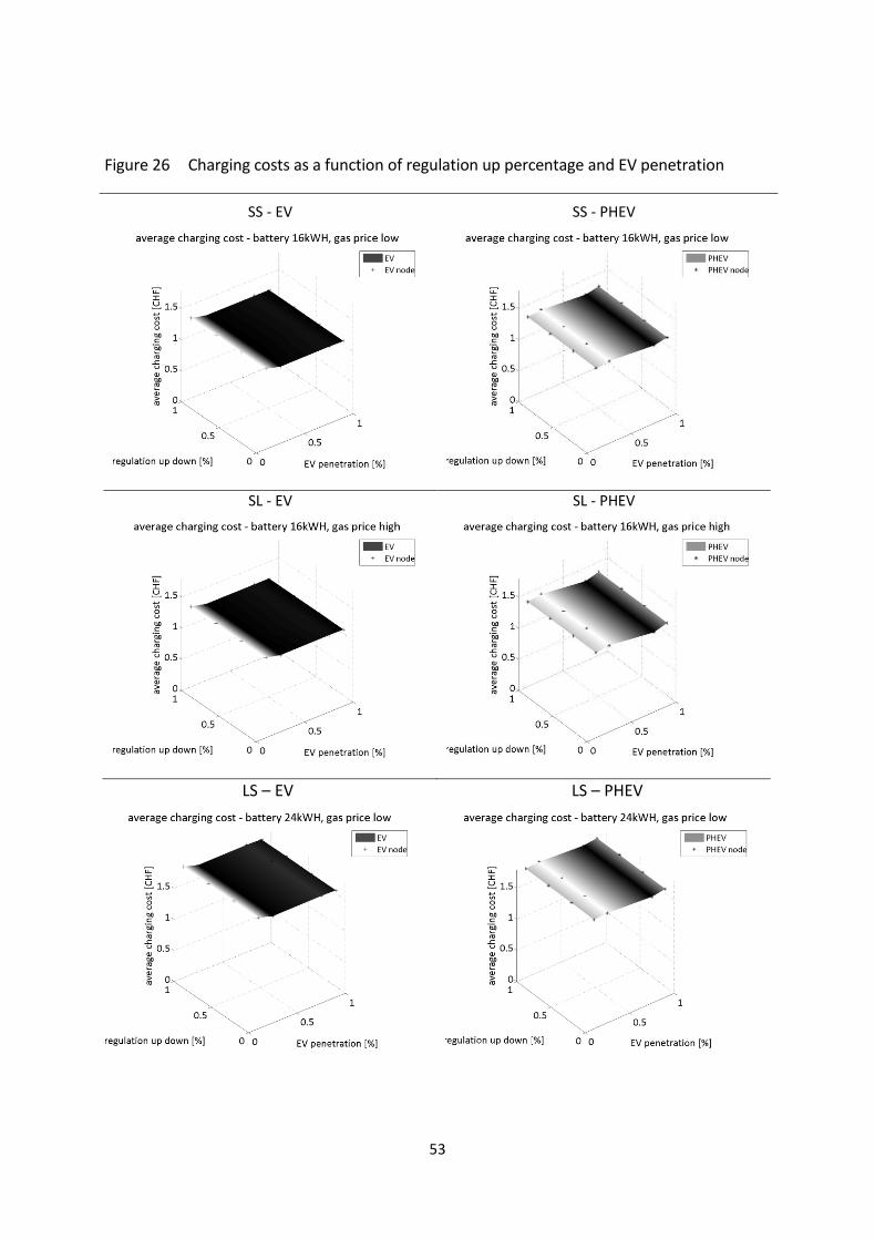
53
Figure 26 Charging costs as a function of regulation up percentage and EV penetration
SS - EV
SS - PHEV
SL - EV
SL - PHEV
LS – EV
LS – PHEV
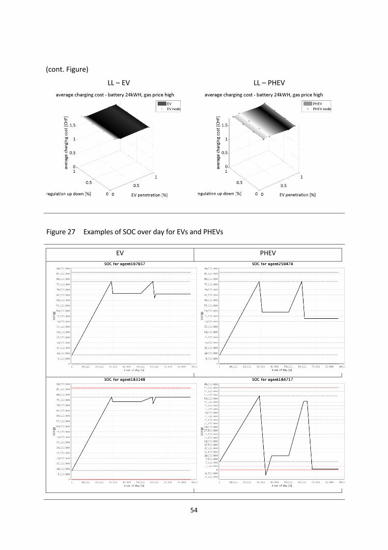
54
(cont. Figure)
LL – EV
LL – PHEV
Figure 27 Examples of SOC over day for EVs and PHEVs
EV PHEV
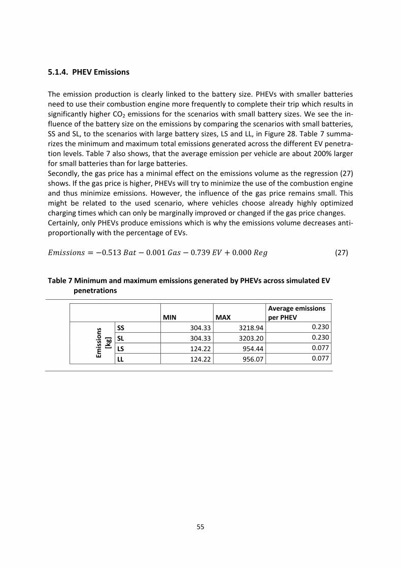
55
5.1.4. PHEV Emissions
The emission production is clearly linked to the battery size. PHEVs with smaller batteries need to use their combustion engine more frequently to complete their trip which results in significantly higher CO2 emissions for the scenarios with small battery sizes. We see the in-fluence of the battery size on the emissions by comparing the scenarios with small batteries, SS and SL, to the scenarios with large battery sizes, LS and LL, in Figure 28. Table 7 summa-rizes the minimum and maximum total emissions generated across the different EV penetra-tion levels. Table 7 also shows, that the average emission per vehicle are about 200% larger for small batteries than for large batteries. Secondly, the gas price has a minimal effect on the emissions volume as the regression (27) shows. If the gas price is higher, PHEVs will try to minimize the use of the combustion engine and thus minimize emissions. However, the influence of the gas price remains small. This might be related to the used scenario, where vehicles choose already highly optimized charging times which can only be marginally improved or changed if the gas price changes. Certainly, only PHEVs produce emissions which is why the emissions volume decreases anti-proportionally with the percentage of EVs. (27)
Table 7 Minimum and maximum emissions generated by PHEVs across simulated EV
penetrations
MIN MAX
Average emissions per PHEV
Emis
sio
ns
[kg]
SS 304.33 3218.94 0.230
SL 304.33 3203.20 0.230
LS 124.22 954.44 0.077
LL 124.22 956.07 0.077
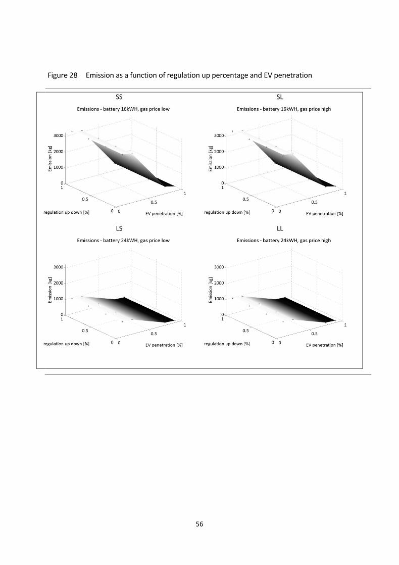
56
Figure 28 Emission as a function of regulation up percentage and EV penetration
SS
SL
LS
LL
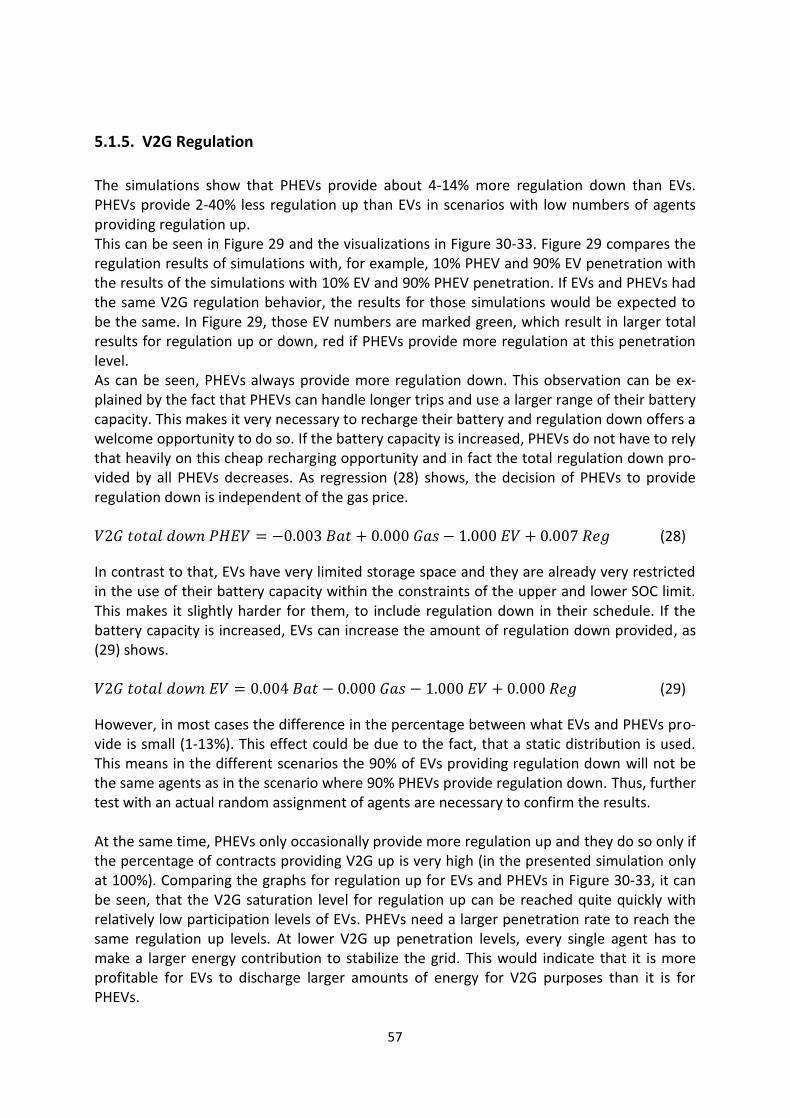
57
5.1.5. V2G Regulation
The simulations show that PHEVs provide about 4-14% more regulation down than EVs. PHEVs provide 2-40% less regulation up than EVs in scenarios with low numbers of agents providing regulation up. This can be seen in Figure 29 and the visualizations in Figure 30-33. Figure 29 compares the regulation results of simulations with, for example, 10% PHEV and 90% EV penetration with the results of the simulations with 10% EV and 90% PHEV penetration. If EVs and PHEVs had the same V2G regulation behavior, the results for those simulations would be expected to be the same. In Figure 29, those EV numbers are marked green, which result in larger total results for regulation up or down, red if PHEVs provide more regulation at this penetration level. As can be seen, PHEVs always provide more regulation down. This observation can be ex-plained by the fact that PHEVs can handle longer trips and use a larger range of their battery capacity. This makes it very necessary to recharge their battery and regulation down offers a welcome opportunity to do so. If the battery capacity is increased, PHEVs do not have to rely that heavily on this cheap recharging opportunity and in fact the total regulation down pro-vided by all PHEVs decreases. As regression (28) shows, the decision of PHEVs to provide regulation down is independent of the gas price. (28)
In contrast to that, EVs have very limited storage space and they are already very restricted in the use of their battery capacity within the constraints of the upper and lower SOC limit. This makes it slightly harder for them, to include regulation down in their schedule. If the battery capacity is increased, EVs can increase the amount of regulation down provided, as (29) shows. (29)
However, in most cases the difference in the percentage between what EVs and PHEVs pro-vide is small (1-13%). This effect could be due to the fact, that a static distribution is used. This means in the different scenarios the 90% of EVs providing regulation down will not be the same agents as in the scenario where 90% PHEVs provide regulation down. Thus, further test with an actual random assignment of agents are necessary to confirm the results. At the same time, PHEVs only occasionally provide more regulation up and they do so only if the percentage of contracts providing V2G up is very high (in the presented simulation only at 100%). Comparing the graphs for regulation up for EVs and PHEVs in Figure 30-33, it can be seen, that the V2G saturation level for regulation up can be reached quite quickly with relatively low participation levels of EVs. PHEVs need a larger penetration rate to reach the same regulation up levels. At lower V2G up penetration levels, every single agent has to make a larger energy contribution to stabilize the grid. This would indicate that it is more profitable for EVs to discharge larger amounts of energy for V2G purposes than it is for PHEVs.

58
Again, it might also be the case that the static assignment of agents to vehicles and to con-tract types might be the reason for slight distortions. As can be seen, the agents have similar regulation up behavior at a 100% regulation up participation rate at which the effect of the static distribution obviously does not influence the results.
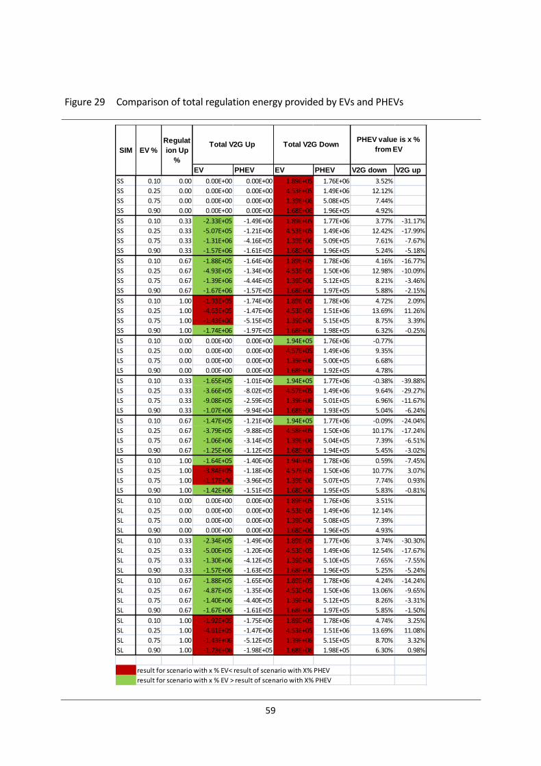
59
Figure 29 Comparison of total regulation energy provided by EVs and PHEVs
EV PHEV EV PHEV V2G down V2G up
SS 0.10 0.00 0.00E+00 0.00E+00 1.89E+05 1.76E+06 3.52%
SS 0.25 0.00 0.00E+00 0.00E+00 4.53E+05 1.49E+06 12.12%
SS 0.75 0.00 0.00E+00 0.00E+00 1.39E+06 5.08E+05 7.44%
SS 0.90 0.00 0.00E+00 0.00E+00 1.68E+06 1.96E+05 4.92%
SS 0.10 0.33 -2.33E+05 -1.49E+06 1.89E+05 1.77E+06 3.77% -31.17%
SS 0.25 0.33 -5.07E+05 -1.21E+06 4.53E+05 1.49E+06 12.42% -17.99%
SS 0.75 0.33 -1.31E+06 -4.16E+05 1.39E+06 5.09E+05 7.61% -7.67%
SS 0.90 0.33 -1.57E+06 -1.61E+05 1.68E+06 1.96E+05 5.24% -5.18%
SS 0.10 0.67 -1.88E+05 -1.64E+06 1.89E+05 1.78E+06 4.16% -16.77%
SS 0.25 0.67 -4.93E+05 -1.34E+06 4.53E+05 1.50E+06 12.98% -10.09%
SS 0.75 0.67 -1.39E+06 -4.44E+05 1.39E+06 5.12E+05 8.21% -3.46%
SS 0.90 0.67 -1.67E+06 -1.57E+05 1.68E+06 1.97E+05 5.88% -2.15%
SS 0.10 1.00 -1.93E+05 -1.74E+06 1.89E+05 1.78E+06 4.72% 2.09%
SS 0.25 1.00 -4.63E+05 -1.47E+06 4.53E+05 1.51E+06 13.69% 11.26%
SS 0.75 1.00 -1.43E+06 -5.15E+05 1.39E+06 5.15E+05 8.75% 3.39%
SS 0.90 1.00 -1.74E+06 -1.97E+05 1.68E+06 1.98E+05 6.32% -0.25%
LS 0.10 0.00 0.00E+00 0.00E+00 1.94E+05 1.76E+06 -0.77%
LS 0.25 0.00 0.00E+00 0.00E+00 4.57E+05 1.49E+06 9.35%
LS 0.75 0.00 0.00E+00 0.00E+00 1.39E+06 5.00E+05 6.68%
LS 0.90 0.00 0.00E+00 0.00E+00 1.68E+06 1.92E+05 4.78%
LS 0.10 0.33 -1.65E+05 -1.01E+06 1.94E+05 1.77E+06 -0.38% -39.88%
LS 0.25 0.33 -3.66E+05 -8.02E+05 4.57E+05 1.49E+06 9.64% -29.27%
LS 0.75 0.33 -9.08E+05 -2.59E+05 1.39E+06 5.01E+05 6.96% -11.67%
LS 0.90 0.33 -1.07E+06 -9.94E+04 1.68E+06 1.93E+05 5.04% -6.24%
LS 0.10 0.67 -1.47E+05 -1.21E+06 1.94E+05 1.77E+06 -0.09% -24.04%
LS 0.25 0.67 -3.79E+05 -9.88E+05 4.58E+05 1.50E+06 10.17% -17.24%
LS 0.75 0.67 -1.06E+06 -3.14E+05 1.39E+06 5.04E+05 7.39% -6.51%
LS 0.90 0.67 -1.25E+06 -1.12E+05 1.68E+06 1.94E+05 5.45% -3.02%
LS 0.10 1.00 -1.64E+05 -1.40E+06 1.94E+05 1.78E+06 0.59% -7.45%
LS 0.25 1.00 -3.84E+05 -1.18E+06 4.57E+05 1.50E+06 10.77% 3.07%
LS 0.75 1.00 -1.17E+06 -3.96E+05 1.39E+06 5.07E+05 7.74% 0.93%
LS 0.90 1.00 -1.42E+06 -1.51E+05 1.68E+06 1.95E+05 5.83% -0.81%
SL 0.10 0.00 0.00E+00 0.00E+00 1.89E+05 1.76E+06 3.51%
SL 0.25 0.00 0.00E+00 0.00E+00 4.53E+05 1.49E+06 12.14%
SL 0.75 0.00 0.00E+00 0.00E+00 1.39E+06 5.08E+05 7.39%
SL 0.90 0.00 0.00E+00 0.00E+00 1.68E+06 1.96E+05 4.93%
SL 0.10 0.33 -2.34E+05 -1.49E+06 1.89E+05 1.77E+06 3.74% -30.30%
SL 0.25 0.33 -5.00E+05 -1.20E+06 4.53E+05 1.49E+06 12.54% -17.67%
SL 0.75 0.33 -1.30E+06 -4.12E+05 1.39E+06 5.10E+05 7.65% -7.55%
SL 0.90 0.33 -1.57E+06 -1.63E+05 1.68E+06 1.96E+05 5.25% -5.24%
SL 0.10 0.67 -1.88E+05 -1.65E+06 1.89E+05 1.78E+06 4.24% -14.24%
SL 0.25 0.67 -4.87E+05 -1.35E+06 4.53E+05 1.50E+06 13.06% -9.65%
SL 0.75 0.67 -1.40E+06 -4.40E+05 1.39E+06 5.12E+05 8.26% -3.31%
SL 0.90 0.67 -1.67E+06 -1.61E+05 1.68E+06 1.97E+05 5.85% -1.50%
SL 0.10 1.00 -1.92E+05 -1.75E+06 1.89E+05 1.78E+06 4.74% 3.25%
SL 0.25 1.00 -4.61E+05 -1.47E+06 4.53E+05 1.51E+06 13.69% 11.08%
SL 0.75 1.00 -1.43E+06 -5.12E+05 1.39E+06 5.15E+05 8.70% 3.32%
SL 0.90 1.00 -1.73E+06 -1.98E+05 1.68E+06 1.98E+05 6.30% 0.98%
result for scenario with x % EV< result of scenario with X% PHEV
result for scenario with x % EV > result of scenario with X% PHEV
PHEV value is x %
from EVEV %
Regulat
ion Up
%
SIMTotal V2G Down Total V2G Up
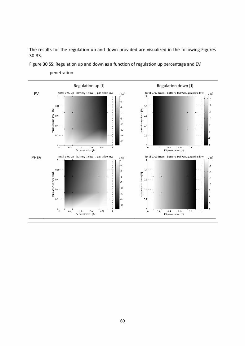
60
The results for the regulation up and down provided are visualized in the following Figures 30-33.
Figure 30 SS: Regulation up and down as a function of regulation up percentage and EV
penetration
Regulation up [J] Regulation down [J]
EV
PHEV
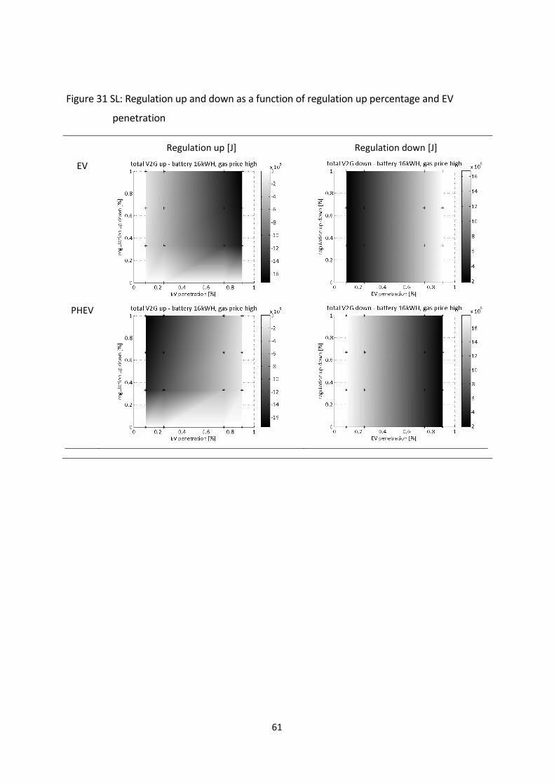
61
Figure 31 SL: Regulation up and down as a function of regulation up percentage and EV
penetration
Regulation up [J] Regulation down [J]
EV
PHEV
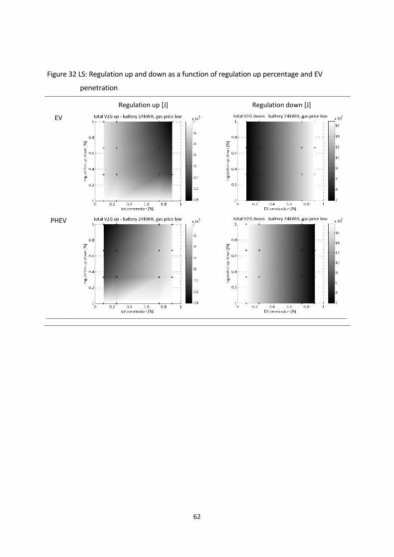
62
Figure 32 LS: Regulation up and down as a function of regulation up percentage and EV
penetration
Regulation up [J] Regulation down [J]
EV
PHEV

63
Figure 33 LL: Regulation up and down as a function of regulation up percentage and EV
penetration
Regulation up [J] Regulation down [J]
EV
PHEV
64
5.1.6. V2G Revenue
From the presented regulation up and down behavior, the revenue profiles can be derived for EVs and PHEVs (Figure 35-38). Revenue in the simulation is defined as the sum of (i) di-rect earnings from compensation for providing regulation and (ii) the indirect savings ob-tained from being able to improve one’s schedule by rescheduling meaning the difference between the costs of keeping the current schedule and rescheduling the day. It can be seen, that the total direct compensation increases for EVs and PHEVs with higher penetrations of V2G regulation-up contracts to a total sum of maximally around 0.05 CHF for all EVs and PHEVs, the indirect savings vary tremendously from simulation to simulation and agent to agent. As the second row of graphs in Figures 35-38 shows, the total direct compensation is very similar for EVs and PHEVs approaching a total sum of 0.05 CHF per day across all agents for small batteries and 0.04 CHF for large batteries. In parallel to the rapid increase in V2G regu-lation up for EVs at lower EV penetration levels (as discussed in 5.1.5), also the compensa-tion increases more rapidly for EVs. In contrast to the direct revenue, the indirect savings are highly dependent on the agent’s plans and the chosen charging times and may range up to a total sum of 200CHF across all agents or more. The total indirect savings are on average much higher for PHEVs which can be explained by the rescheduling costs. Because PHEVs have so much planning flexibility thanks to their battery and combustion engine, rescheduling costs are generally lower. This changes drastically, if the gas price is increased which reduces the flexibility of PHEVs; in-creasing the gas price results in a drop of the maximum total indirect savings from a sum of over 200 CHF in scenario SS (Figure 35 bottom right) to only about 60CHF in scenario SL (Fig-ure 36 bottom right). Similarly, an increase in the battery size also increases the scheduling flexibility, which leads to an increase in the indirect savings for EVs (from ca. 0.3 CHF (Figure 35 bottom left) to over 2 CHF (Figure 37 bottom left)) and PHEVS from ca. 200CHF (Figure 35 bottom right) in SS to almost 250 CHF in LS (Figure 37 bottom right). Comparing the revenues from direct compensation and indirect savings for EVs and PHEVs for one example simulation (see Figure 34), it becomes clear, that although EVs do get on average larger direct compensations, PHEVs can leverage much greater savings by the nu-merous rescheduling opportunities thanks to their low rescheduling costs. Thus, overall, PHEVs benefit more from participating in V2G. Nevertheless, the total revenues from V2G are mostly negligible for single private vehicles. Thus, it might be more interesting for large scale vehicle fleets to pool the capacities of all their vehicles together for V2G purposes. Al-ternatively, larger compensations and attractive contracts could incentivize vehicles to par-ticipate in such a V2G model.
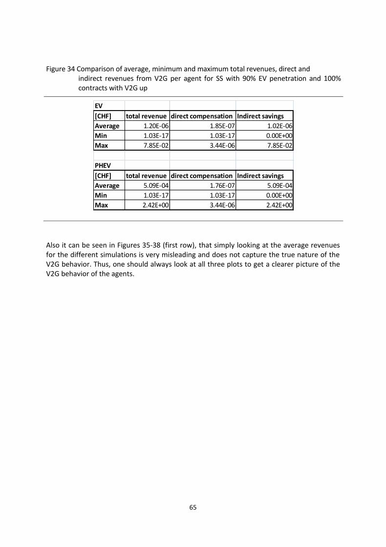
65
Figure 34 Comparison of average, minimum and maximum total revenues, direct and indirect revenues from V2G per agent for SS with 90% EV penetration and 100% contracts with V2G up
Also it can be seen in Figures 35-38 (first row), that simply looking at the average revenues for the different simulations is very misleading and does not capture the true nature of the V2G behavior. Thus, one should always look at all three plots to get a clearer picture of the V2G behavior of the agents.
EV
[CHF] total revenue direct compensation Indirect savings
Average 1.20E-06 1.85E-07 1.02E-06
Min 1.03E-17 1.03E-17 0.00E+00
Max 7.85E-02 3.44E-06 7.85E-02
PHEV
[CHF] total revenue direct compensation Indirect savings
Average 5.09E-04 1.76E-07 5.09E-04
Min 1.03E-17 1.03E-17 0.00E+00
Max 2.42E+00 3.44E-06 2.42E+00
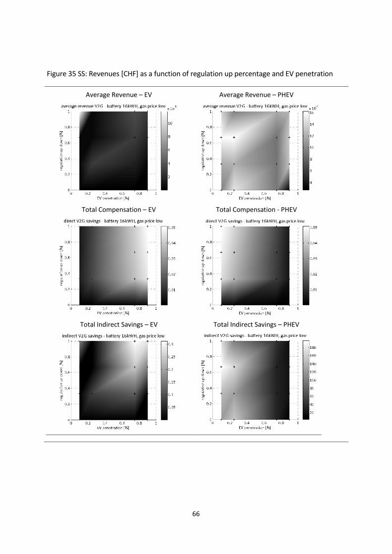
66
Figure 35 SS: Revenues [CHF] as a function of regulation up percentage and EV penetration
Average Revenue – EV Average Revenue – PHEV
Total Compensation – EV Total Compensation - PHEV
Total Indirect Savings – EV Total Indirect Savings – PHEV
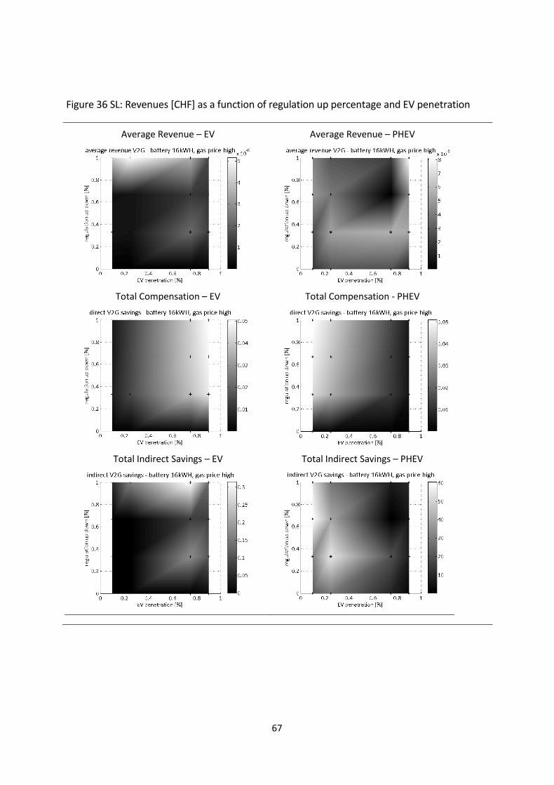
67
Figure 36 SL: Revenues [CHF] as a function of regulation up percentage and EV penetration
Average Revenue – EV Average Revenue – PHEV
Total Compensation – EV Total Compensation - PHEV
Total Indirect Savings – EV Total Indirect Savings – PHEV
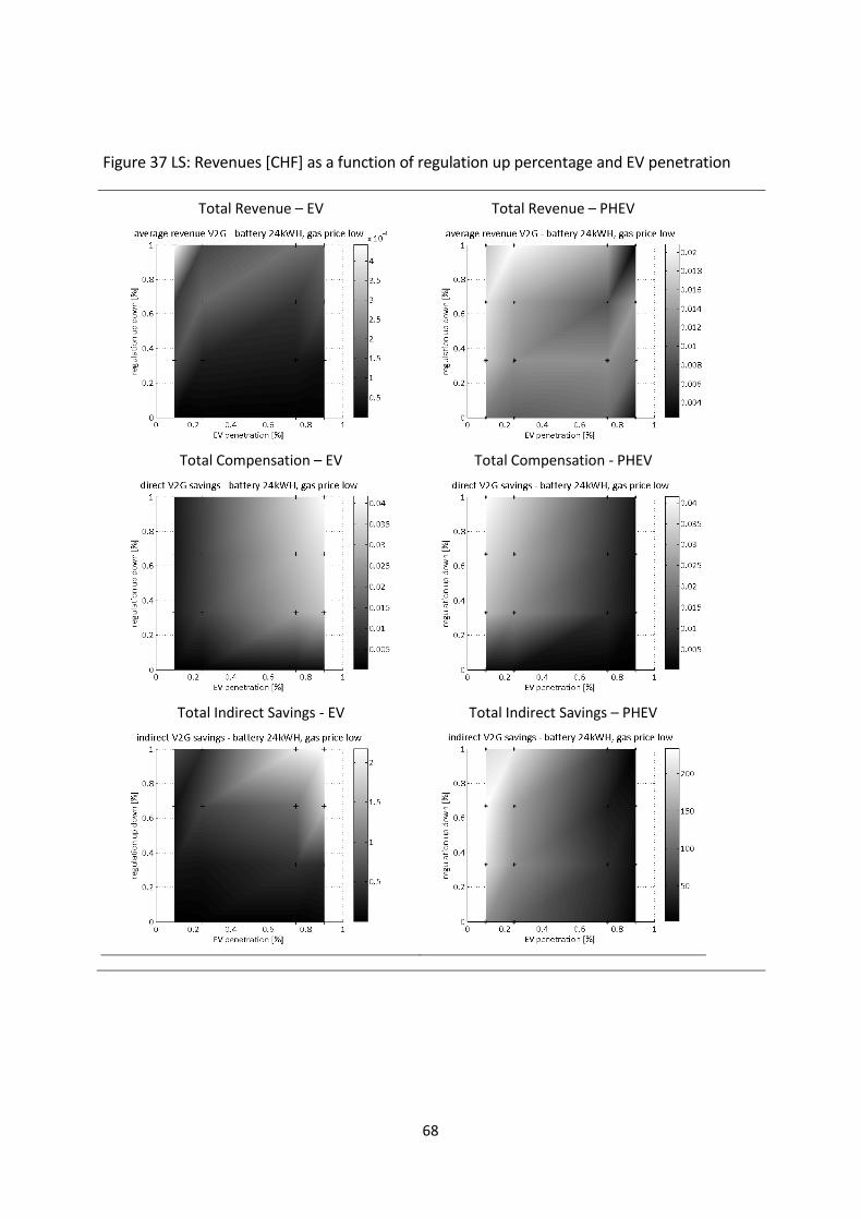
68
Figure 37 LS: Revenues [CHF] as a function of regulation up percentage and EV penetration
Total Revenue – EV Total Revenue – PHEV
Total Compensation – EV Total Compensation - PHEV
Total Indirect Savings - EV Total Indirect Savings – PHEV
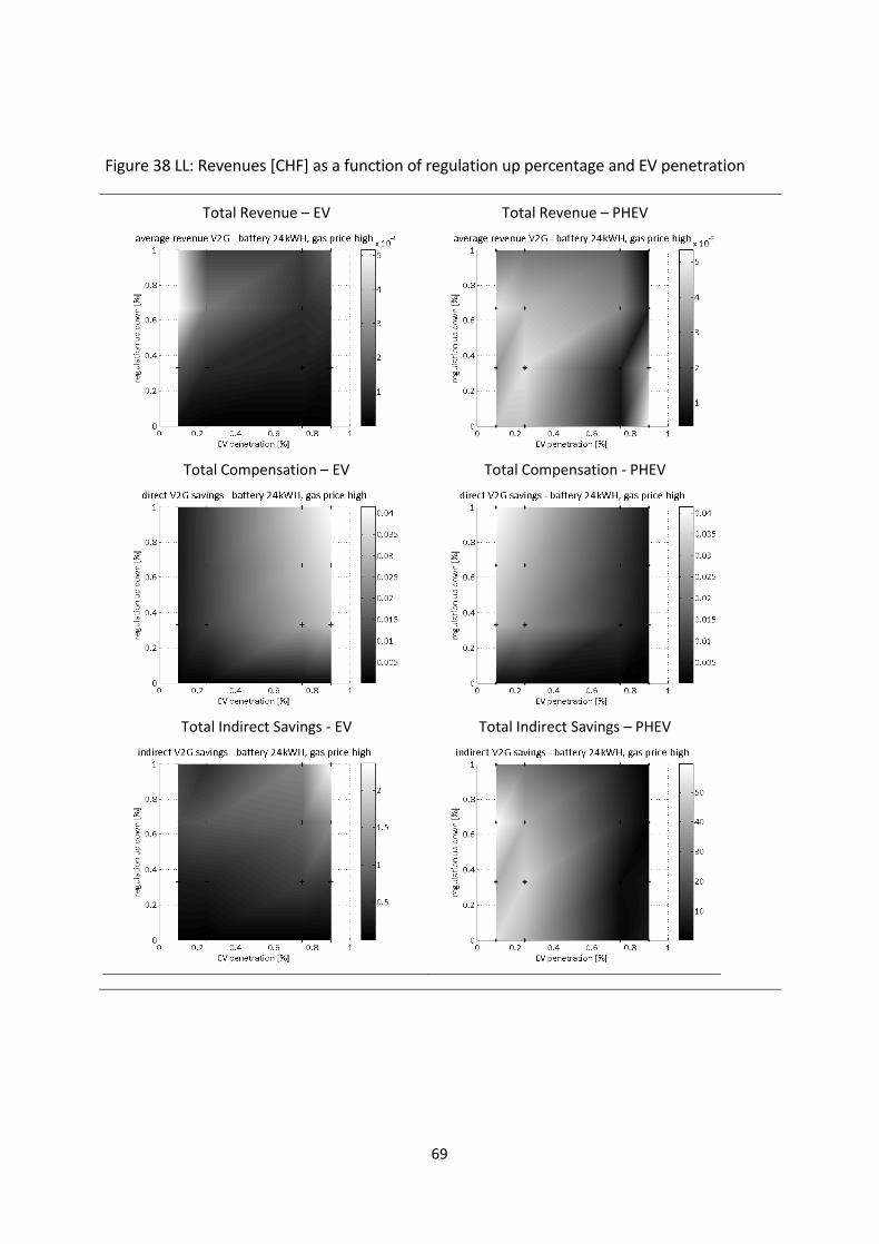
69
Figure 38 LL: Revenues [CHF] as a function of regulation up percentage and EV penetration
Total Revenue – EV Total Revenue – PHEV
Total Compensation – EV Total Compensation - PHEV
Total Indirect Savings - EV Total Indirect Savings – PHEV
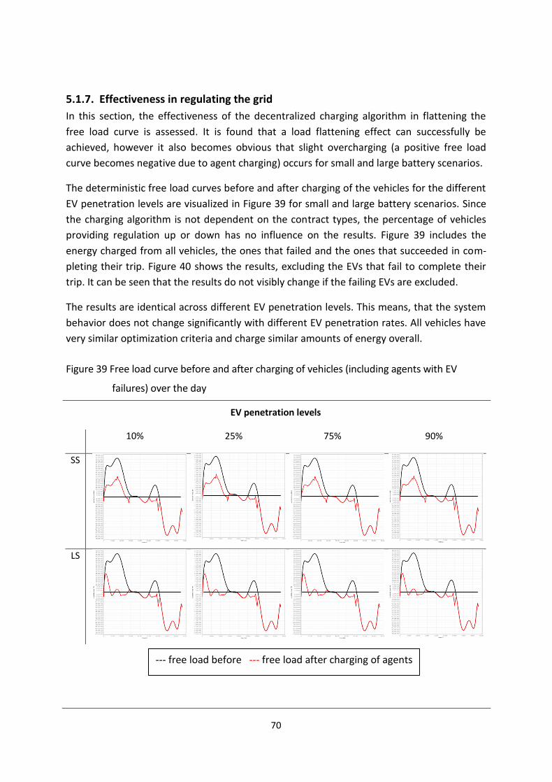
70
5.1.7. Effectiveness in regulating the grid
In this section, the effectiveness of the decentralized charging algorithm in flattening the
free load curve is assessed. It is found that a load flattening effect can successfully be
achieved, however it also becomes obvious that slight overcharging (a positive free load
curve becomes negative due to agent charging) occurs for small and large battery scenarios.
The deterministic free load curves before and after charging of the vehicles for the different
EV penetration levels are visualized in Figure 39 for small and large battery scenarios. Since
the charging algorithm is not dependent on the contract types, the percentage of vehicles
providing regulation up or down has no influence on the results. Figure 39 includes the
energy charged from all vehicles, the ones that failed and the ones that succeeded in com-
pleting their trip. Figure 40 shows the results, excluding the EVs that fail to complete their
trip. It can be seen that the results do not visibly change if the failing EVs are excluded.
The results are identical across different EV penetration levels. This means, that the system
behavior does not change significantly with different EV penetration rates. All vehicles have
very similar optimization criteria and charge similar amounts of energy overall.
Figure 39 Free load curve before and after charging of vehicles (including agents with EV
failures) over the day
EV penetration levels
10% 25% 75% 90%
SS
LS
--- free load before --- free load after charging of agents
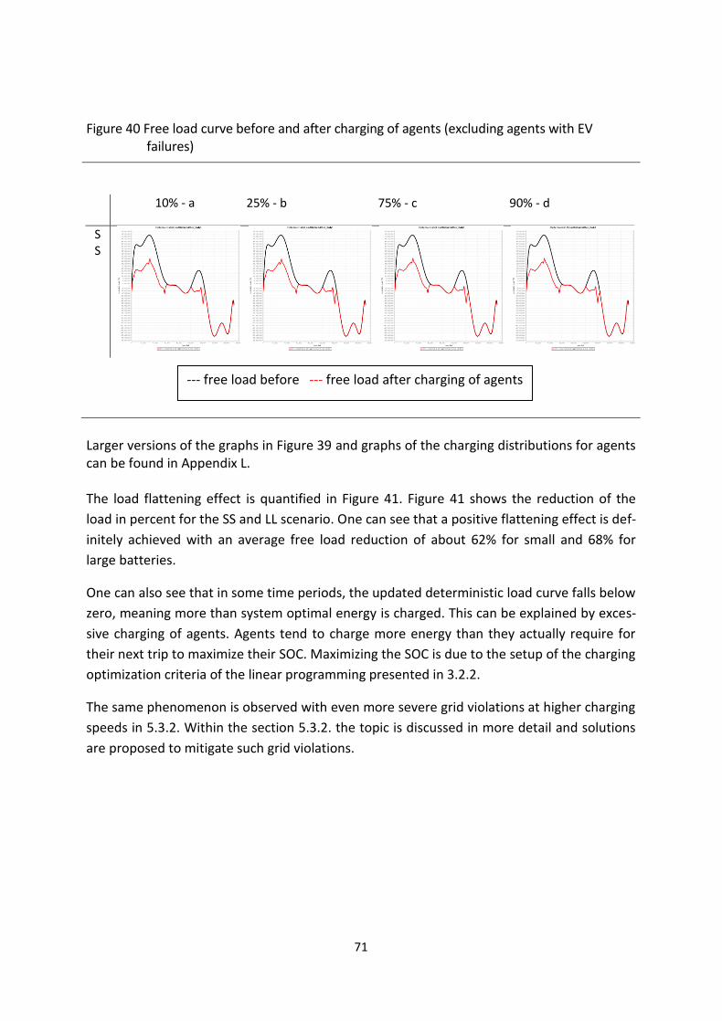
71
Figure 40 Free load curve before and after charging of agents (excluding agents with EV failures)
10% - a 25% - b 75% - c 90% - d
SS
Larger versions of the graphs in Figure 39 and graphs of the charging distributions for agents can be found in Appendix L. The load flattening effect is quantified in Figure 41. Figure 41 shows the reduction of the
load in percent for the SS and LL scenario. One can see that a positive flattening effect is def-
initely achieved with an average free load reduction of about 62% for small and 68% for
large batteries.
One can also see that in some time periods, the updated deterministic load curve falls below
zero, meaning more than system optimal energy is charged. This can be explained by exces-
sive charging of agents. Agents tend to charge more energy than they actually require for
their next trip to maximize their SOC. Maximizing the SOC is due to the setup of the charging
optimization criteria of the linear programming presented in 3.2.2.
The same phenomenon is observed with even more severe grid violations at higher charging
speeds in 5.3.2. Within the section 5.3.2. the topic is discussed in more detail and solutions
are proposed to mitigate such grid violations.
--- free load before --- free load after charging of agents
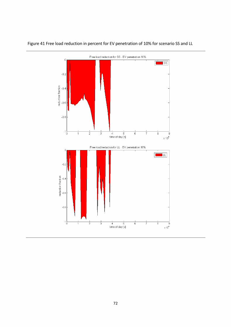
72
Figure 41 Free load reduction in percent for EV penetration of 10% for scenario SS and LL
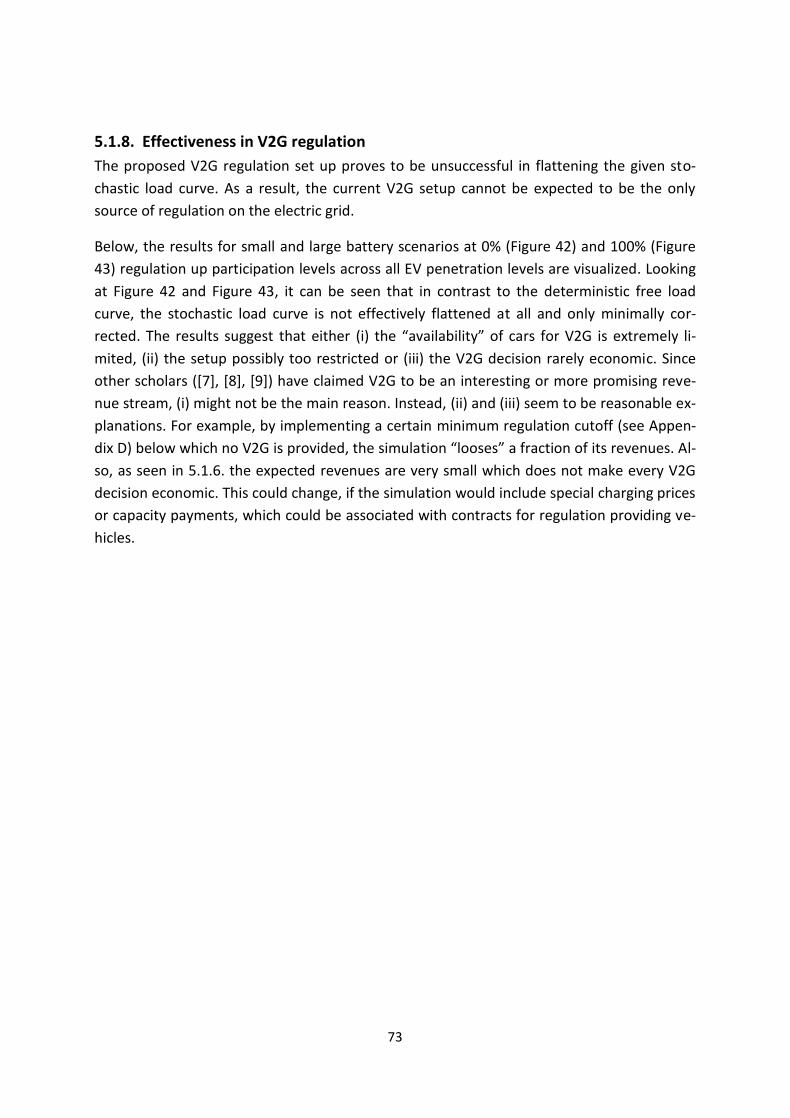
73
5.1.8. Effectiveness in V2G regulation
The proposed V2G regulation set up proves to be unsuccessful in flattening the given sto-
chastic load curve. As a result, the current V2G setup cannot be expected to be the only
source of regulation on the electric grid.
Below, the results for small and large battery scenarios at 0% (Figure 42) and 100% (Figure
43) regulation up participation levels across all EV penetration levels are visualized. Looking
at Figure 42 and Figure 43, it can be seen that in contrast to the deterministic free load
curve, the stochastic load curve is not effectively flattened at all and only minimally cor-
rected. The results suggest that either (i) the “availability” of cars for V2G is extremely li-
mited, (ii) the setup possibly too restricted or (iii) the V2G decision rarely economic. Since
other scholars ([7], [8], [9]) have claimed V2G to be an interesting or more promising reve-
nue stream, (i) might not be the main reason. Instead, (ii) and (iii) seem to be reasonable ex-
planations. For example, by implementing a certain minimum regulation cutoff (see Appen-
dix D) below which no V2G is provided, the simulation “looses” a fraction of its revenues. Al-
so, as seen in 5.1.6. the expected revenues are very small which does not make every V2G
decision economic. This could change, if the simulation would include special charging prices
or capacity payments, which could be associated with contracts for regulation providing ve-
hicles.
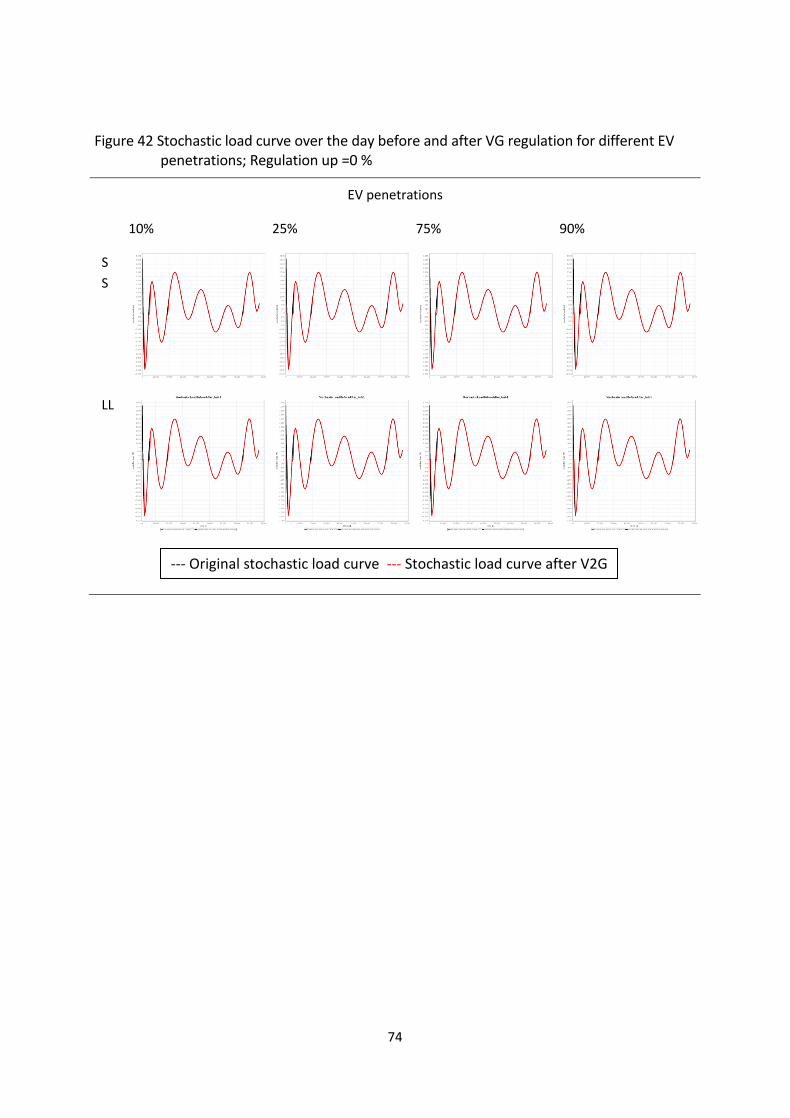
74
Figure 42 Stochastic load curve over the day before and after VG regulation for different EV penetrations; Regulation up =0 %
EV penetrations
10% 25% 75% 90%
S
S
LL
--- Original stochastic load curve --- Stochastic load curve after V2G
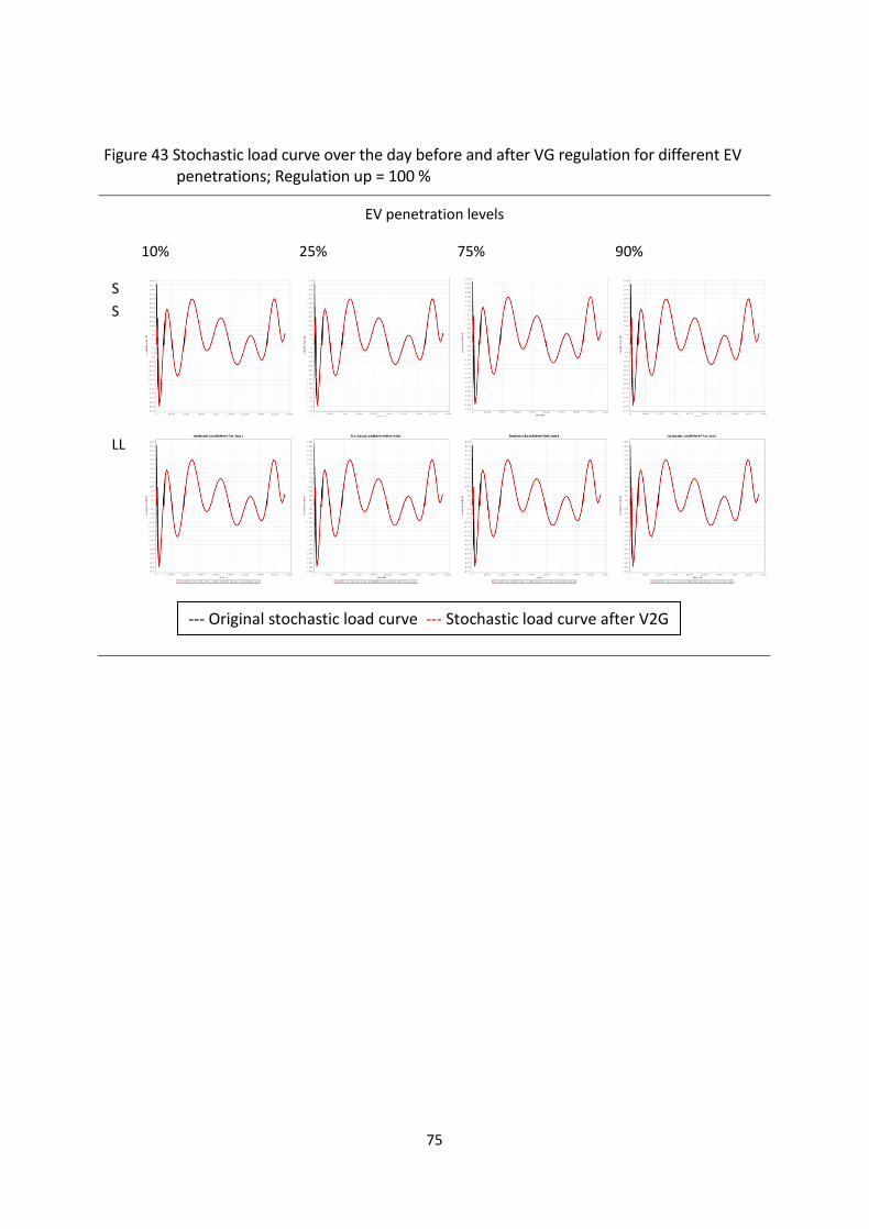
75
Figure 43 Stochastic load curve over the day before and after VG regulation for different EV penetrations; Regulation up = 100 %
EV penetration levels
10% 25% 75% 90%
S
S
LL
--- Original stochastic load curve --- Stochastic load curve after V2G
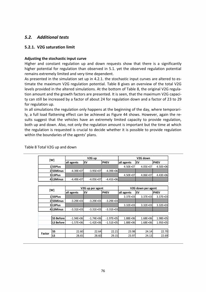
76
5.2. Additional tests
5.2.1. V2G saturation limit
Adjusting the stochastic input curve Higher and constant regulation up and down requests show that there is a significantly higher potential for regulation than observed in 5.1. yet the observed regulation potential remains extremely limited and very time dependent. As presented in the simulation set up in 4.2.1. the stochastic input curves are altered to es-timate the maximum V2G regulation potential. Table 8 gives an overview of the total V2G levels provided in the altered simulations. At the bottom of Table 8, the original V2G regula-tion amount and the growth factors are presented. It is seen, that the maximum V2G capaci-ty can still be increased by a factor of about 24 for regulation down and a factor of 23 to 29 for regulation up. In all simulations the regulation only happens at the beginning of the day, where temporari-ly, a full load flattening effect can be achieved as Figure 44 shows. However, again the re-sults suggest that the vehicles have an extremely limited capacity to provide regulation, both up and down. Also, not only the regulation amount is important but the time at which the regulation is requested is crucial to decide whether it is possible to provide regulation within the boundaries of the agents’ plans.
Table 8 Total V2G up and down
all agents EV PHEV all agents EV PHEV
1 SSPlus 4.50E+07 4.05E+07 4.50E+06
2 SSMinus -4.39E+07 -3.95E+07 -4.39E+06
3 LSPlus 4.50E+07 4.06E+07 4.43E+06
4 LSMinus -4.49E+07 -4.05E+07 -4.41E+06
all agents EV PHEV all agents EV PHEV
1 SSPlus 3.37E+03 3.37E+03 3.37E+03
2 SSMinus -3.29E+03 -3.29E+03 -3.29E+03
3 LSPlus 3.32E+03 3.32E+03 3.32E+03
4 LSMinus -3.31E+03 -3.31E+03 -3.31E+03
SS Before -1.94E+06 -1.74E+06 -1.97E+05 1.88E+06 1.68E+06 1.98E+05
LS Before -1.57E+06 -1.42E+06 -1.51E+05 1.88E+06 1.68E+06 1.95E+05
SS 22.60 22.64 22.21 23.98 24.14 22.70
LS 28.65 28.60 29.15 23.97 24.13 22.69Factor
V2G up V2G down[W]
[W]V2G up per agent V2G down per agent
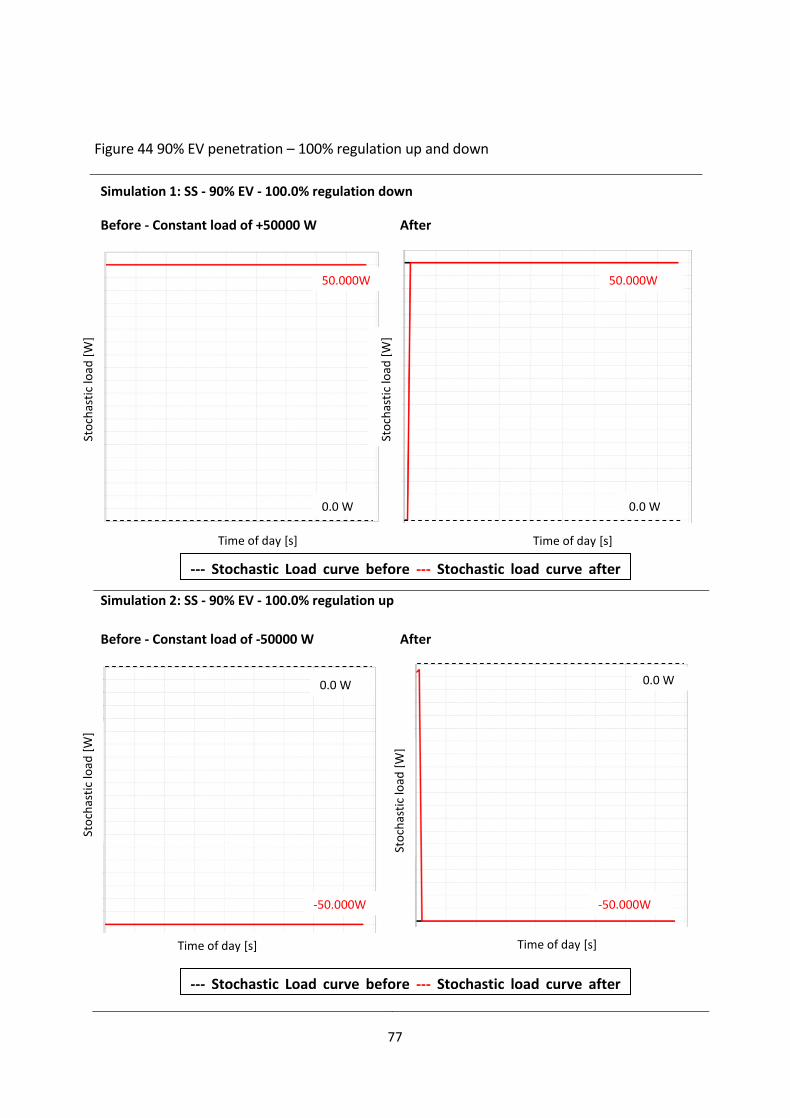
77
Figure 44 90% EV penetration – 100% regulation up and down
Simulation 1: SS - 90% EV - 100.0% regulation down
Before - Constant load of +50000 W
After
Simulation 2: SS - 90% EV - 100.0% regulation up
Before - Constant load of -50000 W
After
Time of day [s] Time of day [s]
Time of day [s] Time of day [s]
Sto
chas
tic
load
[W
]
Sto
chas
tic
load
[W
]
--- Stochastic Load curve before --- Stochastic load curve after V2G
Sto
chas
tic
load
[W
]
50.000W
-50.000W
Sto
chas
tic
load
[W
]
0.0 W 0.0 W
-50.000W
50.000W
0.0 W 0.0 W
--- Stochastic Load curve before --- Stochastic load curve after V2G
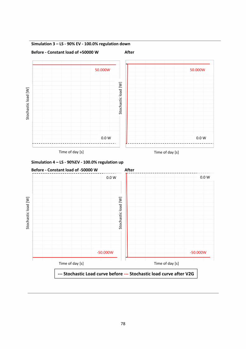
78
Simulation 3 – LS - 90% EV - 100.0% regulation down
Before - Constant load of +50000 W After
Simulation 4 – LS - 90%EV - 100.0% regulation up
Before - Constant load of -50000 W After
--- Stochastic Load curve before --- Stochastic load curve after V2G
Time of day [s] Time of day [s]
Sto
chas
tic
load
[W
]
Sto
chas
tic
load
[W
]
0.0 W 0.0 W
0.0 W 0.0 W
-50.000W -50.000W
50.000W 50.000W
Sto
chas
tic
load
[W
] St
och
asti
c lo
ad [
W]
Sto
chas
tic
load
[W
]
Time of day [s] Time of day [s]
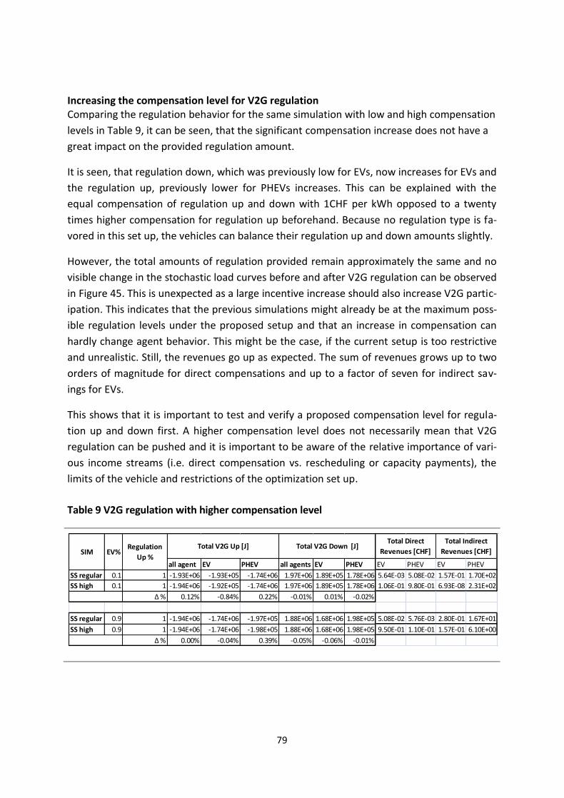
79
Increasing the compensation level for V2G regulation Comparing the regulation behavior for the same simulation with low and high compensation
levels in Table 9, it can be seen, that the significant compensation increase does not have a
great impact on the provided regulation amount.
It is seen, that regulation down, which was previously low for EVs, now increases for EVs and
the regulation up, previously lower for PHEVs increases. This can be explained with the
equal compensation of regulation up and down with 1CHF per kWh opposed to a twenty
times higher compensation for regulation up beforehand. Because no regulation type is fa-
vored in this set up, the vehicles can balance their regulation up and down amounts slightly.
However, the total amounts of regulation provided remain approximately the same and no
visible change in the stochastic load curves before and after V2G regulation can be observed
in Figure 45. This is unexpected as a large incentive increase should also increase V2G partic-
ipation. This indicates that the previous simulations might already be at the maximum poss-
ible regulation levels under the proposed setup and that an increase in compensation can
hardly change agent behavior. This might be the case, if the current setup is too restrictive
and unrealistic. Still, the revenues go up as expected. The sum of revenues grows up to two
orders of magnitude for direct compensations and up to a factor of seven for indirect sav-
ings for EVs.
This shows that it is important to test and verify a proposed compensation level for regula-
tion up and down first. A higher compensation level does not necessarily mean that V2G
regulation can be pushed and it is important to be aware of the relative importance of vari-
ous income streams (i.e. direct compensation vs. rescheduling or capacity payments), the
limits of the vehicle and restrictions of the optimization set up.
Table 9 V2G regulation with higher compensation level
all agent EV PHEV all agents EV PHEV EV PHEV EV PHEV
SS regular 0.1 1 -1.93E+06 -1.93E+05 -1.74E+06 1.97E+06 1.89E+05 1.78E+06 5.64E-03 5.08E-02 1.57E-01 1.70E+02
SS high 0.1 1 -1.94E+06 -1.92E+05 -1.74E+06 1.97E+06 1.89E+05 1.78E+06 1.06E-01 9.80E-01 6.93E-08 2.31E+02
Δ % 0.12% -0.84% 0.22% -0.01% 0.01% -0.02%
SS regular 0.9 1 -1.94E+06 -1.74E+06 -1.97E+05 1.88E+06 1.68E+06 1.98E+05 5.08E-02 5.76E-03 2.80E-01 1.67E+01
SS high 0.9 1 -1.94E+06 -1.74E+06 -1.98E+05 1.88E+06 1.68E+06 1.98E+05 9.50E-01 1.10E-01 1.57E-01 6.10E+00
Δ % 0.00% -0.04% 0.39% -0.05% -0.06% -0.01%
Total Direct
Revenues [CHF]
Total Indirect
Revenues [CHF]EV%Regulation
Up %SIM
Total V2G Down [J]Total V2G Up [J]

80
Figure 45 Stochastic load curves before and after V2G for scenario with low and high compensation
Regular compensation - SSP High Compensation SSP
5.2.2. Charging speed
Implementing a higher charging speed leads to significantly higher electric grid violations in the afternoon and more energy over all being charged from the grid as seen in Figure 46. Increasing the charging speed does also not necessarily mean that less vehicles will fail to complete their trip, since failure in the given simulation setup is mainly connected to the battery size and not to a limit in charging opportunities. Overcharging phenomenon Important lessons about the current set up and its implications for the charging behavior of agents can be deducted from the observed “overcharging” of agents, meaning charging more than the agent actually needs to complete his next trips safely. Agents generally want to maximize their SOC and thus the agents take advantage of the fast charging opportunity in optimal charging times. An example of such an overcharging agent is given in Figure 47. The agent charges far more than he actually needs and recharges his bat-tery fully after the second driving interval. He thus puts extra strains on the grid even though he is charging in an optimal time period.
--- stochastic load curve before --- stochastic load curve after V2G
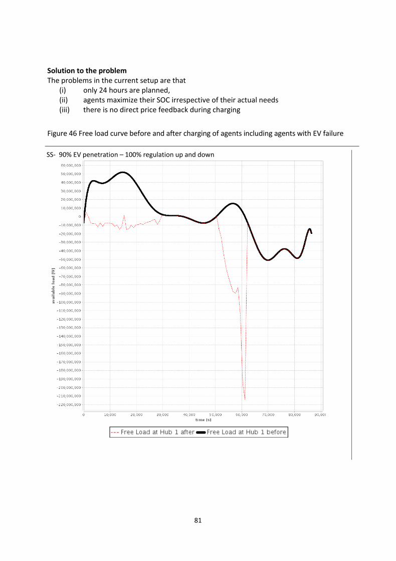
81
Solution to the problem The problems in the current setup are that
(i) only 24 hours are planned, (ii) agents maximize their SOC irrespective of their actual needs (iii) there is no direct price feedback during charging
Figure 46 Free load curve before and after charging of agents including agents with EV failure
SS- 90% EV penetration – 100% regulation up and down
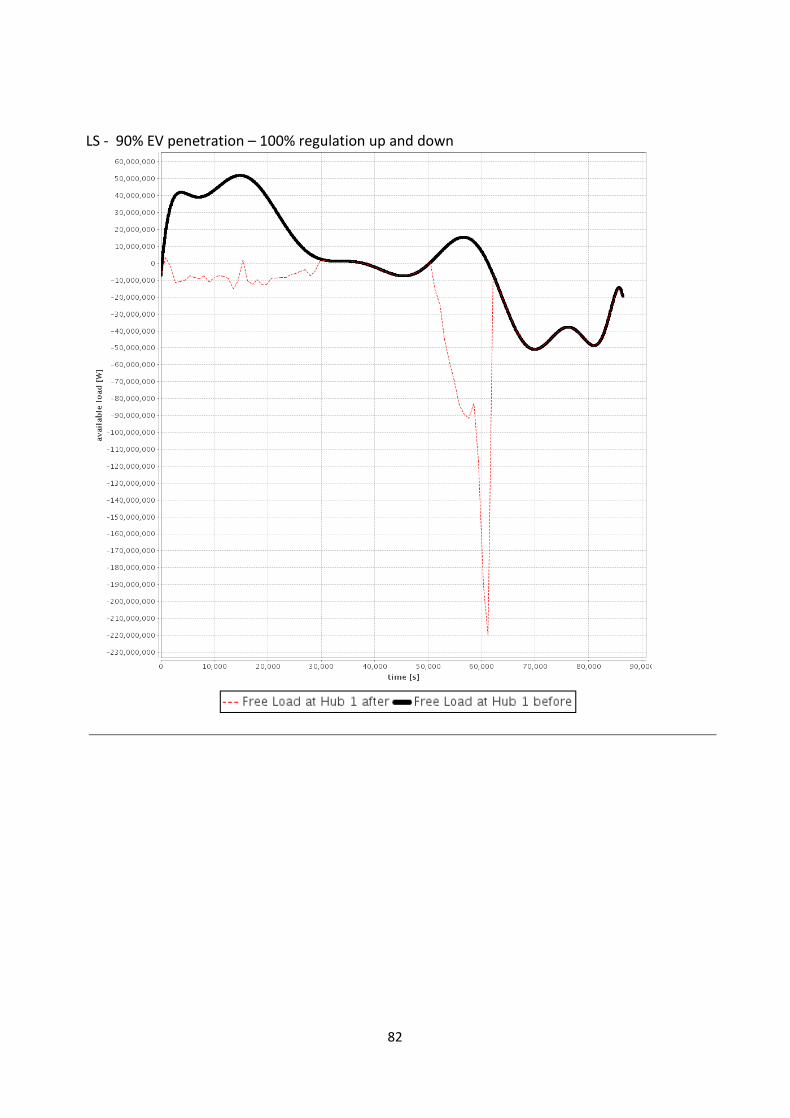
82
LS - 90% EV penetration – 100% regulation up and down
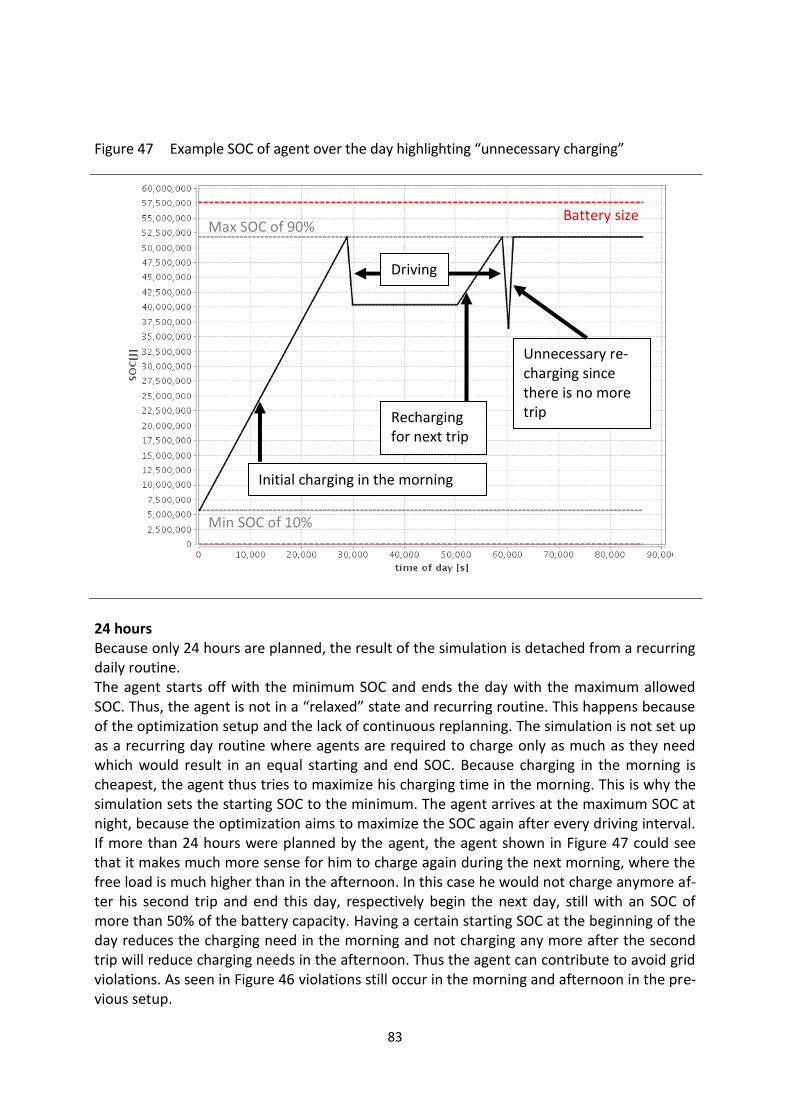
83
Figure 47 Example SOC of agent over the day highlighting “unnecessary charging”
24 hours Because only 24 hours are planned, the result of the simulation is detached from a recurring daily routine. The agent starts off with the minimum SOC and ends the day with the maximum allowed SOC. Thus, the agent is not in a “relaxed” state and recurring routine. This happens because of the optimization setup and the lack of continuous replanning. The simulation is not set up as a recurring day routine where agents are required to charge only as much as they need which would result in an equal starting and end SOC. Because charging in the morning is cheapest, the agent thus tries to maximize his charging time in the morning. This is why the simulation sets the starting SOC to the minimum. The agent arrives at the maximum SOC at night, because the optimization aims to maximize the SOC again after every driving interval. If more than 24 hours were planned by the agent, the agent shown in Figure 47 could see that it makes much more sense for him to charge again during the next morning, where the free load is much higher than in the afternoon. In this case he would not charge anymore af-ter his second trip and end this day, respectively begin the next day, still with an SOC of more than 50% of the battery capacity. Having a certain starting SOC at the beginning of the day reduces the charging need in the morning and not charging any more after the second trip will reduce charging needs in the afternoon. Thus the agent can contribute to avoid grid violations. As seen in Figure 46 violations still occur in the morning and afternoon in the pre-vious setup.
Initial charging in the morning
Driving
Recharging for next trip
Unnecessary re-charging since there is no more trip
Battery size Max SOC of 90%
Min SOC of 10%

84
The impact of having continuous planning is shown by simulating the same recurring day and artificially fixing the starting SOC at 50% of the battery capacity (the charge left from the previous day). This is an attempt to “simulate” a recurring day routine. A 24 hour optimiza-tion has previously been done already for centralized smart charging in [4]. In Figure 48 it can be seen that grid violations in the first few hours of the day can be miti-gated completely. Again the extreme grid violations in the afternoon remain because no ac-tual replanning is implemented and the behavior of the agents in the second half of the day remains the same. The associated diagram of the state of charge over the day for an exam-ple agent is presented in Figure 49.
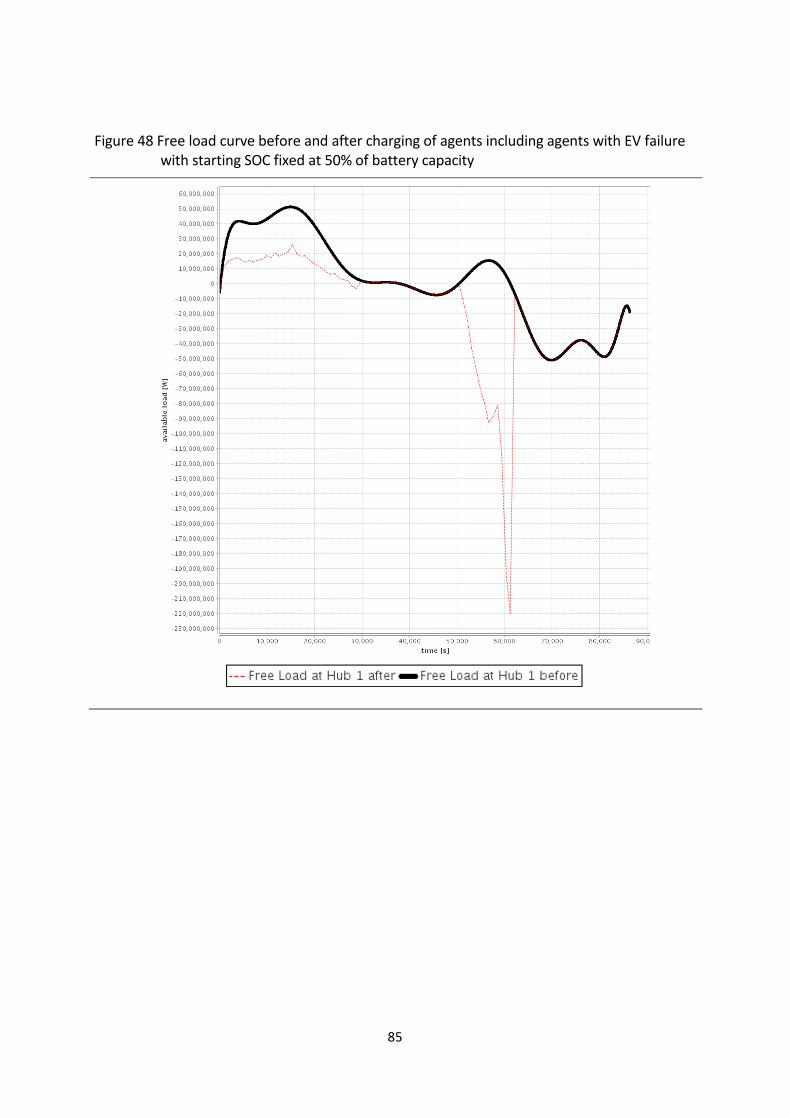
85
Figure 48 Free load curve before and after charging of agents including agents with EV failure with starting SOC fixed at 50% of battery capacity
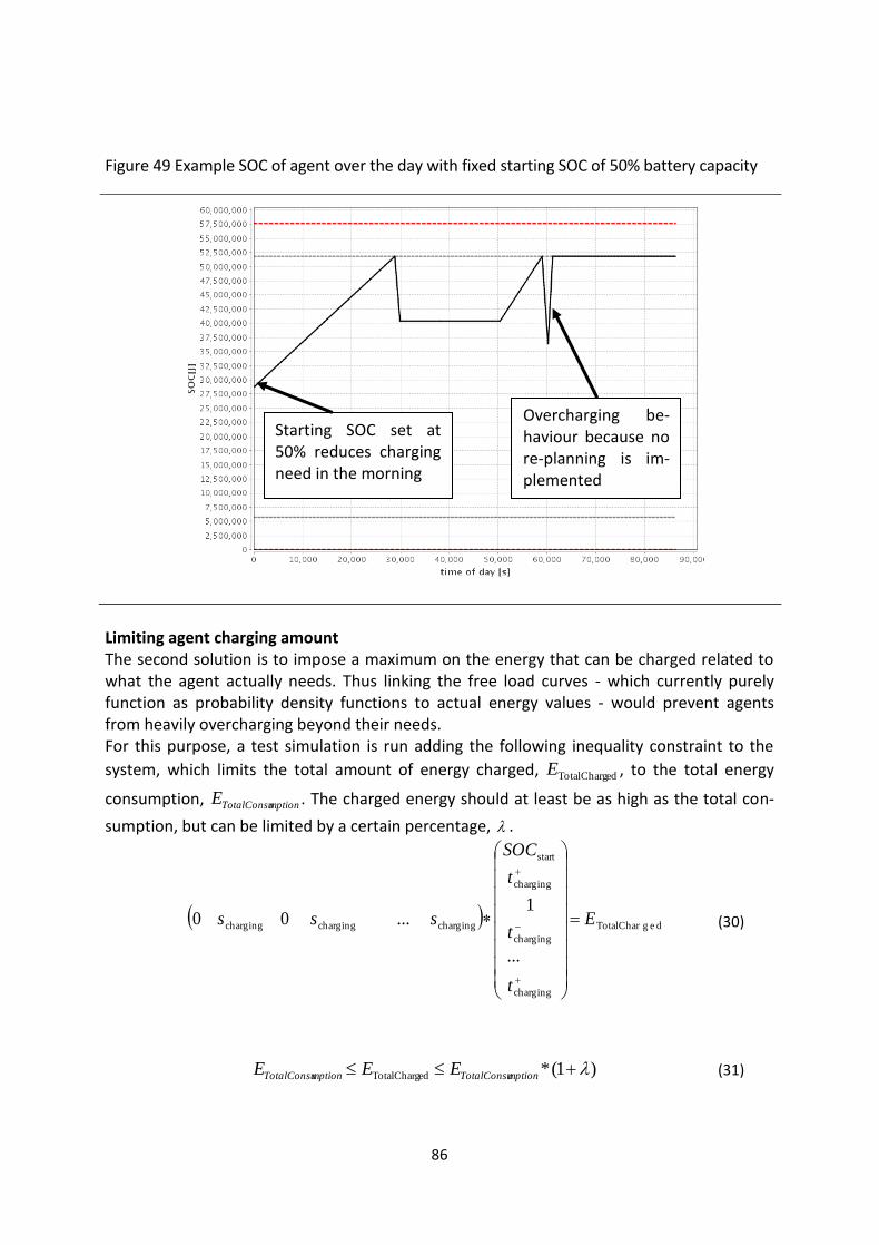
86
Figure 49 Example SOC of agent over the day with fixed starting SOC of 50% battery capacity
Limiting agent charging amount The second solution is to impose a maximum on the energy that can be charged related to what the agent actually needs. Thus linking the free load curves - which currently purely function as probability density functions to actual energy values - would prevent agents from heavily overcharging beyond their needs. For this purpose, a test simulation is run adding the following inequality constraint to the
system, which limits the total amount of energy charged, edTotalChargE , to the total energy
consumption, mptionTotalConsuE . The charged energy should at least be as high as the total con-
sumption, but can be limited by a certain percentage, .
d e g TotalChar
charging
charging
charging
start
chargingchargingcharging
...
1 ... 0 0 E
t
t
t
SOC
sss
(30)
)1(*edTotalCharg mptionTotalConsumptionTotalConsu EEE (31)
Starting SOC set at 50% reduces charging need in the morning
Overcharging be-haviour because no re-planning is im-plemented
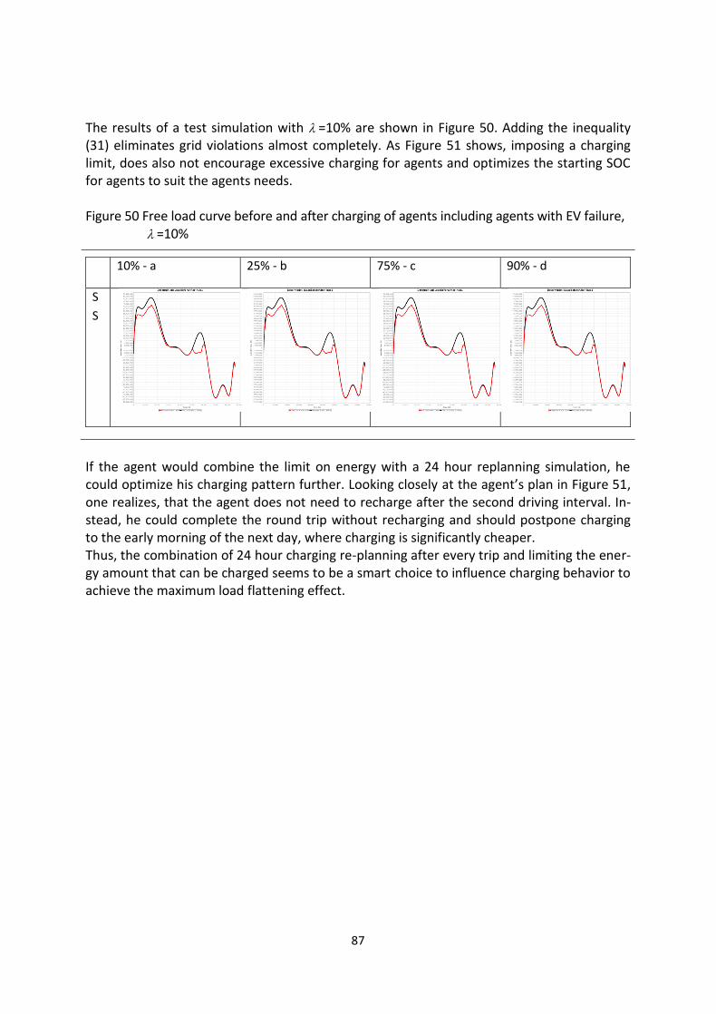
87
The results of a test simulation with =10% are shown in Figure 50. Adding the inequality (31) eliminates grid violations almost completely. As Figure 51 shows, imposing a charging limit, does also not encourage excessive charging for agents and optimizes the starting SOC for agents to suit the agents needs. Figure 50 Free load curve before and after charging of agents including agents with EV failure,
=10%
10% - a 25% - b 75% - c 90% - d
S
S
If the agent would combine the limit on energy with a 24 hour replanning simulation, he could optimize his charging pattern further. Looking closely at the agent’s plan in Figure 51, one realizes, that the agent does not need to recharge after the second driving interval. In-stead, he could complete the round trip without recharging and should postpone charging to the early morning of the next day, where charging is significantly cheaper. Thus, the combination of 24 hour charging re-planning after every trip and limiting the ener-gy amount that can be charged seems to be a smart choice to influence charging behavior to achieve the maximum load flattening effect.
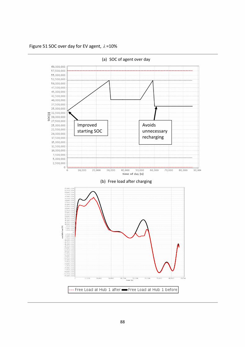
88
Figure 51 SOC over day for EV agent, =10%
(a) SOC of agent over day
(b) Free load after charging
Improved starting SOC
Avoids unnecessary recharging

89
Feedback Feedback on violations can be given by adjusting the free load curves to influence and alter charging behavior. The goal is to suppress charging in the afternoon and only encourage charging in the morn-ing. This is why it is attempted to change the free load curve to only have positive values in the morning and to suppress charging in the afternoon by making the free load curve nega-tive for the rest of the day. However, results of changing the free load curve presented in Figure 52 clearly show, that this does not solve the problem. The charging amounts are still completely detached from the actually available free load. Instead, probably not only the load curve but also the related price curve should be altered. The issue with such a solution is the need for significantly more communication infrastruc-ture to synchronize the parameters for free load curves as well as prices in the cars. This is less favorable because this infrastructure heavy set up is again closer to a centralized ap-proach.
Figure 52 Free load curve with positive values only in the morning has no positive influence on the charging behavior (including agents with EV failure, EV penetration of 90%)
90
6. Discussion
6.1. Decentralized Smart Charging Algorithm
The decentralized smart charging algorithm presented here clearly proves to be a powerful tool to optimize charging behavior. The algorithm clearly flattens the given free load curve and is thus superior to dumb charging or time of use pricing strategies which can result in severe grid violations as shown by [4]. Especially if the improvement strategies discussed in 5.2.2 are integrated – (i) a continuous charging time replanning after every driving interval and (ii) a certain limit on how much more energy can be charged than needed - grid violations can be completely mitigated. Furthermore, the solution is found in one step and no iterations are needed to find the sys-tem optimal solution. In contrast to that, Vytelingum [15] implemented an iterative learning process of agents which relaxes only after about 40 days (meaning 40 learning cycles) or Waraich [4] used price feedback to minimize the grid violations with up to 15 iterations. The remaining challenge in the set up of the decentralized smart charging algorithm is to de-fine the input parameters, in particular the free load curve. Only if the free load curve can be predicted or updated in time with reasonable accuracy, the load flattening can be success-ful.
6.2. V2G algorithm
The V2G simulation shows that under the used charging optimization setup and V2G pricing scheme, V2G regulation is not a very attractive revenue stream and not a suitable measure to regulate stochastic loads. Agents do not always agree to provide V2G when needed which might be related to an un-realistic representation of the costs and an unrealistic decision set up. In the current setup vehicles will only decide to provide regulation if rescheduling costs and compensation to-gether will not be more expensive than the already existing charging plans. Because EVs and PHEVs receive only very small payments as compensation for providing regulation, every single V2G decision is not always a very economic decision in itself. In fact as shown in 5.1.5. and 5.1.6. the direct compensations from providing V2G are almost negligible revenues. In-stead, the indirect savings achieved from rescheduling can sometimes account for quite sub-stantial additional revenues. But instead of looking at the economics of every single V2G de-cision, it might be more realistic to only ensure that agents do not make deficits overall on a monthly basis. In such a setup one might want to disregard small deficits of single transac-tion and thus enforce uneconomic decisions. Agents could instead be compensated with re-duced monthly fixed payments. Enforcing uneconomic decisions would make V2G complete-ly unsuitable for EVs, though. So overall, the total regulation potential of EVs and PHEVs under the proposed setup is very low and thus makes V2G regulation not very reliable for providing regulation up and down. With the proposed setup, V2G regulation would probably only be feasible, if the penetration of EVs or PHEVs in the system was very high and the stochastic needs very low. Comparing the results to Andersson et al. [7] who simulated the potential V2G revenues for PHEVs in Germany and Sweden, it can be seen that also Andersson only predicted extremely
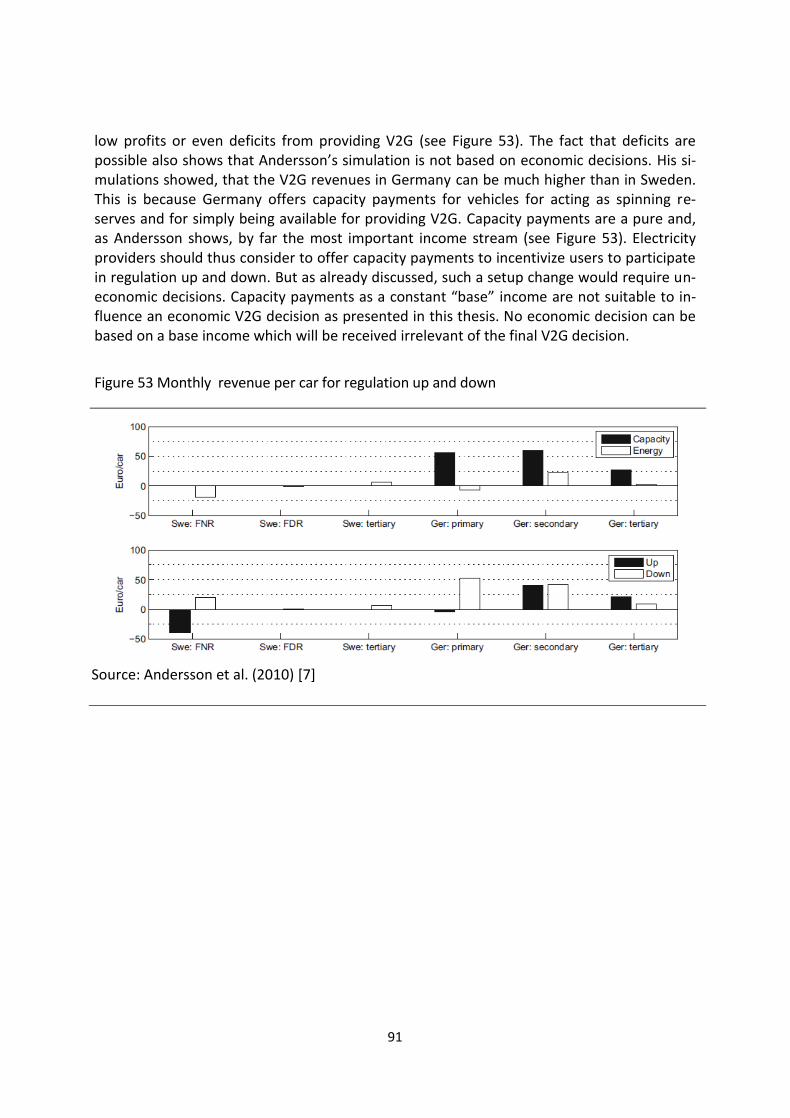
91
low profits or even deficits from providing V2G (see Figure 53). The fact that deficits are possible also shows that Andersson’s simulation is not based on economic decisions. His si-mulations showed, that the V2G revenues in Germany can be much higher than in Sweden. This is because Germany offers capacity payments for vehicles for acting as spinning re-serves and for simply being available for providing V2G. Capacity payments are a pure and, as Andersson shows, by far the most important income stream (see Figure 53). Electricity providers should thus consider to offer capacity payments to incentivize users to participate in regulation up and down. But as already discussed, such a setup change would require un-economic decisions. Capacity payments as a constant “base” income are not suitable to in-fluence an economic V2G decision as presented in this thesis. No economic decision can be based on a base income which will be received irrelevant of the final V2G decision.
Figure 53 Monthly revenue per car for regulation up and down
Source: Andersson et al. (2010) [7]
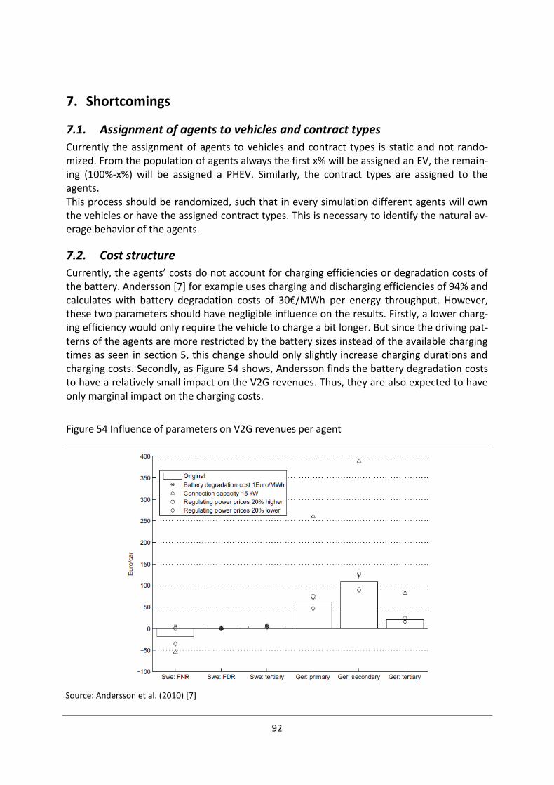
92
7. Shortcomings
7.1. Assignment of agents to vehicles and contract types
Currently the assignment of agents to vehicles and contract types is static and not rando-mized. From the population of agents always the first x% will be assigned an EV, the remain-ing (100%-x%) will be assigned a PHEV. Similarly, the contract types are assigned to the agents. This process should be randomized, such that in every simulation different agents will own the vehicles or have the assigned contract types. This is necessary to identify the natural av-erage behavior of the agents.
7.2. Cost structure
Currently, the agents’ costs do not account for charging efficiencies or degradation costs of the battery. Andersson [7] for example uses charging and discharging efficiencies of 94% and calculates with battery degradation costs of 30€/MWh per energy throughput. However, these two parameters should have negligible influence on the results. Firstly, a lower charg-ing efficiency would only require the vehicle to charge a bit longer. But since the driving pat-terns of the agents are more restricted by the battery sizes instead of the available charging times as seen in section 5, this change should only slightly increase charging durations and charging costs. Secondly, as Figure 54 shows, Andersson finds the battery degradation costs to have a relatively small impact on the V2G revenues. Thus, they are also expected to have only marginal impact on the charging costs.
Figure 54 Influence of parameters on V2G revenues per agent
Source: Andersson et al. (2010) [7]
93
7.3. Optimization
SOC limits Restricting the SOC of EVs to be within 10-90% and of PHEVs below 90% of the battery ca-pacity underestimates the vehicle’s range. This rigid setup does not allow the SOC to go a bit below or beyond the limits which is unrealistic. In reality, the vehicle should be able to con-tinue charging to 100% or discharging to 0% in extreme cases. In return, higher costs can be attributed for going beyond the limits. To solve this more complex problem, a one step solu-tion is not sufficient any more. Every agent should go through an iterative process. After the first assignment of charging times, it should be checked in which intervals the agent has an SOC below 10% or above 90%. For these times, the agent’s personal price function can be altered to reflect the “higher” battery costs. The charging times can then be determined again with linear pro-gramming. This iteration can be repeated until the agent’s plan cannot significantly improve its plan any further. Improvement of the Decentralized Smart Charging Algorithm Two improvements should be made to optimize the choice of charging times and to mitigate overcharging. First, as sections 5.2.2 and 6.1. suggest a long term agent planning and re-planning can greatly improve the scheduling of charging times globally. Second, a limit, λ, should be imposed on the amount of energy that agents can overcharge ((30) and (31)). Giving agents the freedom and flexibility to charge as much energy as they want, can result in additional peak loads instead of an optimal load flattening effect. In fact, the factor, λ, should be derived directly from the free load curve which defines the total energy available for charging. The total available energy which is pre-allocated for vehicle charging in the system is the integral over the free load curve in the ranges where the do-main of the free load function is positive ((32) and (33)).
)0),(max()( tfto (32)
dto
dayin seconds
0day over the [J]energy available total (33)
The total available energy is linked to the actual total energy need for n agents (34) by rela-tion (35). Thus, λ can be calculated using (36).
n
i
mptionTotalConsuE1
agents all of needenergy total (34)
dtoEn
i
mptionTotalConsu
dayin seconds
01
)1(* (35)
1
1
dayin seconds
0
n
i
mptionTotalConsuE
dto (36)

94
It might be questionable, if such a contract type can be sold in real life. Agents can be ex-pected to prefer a constantly fully charged battery regardless of their plans. Yet, an “egois-tic” charging decision without a limit on the maximum charging amount can only be possi-ble, if far more energy than actually needed is pre-allocated for charging with the free load curves. Yet, one may argue, that wasteful energy consumption should not be encouraged in a resource restricted world.
7.4. Agent decision
The developed module does not give feed back to the MATSim iteration to influence the agent’s plans or choices. However the charging optimization can give hints, (i) if the agent’s mode choice is suitable and (ii) if his personal plans can work better by prolonging his park-ing and charging duration or by choosing a parking location with a fast speed charging infra-structure. In the first case, an exit flag can indicate if the mode choice of the agent is not suitable. Since it is known how much energy was used from the battery or from other sources (com-bustion engine or battery swap) it is clear, if the agent’s trip is much longer than the vehicles range. In this case, the agent should definitely switch to a PHEV or to yet another transport option if he is driving an EV. In the second case, notice should be given if the SOC of the agent falls below the minimum of 10%. In these cases, the charging time in the previous parking interval should be pro-longed or an additional stop at a speed charging station could be arranged in the next itera-tion, if in range. For these two cases, exit flags need to be defined, which can then help to optimize the agent’s plans.
95
8. Conclusion This thesis successfully implements a decentralized smart charging and V2G simulation with-in the large scale traffic modeling software MATSim. It is seen, that the battery size has the largest impact on the simulation results. The battery size directly determines the failure rate of electric vehicles, respectively the need for PHEVs to use their combustion engine which generates emissions. It also significantly influences charging durations and costs. Thus, a thorough consultancy for every buyer of an EV or PHEV based on their daily travel pattern seems a necessity to make a suitable vehicle choice. Surprisingly the gas price has no influence on the charging duration and only small effects on the total driving costs at the chosen rates. The ratio of EVs to PHEVs in the system has no influence on the charging behavior of the agents and only influences the total number of extra emissions in the system. Overall, the proposed decentralized smart charging algorithm is a suitable and promising al-ternative to centralized smart charging algorithms. The integration of continuous re-planning and a limit on overcharging for agents is suggested to mitigate grid violations and to reach the maximum load flattening effect. The solution functions well with minimal input to achieve global optimum without multiple iterations. However, the challenges for the actual implementation are (i) to estimate the predicted free load curve with reasonable accuracy and (ii) to synchronize or update the free load curve in every vehicle in case of severe grid violations. Furthermore, it is shown that the V2G regulation potential of vehicles under the proposed set up is very limited, the optimization very restrictive and largely not an economic decision. EVs and PHEVs have similar regulation down capacities and again similar regulation up ca-pacities if the participation rate in regulation up is 100%. Further simulations are needed to determine, whether the slight variations of regulation up behavior at lower penetrations of regulation up contracts observed are specific to EVs or PHEVs or are influenced by the cur-rent set up of assigning contract types and vehicles to agents. In spite of the similar regulation capacities, the V2G revenues for EVs and PHEVs differ. EVs and PHEVs receive comparable revenues from direct compensation payments, however the scheduling flexibility of PHEVs results in on average significantly higher saving opportunities from indirect savings from rescheduling for PHEVs. This makes V2G generally more attrac-tive for PHEVs. However, at the current compensation rates and the low regulation potential of both EVs and PHEVs, participation in V2G is by no means a lucrative income stream. To actually en-courage or implement V2G today, firstly, the introduction of capacity payments is impor-tant. Secondly, contract types will have to implemented in which vehicles cannot make purely economic decisions. This setup limits V2G to PHEVs.

I
9 Acknowledgements First of all, I would like to thank Prof. Dr. Axhausen for giving me the opportunity to be part of this project and to build on the large scale simulation framework MATSim. I would also like to thank my supervisor, Rashid Waraich, for his technical assistance and feedback.
I
10 Bibliography [1] URL: http://www.autobild.de/artikel/serienstart-subaru-stella-ev-917625.html
Accessed: October 2009
[2] MATSim-T: Multi Agent Transportation Simulation Toolkit (2008), URL: http://www.matsim.org
[3] Röthlisberger, R. and M. Weibel, Schweizer Klimapolitik auf einen Blick - Kurzfassung des klimapolitischen Berichts 2009 der Schweiz an das UNO-Klimasekretariat, Bundesamt für Umwelt (BAFU), Bern.
[4] Waraich, R.A., M.D. Galus, C. Dobler, M. Balmer, G. Andersson, and K.W. Axhausen (2009) Plug-in Hybrid Electric Vehicles and Smart Grid : Investigations Based on a Micro- Simulation, 12th International Conference on Travel Behaviour Research (IATBR), Jaipur, India.
[5] Duckham, M. and R. Bennett (2009) Ambient Spatial Intelligence, Behavior monitor-ing and interpretation, B. Gottfried and H. Aghajan, eds., Amsterdam, Netherlands: IOS Press, 319-335.
[6] Schieffer, S.V. (2010), To charge or not to charge? Decentralized charging decisions for the smart grid, Semester thesis, ETH Zürich, Zurich.
[7] Andersson, S.-L., A.K. Elofsson, M.D. Galus, L. Göransson, S. Karlsson, F. Johnsson, and G. Andersson (2010) Plug-in hybrid electric vehicles as regulating power provid-ers: Case studies of Sweden and Germany, Energy Policy, 38, 2751-2762.
[8] Kempton, W. and J. Tomic (2005) Vehicle-to-grid power fundamentals: Calculating capacity and net revenue, Journal of Power Sources, 144, 268-279.
[9] Larsen, D.K., E. Chandrashekhara and J. Ostergard, (2008) Electric vehicles for im-proved operation of power systems with high wind power penetration, IEEE Energy 2030, Atlanta, GA, USA.
[10] Holland, J.H. (1992) Adaptation in Natural and Artificial Systems: An Introductory Analysis with Applications to Biology, MIT Press. Cambridge, MA, USA.
[11] LPSolve (2010) http://lpsolve.sourceforge.net. Accessed: March 2011.
[12] URL: http://gasbuddy.com, Accessed: June 2011.
[13] URL: http://tanktip.ch, Accessed: June 2011.
[14] URL: http://de.wikipedia.org/wiki/Motorenbenzin, Accessed: June 2011.
[15] Vytelingum, P., T.D. Voice, S.D. Ramchurn, A. Rogers, and N.R. Jennings (2010) Agent-based Micro-Storage Management for the Smart Grid, Proceedings of 9th In-ternational Conference on Autonomous Agents and Multiagent Systems (AAMAS 2010), Toronto, Canada.
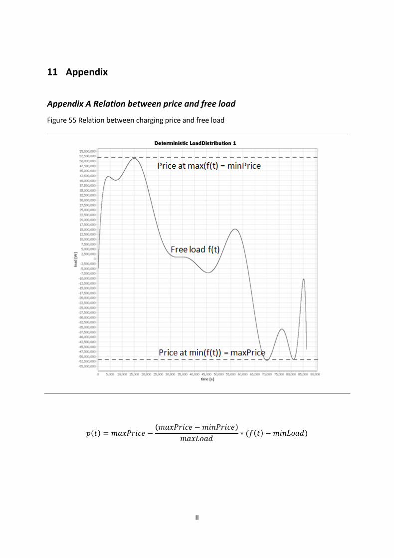
II
11 Appendix
Appendix A Relation between price and free load
Figure 55 Relation between charging price and free load

III
Appendix B Hub Mapping
To be able to simulate different load profiles in different areas or different price policies, multiple hubs can be defined in the simulation. Finally links can be assigned to these hubs. In the current setup (Class StellasHubMapping), the number of hubs in x and y direction can be chosen by the user. The minimum and maximum coordinates of the links in the network are determined. The resulting bounding area ((xmin, ymin), (xmax, ymin), (xmax, ymax), (xmin, ymax )) is then divided into rectangular areas corresponding to the number of hubs in x and y direction. I.e. if there are two hubs in x direction the first hubs will span between
to
and the second hub between
to . If
there is one hub in y direction it will span between to . Figure 56 shows an ex-ample. To assign the links to the hub, the location of their center of mass is used to determine to which hub they belong. Links that pass through multiple hubs are thus assigned to the hub in which their center of gravity lies (i.e. the dashed links in Figure 56 are assigned to hub 2). Functionality Test Setup The first test simulation simply checks, if the different hubs with different price policies real-ly do produce different charging costs for the agents. For this purpose, the institute test sce-nario is used and the network is divided into two hubs (network divided into 2 hubs in x and 1 hub in y direction). The first hub has regular electricity costs of 0.07CHF/kWh in off peak and 0.11CHF/kWh in peak times. The second hub has prices of 50-100 CHF/kWh. Expected Outcome It is expected that agents travelling in or partly within hub 2 have significantly higher aver-age charging costs than those who only travel in hub 1. This difference in charging costs can then later be exploited to alter decisions of agents and to use alternate routes or choose al-ternate work or shopping locations to reduce their costs. Results The test confirmed that the code is working correctly. The average cost for agents travelling partly or completely within the hub with the high charging costs were a factor of 730 greater than for those agents only travelling in the hub with the regular charging costs. Average cost for agents of 1.69 CHF at hub 1 Average cost for agents of 1234.25 CHF at hub 2
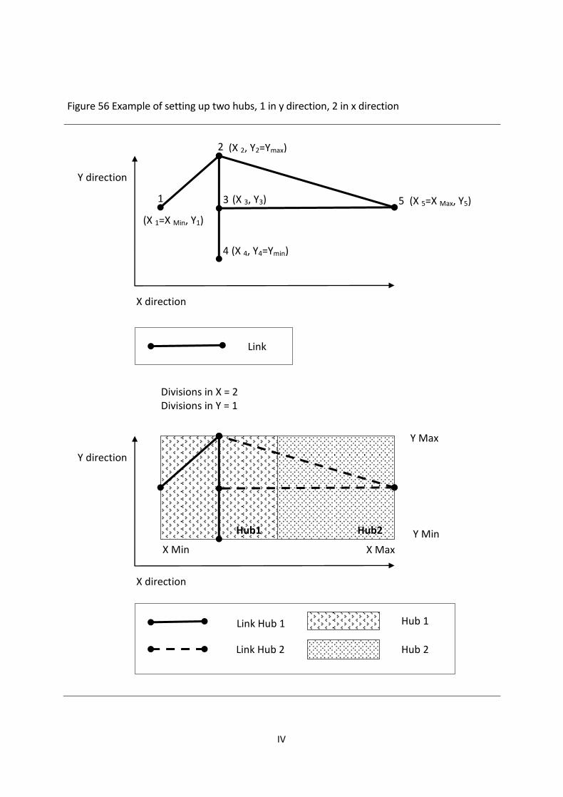
IV
Figure 56 Example of setting up two hubs, 1 in y direction, 2 in x direction
Divisions in X = 2 Divisions in Y = 1
X direction
Y direction
X Min X Max
Y Max
Y Min Hub1 Hub2
Link Hub 1 Hub 1
Link Hub 2 Hub 2
X direction
Y direction
(X 1=X Min, Y1)
(X 5=X Max, Y5)
Link
1
2
3
4
5
(X 4, Y4=Ymin)
(X 2, Y2=Ymax)
(X 3, Y3)
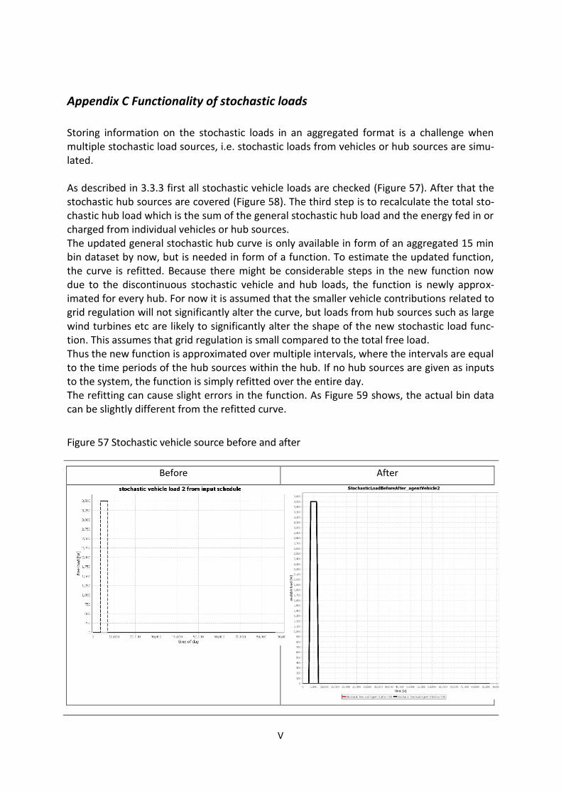
V
Appendix C Functionality of stochastic loads
Storing information on the stochastic loads in an aggregated format is a challenge when multiple stochastic load sources, i.e. stochastic loads from vehicles or hub sources are simu-lated. As described in 3.3.3 first all stochastic vehicle loads are checked (Figure 57). After that the stochastic hub sources are covered (Figure 58). The third step is to recalculate the total sto-chastic hub load which is the sum of the general stochastic hub load and the energy fed in or charged from individual vehicles or hub sources. The updated general stochastic hub curve is only available in form of an aggregated 15 min bin dataset by now, but is needed in form of a function. To estimate the updated function, the curve is refitted. Because there might be considerable steps in the new function now due to the discontinuous stochastic vehicle and hub loads, the function is newly approx-imated for every hub. For now it is assumed that the smaller vehicle contributions related to grid regulation will not significantly alter the curve, but loads from hub sources such as large wind turbines etc are likely to significantly alter the shape of the new stochastic load func-tion. This assumes that grid regulation is small compared to the total free load. Thus the new function is approximated over multiple intervals, where the intervals are equal to the time periods of the hub sources within the hub. If no hub sources are given as inputs to the system, the function is simply refitted over the entire day. The refitting can cause slight errors in the function. As Figure 59 shows, the actual bin data can be slightly different from the refitted curve.
Figure 57 Stochastic vehicle source before and after
Before After
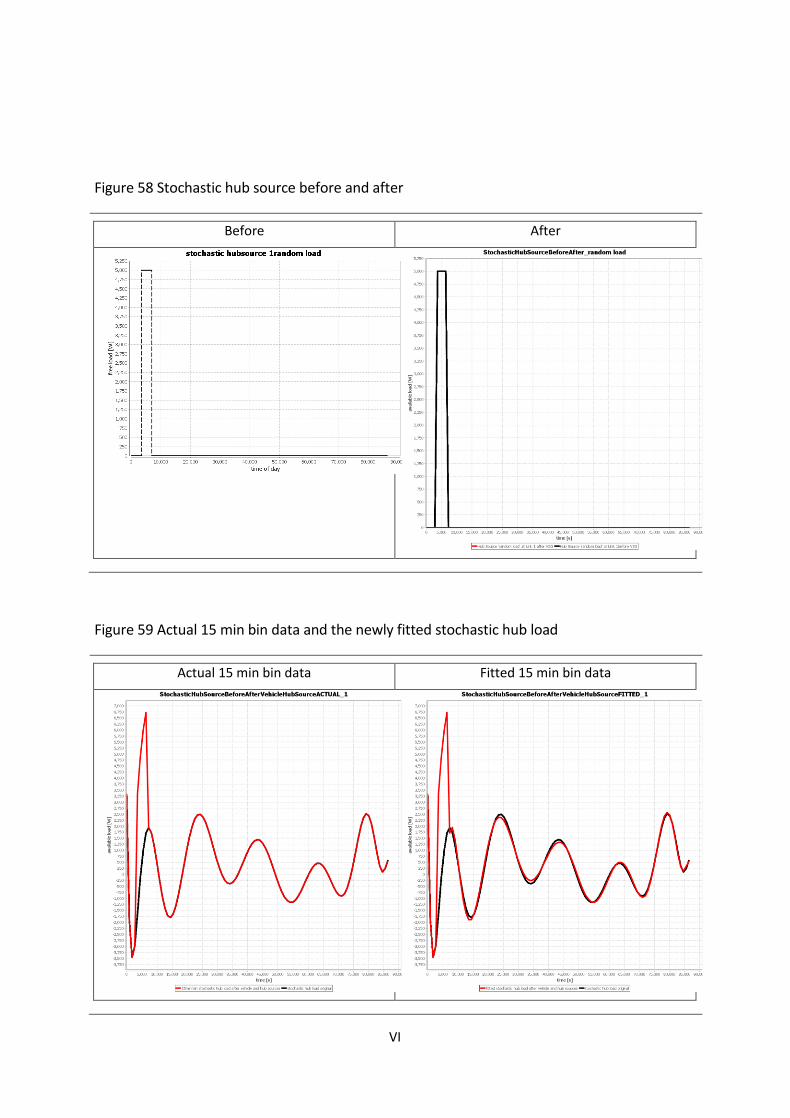
VI
Figure 58 Stochastic hub source before and after
Before After
Figure 59 Actual 15 min bin data and the newly fitted stochastic hub load
Actual 15 min bin data Fitted 15 min bin data

VII
Appendix D V2G Cutoff Percentage
To save time the V2G calculation is only made for a vehicle, if the requested energy is above a minimum threshold. Because the input stochastic load was chose between -5000W to 5000W and since there are 16000 agents in the system, it is calculated that:
The minimum cut off threshold is thus chosen as x= 0.00001. This will certainly not capture the entire possible V2G potential, but going below 0.001% of the connection capacity is highly unrealistic.
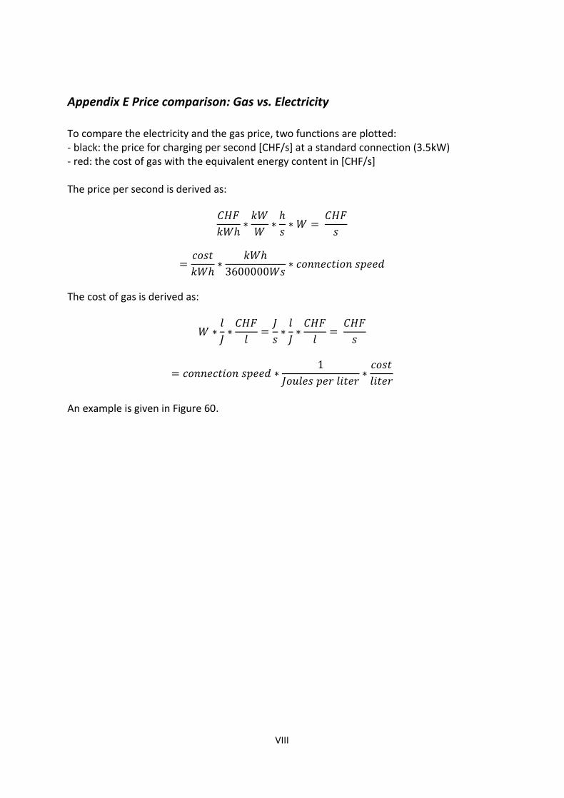
VIII
Appendix E Price comparison: Gas vs. Electricity
To compare the electricity and the gas price, two functions are plotted: - black: the price for charging per second [CHF/s] at a standard connection (3.5kW) - red: the cost of gas with the equivalent energy content in [CHF/s] The price per second is derived as:
The cost of gas is derived as:
An example is given in Figure 60.
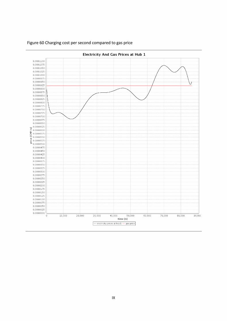
IX
Figure 60 Charging cost per second compared to gas price
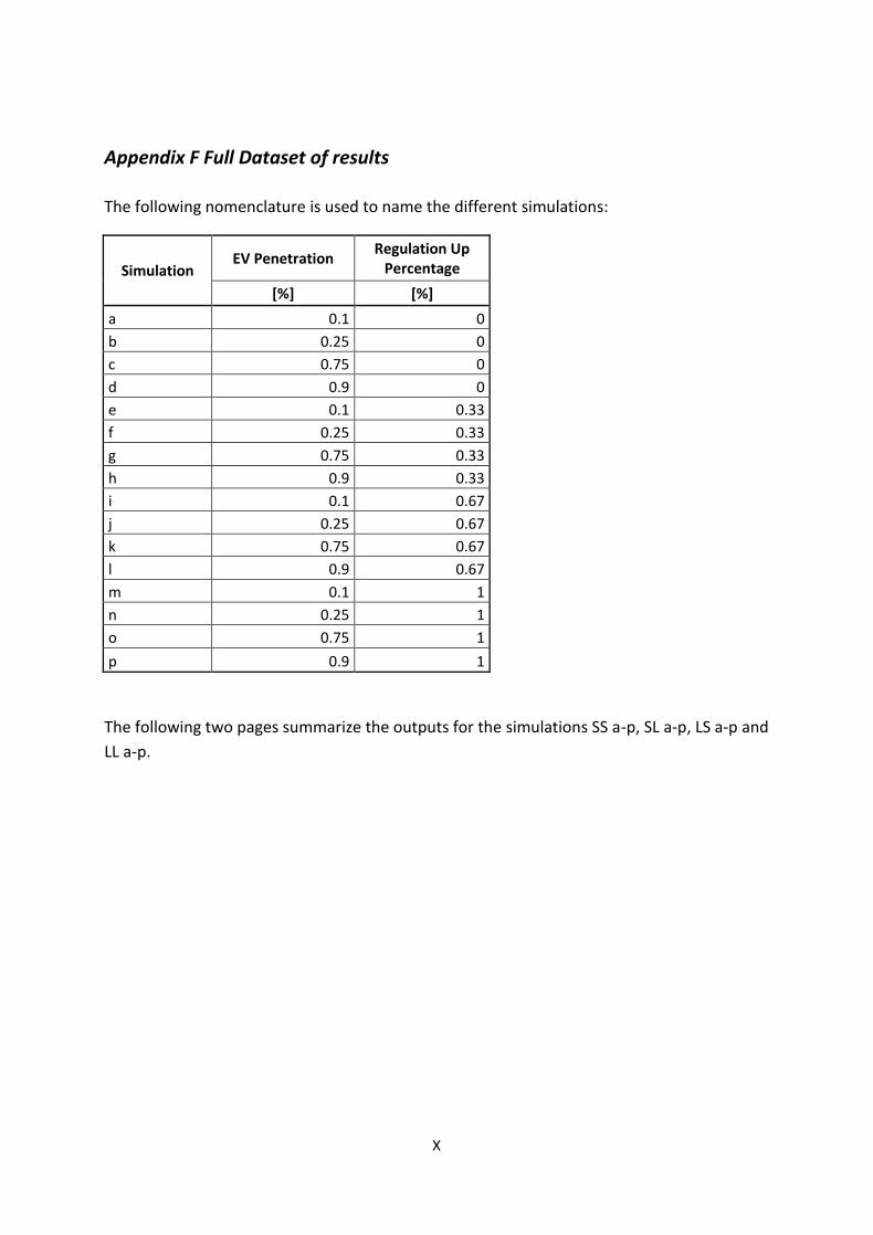
X
Appendix F Full Dataset of results
The following nomenclature is used to name the different simulations:
Simulation EV Penetration
Regulation Up Percentage
[%] [%]
a 0.1 0
b 0.25 0
c 0.75 0
d 0.9 0
e 0.1 0.33
f 0.25 0.33
g 0.75 0.33
h 0.9 0.33
i 0.1 0.67
j 0.25 0.67
k 0.75 0.67
l 0.9 0.67
m 0.1 1
n 0.25 1
o 0.75 1
p 0.9 1
The following two pages summarize the outputs for the simulations SS a-p, SL a-p, LS a-p and
LL a-p.
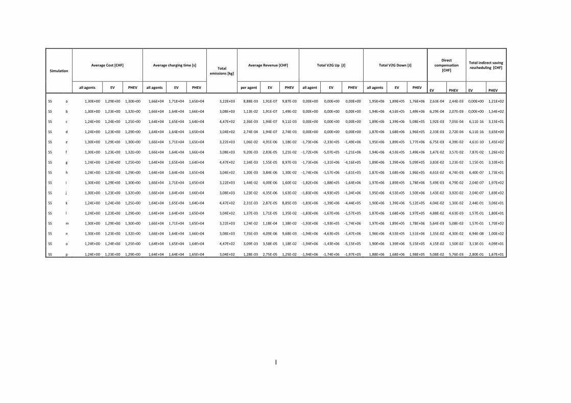
I
Simulation
Average Cost [CHF] Average charging time [s] Total
emissions [kg]
Average Revenue [CHF] Total V2G Up [J] Total V2G Down [J] Direct
compensation [CHF]
Total indirect saving rescheduling [CHF]
all agents EV PHEV all agents EV PHEV per agent EV PHEV all agent EV PHEV all agents EV PHEV EV PHEV EV PHEV
SS a 1,30E+00 1,29E+00 1,30E+00 1,66E+04 1,71E+04 1,65E+04 3,22E+03 8,88E-03 1,91E-07 9,87E-03 0,00E+00 0,00E+00 0,00E+00 1,95E+06 1,89E+05 1,76E+06 2,63E-04 2,44E-03 0,00E+00 1,21E+02
SS b 1,30E+00 1,23E+00 1,32E+00 1,66E+04 1,64E+04 1,66E+04 3,08E+03 1,13E-02 1,91E-07 1,49E-02 0,00E+00 0,00E+00 0,00E+00 1,94E+06 4,53E+05 1,49E+06 6,29E-04 2,07E-03 0,00E+00 1,54E+02
SS c 1,24E+00 1,24E+00 1,25E+00 1,64E+04 1,65E+04 1,64E+04 4,47E+02 2,36E-03 1,94E-07 9,11E-03 0,00E+00 0,00E+00 0,00E+00 1,89E+06 1,39E+06 5,08E+05 1,92E-03 7,05E-04 6,11E-16 3,15E+01
SS d 1,24E+00 1,23E+00 1,29E+00 1,64E+04 1,64E+04 1,65E+04 3,04E+02 2,74E-04 1,94E-07 2,74E-03 0,00E+00 0,00E+00 0,00E+00 1,87E+06 1,68E+06 1,96E+05 2,33E-03 2,72E-04 6,11E-16 3,65E+00
SS e 1,30E+00 1,29E+00 1,30E+00 1,66E+04 1,71E+04 1,65E+04 3,22E+03 1,06E-02 4,91E-06 1,18E-02 -1,73E+06 -2,33E+05 -1,49E+06 1,95E+06 1,89E+05 1,77E+06 6,75E-03 4,39E-02 4,61E-10 1,45E+02
SS f 1,30E+00 1,23E+00 1,32E+00 1,66E+04 1,64E+04 1,66E+04 3,08E+03 9,20E-03 2,83E-05 1,21E-02 -1,72E+06 -5,07E+05 -1,21E+06 1,94E+06 4,53E+05 1,49E+06 1,47E-02 3,57E-02 7,87E-02 1,26E+02
SS g 1,24E+00 1,24E+00 1,25E+00 1,64E+04 1,65E+04 1,64E+04 4,47E+02 2,34E-03 1,55E-05 8,97E-03 -1,73E+06 -1,31E+06 -4,16E+05 1,89E+06 1,39E+06 5,09E+05 3,83E-02 1,23E-02 1,15E-01 3,10E+01
SS h 1,24E+00 1,23E+00 1,29E+00 1,64E+04 1,64E+04 1,65E+04 3,04E+02 1,30E-03 3,84E-06 1,30E-02 -1,74E+06 -1,57E+06 -1,61E+05 1,87E+06 1,68E+06 1,96E+05 4,61E-02 4,74E-03 6,40E-07 1,73E+01
SS i 1,30E+00 1,29E+00 1,30E+00 1,66E+04 1,71E+04 1,65E+04 3,22E+03 1,44E-02 4,00E-06 1,60E-02 -1,82E+06 -1,88E+05 -1,64E+06 1,97E+06 1,89E+05 1,78E+06 5,49E-03 4,79E-02 2,04E-07 1,97E+02
SS j 1,30E+00 1,23E+00 1,32E+00 1,66E+04 1,64E+04 1,66E+04 3,08E+03 1,23E-02 4,35E-06 1,63E-02 -1,83E+06 -4,93E+05 -1,34E+06 1,95E+06 4,53E+05 1,50E+06 1,43E-02 3,92E-02 2,04E-07 1,69E+02
SS k 1,24E+00 1,24E+00 1,25E+00 1,64E+04 1,65E+04 1,64E+04 4,47E+02 2,31E-03 2,87E-05 8,85E-03 -1,83E+06 -1,39E+06 -4,44E+05 1,90E+06 1,39E+06 5,12E+05 4,04E-02 1,30E-02 2,44E-01 3,06E+01
SS l 1,24E+00 1,23E+00 1,29E+00 1,64E+04 1,64E+04 1,65E+04 3,04E+02 1,37E-03 1,71E-05 1,35E-02 -1,83E+06 -1,67E+06 -1,57E+05 1,87E+06 1,68E+06 1,97E+05 4,88E-02 4,63E-03 1,57E-01 1,80E+01
SS m 1,30E+00 1,29E+00 1,30E+00 1,66E+04 1,71E+04 1,65E+04 3,22E+03 1,24E-02 1,18E-04 1,38E-02 -1,93E+06 -1,93E+05 -1,74E+06 1,97E+06 1,89E+05 1,78E+06 5,64E-03 5,08E-02 1,57E-01 1,70E+02
SS n 1,30E+00 1,23E+00 1,32E+00 1,66E+04 1,64E+04 1,66E+04 3,08E+03 7,35E-03 4,09E-06 9,68E-03 -1,94E+06 -4,63E+05 -1,47E+06 1,96E+06 4,53E+05 1,51E+06 1,35E-02 4,30E-02 6,94E-08 1,00E+02
SS o 1,24E+00 1,24E+00 1,25E+00 1,64E+04 1,65E+04 1,64E+04 4,47E+02 3,09E-03 3,58E-05 1,18E-02 -1,94E+06 -1,43E+06 -5,15E+05 1,90E+06 1,39E+06 5,15E+05 4,15E-02 1,50E-02 3,13E-01 4,09E+01
SS p 1,24E+00 1,23E+00 1,29E+00 1,64E+04 1,64E+04 1,65E+04 3,04E+02 1,28E-03 2,75E-05 1,25E-02 -1,94E+06 -1,74E+06 -1,97E+05 1,88E+06 1,68E+06 1,98E+05 5,08E-02 5,76E-03 2,80E-01 1,67E+01
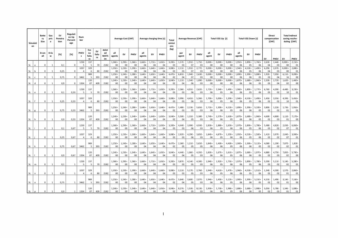
I
Simulation
Battery
Size
Gas pric
e
EV Penetra
tion
Regulation Up
Percentage
Number
Average Cost [CHF] Average charging time [s] Total
emissions [kg]
Average Revenue [CHF] Total V2G Up [J] Total V2G Down [J] Direct
compensation [CHF]
Total indirect saving resche-duling [CHF]
0=small
0=low
[%] [%] PHEV
s
Evs no
failure
EV failu
re
deleted
MATSim
all agents
EV PHEV all
agents EV PHEV
per agent
EV PHEV all
agent EV PHEV
all agents
EV PHEV
EV PHEV EV PHEV
SL a 0 1 0,1 0 1230
5 137
5 70 2182 1,36E+
00 1,29E+
00 1,36E+
00 1,66E+
04 1,71E+
04 1,65E+
04 3,20E+
03 1,57E-
03 1,91E-
07 1,75E-
03 0,00E+
00 0,00E+
00 0,00E+
00 1,95E+
06 1,89E+
05 1,76E+
06 2,63E-
04 2,44E-
03 0,00E+
00 2,15E+
01
SL b 0 1 0,25 0 1037
4 329
6 80 2182 1,35E+
00 1,23E+
00 1,39E+
00 1,66E+
04 1,64E+
04 1,66E+
04 3,08E+
03 2,11E-
03 1,91E-
07 2,77E-
03 0,00E+
00 0,00E+
00 0,00E+
00 1,94E+
06 4,53E+
05 1,49E+
06 6,29E-
04 2,07E-
03 0,00E+
00 2,88E+
01
SL c 0 1 0,75 0 3462 989
5 393 2182 1,25E+
00 1,24E+
00 1,28E+
00 1,64E+
04 1,65E+
04 1,64E+
04 4,47E+
02 6,81E-
04 1,94E-
07 2,63E-
03 0,00E+
00 0,00E+
00 0,00E+
00 1,89E+
06 1,39E+
06 5,08E+
05 1,92E-
03 7,05E-
04 6,11E-
16 9,09E+
00
SL d 0 1 0,9 0 1334 120
07 409 2182 1,24E+
00 1,23E+
00 1,34E+
00 1,64E+
04 1,64E+
04 1,65E+
04 3,04E+
02 1,11E-
04 1,54E-
06 1,09E-
03 0,00E+
00 0,00E+
00 0,00E+
00 1,87E+
06 1,68E+
06 1,96E+
05 2,33E-
03 2,72E-
04 1,62E-
02 1,46E+
00
SL e 0 1 0,1 0,33 1230
5 137
5 70 2182 1,36E+
00 1,29E+
00 1,36E+
00 1,66E+
04 1,71E+
04 1,65E+
04 3,20E+
03 2,36E-
03 4,91E-
06 2,62E-
03
-1,72E+
06
-2,34E+
05
-1,49E+
06 1,96E+
06 1,89E+
05 1,77E+
06 6,76E-
03 4,39E-
02 4,48E-
10 3,23E+
01
SL f 0 1 0,25 0,33 1037
4 329
6 80 2182 1,35E+
00 1,23E+
00 1,39E+
00 1,66E+
04 1,64E+
04 1,66E+
04 3,08E+
03 3,99E-
03 4,41E-
06 5,26E-
03
-1,70E+
06
-5,00E+
05
-1,20E+
06 1,94E+
06 4,53E+
05 1,49E+
06 1,45E-
02 3,55E-
02 4,39E-
10 5,45E+
01
SL g 0 1 0,75 0,33 3462 989
5 393 2182 1,25E+
00 1,24E+
00 1,28E+
00 1,64E+
04 1,65E+
04 1,64E+
04 4,47E+
02 1,48E-
03 2,13E-
05 5,65E-
03
-1,71E+
06
-1,30E+
06
-4,12E+
05 1,89E+
06 1,39E+
06 5,10E+
05 3,80E-
02 1,22E-
02 1,73E-
01 1,95E+
01
SL h 0 1 0,9 0,33 1334 120
07 409 2182 1,24E+
00 1,23E+
00 1,34E+
00 1,64E+
04 1,64E+
04 1,65E+
04 3,04E+
02 5,50E-
04 1,31E-
05 5,38E-
03
-1,74E+
06
-1,57E+
06
-1,63E+
05 1,87E+
06 1,68E+
06 1,96E+
05 4,60E-
02 4,80E-
03 1,11E-
01 7,17E+
00
SL i 0 1 0,1 0,67 1230
5 137
5 70 2182 1,36E+
00 1,29E+
00 1,36E+
00 1,66E+
04 1,71E+
04 1,65E+
04 3,20E+
03 4,44E-
03 3,99E-
06 4,93E-
03
-1,83E+
06
-1,88E+
05
-1,65E+
06 1,97E+
06 1,89E+
05 1,78E+
06 5,48E-
03 4,82E-
02 2,03E-
07 6,06E+
01
SL j 0 1 0,25 0,67 1037
4 329
6 80 2182 1,35E+
00 1,23E+
00 1,39E+
00 1,66E+
04 1,64E+
04 1,66E+
04 3,08E+
03 2,92E-
03 4,29E-
06 3,85E-
03
-1,84E+
06
-4,87E+
05
-1,35E+
06 1,95E+
06 4,53E+
05 1,50E+
06 1,41E-
02 3,97E-
02 2,04E-
07 3,99E+
01
SL k 0 1 0,75 0,67 3462 989
5 393 2182 1,25E+
00 1,24E+
00 1,28E+
00 1,64E+
04 1,65E+
04 1,64E+
04 4,47E+
02 2,36E-
05 1,21E-
05 5,65E-
05
-1,84E+
06
-1,40E+
06
-4,40E+
05 1,90E+
06 1,39E+
06 5,12E+
05 4,08E-
02 1,29E-
02 7,87E-
02 1,83E-
01
SL l 0 1 0,9 0,67 1334 120
07 409 2182 1,24E+
00 1,23E+
00 1,34E+
00 1,64E+
04 1,64E+
04 1,65E+
04 3,04E+
02 4,44E-
04 1,06E-
05 4,35E-
03
-1,83E+
06
-1,67E+
06
-1,61E+
05 1,87E+
06 1,68E+
06 1,97E+
05 4,88E-
02 4,75E-
03 7,85E-
02 5,79E+
00
SL m 0 1 0,1 1 1230
5 137
5 70 2182 1,36E+
00 1,29E+
00 1,36E+
00 1,66E+
04 1,71E+
04 1,65E+
04 3,20E+
03 3,87E-
03 4,14E-
05 4,30E-
03
-1,94E+
06
-1,92E+
05
-1,75E+
06 1,97E+
06 1,89E+
05 1,78E+
06 5,59E-
03 5,11E-
02 5,14E-
02 5,28E+
01
SL n 0 1 0,25 1 1037
4 329
6 80 2182 1,35E+
00 1,23E+
00 1,39E+
00 1,66E+
04 1,64E+
04 1,66E+
04 3,08E+
03 2,11E-
03 5,17E-
05 2,76E-
03
-1,94E+
06
-4,61E+
05
-1,47E+
06 1,96E+
06 4,53E+
05 1,51E+
06 1,34E-
02 4,30E-
02 1,57E-
01 2,86E+
01
SL o 0 1 0,75 1 3462 989
5 393 2182 1,25E+
00 1,24E+
00 1,28E+
00 1,64E+
04 1,65E+
04 1,64E+
04 4,47E+
02 5,64E-
04 3,60E-
05 2,07E-
03
-1,94E+
06
-1,43E+
06
-5,12E+
05 1,90E+
06 1,39E+
06 5,15E+
05 4,15E-
02 1,49E-
02 3,14E-
01 7,16E+
00
SL p 0 1 0,9 1 1334 120
07 409 2182 1,24E+
00 1,23E+
00 1,34E+
00 1,64E+
04 1,64E+
04 1,65E+
04 3,04E+
02 8,27E-
04 1,53E-
05 8,13E-
03
-1,93E+
06
-1,73E+
06
-1,98E+
05 1,88E+
06 1,68E+
06 1,98E+
05 5,05E-
02 5,78E-
03 1,34E-
01 1,08E+
01
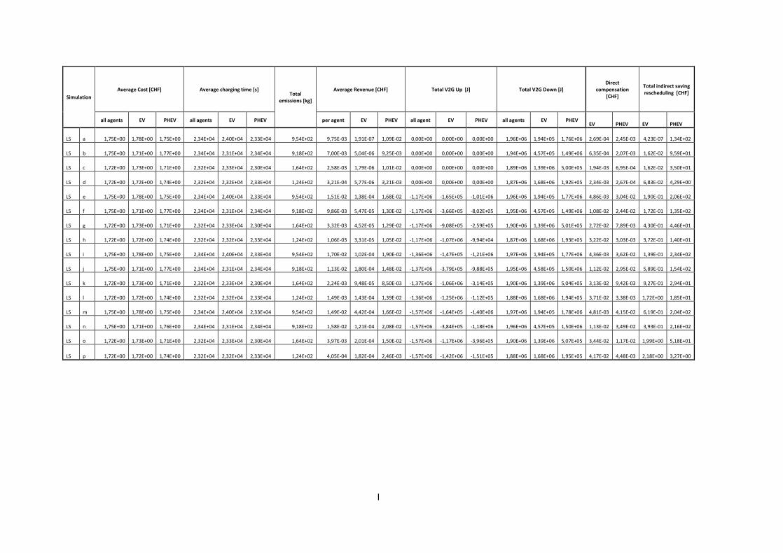
I
Simulation
Average Cost [CHF] Average charging time [s] Total
emissions [kg]
Average Revenue [CHF] Total V2G Up [J] Total V2G Down [J] Direct
compensation [CHF]
Total indirect saving rescheduling [CHF]
all agents EV PHEV all agents EV PHEV per agent EV PHEV all agent EV PHEV all agents EV PHEV EV PHEV EV PHEV
LS a 1,75E+00 1,78E+00 1,75E+00 2,34E+04 2,40E+04 2,33E+04 9,54E+02 9,75E-03 1,91E-07 1,09E-02 0,00E+00 0,00E+00 0,00E+00 1,96E+06 1,94E+05 1,76E+06 2,69E-04 2,45E-03 4,23E-07 1,34E+02
LS b 1,75E+00 1,71E+00 1,77E+00 2,34E+04 2,31E+04 2,34E+04 9,18E+02 7,00E-03 5,04E-06 9,25E-03 0,00E+00 0,00E+00 0,00E+00 1,94E+06 4,57E+05 1,49E+06 6,35E-04 2,07E-03 1,62E-02 9,59E+01
LS c 1,72E+00 1,73E+00 1,71E+00 2,32E+04 2,33E+04 2,30E+04 1,64E+02 2,58E-03 1,79E-06 1,01E-02 0,00E+00 0,00E+00 0,00E+00 1,89E+06 1,39E+06 5,00E+05 1,94E-03 6,95E-04 1,62E-02 3,50E+01
LS d 1,72E+00 1,72E+00 1,74E+00 2,32E+04 2,32E+04 2,33E+04 1,24E+02 3,21E-04 5,77E-06 3,21E-03 0,00E+00 0,00E+00 0,00E+00 1,87E+06 1,68E+06 1,92E+05 2,34E-03 2,67E-04 6,83E-02 4,29E+00
LS e 1,75E+00 1,78E+00 1,75E+00 2,34E+04 2,40E+04 2,33E+04 9,54E+02 1,51E-02 1,38E-04 1,68E-02 -1,17E+06 -1,65E+05 -1,01E+06 1,96E+06 1,94E+05 1,77E+06 4,86E-03 3,04E-02 1,90E-01 2,06E+02
LS f 1,75E+00 1,71E+00 1,77E+00 2,34E+04 2,31E+04 2,34E+04 9,18E+02 9,86E-03 5,47E-05 1,30E-02 -1,17E+06 -3,66E+05 -8,02E+05 1,95E+06 4,57E+05 1,49E+06 1,08E-02 2,44E-02 1,72E-01 1,35E+02
LS g 1,72E+00 1,73E+00 1,71E+00 2,32E+04 2,33E+04 2,30E+04 1,64E+02 3,32E-03 4,52E-05 1,29E-02 -1,17E+06 -9,08E+05 -2,59E+05 1,90E+06 1,39E+06 5,01E+05 2,72E-02 7,89E-03 4,30E-01 4,46E+01
LS h 1,72E+00 1,72E+00 1,74E+00 2,32E+04 2,32E+04 2,33E+04 1,24E+02 1,06E-03 3,31E-05 1,05E-02 -1,17E+06 -1,07E+06 -9,94E+04 1,87E+06 1,68E+06 1,93E+05 3,22E-02 3,03E-03 3,72E-01 1,40E+01
LS i 1,75E+00 1,78E+00 1,75E+00 2,34E+04 2,40E+04 2,33E+04 9,54E+02 1,70E-02 1,02E-04 1,90E-02 -1,36E+06 -1,47E+05 -1,21E+06 1,97E+06 1,94E+05 1,77E+06 4,36E-03 3,62E-02 1,39E-01 2,34E+02
LS j 1,75E+00 1,71E+00 1,77E+00 2,34E+04 2,31E+04 2,34E+04 9,18E+02 1,13E-02 1,80E-04 1,48E-02 -1,37E+06 -3,79E+05 -9,88E+05 1,95E+06 4,58E+05 1,50E+06 1,12E-02 2,95E-02 5,89E-01 1,54E+02
LS k 1,72E+00 1,73E+00 1,71E+00 2,32E+04 2,33E+04 2,30E+04 1,64E+02 2,24E-03 9,48E-05 8,50E-03 -1,37E+06 -1,06E+06 -3,14E+05 1,90E+06 1,39E+06 5,04E+05 3,13E-02 9,42E-03 9,27E-01 2,94E+01
LS l 1,72E+00 1,72E+00 1,74E+00 2,32E+04 2,32E+04 2,33E+04 1,24E+02 1,49E-03 1,43E-04 1,39E-02 -1,36E+06 -1,25E+06 -1,12E+05 1,88E+06 1,68E+06 1,94E+05 3,71E-02 3,38E-03 1,72E+00 1,85E+01
LS m 1,75E+00 1,78E+00 1,75E+00 2,34E+04 2,40E+04 2,33E+04 9,54E+02 1,49E-02 4,42E-04 1,66E-02 -1,57E+06 -1,64E+05 -1,40E+06 1,97E+06 1,94E+05 1,78E+06 4,81E-03 4,15E-02 6,19E-01 2,04E+02
LS n 1,75E+00 1,71E+00 1,76E+00 2,34E+04 2,31E+04 2,34E+04 9,18E+02 1,58E-02 1,21E-04 2,08E-02 -1,57E+06 -3,84E+05 -1,18E+06 1,96E+06 4,57E+05 1,50E+06 1,13E-02 3,49E-02 3,93E-01 2,16E+02
LS o 1,72E+00 1,73E+00 1,71E+00 2,32E+04 2,33E+04 2,30E+04 1,64E+02 3,97E-03 2,01E-04 1,50E-02 -1,57E+06 -1,17E+06 -3,96E+05 1,90E+06 1,39E+06 5,07E+05 3,44E-02 1,17E-02 1,99E+00 5,18E+01
LS p 1,72E+00 1,72E+00 1,74E+00 2,32E+04 2,32E+04 2,33E+04 1,24E+02 4,05E-04 1,82E-04 2,46E-03 -1,57E+06 -1,42E+06 -1,51E+05 1,88E+06 1,68E+06 1,95E+05 4,17E-02 4,48E-03 2,18E+00 3,27E+00

II
Simulation
Average Cost [CHF] Average charging time [s] Total emissions
[kg]
Average Revenue [CHF] Total V2G Up [J] Total V2G Down [J] Direct
compensation [CHF] Total indirect saving rescheduling [CHF]
all agents EV PHEV all agents EV PHEV per agent EV PHEV all agent EV PHEV all agents EV PHEV EV PHEV EV PHEV
LL a 1,78E+00 1,78E+00 1,78E+00 2,34E+04 2,40E+04 2,33E+04 9,56E+02 3,77E-03 1,83E-05 4,20E-03 0,00E+00 0,00E+00 0,00E+00 1,96E+06 1,94E+05 1,76E+06 2,69E-04 2,45E-03 2,56E-02 5,16E+01
LL b 1,77E+00 1,71E+00 1,79E+00 2,34E+04 2,31E+04 2,34E+04 9,19E+02 3,14E-03 1,90E-07 4,15E-03 0,00E+00 0,00E+00 0,00E+00 1,94E+06 4,57E+05 1,49E+06 6,35E-04 2,07E-03 6,17E-07 4,31E+01
LL c 1,73E+00 1,73E+00 1,73E+00 2,32E+04 2,33E+04 2,30E+04 1,64E+02 1,71E-04 1,92E-07 6,70E-04 0,00E+00 0,00E+00 0,00E+00 1,89E+06 1,39E+06 5,00E+05 1,94E-03 6,94E-04 3,76E-06 2,32E+00
LL d 1,72E+00 1,72E+00 1,76E+00 2,32E+04 2,32E+04 2,33E+04 1,24E+02 5,29E-04 2,84E-06 5,35E-03 0,00E+00 0,00E+00 0,00E+00 1,87E+06 1,68E+06 1,92E+05 2,33E-03 2,67E-04 3,23E-02 7,14E+00
LL e 1,78E+00 1,78E+00 1,78E+00 2,34E+04 2,40E+04 2,33E+04 9,56E+02 2,98E-03 1,82E-04 3,30E-03 -1,17E+06 -1,60E+05 -1,01E+06 1,96E+06 1,94E+05 1,77E+06 4,71E-03 3,04E-02 2,52E-01 4,06E+01
LL f 1,77E+00 1,71E+00 1,79E+00 2,34E+04 2,31E+04 2,34E+04 9,19E+02 3,66E-03 8,84E-05 4,81E-03 -1,17E+06 -3,61E+05 -8,12E+05 1,95E+06 4,57E+05 1,49E+06 1,07E-02 2,46E-02 2,84E-01 4,99E+01
LL g 1,73E+00 1,73E+00 1,73E+00 2,32E+04 2,33E+04 2,30E+04 1,64E+02 2,89E-04 6,29E-05 9,47E-04 -1,17E+06 -9,06E+05 -2,68E+05 1,89E+06 1,39E+06 5,01E+05 2,71E-02 8,14E-03 6,09E-01 3,27E+00
LL h 1,72E+00 1,72E+00 1,77E+00 2,32E+04 2,32E+04 2,33E+04 1,24E+02 4,17E-04 4,49E-05 3,82E-03 -1,17E+06 -1,07E+06 -9,97E+04 1,88E+06 1,68E+06 1,93E+05 3,21E-02 3,04E-03 5,18E-01 5,10E+00
LL i 1,78E+00 1,78E+00 1,78E+00 2,34E+04 2,40E+04 2,33E+04 9,56E+02 4,41E-03 5,18E-04 4,85E-03 -1,37E+06 -1,48E+05 -1,22E+06 1,97E+06 1,94E+05 1,77E+06 4,38E-03 3,63E-02 7,26E-01 5,97E+01
LL j 1,77E+00 1,71E+00 1,79E+00 2,34E+04 2,31E+04 2,34E+04 9,19E+02 3,15E-03 2,49E-04 4,09E-03 -1,37E+06 -3,78E+05 -9,92E+05 1,95E+06 4,58E+05 1,50E+06 1,11E-02 2,96E-02 8,20E-01 4,24E+01
LL k 1,73E+00 1,73E+00 1,73E+00 2,32E+04 2,33E+04 2,30E+04 1,64E+02 8,49E-04 9,53E-05 3,05E-03 -1,37E+06 -1,06E+06 -3,10E+05 1,90E+06 1,39E+06 5,04E+05 3,15E-02 9,30E-03 9,32E-01 1,05E+01
LL l 1,72E+00 1,72E+00 1,76E+00 2,32E+04 2,32E+04 2,33E+04 1,24E+02 1,91E-04 1,12E-04 9,08E-04 -1,37E+06 -1,25E+06 -1,16E+05 1,88E+06 1,68E+06 1,94E+05 3,71E-02 3,49E-03 1,34E+00 1,21E+00
LL m 1,78E+00 1,78E+00 1,78E+00 2,34E+04 2,40E+04 2,33E+04 9,56E+02 2,29E-03 4,58E-04 2,50E-03 -1,57E+06 -1,63E+05 -1,40E+06 1,97E+06 1,94E+05 1,78E+06 4,80E-03 4,15E-02 6,41E-01 3,07E+01
LL n 1,77E+00 1,71E+00 1,79E+00 2,34E+04 2,31E+04 2,34E+04 9,19E+02 2,06E-03 1,26E-04 2,68E-03 -1,56E+06 -3,84E+05 -1,18E+06 1,96E+06 4,57E+05 1,50E+06 1,13E-02 3,49E-02 4,10E-01 2,77E+01
LL o 1,73E+00 1,73E+00 1,73E+00 2,32E+04 2,33E+04 2,30E+04 1,64E+02 6,70E-04 1,26E-04 2,26E-03 -1,57E+06 -1,17E+06 -3,98E+05 1,90E+06 1,39E+06 5,07E+05 3,45E-02 1,18E-02 1,24E+00 7,80E+00
LL p 1,72E+00 1,72E+00 1,77E+00 2,32E+04 2,32E+04 2,33E+04 1,24E+02 2,13E-04 1,96E-04 3,63E-04 -1,57E+06 -1,41E+06 -1,54E+05 1,88E+06 1,68E+06 1,95E+05 4,16E-02 4,54E-03 2,36E+00 4,80E-01
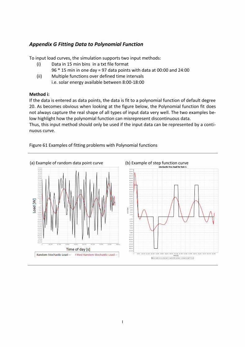
I
Appendix G Fitting Data to Polynomial Function
To input load curves, the simulation supports two input methods:
(i) Data in 15 min bins in a txt file format 96 * 15 min in one day = 97 data points with data at 00:00 and 24:00
(ii) Multiple functions over defined time intervals i.e. solar energy available between 8:00-18:00
Method i: If the data is entered as data points, the data is fit to a polynomial function of default degree 20. As becomes obvious when looking at the figure below, the Polynomial function fit does not always capture the real shape of all types of input data very well. The two examples be-low highlight how the polynomial function can misrepresent discontinuous data. Thus, this input method should only be used if the input data can be represented by a conti-nuous curve.
Figure 61 Examples of fitting problems with Polynomial functions
(a) Example of random data point curve (b) Example of step function curve
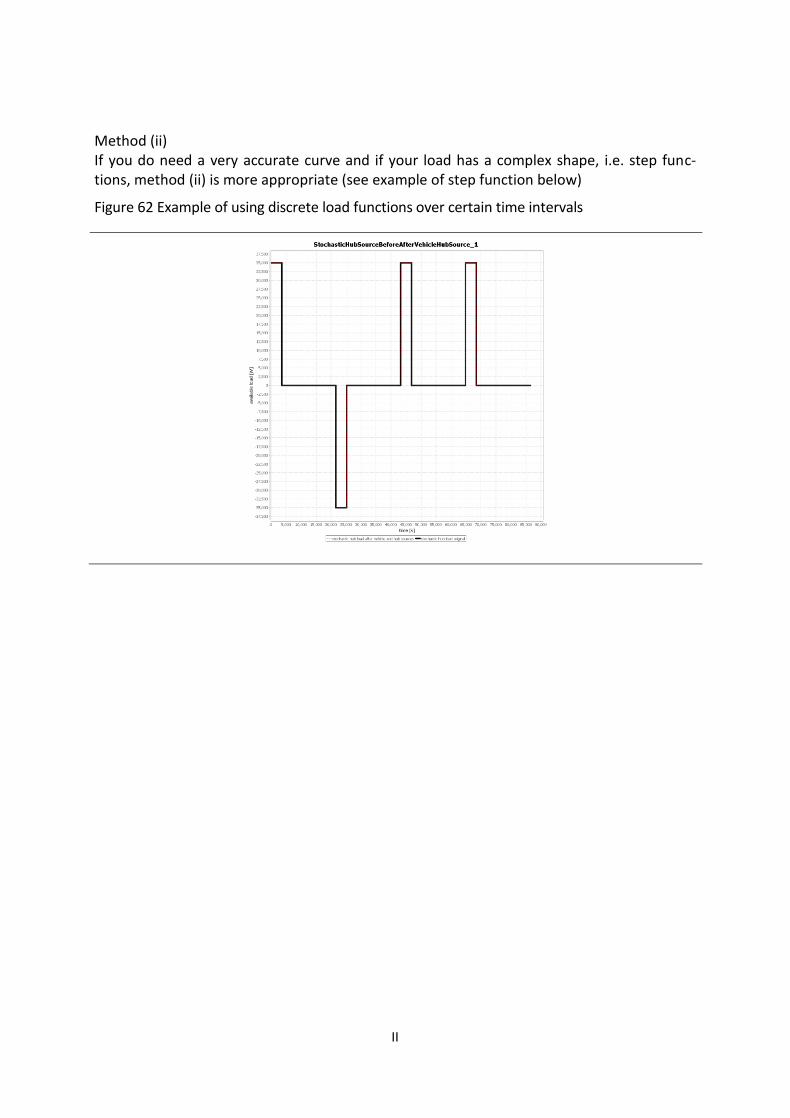
II
Method (ii) If you do need a very accurate curve and if your load has a complex shape, i.e. step func-tions, method (ii) is more appropriate (see example of step function below)
Figure 62 Example of using discrete load functions over certain time intervals
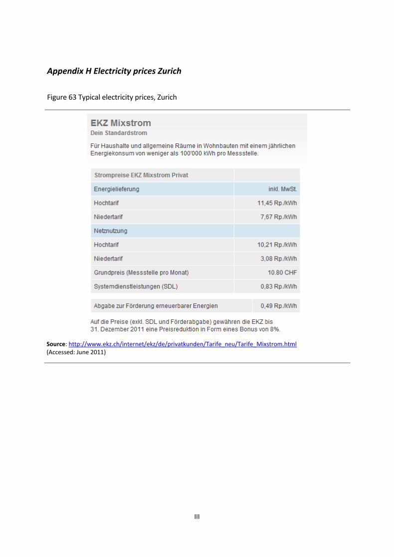
III
Appendix H Electricity prices Zurich
Figure 63 Typical electricity prices, Zurich
Source: http://www.ekz.ch/internet/ekz/de/privatkunden/Tarife_neu/Tarife_Mixstrom.html (Accessed: June 2011)
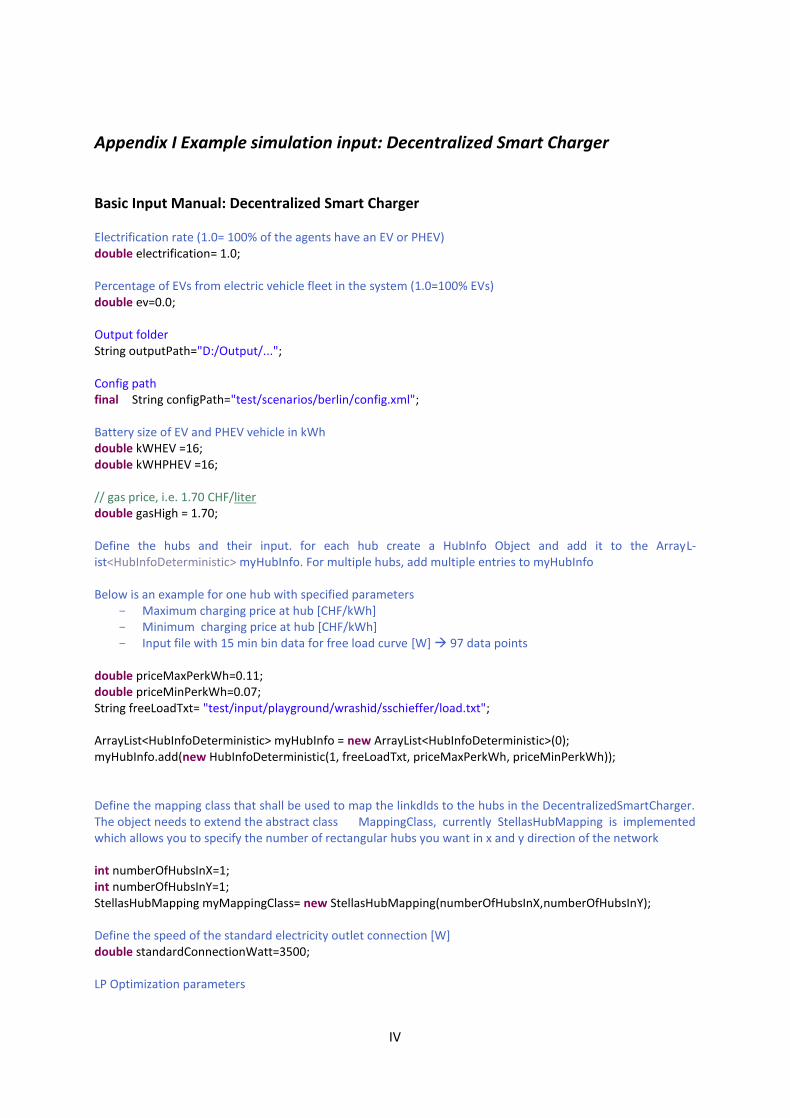
IV
Appendix I Example simulation input: Decentralized Smart Charger
Basic Input Manual: Decentralized Smart Charger Electrification rate (1.0= 100% of the agents have an EV or PHEV) double electrification= 1.0; Percentage of EVs from electric vehicle fleet in the system (1.0=100% EVs) double ev=0.0; Output folder String outputPath="D:/Output/..."; Config path final String configPath="test/scenarios/berlin/config.xml"; Battery size of EV and PHEV vehicle in kWh double kWHEV =16; double kWHPHEV =16; // gas price, i.e. 1.70 CHF/liter double gasHigh = 1.70; Define the hubs and their input. for each hub create a HubInfo Object and add it to the ArrayL-ist<HubInfoDeterministic> myHubInfo. For multiple hubs, add multiple entries to myHubInfo Below is an example for one hub with specified parameters
- Maximum charging price at hub [CHF/kWh] - Minimum charging price at hub [CHF/kWh] - Input file with 15 min bin data for free load curve [W] 97 data points
double priceMaxPerkWh=0.11; double priceMinPerkWh=0.07; String freeLoadTxt= "test/input/playground/wrashid/sschieffer/load.txt"; ArrayList<HubInfoDeterministic> myHubInfo = new ArrayList<HubInfoDeterministic>(0); myHubInfo.add(new HubInfoDeterministic(1, freeLoadTxt, priceMaxPerkWh, priceMinPerkWh)); Define the mapping class that shall be used to map the linkdIds to the hubs in the DecentralizedSmartCharger. The object needs to extend the abstract class MappingClass, currently StellasHubMapping is implemented which allows you to specify the number of rectangular hubs you want in x and y direction of the network int numberOfHubsInX=1; int numberOfHubsInY=1; StellasHubMapping myMappingClass= new StellasHubMapping(numberOfHubsInX,numberOfHubsInY); Define the speed of the standard electricity outlet connection [W] double standardConnectionWatt=3500; LP Optimization parameters
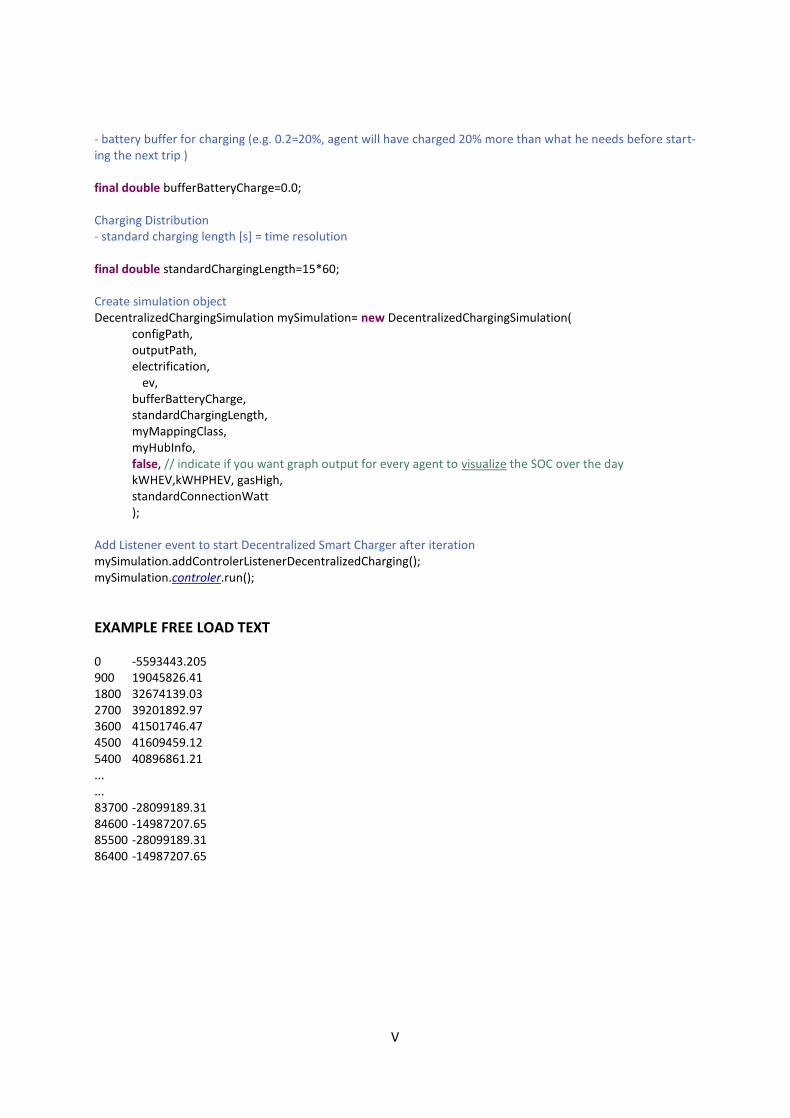
V
- battery buffer for charging (e.g. 0.2=20%, agent will have charged 20% more than what he needs before start-ing the next trip ) final double bufferBatteryCharge=0.0; Charging Distribution - standard charging length [s] = time resolution final double standardChargingLength=15*60; Create simulation object DecentralizedChargingSimulation mySimulation= new DecentralizedChargingSimulation( configPath, outputPath, electrification,
ev, bufferBatteryCharge, standardChargingLength, myMappingClass, myHubInfo, false, // indicate if you want graph output for every agent to visualize the SOC over the day kWHEV,kWHPHEV, gasHigh, standardConnectionWatt ); Add Listener event to start Decentralized Smart Charger after iteration mySimulation.addControlerListenerDecentralizedCharging(); mySimulation.controler.run();
EXAMPLE FREE LOAD TEXT 0 -5593443.205 900 19045826.41 1800 32674139.03 2700 39201892.97 3600 41501746.47 4500 41609459.12 5400 40896861.21 ... ... 83700 -28099189.31 84600 -14987207.65 85500 -28099189.31 86400 -14987207.65

VI
Appendix J Example simulation input: V2G (Additional to Input for Decentralized Smart Charger) Information about all stochastic loads at the hubs as an ArrayList<HubInfoStochastic> Object ArrayList<HubInfoStochastic> myStochasticHubInfo = new ArrayList<HubInfoStochastic>(0); GENERAL STOCHASTIC LOAD (REQUIRED) To add a general stochastic hub load at hub 1, specify the 96 bin data of the stochastic load as an input .txt. file and add it to the new HubInfoStochastic Object for hub 1 String stochasticGeneral= "stochastic.txt"; HubInfoStochastic hubInfo1= new HubInfoStochastic(1, stochasticGeneral); HUBSOURCES (OPTIONAL) To add a hub load, create a general source object and add it to the ArrayList ArrayList<GeneralSource> generalHubSource= new ArrayList<GeneralSource>(0); To define the general source with discrete load intervals, create the new General Source with an ArrayList of LoadDistribution Intervals ArrayList<LoadDistributionInterval> generalHubLoad= new ArrayList<LoadDistributionInterval>(0); generalHubLoad.add(new LoadDistributionInterval(3500, 7000, 5000)); generalHubSource.add(new GeneralSource( generalHubLoad, //ArrayList of Loads at hub source new IdImpl(1), //LinkId
"discrete load", // name 0.005) ); // compensation for feed in ArrayList<GeneralSource> generalHubSource= new ArrayList<GeneralSource>(0); To define the general source with a continuous load curve, create the new General Source with a 96 bin .txt file String hubSourceLoad= "stochasticHubLoad.txt"; generalHubSource.add(new GeneralSource( hubSourceLoad, // input .txt file new IdImpl(2), "continuous load", 0.005)); Add all hub loads to hubInfo hubInfo1.setStochasticGeneralSources(generalHubSource); STOCHASTIC VEHICLE LOAD (OPTIONAL) For every vehicle specify the input load intervals for every vehicle as an ArrayList of LoadDistribution intervals and save them to a HashMap with the Agent Id as an identifier. HashMap <Id, ArrayList<LoadDistributionInterval>> vehicleLoadHashMap = new HashMap<Id, ArrayL-ist<LoadDistributionInterval>>(); ArrayList<LoadDistributionInterval> vehicleLoad= new ArrayList<LoadDistributionInterval>(0); vehicleLoad.add(new LoadDistributionInterval(3500, 7000, 3500)); vehicleLoadHashMap.put(new IdImpl(1), vehicleLoad);
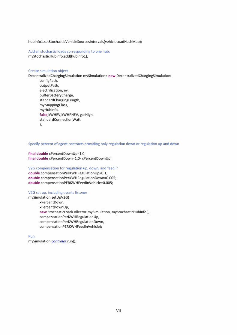
VII
hubInfo1.setStochasticVehicleSourcesIntervals(vehicleLoadHashMap); Add all stochastic loads corresponding to one hub: myStochasticHubInfo.add(hubInfo1); Create simulation object DecentralizedChargingSimulation mySimulation= new DecentralizedChargingSimulation( configPath, outputPath, electrification, ev, bufferBatteryCharge, standardChargingLength, myMappingClass, myHubInfo, false,kWHEV,kWHPHEV, gasHigh, standardConnectionWatt ); Specify percent of agent contracts providing only regulation down or regulation up and down final double xPercentDownUp=1.0; final double xPercentDown=1.0- xPercentDownUp; V2G compensation for regulation up, down, and feed in double compensationPerKWHRegulationUp=0.1; double compensationPerKWHRegulationDown=0.005; double compensationPERKWHFeedInVehicle=0.005; V2G set up, including events listener mySimulation.setUpV2G( xPercentDown, xPercentDownUp, new StochasticLoadCollector(mySimulation, myStochasticHubInfo ), compensationPerKWHRegulationUp, compensationPerKWHRegulationDown, compensationPERKWHFeedInVehicle); Run mySimulation.controler.run();
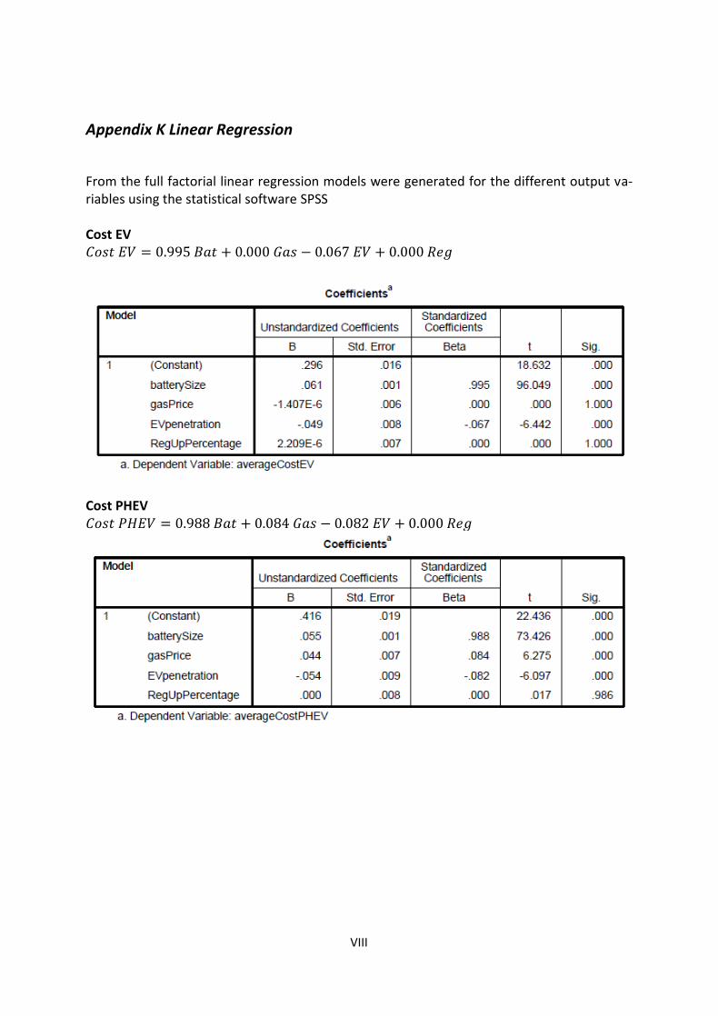
VIII
Appendix K Linear Regression
From the full factorial linear regression models were generated for the different output va-riables using the statistical software SPSS Cost EV
Cost PHEV
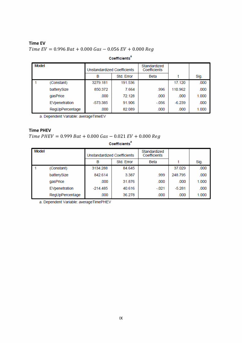
IX
Time EV
Time PHEV
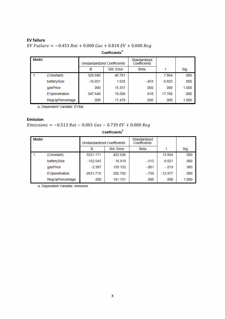
X
EV failure
Emission
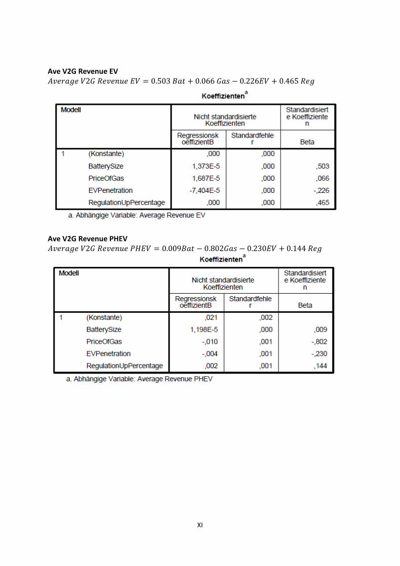
XI
Ave V2G Revenue EV
Ave V2G Revenue PHEV
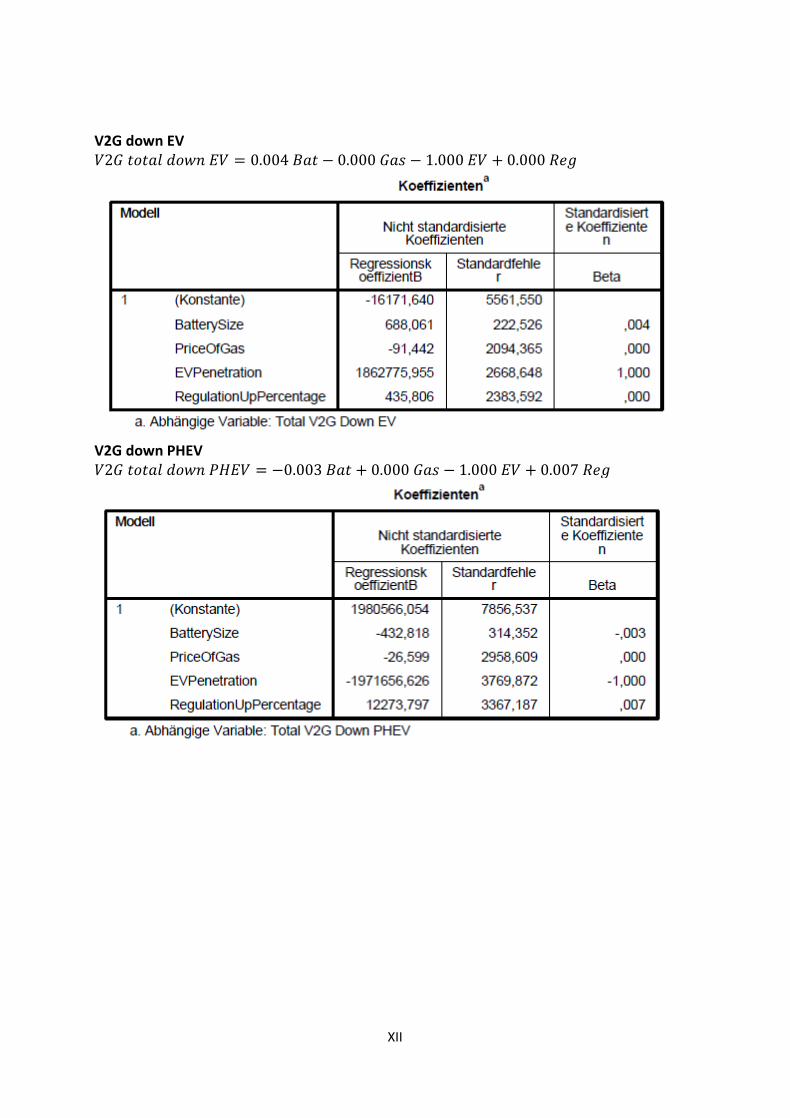
XII
V2G down EV
V2G down PHEV
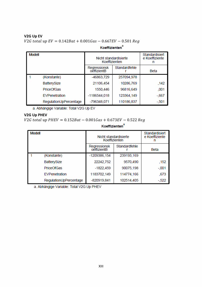
XIII
V2G Up EV
V2G Up PHEV
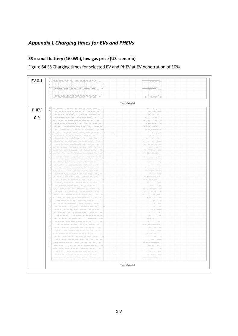
XIV
Appendix L Charging times for EVs and PHEVs
SS = small battery (16kWh), low gas price (US scenario)
Figure 64 SS Charging times for selected EV and PHEV at EV penetration of 10%
EV 0.1
Time of day [s]
PHEV
0.9
Time of day [s]
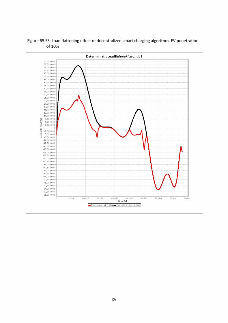
XV
Figure 65 SS: Load flattening effect of decentralized smart charging algorithm, EV penetration of 10%
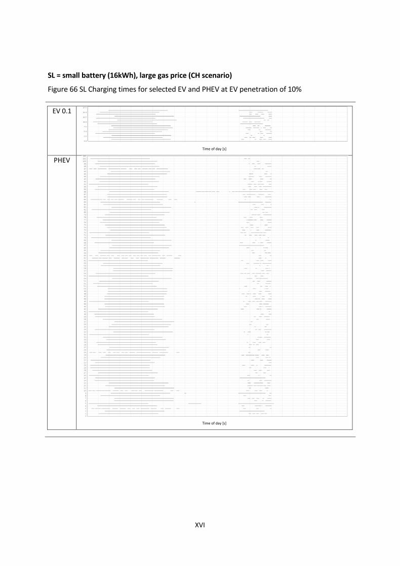
XVI
SL = small battery (16kWh), large gas price (CH scenario)
Figure 66 SL Charging times for selected EV and PHEV at EV penetration of 10%
EV 0.1
Time of day [s]
PHEV
Time of day [s]
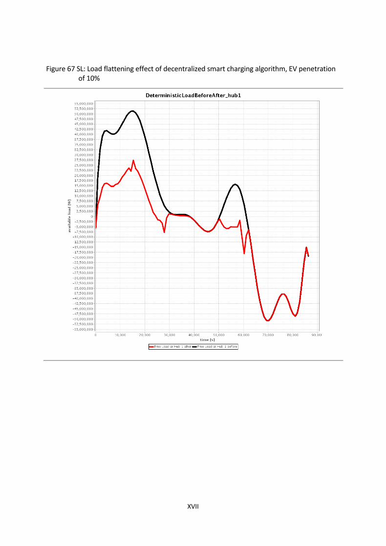
XVII
Figure 67 SL: Load flattening effect of decentralized smart charging algorithm, EV penetration of 10%

XVIII
LS = large battery (24kWh), small gas price (CH scenario)
Figure 68 LS Charging times for selected EV and PHEV at EV penetration of 10%
EV
Time of day [s]
PHEV
Time of day [s]
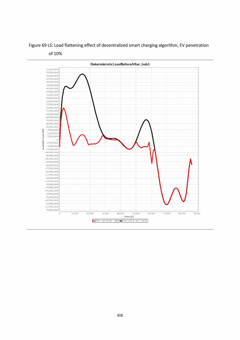
XIX
Figure 69 LS: Load flattening effect of decentralized smart charging algorithm, EV penetration
of 10%