1

Decentralized Adaptive Control forCollaborative Manipulation of Rigid Bodies

Preston Culbertson, Jean-Jacques E. Slotine, and Mac Schwager

Abstract—In this work, we consider a group of robotsworking together to manipulate a rigid object to track adesired trajectory in SE(3). The robots have no explicitcommunication network among them, and they do notknow the mass or friction properties of the object, or wherethey are attached to the object. However we assume theyshare data from a common IMU placed arbitrarily on theobject. To solve this problem, we propose a decentralizedadaptive control scheme wherein each agent maintains andadapts its own estimate of the object parameters in orderto track a reference trajectory. We present an analysis ofthe controller’s behavior, and show that all closed-loopsignals remain bounded, and that the system trajectorywill almost always (except for initial conditions on a set ofmeasure zero) converge to the desired trajectory. We studythe proposed controller’s performance using numericalsimulations of a manipulation task in 3D, as well ashardware experiments which demonstrate our algorithm ona planar manipulation task. These studies, taken together,demonstrate the effectiveness of the proposed controllereven in the presence of numerous unmodeled effects, suchas discretization errors and complex frictional interactions.

I. INTRODUCTION

As robots are fielded in applications ranging fromdisaster relief to autonomous construction, it is likely thatsuch applications will, at times, require manipulation ofobjects which exceed a single robot’s actuation capacities(e.g. debris removal, material transport) [1]. Notably,when humans undertake such tasks, they are able to worktogether to flexibly and reliably transport objects whichare too massive for one person alone. We are interestedin enabling similar capabilities in robot teams.

In this work, we consider the problem of cooperativemanipulation, where a group of robots works togetherto manipulate a common payload. This problem haslong been of significant interest to both the multi-robotsystems community, and the broader robotics community[2], since it requires close collaboration between robotsin addition to the numerous sensing and actuation chal-lenges involved in any manipulation task.

While collaborative manipulation has been studiedin literature [3]–[5], manipulation teams are still quitelimited in their functionality. In part, this is due to theirreliance on extensive prior information about the payloadto be manipulated, and their need for high-bandwidth,two-way communication either with other agents or a

centralized planner. The requirement of exact payloadknowledge (i.e. the payload’s mass, inertial properties,and the location of its center of mass) imposes therequirement that every payload be thoroughly calibratedprior to manipulation, in addition to making manipula-tion teams brittle in the face of parameter uncertainty.Further, the utilization of communication networks in-troduces not only an additional point of failure, but alsolatency, which can limit the team’s speed and robustness.

In this work, we take a minimalist approach to collab-orative manipulation, and present an adaptive controllerfor collaborative manipulation that requires neither priorpayload characterization nor point-to-point communica-tion between agents. To achieve this, we use an SE(3)sliding model control architecture, together with a decen-tralized adaptation law, which allows the manipulationteam to adapt to unknown payload dynamics withoutexplicit communication; we also prove our controller’sconvergence to tracking a reference trajectory usingBarbalat’s lemma. We only require that the agents ob-tain information from a common IMU sensor locatedsomewhere on the body, or on one of the manipulationrobots. This IMU could be wired to all the robots, or maybroadcast its measurements to all robots over a simpleone-way broadcast network.

Intuitively, during manipulation each agent executesthe proposed controller, with its individual set of pa-rameters (or, equivalently, control gains). The agentsthen use measurements from the common IMU to adapttheir local parameters, such that the location of theIMU asymptotically tracks a desired trajectory. Such anapproach leads to a manipulation algorithm which caneasily scale in the number of agents, and is flexibleenough to manipulate a large variety of payloads, whiletolerating both parameter uncertainty and single-agentfailure.

This paper proposes control and adaptation lawsfor manipulation tasks in both the plane and three-dimensional space, in addition to a proof of convergenceto the desired trajectory, as well as the boundedness of allclosed-loop signals. We further validate the controller’sperformance both numerically, simulating a manipulationtask in 3D, and experimentally, using a team of groundrobots performing a planar manipulation task.

2

II. PRIOR WORK

Collaborative manipulation has been a subject of bothsustained and broad interest in multi-robot systems.Early work such as [6] first proposed multi-arm ma-nipulation strategies which used a central computer tocontrol each arm. This early work was followed with aflurry of interest, including [3], [7], where the authorsstudy the dynamics and force allocation of redundantmanipulators, and [8], which investigates various controlstrategies for multiple arms. A number of authors [9]–[11] have used impedance controllers for collaborativemanipulation, in order to yield compliant object behav-ior, as well as to avoid large internal forces on thepayload. An approach for characterizing such forces isproposed in [12].

While early work focused almost exclusively on multi-arm manipulation, often with centralized architecturesand only a few robots, other authors have focusedinstead on collaborative manipulation with large teamsof mobile robots. In [5] and [13], the authors movefurniture with small mobile robots, with a focus onreducing the communication and sensing requirementsof manipulation algorithms. Other works have studiedvarious decentralized manipulation strategies, includingpotential fields [14], caging [4], and distributed controlallocation via matrix pseduo-inverse [15].

The problem of collaborative manipulation with aerialvehicles (such as quadrotors) has received extensive re-cent interest. In [16], the authors consider the problem ofcollaborative lifting using quadrotors which rigidly graspa common payload; they use a least-squares solutionto allocate control efforts between agents. Further, theproblem of aerial towing (manipulation via cables) hasbeen studied in works such as [17]–[19]. The authors in[20] use a distributed optimization algorithm to performcollaborative manipulation of a cable-suspended load.

While collaborative manipulation has been studied ina variety of settings, most work often relies on restrictiveassumptions, such as communication between agents orprior knowledge of the object parameters, which limitthe practical applicability of their approaches. Morerecent work has focused on removing these assump-tions. In [21], the authors propose a controller whichallows a group of agents to reach a force consensuswithout communication, using only the payload dy-namics; a leader can steer this consensus to have theobject track a desired trajectory. Further, [22] proposesa communication-free controller for collaborative ma-nipulation with aerial robots, using online optimizationto allocate control effort. Other works, such as [23],[24] propose distributed schemes for estimating objectparameters, and using these estimates for control, usingcommunication between agents to reach consensus onestimated parameters.

Previous work has proposed applying adaptive controlto collaborative manipulation. The authors of [25] pro-pose a centralized adaptive control scheme, which theydemonstrate experimentally with a pair of robot arms.In [26], the authors propose a centralized robust adaptivecontroller for a group of mobile manipulators performinga collaborative manipulation task.

Perhaps closest to this work is [27], [28], whichalso propose distributed adaptive control schemes forcollaborative manipulation. This work differs from pre-vious literature in adapting both inertial and geometricparameters of the body; previous methods require exactmeasurement of manipulators’ relative positions fromthe center of mass in order to invert the grasp matrix[29], which relates wrenches applied at contact pointsto wrenches applied at the center of mass. We arguethat this assumption is quite restrictive, since, in practice,this amounts to knowing exactly how the body’s trans-lational and rotational dynamics are coupled. Accuratelylocalizing large numbers of manipulators (especiallywith respect to the center of mass) can be both timeconsuming and difficult; it is also unclear why the body’snormalized first moment of mass (i.e. the center ofmass) is assumed known, while its zeroth (mass) andsecond moments (inertia tensor) are assumed unknown.In contrast, our method can treat a much broader classof model parameters (including inertial, geometric, andother effects such as gravity and friction) as unknowns,and handle them through online adaptation. We believethat this provides greater robustness to uncertainty inthese parameters, and eliminates the need to estimatethese quantities before manipulation.

An early version of this work appeared in [30]; thiswork differs greatly from the original version. The mostfundamental difference is that this work builds on theSlotine-Li adaptive controller [31], which allows formuch more efficient parameterization than the generalmodel reference adaptive controller in the original ver-sion. We do not constrain the measurement point to lie atthe center of mass, and further introduce a sliding vari-able that allows for trajectory tracking instead of simplevelocity control. Finally, we present new simulation andexperimental results studying the novel controller.

Our basic algorithm can also be compared to quorumsensing [32], [33], a natural phenomenon in whichorganisms or cells can exchange information [34] andsynchronize themselves using a noisy, shared environ-ment, instead of using direct information exchange. Suchmechanisms have been shown to reduce the influenceof random noise on synchronization phenomena [32],allowing for meaningful coordination without central-ized control or explicit communication. The proposedalgorithm can be seen as analogous to quorum sensing,wherein the common object acts as the shared envi-

3

ronment, which allows the agents to coordinate theircontrol actions to achieve tracking without using directcommunication.

III. PROBLEM STATEMENT

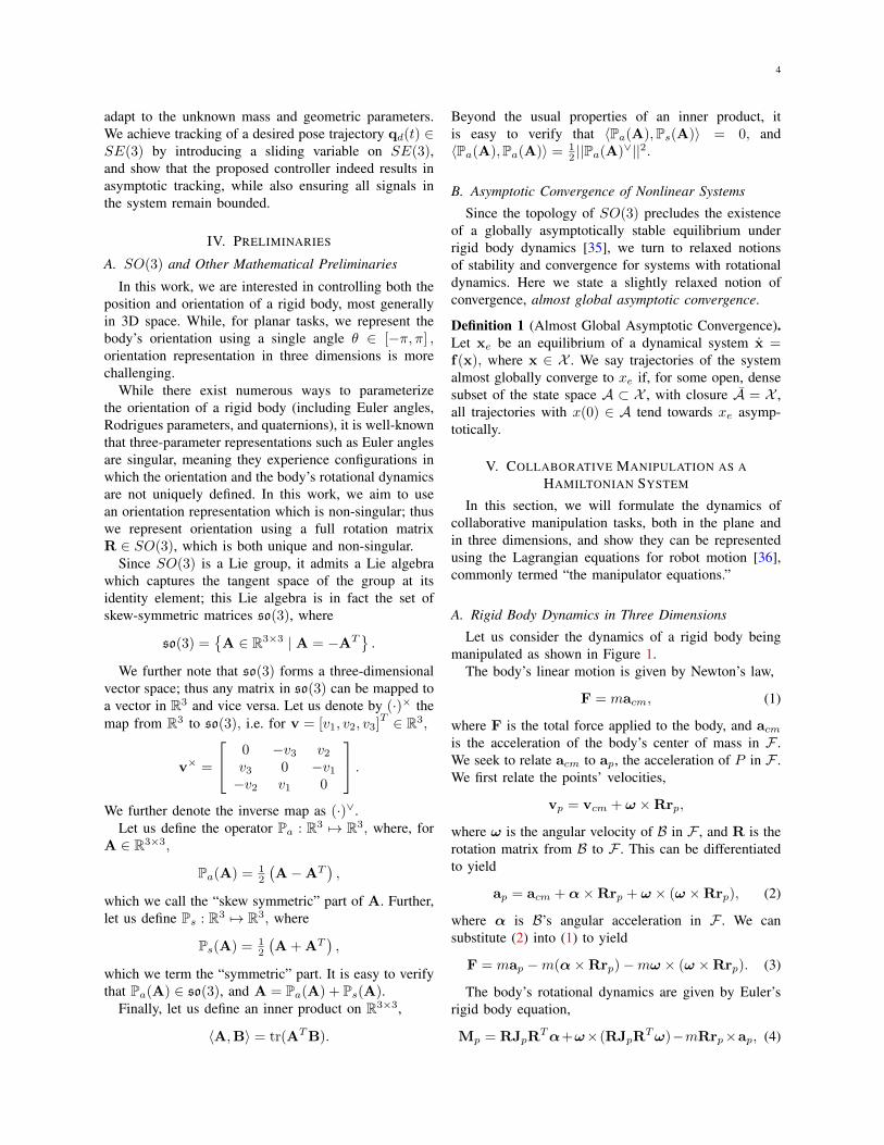
We consider a rigid body which undergoes generalmotion (i.e. translation and rotation), during collabora-tive manipulation by a team of N autonomous agents.There exists a world-fixed (Newtonian) frame F , as wellas a body-fixed frame B, which is centered at bcm, thebody’s center of mass. There also exists P , a generalpoint fixed to the body, which is located at rp in B. Thebody has mass m and body-frame inertia of Icm aboutits center of mass. Figure 1 shows a schematic of thesystem.

Fig. 1. Schematic of Collaborative Manipulation Task

Each agent is rigidly attached to the body at ri fromP , and applies a wrench τi, i.e. a combined force andtorque. We assume the agents are attached rigidly tothe object, and can apply a full wrench (both force andtorque) at their attachment point.

We describe the body’s pose in F using a configura-tion variable q = (x,R) ∈ Rn × SO(n), where

SO(n) ={R ∈ Rn×n | RTR = I,det(R) = 1

},

is the group of rotation matrices, x is the position of thereference point P in F , R is the body-to-world rotationmatrix relating B and F , and n ∈ {2, 3}, depending onif the manipulation task is in the plane or in general 3Dspace, respectively. For simplicity, we say

Rn × SO(n) ∼= SE(n),

i.e. we denote this set as the Special Euclidean group,

SE(n) =

{[R v0 1

]| R ∈ SO(n),v ∈ Rn

}which is the set of (n + 1) × (n + 1) transformationmatrices, since these spaces are homeomorphic. Abusingnotation, we define q =

[xT ,ωT

]T ∈ R3n−3 whichappends x, the velocity of P in F , with ω, the body’sangular rate(s) in F .

We now define the control problem considered in thiswork.

Problem 1. Assume each agent can measure the body’spose q and rates q, but has no knowledge of its massproperties (m, Icm) or geometry (rp, ri), and cannotexplicitly communicate with other agents. Design acontrol law for each agent which allows the body to tracka desired trajectory qd(t) ∈ SE(n) asymptotically.

It is apparent that solving Problem 1 achieves col-laborative manipulation under few assumptions on theinformation available to each agent, and their ability tocommunicate. However, the assumption of a commonmeasurement (q, q) warrants additional motivation.

At a high level, we aim to collaboratively controlboth the linear and rotational dynamics of the object;but in defining a reference trajectory qd(t) ∈ SE(n),we must additionally define which point on the body wewish to track this trajectory. Since we assume the body’sgeometry is unknown, even if the agents can measuretheir own states, they have no way of computing orestimating the state of the measurement point; thus thecontrol problem is ill-posed.

In this work, since we aim to track general trajectorieson SE(n), we allow the agents to simply measure thepose of the reference point; this can be achieved inpractice by placing a sensor anywhere on the body, orby having a single agent broadcast its measurements tothe other agents. We note this broadcast communicationarchitecture is much simpler than a point-to-point or“mesh” network.

However, different assumptions can be made if westill wish to solve Problem 1, but without the use ofa common measurement. One option is to restrict theclass of desired trajectories qd; if the body’s angularvelocity ω = 0, then the velocity is uniform across allpoints on the body, and robots can use their own velocitymeasurements xi in order to track a desired linear veloc-ity xd. Similarly, if we only seek to control the body’sorientation R, if the agents share a reference frame,then their pose measurements are identical, making theproblem again well-posed.

Finally, we can eliminate the need for a common mea-surement if we assume the agents know their position riwith respect to the measurement point, as in [27], [28].Using this information, the agents can easily computethe position and velocity of the reference point fromtheir own measurements. However, we argue such anassumption is quite restrictive, since each agent mustnow have some way of localizing itself on the bodybefore starting a manipulation task. We further note thatsuch a method is not robust to errors in measuring ri,which could introduce unmodeled sources of uncertainty.

To solve Problem 1, we propose a modified formof the Slotine-Li adaptive manipulator controller [31],which is generalized to the multi-agent case, and can

4

adapt to the unknown mass and geometric parameters.We achieve tracking of a desired pose trajectory qd(t) ∈SE(3) by introducing a sliding variable on SE(3),and show that the proposed controller indeed results inasymptotic tracking, while also ensuring all signals inthe system remain bounded.

IV. PRELIMINARIES

A. SO(3) and Other Mathematical Preliminaries

In this work, we are interested in controlling both theposition and orientation of a rigid body, most generallyin 3D space. While, for planar tasks, we represent thebody’s orientation using a single angle θ ∈ [−π, π] ,orientation representation in three dimensions is morechallenging.

While there exist numerous ways to parameterizethe orientation of a rigid body (including Euler angles,Rodrigues parameters, and quaternions), it is well-knownthat three-parameter representations such as Euler anglesare singular, meaning they experience configurations inwhich the orientation and the body’s rotational dynamicsare not uniquely defined. In this work, we aim to usean orientation representation which is non-singular; thuswe represent orientation using a full rotation matrixR ∈ SO(3), which is both unique and non-singular.

Since SO(3) is a Lie group, it admits a Lie algebrawhich captures the tangent space of the group at itsidentity element; this Lie algebra is in fact the set ofskew-symmetric matrices so(3), where

so(3) ={A ∈ R3×3 | A = −AT

}.

We further note that so(3) forms a three-dimensionalvector space; thus any matrix in so(3) can be mapped toa vector in R3 and vice versa. Let us denote by (·)× themap from R3 to so(3), i.e. for v = [v1, v2, v3]

T ∈ R3,

v× =

0 −v3 v2v3 0 −v1−v2 v1 0

.We further denote the inverse map as (·)∨.

Let us define the operator Pa : R3 7→ R3, where, forA ∈ R3×3,

Pa(A) = 12

(A−AT

),

which we call the “skew symmetric” part of A. Further,let us define Ps : R3 7→ R3, where

Ps(A) = 12

(A + AT

),

which we term the “symmetric” part. It is easy to verifythat Pa(A) ∈ so(3), and A = Pa(A) + Ps(A).

Finally, let us define an inner product on R3×3,

〈A,B〉 = tr(ATB).

Beyond the usual properties of an inner product, itis easy to verify that 〈Pa(A),Ps(A)〉 = 0, and〈Pa(A),Pa(A)〉 = 1

2 ||Pa(A)∨||2.

B. Asymptotic Convergence of Nonlinear Systems

Since the topology of SO(3) precludes the existenceof a globally asymptotically stable equilibrium underrigid body dynamics [35], we turn to relaxed notionsof stability and convergence for systems with rotationaldynamics. Here we state a slightly relaxed notion ofconvergence, almost global asymptotic convergence.

Definition 1 (Almost Global Asymptotic Convergence).Let xe be an equilibrium of a dynamical system x =f(x), where x ∈ X . We say trajectories of the systemalmost globally converge to xe if, for some open, densesubset of the state space A ⊂ X , with closure A = X ,all trajectories with x(0) ∈ A tend towards xe asymp-totically.

V. COLLABORATIVE MANIPULATION AS AHAMILTONIAN SYSTEM

In this section, we will formulate the dynamics ofcollaborative manipulation tasks, both in the plane andin three dimensions, and show they can be representedusing the Lagrangian equations for robot motion [36],commonly termed “the manipulator equations.”

A. Rigid Body Dynamics in Three Dimensions

Let us consider the dynamics of a rigid body beingmanipulated as shown in Figure 1.

The body’s linear motion is given by Newton’s law,

F = macm, (1)

where F is the total force applied to the body, and acmis the acceleration of the body’s center of mass in F .We seek to relate acm to ap, the acceleration of P in F .We first relate the points’ velocities,

vp = vcm + ω ×Rrp,

where ω is the angular velocity of B in F , and R is therotation matrix from B to F . This can be differentiatedto yield

ap = acm +α×Rrp + ω × (ω ×Rrp), (2)

where α is B’s angular acceleration in F . We cansubstitute (2) into (1) to yield

F = map −m(α×Rrp)−mω × (ω ×Rrp). (3)

The body’s rotational dynamics are given by Euler’srigid body equation,

Mp = RJpRTα+ω×(RJpR

Tω)−mRrp×ap, (4)

5

where Jp is the body’s inertia matrix about bp, whichis given by

Jp = Jcm +m((rTp rp)I− rpr

Tp

),

where I denotes the identity matrix.We again define the configuration variable q =

[x,R] ∈ R3 × SO(3), where x is the position of themeasurement point in F . Abusing notation, we can letq, q ∈ R6, where q =

[xT ,ωT

]Trepresents the body’s

linear and angular rates, and q =[xT ,αT

]Trepresents

its linear and angular accelerations.Using these configuration variables, we can now write

(2) and (4) more compactly as

τ = H(q)q + C(q, q)q, (5)

where τ is the total wrench applied to the body aboutthe measurement point, where

H(q) =

[mI m(Rrp)

×

−m(Rrp)× RJpR

T

]is the system’s inertia matrix (which is symmetric,positive definite), and

C(q, q) =

[03 mω×(Rrp)

×

−mω×(Rrp)× ω×RIpR

T −m((Rrp)×x)×

]is a matrix which contains centrifugal and Coriolis terms,with the 3× 3 zero matrix denoted by 03.

Further, we can show that these matrices have anumber of interesting properties. Specifically, H(q) ispositive definite for all q, and H − 2C is skew-symmetric. These properties can be viewed as matrixversions of common properties of Hamiltonian systems(e.g. conservation of energy). Proof of these propertiesis included in Appendix A.

B. Grasp Matrix and its Properties

While the dynamics in (5) describe the body’s motionunder the total wrench τ about bp, we must furtherexpress τ as a function of each robot’s applied wrenchτi. We can write τ as

τ =

N∑i=1

M(q, ri)τi,

where M denotes the grasp matrix, which is given by

M(q, ri) =

[I 03

(Rri)× I

],

where agent i grasps the object at some point ri fromthe measurement point. We denote the set of such graspmatrices as M.

The grasp matrix has some unique properties, specif-ically,

M(ri)−1 =

[I 03

−(Rri)× I

]= M(−ri),

and

M(ri)M(rj) =

[I 03

(R(ri + rj))×

I

]= M(ri) + M(rj)− I. (6)

Thus, interestingly, for two matrices inM, their productis simply equal to their sum, minus the identity.

C. Rigid Body Dynamics for Planar Tasks

We now turn to the case of SE(2), when a group ofagents seeks to manipulate a rigid body in the plane.Thus, we constrain the translational dynamics of thebody in the z-dimension, and its rotational dynamics inthe x- and y-dimensions to be fixed.

Accordingly, the dynamics of the planar task mayalso be described by (5), but with q ∈ R2 × SO(2),q, q ∈ R3, due to the reduced degrees of freedom. Thus,enforcing the planar constraints yields

H(q) =

m 0 mrNy0 m −mrNx

mrNy −mrNx Jp

,and

C(q, q) =

0 0 mrNx ω0 0 mrNy ω0 0 0

,where rNp =

[rNx , r

Ny , 0

]T= R(θ)rBp , is the location

of the measurement point in the global frame F , θis an angle which expresses the body’s orientation inthe global frame, ω is the body’s angular velocity, andR(θ) ∈ SO(2) is the body-to-world rotation matrix, with

R(θ) =

cos(θ) sin(θ) 0− sin(θ) cos(θ) 0

0 0 1

.Further, when computing the total wrench τ applied

to the body, we include a frictional force Ff,i which isapplied at the contact point of each robot. Thus, we canexpress the total wrench as

τ =

N∑i=1

M(q, ri) (τi − Ff,i) ,

where τi is the wrench applied by agent i, and

M(q, ri) =

1 0 00 1 0−rNi,y rNi,x 1

is the grasp matrix for agent i, where rNi =[rNi,x, r

Ni,y0]T

= R(θ)rBi is the agent’s attachment pointexpressed in the global frame. Thus, the full planardynamics are given by

H(q)q + C(q, q)q =

N∑i=1

Mi(q) (τi − Ff,i) ,

6

where we omit the dependence of Mi on ri for clarity.It is clear by inspection that these dynamics are of thesame class as those in three dimensions (5).

Importantly, although the dynamics evolve in a lower-dimensional space, all properties from the full three-dimensional case hold, including the positive definitenessof H, skew-symmetry of H − 2C, and grasp matrixproperties of Mi.

VI. DECENTRALIZED ADAPTIVE TRAJECTORYTRACKING

We will now propose a decentralized adaptive con-troller suitable for accomplishing the collaborative ma-nipulation tasks outlined previously, and provide proofsof boundedness of signals, and almost global asymptotictracking.

A. Proposed Sliding Variable on SE(3)× R6

We begin by proposing a sliding surface for 3D posesand their derivatives, which lie in SE(3)×R6. Adaptivecontrollers for Hamiltonian manipulators in literature(cf. [37, Chapter 9]) typically utilize sliding surfaceswhich correspond to a linear subspace, and thus havelinear error dynamics on the surface. Such a surface isappropriate for configuration variables (such as positionsand small joint angles) which lie in Cartesian space.

However, since we aim to track both a desired po-sition xd and orientation Rd, the system’s dynamicsdo not evolve naturally in Cartesian space. We thuspropose a sliding variable s which is non-singular,inherits the topology of SE(3), and exhibits almostglobal convergence when on the sliding surface D ={

(qe, qe) ∈ SE(3)× R6 | s(qe, qe) = 0}

. To achievethis, we borrow the sliding variable on SO(3) from [38],and combine it with a typical linear sliding variable onR3 to define a sliding surface on SE(3). We then use aLyapunov-like proof to show almost global convergenceto tracking of the desired orientation trajectory when onthe surface.

We aim to control the body to track a desired positionxd(t), and a desired orientation, Rd, which satsifies

Rd = ω×d Rd,

for some desired angular velocity ωd. Let us define therotational and angular velocity errors as Re = RT

d R,and ωe = ω − ωd, noting

(Re,ωe) = (I,0) ⇐⇒ (R,ω) = (Rd,ωd).

We can further obtain the rotation error dynamics bytaking a time derivative of Re, yielding

Re = RTd R + RT

d R,

= RTd (ω − ωd)×R,

=(RTd (ω − ωd)

)×RTd R,

=(RTdωe

)×Re. (7)

Finally, we propose a sliding variable s : SE(3) ×R6 7→ R6, which is given by

s =

[s`σ

]=

[˙x + λx

ωe + λRdPa(Re)∨

],

where x = x − xd is the linear tracking error, and s` :R3 × R3 7→ R3 and σ : SO(3) × R3 7→ R3 are slidingvariables for the object’s linear and angular dynamics,respectively.

B. System Behavior on Sliding SurfaceWe now consider the system’s behavior when it lies

on the sliding surface s = 0. The behavior of the lineardynamics is obvious; imposing the condition s` = 0results in the linear error dynamics

˙x = −λx,

which defines a stable linear system. Thus, once onthe sliding surface, the position tracking error x tendsexponentially to zero, with time constant 1

λ .Thus, we turn our attention to the rotational error

dynamics which are defined by σ = 0. Imposing thiscondition results in the rotational dynamics

Re =(−λRT

d RdPa(Re)∨)×Re,

= −λPa(Re)Re,

using the rotation error dynamics given by (7). We notethat (Re,ωe) = (I,0) both lies on the sliding surface,and is an equilibrium of the reduced-order rotationaldynamics.

Theorem 1. The rotation error (Re,ωe) almost globallyconverges to the equilibrium (I,0) for the reduced-ordersystem given by σ = 0.

Proof. Consider the Lyapunov function candidate

VR(t) = tr (I−Re) > 0,

which is positive definite since −1 ≤ tr(Re) ≤ 3 forall Re ∈ SO(3), with tr(Re) = 3 iff Re = I. The timederivative of VR is given by

VR = − tr(Re),

= λ tr(Pa(Re)Re),

= λ 〈−Pa(Re),Re〉 ,= −λ 〈Pa(Re),Pa(Re) + Ps(Re)〉 ,= −λ2 ||Pa(Re)

∨||2 ≤ 0,

7

using the matrix inner product 〈A,B〉 = tr(ATB), andthe fact that 〈Pa(A),Ps(A)〉 = 0, for A,B ∈ R3×3.

Further, invoking Barbalat’s lemma, [37, Chapter 4.5],we can conclude that if VR has a finite limit, and if VR isuniformly continuous, the rotational error will convergeto the set

E ={

Re | VR = 0}.

Since VR is lower bounded, and VR is negative semi-definite, it must have a finite limit. Thus, we show VRis uniformly continuous.

To show VR is uniformly continuous, it is sufficientto show VR is bounded. To this end, we can differentiateVR to yield

VR = −λ⟨Pa(Re),Pa(Re)

⟩=λ2

2〈Pa(Re),Pa(ReRe)〉 ,

=λ2

2tr(Re −R3

e + RTe − (RT

e )3),

which must be bounded, since all matrices inside thetrace lie in SO(3), and must have a trace in [−1, 3].Thus, we must have VR uniformly continuous, whichimplies Re → E .

Again using the results from [38], we find that

E = {I} ∪{I + 2η×η× | ||η|| = 1

}.

Further, since the spurious points in E correspond tomaxima of VR, all points in E are unstable except forRe = I. Thus, since the spurious equilibria are unstable,and lie in a nowhere dense set, we conclude (Re,ωe)almost globally converges to (I,0).

Thus, we can conclude that when the system lies onthe sliding surface s = 0, it will almost globally convergeto tracking the desired position xd and orientation Rd.

We further note that s can be interpreted as a “velocityerror,” since we can write

s = q− qr,

where qr is a “reference velocity” which augments thedesired velocity qd with an additional term based on thepose error,

qr =

[xd − λx

ωd − λRdPa(Re)∨

].

C. Decentralized Adaptive Trajectory Control

We now consider the problem of decentralized adap-tive control of a common payload. We consider La-grangian dynamics of the form

H(q)q + C(q, q) + g =

N∑i=1

Mi(q)τi, (8)

which, as shown previously, hold for collaborative ma-nipulation tasks on both SE(2) and SE(3). We note thatwhile neither of the studied systems includes the termg, which models conservative forces such as gravity, weinclude it here for completeness, and to conform to thetraditional “manipulator equation.”

We now consider a Lyapunov function candidate ofthe form

V (t) = 12

[sTHs +

∑Ni=1 oTi Γ−1o oi + rTi Γ−1r ri

], (9)

where oi = oi − oi is a parameter estimation error foragent i, with oi being a vector of physical constants thatdefine the payload’s dynamics, and oi being agent i’sestimate of these parameters. Similarly, we let ri be thedifference between the vector ri from the measurementpoint to agent i, and the agent’s estimate ri. We fur-ther let Γo and Γr be positive definite matrices whichcorrespond to adaptation gains.

Differentiating V yields

V (t) = sTHs + 12sT Hs +

∑Ni=1 oTi Γ−1o

˙o + rTi Γ−1r˙ri,

using the fact that the parameter error derivatives ˙oi, ˙riare equal to the parameter estimate derivatives ˙oi, ˙ri,since the true parameter values are constant.

Further, since we can write s = q−qr, we can expandthe term

sTHs = sTH(q− qr),

= sT(∑N

i=1 Miτi −Cq− g −Hqr

),

= sT(∑N

i=1 Miτi −Hqr −Cqr − g −Cs),

using the system dynamics (8) to substitute for Hq, andthe fact that q = s + qr.

Further, since the system is over-actuated, meaning ithas many more control inputs than degrees of freedom,there exist many sets of control inputs which producethe same object dynamics. Thus, it is sufficient for eachagent to take some portion of the control effort, which,combined, enables tracking of the desired trajectory. Tothis end, let us consider a set of N positive constantsαi, with

∑Ni=1 αi = 1. If we again consider the analogy

between our proposed controller and quorum sensing[33], we can interpret these constants as akin to couplingweights between the agents.

Using these constants, we can allocate the total con-trol effort needed for feedback linearization among theagents, writing

Miτi = αi (Hq + Cq + g)

for each i. It is important to note that these constants, ineffect, only scale the physical parameters of the system,meaning they can be adapted to and do not need to beknown a priori.

8

We can also exploit an important property of thissystem, linear parameterizability. Importantly, for thecontrol tasks considered in this work, the physical pa-rameters to be estimated appear only linearly in thedynamics. Thus, we can define a known regressor matrixYo(q, q, qr, qr), such that

αi (H(q)qr + C(q, q)qr + G) = Yo(q, q, qr, qr)oi.

We further note that∑Ni=1 Yooi =

∑Ni=1 αi (Hqr + Cqr + g)

= Hqr + Cqr + g.

Using this regressor, we can write

V (t) =∑Ni=1 sT (Miτi −Yooi) + 1

2sT(H− 2C

)s

+ oTi Γ−1o˙o + rTi Γ−1r

˙ri. (10)

Finally, since as shown previously, H − 2C is skew-symmetric, its quadratic form is equal to zero for anyvector s.

We will now outine the proposed control and adapta-tion laws. Let

τi = M−1i Fi, (11)

where Mi(ri)−1 is the inverse of a grasp matrix in M

with a moment arm of ri, and

Fi = Yooi −KDs, (12)

where FD is some positive definite matrix. Intuitively,the term Fi combines a feedforward term using the esti-mated object dynamics with a simple PD term, −KDs.This control law alone would lead to successful trackingif all agents were attached at the measurement point.Each agent then multiplies Fi by M−1

i in an effort tocompensate for the torque its applied force generatesabout the measurement point.

We further note, using (6), that the product

MiM−1i =

(I− Mi

),

where Mi = Mi−Mi. We can further observe that theproduct MiFi is linearly parameterizable, allowing usto write

−MiFi = Yg(Fi,q)ri.

Using this expression, we now consider the adaptationlaws

˙oi = −ΓoYo(q, q, qr, qr)T s, (13)

˙ri = −ΓrYg(Fi,q)T s. (14)

Note that all terms in the proposed control and adapta-tion laws can be computed using only local information(using the desired trajectory, shared measurement, andlocal parameter estimates). We now reach the maintheoretical result of this paper, namely the boundedness

of all closed-loop signals, and asymptotic convergenceof the system trajectory to the desired trajectory.

Theorem 2. Consider the control laws (11)-(12), and theadaptation laws (13)-(14). Under the proposed adaptivecontroller, all closed-loop signals remain bounded, andthe system converges to the desired trajectory fromalmost all initial conditions.

Proof. Substituting these control and adaptation lawsinto the previous expression (10) of V (t) yields

V (t) =∑Ni=1 sT (Fi + Yg ri −Yooi)

+ oTi Γ−1o˙o + rTi Γ−1r

˙ri,

=∑Ni=1−sTKDs + oTi

(Yooi + Γ−1o

˙oi

)+ rT

(Yg ri + Γ−1r

˙ri

),

which, upon substituting the adaptation laws (13)-(14),yields

V (t) = N(−sTKDs

)≤ 0. (15)

From the previous results in Section VI-B, we know thats → 0 is sufficient to show that the body tracks thedesired trajectory asymptotally. Thus, we now show thatV (t)→ 0 as t→∞, since from (15) it is apparent thatthis is sufficient for s→ 0.

To do this, we again invoke Barbalat’s Lemma [37,Chapter 4.5], which states that V → 0 if V has a finitelimit, and V is uniformly continuous. It is apparent againfrom (15) that V has a finite limit; thus, we show V isbounded.

From the expression of V = −2N(sTKD s

), we have

V is bounded if s, s are bounded. Since V ≤ 0, and Vis lower-bounded, we have that V is bounded, whichimplies s, oi, ri are bounded for all i.

Further, we can write

Hs = H(q− qr),

=∑Ni=1 (Fi + Yg ri)−Yooi −Cs,

=∑Ni=1 (Yooi + Yg ri)− (NKD + C) s,

noting that all signals on the right-hand side are bounded(since the desired trajectory qd and its derivatives arebounded by design). Finally, since H is positive definite,we know H−1 exists, which implies that s is bounded.

Thus, we have shown all signals are bounded. Further,since s→ 0 as t→∞, then we have ˙q, x→ 0,RT

d R→I in the limit, which completes the proof.

D. Lack of Persistent Excitation

While we have shown that under the proposed con-troller, the tracking errors approach zero in the limit,we have not reasoned about the asymptotic behavior ofthe parameter errors oi, ri. While we know these signals

9

remain bounded, we must still investigate under whatconditions the parameter estimates converge to their truevalues.

For most (single-agent) adaptive controllers, an addi-tional condition termed “persistent excitation” ensuresthat the parameter errors are driven to zero asymptoti-cally.

Definition 2 (Persistent Excitation). Consider W(t) ∈Rm×n, a matrix-valued time-varying signal. We sayW(t) is persistently exciting if, for all t > 0, there existγ, T > 0 such that

1

T

∫ t+T

t

W(τ)TW(τ)dτ > γI.

Let us first consider the case of single-agent manipu-lation, i.e. the case where N = 1. Further, let us defineY1 = [Yo,Yr] , and a1 =

[oT , rT

]T, meaning we

stack the parameter errors row-wise, and their respectiveregressors column-wise.

In this case, we can again write the closed-loopdynamics as

Hs + (C + KD) s = Y1a1,

which, since we know s, s→ 0 in the limit, implies thata1 converges to the nullspace F(Y1) of Y1; this doesnot, however, imply that a1 → 0.

Instead, it is sufficient to require that the matrixY1,d(t) is persistently exciting [39], where Y1,d(t) =Y1(qd, qd, qd, qd). However, while there exist simpleconditions on the reference signal to guarantee persistentexcitation for linear, time-invariant systems, to date, suchsimple conditions do not exist for nonlinear systems. Inpractice, however, reference signals with a large amountof frequency content are typically used to achieve per-sistent excitation.

We now turn to the multi-agent case. Let usdefine YN = [Yo,Yr, · · · ,Yo,Yr] and aN =[oT1 , r

T1 , · · · , oTN , rTN

]T, i.e. we stack F sets of the

regressors Yo,Yr column-wise, and append all F setsof parameter errors row-wise. This allows us to againwrite the closed-loop dynamics as

Hs + (C + KD) s = YN aN .

Thus, to ensure that all parameter errors ai convergeto zero, we hope to find conditions under whichYN,d(qd, qd, qd, qd) is persistently exciting. Thus, forall t > 0, we require that there exist T, γ > 0 such that∫ t+T

t

YTN,d(τ)YN,d(τ)dτ ≥ γI.

However, examining the structure of the inner productYTN,dYN,d reveals

YTN,d(t)YN,d(t) =

YTo Yo YT

o Yr · · · YTo Yr

YTr Yo YT

r Yr · · · YTr Yr

.... . .

...YTr Yo YT

r Yr · · · YTr Yr

,which we note has the same two (block) rows repeatedF times. Further, we note the integral∫ t+T

t

YTN,d(τ)YN,d(τ)dτ

will have the same block structure, meaning the inte-grated matrix must be rank deficient.

Thus, regardless of the reference signal qd, YN,d

cannot be persistently exciting; therefore we can makeno claim on the asymptotic behavior of the individualparameter errors ai, except that they remain bounded,and their derivative ˙ai converges to zero.

However, we can also write the closed-loop dynamicsas

H(q)s + (C + KD)s =∑Ni=1 Y1ai,

= NY1

(1N

∑Ni=1 ai

),

which implies, if Y1 is persistently exciting, that theaverage parameter error 1

N

∑Ni=1 ai converges to zero.

Thus, we can interpret the lack of a persistentlyexciting signal qd as a reflection of the redundancyinherent in the system; since there exists a subspace ofindividual wrenches τi which produce the same totalwrench τ on the body, even a signal which would bepersistently exciting for a single agent can only guaranteethat the average parameter error vanishes.

Interestingly, this is in many ways dual to the resultsin [40], wherein the authors consider the problem ofadaptive control for cloud-based robots. In this case, theauthors have a large number of decoupled, but identi-cal, manipulators, which they aim to control adaptivelyusing a shared parameter estimate. The authors findthat parameter convergence is guaranteed if the sum ofthe regressor matrices is persistently exciting, a muchweaker condition than any single robot executing apersistenly exciting trajectory. On the other hand, in thissetting, we have a single physical system which is con-trolled collaboratively by many robots using individualparameter estimates; we find that in this case persistentexcitation requires not just a stronger condition on qd,but is in fact impossible to achieve.

E. Friction and Dissipative Dynamics

Finally, in some systems (such as the planar manip-ulation task), there are non-conservative forces which

10

act on the payload due to effects such as friction. Thesimplest model treats these forces as an additive body-frame disturbance D(q)q which is linear in the velocityof the measurement point, where D(q) = RΛDRT ,for a constant positive semidefinite matrix of frictioncoefficients ΛD. It can be easily verified that such amodel is appropriate for viscous sliding friction.

This friction can be compensated quite easily usingan additional term in the control law, namely

Fi = Yooi + Yf fi −KDs,

where Yf (q, qr)fi = αiD(q)qr. If we additionally usethe adaptation law

˙fi = −ΓfY

Tf (q, qr)s,

with positive definite ΓD, one can show this results in

V = −sT (NKD + D(q)) s,

recalling that Ds = Dq−Dqr. Thus, in effect, we haveincreased the PD gain with an additional positive semi-definite term D(q), yielding a higher “effective” KD

matrix without increasing the gains directly.However, since such an expression is not obtainable

in general, e.g. in the case of Coulomb friction, we turninstead to the case when frictional forces are modeledas being applied at the attachment point of each agent.In this case, the frictional forces are also pre-multipliedby the grasp matrices, resulting in the dynamics

Hq + Cq + g =∑Ni=1 Mi (τi −Dvi −DC sgn(vi)) ,

where vi = MTi q is the linear and angular velocity of

the robot in the global frame, D and DC are positivesemidefinite matrices of friction coefficients, and sgn(·)is the element-wise sign function.

These terms can again be compensated, now by aug-menting the “shifted” control law (11),

τi = M−1i Fi + YDdi + Ycci,

where we have

YD(q, qr)di = MiDMTi qr,

andYC(q,vi)ci = MiDC sgn(vi),

which can be computed assuming each agent can mea-sure its own linear and angular rate vi.

Using this new control law, along with adaptation laws

˙di = −ΓDYT

Ds,

˙ci = −ΓCYTCs,

results in

V = −sT(NKD + MiDMT

i

)s,

which again adds a positive definite term MiDMTi to

V , using the viscous friction applied at each point. Wenote that the Coulomb friction must be cancelled exactly,due to the presence of unknown parameters (namely ri)in the sgn(·) nonlinearity.

VII. SIMULATION RESULTS

We simulated the performance of the proposed con-troller for a collaborative manipulation task in SE(3)to verify the previous theoretical results. To this end,we constructed a simulation scenario where a group ofN = 6 space robots are controlling a large, cylindricalrigid body (such as a rocket body) to track a desiredperiodic trajectory qd(t).

Table I lists the parameters used in the simulation,along with their values. The payload was a cylinder witha height of 1.5 m and radius 0.5 m. The agents wereplaced symmetrically along the principal axes of thebody, with the measurement point rp collocated with thefirst agent, r1, replicating the scenario when one agentbroadcasts its measurements to the group. The referencetrajectory qd had desired linear and angular rates qdwhich were sums of sinusoids, e.g.

vx,d(t) =

nf∑i=1

αi cos(ωit),

with the number of frequencies nf = 5. The desiredpose qd started from an initial state qd(0) and forward-integrated the dynamics according to the desired velocity.

The simulations were implemented in Julia 1.1.0. Allcontinuous dynamics were discretized and numericallyintegrated using Heun’s method [41], a two-stage Runge-Kutta method, using a step size of h =1× 10−2 s.All forward integration steps involving rotation matriceswere implemented using the so-called “exponential map”

Rt+h = exp(hω×t

)Rt,

which ensures that R remains in SO(3) for all time.Since the proposed adaptation laws are designed forcontinuous-time systems, we modify them by addinga deadband in which no adaptation will occur. For allsimulations, we stop adaptation when ||s||2 ≤ 0.01.This technique is well-studied, and is commonly usedto improve the robustness of adaptive controllers tounmodeled dynamics.

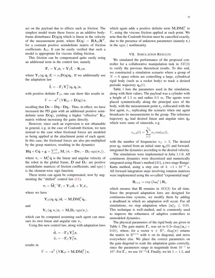
The physical parameters of the rigid body are given inTable I. The gain matrix Γo was set to 0.3∗ diag(|ao|+0.01), where, for a vector v ∈ Rn, diag(v) returnsthe matrix in Rn×n with v on its diagonal, and zeroseverywhere else. We place the correct parameters onthe gain diagonal to scale the adaptation gains correctly,since the parameters range in magnitude from 10−1 to104. For Γr, we use 10−3∗I. Finally, we let λ = 1.5, and

11

parameter value

m 1.89× 104 kg

Ixx 1.54× 104 kgm2

Iyy 1.54× 104 kgm2

Izz 2.37× 103 kgm2

rp [0, 0, 1.5] m

r1 [0, 0, 1.5] m

r2 [0, 0,−1.5] m

r3 [0.5, 0, 0] m

r4 [−0.5, 0, 0] m

r5 [0, 0.5, 0] m

r5 [0,−0.5, 0] m

TABLE I. Parameter Values for Simulation in SE(3)

KD = diag(KF ,KM ), where KF = 5× 104∗I, andKM = 5× 103∗I. The initial parameter estimates oi andri were drawn from zero-mean multivariate Gaussiandistributions with variances of Σo = I and Σr = 2I,respectively. Source code of the simulation is publiclyavailable at https://github.com/pculbertson/hamilton ac.

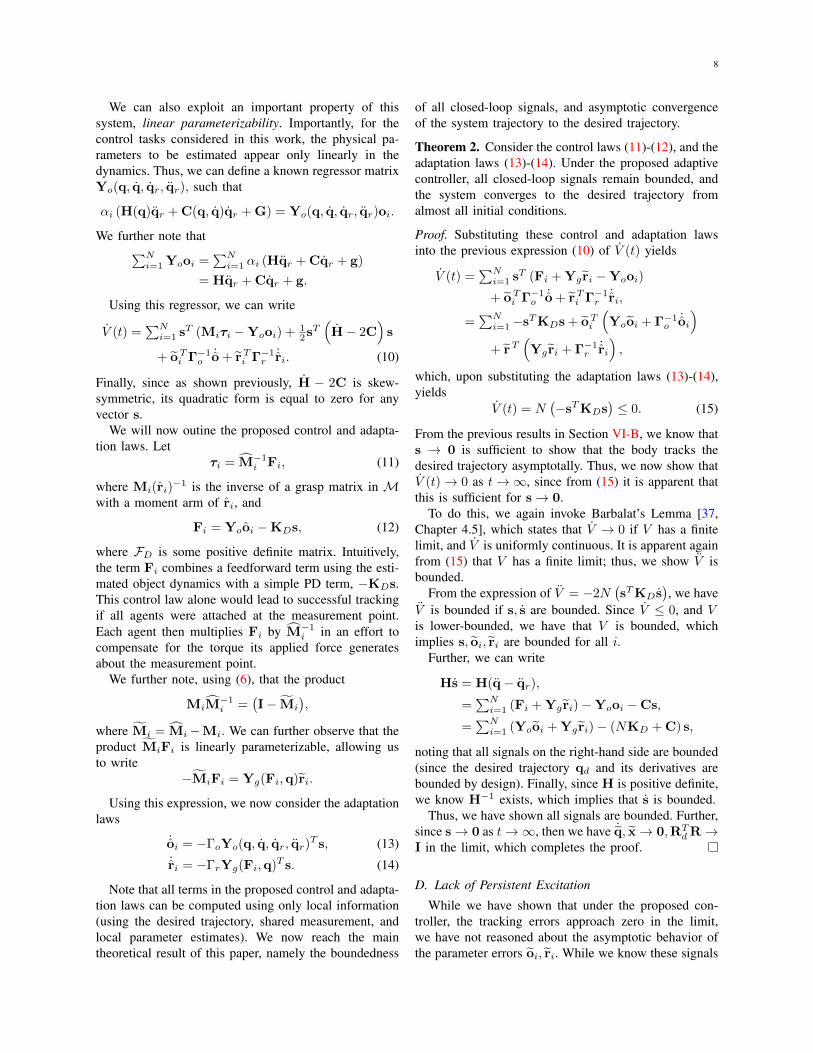
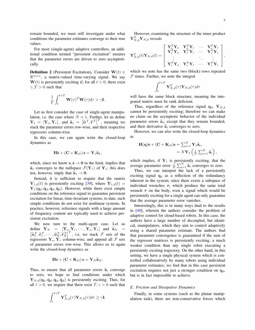
Figure 2 plots the error signals and Lyapunov functionvalue over the course of the simulation. We can see thatthe sliding variable is able to quickly reach the slidingsurface s = 0. Further, once on the sliding surface, wenotice the rotation error metric also converges to zero,implying R → Rd, as expected. We can further seethat the Lyapunov function V (t) is strictly decreasing(implying V (t) ≤ 0), and converges to a constant, non-zero value. This implies that the parameter errors oi, rido not converge to zero, which matches intuition due tothe lack of a persistently exciting signal, as shown inSection VI-D.

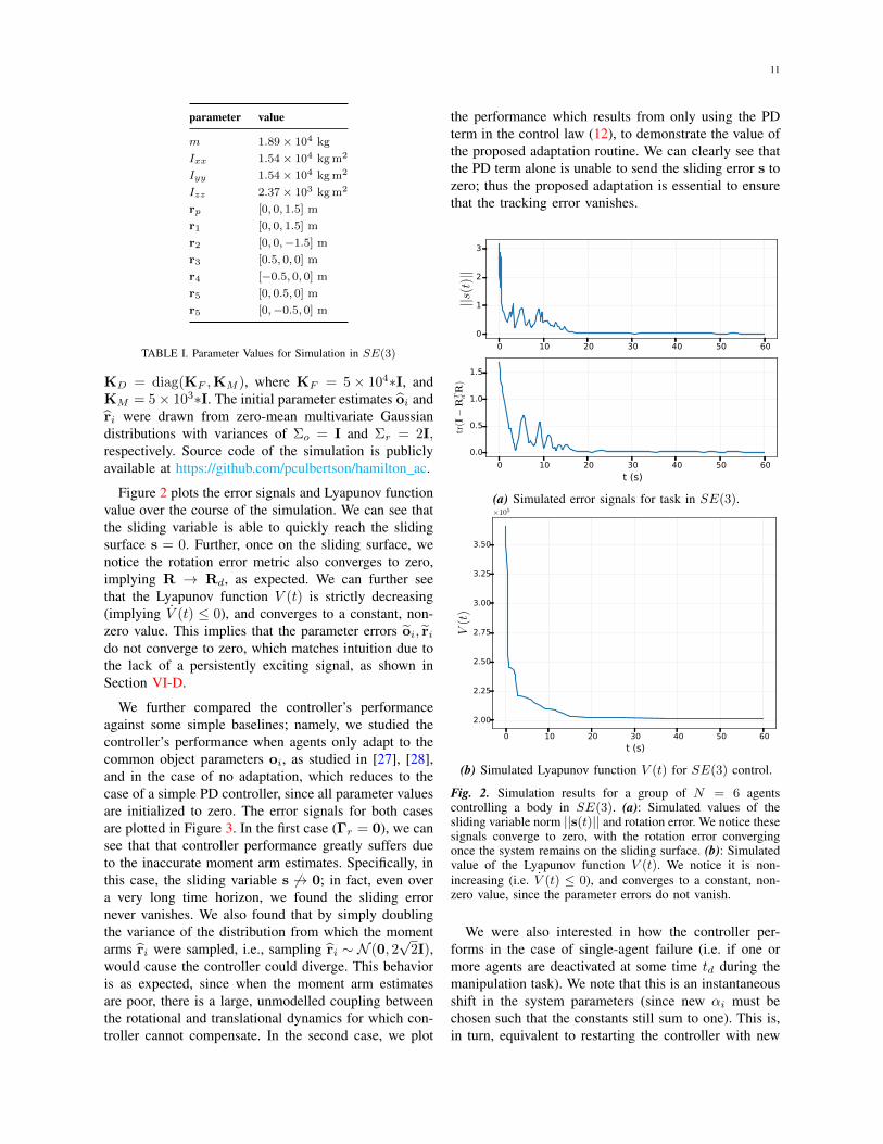
We further compared the controller’s performanceagainst some simple baselines; namely, we studied thecontroller’s performance when agents only adapt to thecommon object parameters oi, as studied in [27], [28],and in the case of no adaptation, which reduces to thecase of a simple PD controller, since all parameter valuesare initialized to zero. The error signals for both casesare plotted in Figure 3. In the first case (Γr = 0), we cansee that that controller performance greatly suffers dueto the inaccurate moment arm estimates. Specifically, inthis case, the sliding variable s 6→ 0; in fact, even overa very long time horizon, we found the sliding errornever vanishes. We also found that by simply doublingthe variance of the distribution from which the momentarms ri were sampled, i.e., sampling ri ∼ N (0, 2

√2I),

would cause the controller could diverge. This behavioris as expected, since when the moment arm estimatesare poor, there is a large, unmodelled coupling betweenthe rotational and translational dynamics for which con-troller cannot compensate. In the second case, we plot

the performance which results from only using the PDterm in the control law (12), to demonstrate the value ofthe proposed adaptation routine. We can clearly see thatthe PD term alone is unable to send the sliding error s tozero; thus the proposed adaptation is essential to ensurethat the tracking error vanishes.

0 10 20 30 40 50 600

1

2

3

||s(t

)||0 10 20 30 40 50 60

t (s)

0.0

0.5

1.0

1.5

tr(I−

RT dR

)

(a) Simulated error signals for task in SE(3).

0 10 20 30 40 50 60t (s)

2.00

2.25

2.50

2.75

3.00

3.25

3.50

V(t

)

×105

(b) Simulated Lyapunov function V (t) for SE(3) control.

Fig. 2. Simulation results for a group of N = 6 agentscontrolling a body in SE(3). (a): Simulated values of thesliding variable norm ||s(t)|| and rotation error. We notice thesesignals converge to zero, with the rotation error convergingonce the system remains on the sliding surface. (b): Simulatedvalue of the Lyapunov function V (t). We notice it is non-increasing (i.e. V (t) ≤ 0), and converges to a constant, non-zero value, since the parameter errors do not vanish.

We were also interested in how the controller per-forms in the case of single-agent failure (i.e. if one ormore agents are deactivated at some time td during themanipulation task). We note that this is an instantaneousshift in the system parameters (since new αi must bechosen such that the constants still sum to one). This is,in turn, equivalent to restarting the controller with new

12

0 10 20 30 40 50 60012345

||s(t

)||proposed

PD

mass only

0 10 20 30 40 50 60t (s)

0

1

2

tr(I−

RT dR

)

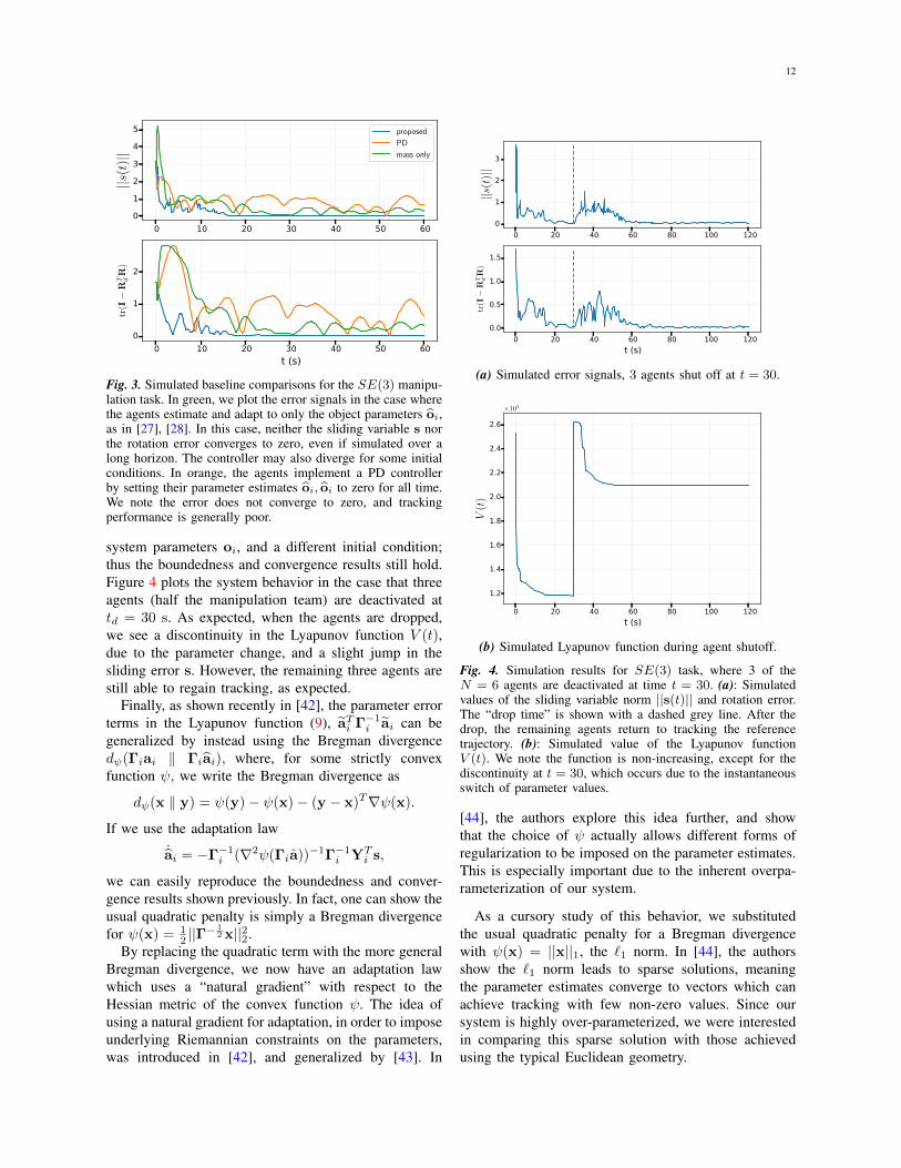
Fig. 3. Simulated baseline comparisons for the SE(3) manipu-lation task. In green, we plot the error signals in the case wherethe agents estimate and adapt to only the object parameters oi,as in [27], [28]. In this case, neither the sliding variable s northe rotation error converges to zero, even if simulated over along horizon. The controller may also diverge for some initialconditions. In orange, the agents implement a PD controllerby setting their parameter estimates oi, oi to zero for all time.We note the error does not converge to zero, and trackingperformance is generally poor.

system parameters oi, and a different initial condition;thus the boundedness and convergence results still hold.Figure 4 plots the system behavior in the case that threeagents (half the manipulation team) are deactivated attd = 30 s. As expected, when the agents are dropped,we see a discontinuity in the Lyapunov function V (t),due to the parameter change, and a slight jump in thesliding error s. However, the remaining three agents arestill able to regain tracking, as expected.

Finally, as shown recently in [42], the parameter errorterms in the Lyapunov function (9), aTi Γ−1i ai can begeneralized by instead using the Bregman divergencedψ(Γiai ‖ Γiai), where, for some strictly convexfunction ψ, we write the Bregman divergence as

dψ(x ‖ y) = ψ(y)− ψ(x)− (y − x)T∇ψ(x).

If we use the adaptation law˙ai = −Γ−1i (∇2ψ(Γia))−1Γ−1i YT

i s,

we can easily reproduce the boundedness and conver-gence results shown previously. In fact, one can show theusual quadratic penalty is simply a Bregman divergencefor ψ(x) = 1

2 ||Γ−12 x||22.

By replacing the quadratic term with the more generalBregman divergence, we now have an adaptation lawwhich uses a “natural gradient” with respect to theHessian metric of the convex function ψ. The idea ofusing a natural gradient for adaptation, in order to imposeunderlying Riemannian constraints on the parameters,was introduced in [42], and generalized by [43]. In

0 20 40 60 80 100 1200

1

2

3

||s(t

)||

0 20 40 60 80 100 120t (s)

0.0

0.5

1.0

1.5

tr(I−

RT dR

)

(a) Simulated error signals, 3 agents shut off at t = 30.

0 20 40 60 80 100 120t (s)

1.2

1.4

1.6

1.8

2.0

2.2

2.4

2.6

V(t

)

×105

(b) Simulated Lyapunov function during agent shutoff.

Fig. 4. Simulation results for SE(3) task, where 3 of theN = 6 agents are deactivated at time t = 30. (a): Simulatedvalues of the sliding variable norm ||s(t)|| and rotation error.The “drop time” is shown with a dashed grey line. After thedrop, the remaining agents return to tracking the referencetrajectory. (b): Simulated value of the Lyapunov functionV (t). We note the function is non-increasing, except for thediscontinuity at t = 30, which occurs due to the instantaneousswitch of parameter values.

[44], the authors explore this idea further, and showthat the choice of ψ actually allows different forms ofregularization to be imposed on the parameter estimates.This is especially important due to the inherent overpa-rameterization of our system.

As a cursory study of this behavior, we substitutedthe usual quadratic penalty for a Bregman divergencewith ψ(x) = ||x||1, the `1 norm. In [44], the authorsshow the `1 norm leads to sparse solutions, meaningthe parameter estimates converge to vectors which canachieve tracking with few non-zero values. Since oursystem is highly over-parameterized, we were interestedin comparing this sparse solution with those achievedusing the typical Euclidean geometry.

13

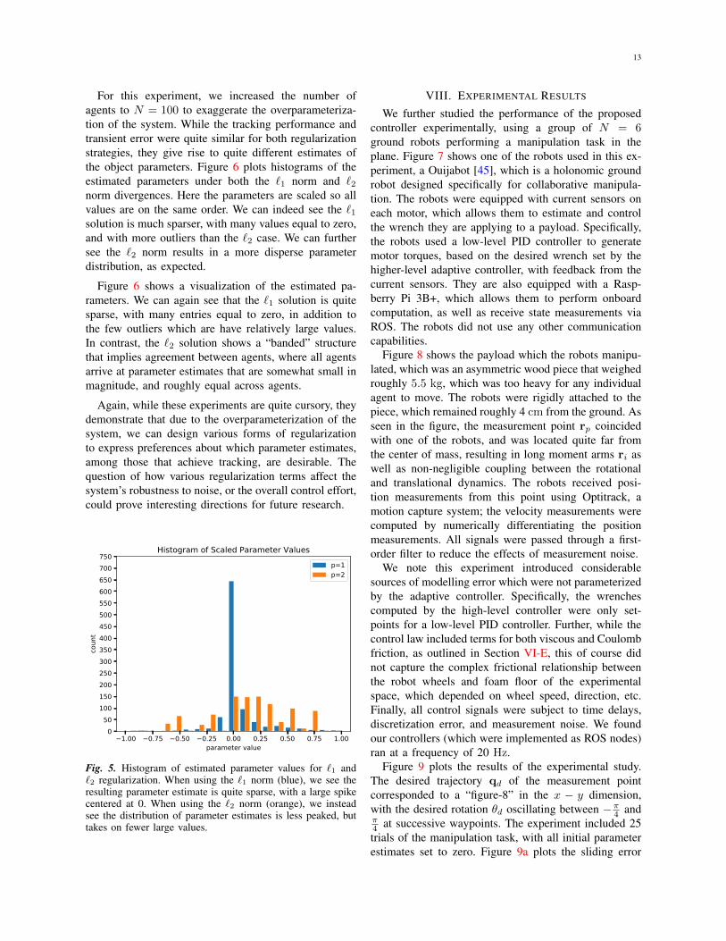
For this experiment, we increased the number ofagents to N = 100 to exaggerate the overparameteriza-tion of the system. While the tracking performance andtransient error were quite similar for both regularizationstrategies, they give rise to quite different estimates ofthe object parameters. Figure 6 plots histograms of theestimated parameters under both the `1 norm and `2norm divergences. Here the parameters are scaled so allvalues are on the same order. We can indeed see the `1solution is much sparser, with many values equal to zero,and with more outliers than the `2 case. We can furthersee the `2 norm results in a more disperse parameterdistribution, as expected.

Figure 6 shows a visualization of the estimated pa-rameters. We can again see that the `1 solution is quitesparse, with many entries equal to zero, in addition tothe few outliers which are have relatively large values.In contrast, the `2 solution shows a “banded” structurethat implies agreement between agents, where all agentsarrive at parameter estimates that are somewhat small inmagnitude, and roughly equal across agents.

Again, while these experiments are quite cursory, theydemonstrate that due to the overparameterization of thesystem, we can design various forms of regularizationto express preferences about which parameter estimates,among those that achieve tracking, are desirable. Thequestion of how various regularization terms affect thesystem’s robustness to noise, or the overall control effort,could prove interesting directions for future research.

1.00 0.75 0.50 0.25 0.00 0.25 0.50 0.75 1.00parameter value

050

100150200250300350400450500550600650700750

coun

t

Histogram of Scaled Parameter Valuesp=1p=2

Fig. 5. Histogram of estimated parameter values for `1 and`2 regularization. When using the `1 norm (blue), we see theresulting parameter estimate is quite sparse, with a large spikecentered at 0. When using the `2 norm (orange), we insteadsee the distribution of parameter estimates is less peaked, buttakes on fewer large values.

VIII. EXPERIMENTAL RESULTS

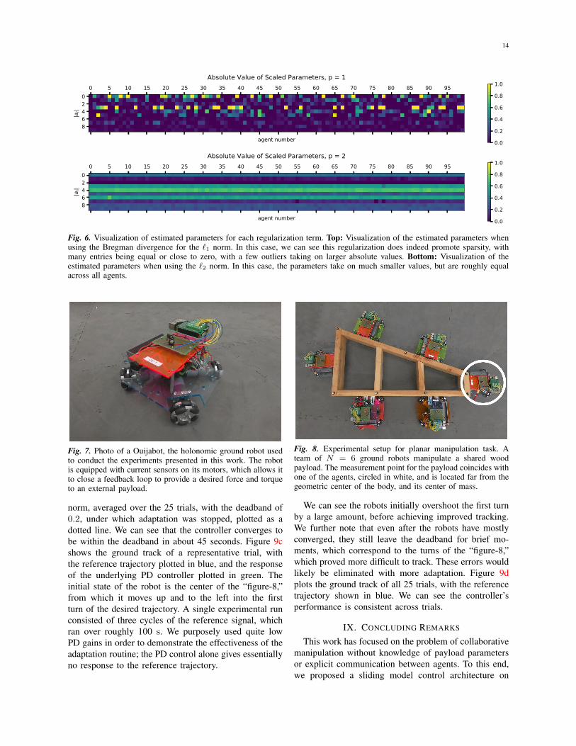
We further studied the performance of the proposedcontroller experimentally, using a group of N = 6ground robots performing a manipulation task in theplane. Figure 7 shows one of the robots used in this ex-periment, a Ouijabot [45], which is a holonomic groundrobot designed specifically for collaborative manipula-tion. The robots were equipped with current sensors oneach motor, which allows them to estimate and controlthe wrench they are applying to a payload. Specifically,the robots used a low-level PID controller to generatemotor torques, based on the desired wrench set by thehigher-level adaptive controller, with feedback from thecurrent sensors. They are also equipped with a Rasp-berry Pi 3B+, which allows them to perform onboardcomputation, as well as receive state measurements viaROS. The robots did not use any other communicationcapabilities.

Figure 8 shows the payload which the robots manipu-lated, which was an asymmetric wood piece that weighedroughly 5.5 kg, which was too heavy for any individualagent to move. The robots were rigidly attached to thepiece, which remained roughly 4 cm from the ground. Asseen in the figure, the measurement point rp coincidedwith one of the robots, and was located quite far fromthe center of mass, resulting in long moment arms ri aswell as non-negligible coupling between the rotationaland translational dynamics. The robots received posi-tion measurements from this point using Optitrack, amotion capture system; the velocity measurements werecomputed by numerically differentiating the positionmeasurements. All signals were passed through a first-order filter to reduce the effects of measurement noise.

We note this experiment introduced considerablesources of modelling error which were not parameterizedby the adaptive controller. Specifically, the wrenchescomputed by the high-level controller were only set-points for a low-level PID controller. Further, while thecontrol law included terms for both viscous and Coulombfriction, as outlined in Section VI-E, this of course didnot capture the complex frictional relationship betweenthe robot wheels and foam floor of the experimentalspace, which depended on wheel speed, direction, etc.Finally, all control signals were subject to time delays,discretization error, and measurement noise. We foundour controllers (which were implemented as ROS nodes)ran at a frequency of 20 Hz.

Figure 9 plots the results of the experimental study.The desired trajectory qd of the measurement pointcorresponded to a “figure-8” in the x − y dimension,with the desired rotation θd oscillating between −π4 andπ4 at successive waypoints. The experiment included 25trials of the manipulation task, with all initial parameterestimates set to zero. Figure 9a plots the sliding error

14

0 5 10 15 20 25 30 35 40 45 50 55 60 65 70 75 80 85 90 95

agent number

02468

|ai|

Absolute Value of Scaled Parameters, p = 1

0.0

0.2

0.4

0.6

0.8

1.0

0 5 10 15 20 25 30 35 40 45 50 55 60 65 70 75 80 85 90 95

agent number

02468

|ai|

Absolute Value of Scaled Parameters, p = 2

0.0

0.2

0.4

0.6

0.8

1.0

Fig. 6. Visualization of estimated parameters for each regularization term. Top: Visualization of the estimated parameters whenusing the Bregman divergence for the `1 norm. In this case, we can see this regularization does indeed promote sparsity, withmany entries being equal or close to zero, with a few outliers taking on larger absolute values. Bottom: Visualization of theestimated parameters when using the `2 norm. In this case, the parameters take on much smaller values, but are roughly equalacross all agents.

Fig. 7. Photo of a Ouijabot, the holonomic ground robot usedto conduct the experiments presented in this work. The robotis equipped with current sensors on its motors, which allows itto close a feedback loop to provide a desired force and torqueto an external payload.

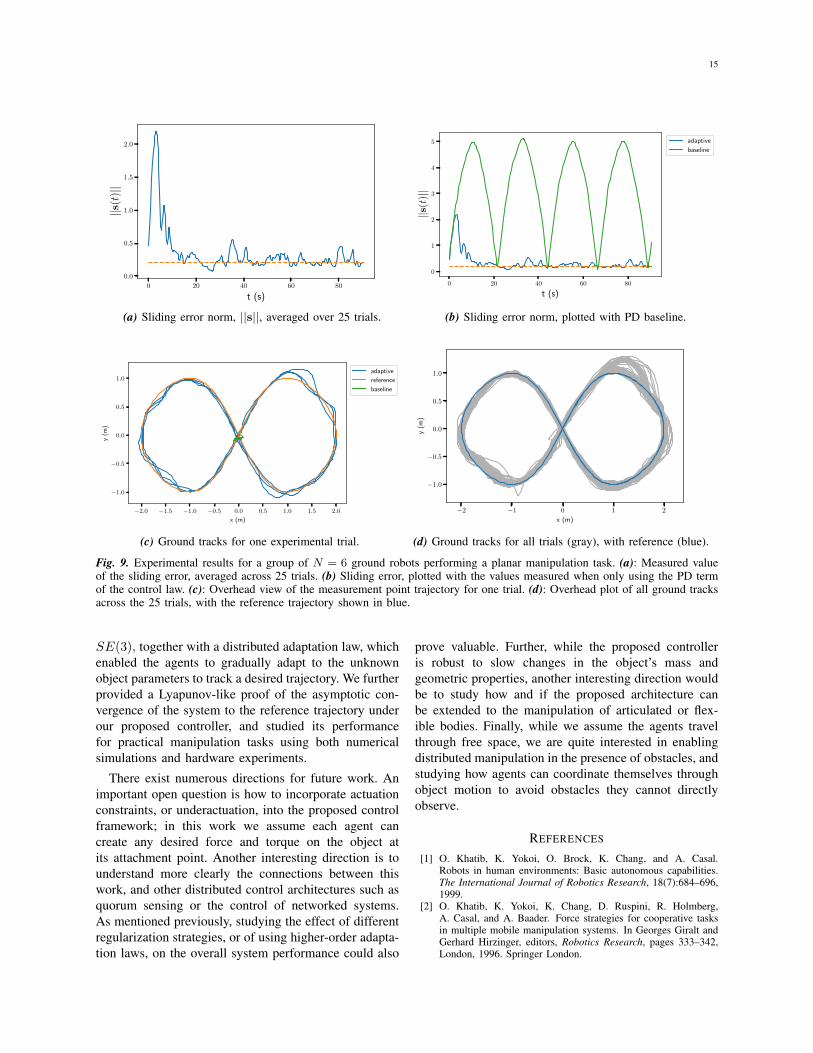
norm, averaged over the 25 trials, with the deadband of0.2, under which adaptation was stopped, plotted as adotted line. We can see that the controller converges tobe within the deadband in about 45 seconds. Figure 9cshows the ground track of a representative trial, withthe reference trajectory plotted in blue, and the responseof the underlying PD controller plotted in green. Theinitial state of the robot is the center of the “figure-8,”from which it moves up and to the left into the firstturn of the desired trajectory. A single experimental runconsisted of three cycles of the reference signal, whichran over roughly 100 s. We purposely used quite lowPD gains in order to demonstrate the effectiveness of theadaptation routine; the PD control alone gives essentiallyno response to the reference trajectory.

Fig. 8. Experimental setup for planar manipulation task. Ateam of N = 6 ground robots manipulate a shared woodpayload. The measurement point for the payload coincides withone of the agents, circled in white, and is located far from thegeometric center of the body, and its center of mass.

We can see the robots initially overshoot the first turnby a large amount, before achieving improved tracking.We further note that even after the robots have mostlyconverged, they still leave the deadband for brief mo-ments, which correspond to the turns of the “figure-8,”which proved more difficult to track. These errors wouldlikely be eliminated with more adaptation. Figure 9dplots the ground track of all 25 trials, with the referencetrajectory shown in blue. We can see the controller’sperformance is consistent across trials.

IX. CONCLUDING REMARKS

This work has focused on the problem of collaborativemanipulation without knowledge of payload parametersor explicit communication between agents. To this end,we proposed a sliding model control architecture on

15

0 20 40 60 80

t (s)

0.0

0.5

1.0

1.5

2.0

||s(t

)||

(a) Sliding error norm, ||s||, averaged over 25 trials.

0 20 40 60 80

t (s)

0

1

2

3

4

5

||s(t

)||

adaptive

baseline

(b) Sliding error norm, plotted with PD baseline.

−2.0 −1.5 −1.0 −0.5 0.0 0.5 1.0 1.5 2.0

x (m)

−1.0

−0.5

0.0

0.5

1.0

y(m

)

adaptive

reference

baseline

(c) Ground tracks for one experimental trial.

−2 −1 0 1 2

x (m)

−1.0

−0.5

0.0

0.5

1.0

y(m

)

(d) Ground tracks for all trials (gray), with reference (blue).

Fig. 9. Experimental results for a group of N = 6 ground robots performing a planar manipulation task. (a): Measured valueof the sliding error, averaged across 25 trials. (b) Sliding error, plotted with the values measured when only using the PD termof the control law. (c): Overhead view of the measurement point trajectory for one trial. (d): Overhead plot of all ground tracksacross the 25 trials, with the reference trajectory shown in blue.

SE(3), together with a distributed adaptation law, whichenabled the agents to gradually adapt to the unknownobject parameters to track a desired trajectory. We furtherprovided a Lyapunov-like proof of the asymptotic con-vergence of the system to the reference trajectory underour proposed controller, and studied its performancefor practical manipulation tasks using both numericalsimulations and hardware experiments.

There exist numerous directions for future work. Animportant open question is how to incorporate actuationconstraints, or underactuation, into the proposed controlframework; in this work we assume each agent cancreate any desired force and torque on the object atits attachment point. Another interesting direction is tounderstand more clearly the connections between thiswork, and other distributed control architectures such asquorum sensing or the control of networked systems.As mentioned previously, studying the effect of differentregularization strategies, or of using higher-order adapta-tion laws, on the overall system performance could also

prove valuable. Further, while the proposed controlleris robust to slow changes in the object’s mass andgeometric properties, another interesting direction wouldbe to study how and if the proposed architecture canbe extended to the manipulation of articulated or flex-ible bodies. Finally, while we assume the agents travelthrough free space, we are quite interested in enablingdistributed manipulation in the presence of obstacles, andstudying how agents can coordinate themselves throughobject motion to avoid obstacles they cannot directlyobserve.

REFERENCES

[1] O. Khatib, K. Yokoi, O. Brock, K. Chang, and A. Casal.Robots in human environments: Basic autonomous capabilities.The International Journal of Robotics Research, 18(7):684–696,1999.

[2] O. Khatib, K. Yokoi, K. Chang, D. Ruspini, R. Holmberg,A. Casal, and A. Baader. Force strategies for cooperative tasksin multiple mobile manipulation systems. In Georges Giralt andGerhard Hirzinger, editors, Robotics Research, pages 333–342,London, 1996. Springer London.

16

[3] O. Khatib, K. Yokoi, K. Chang, D. Ruspini, R. Holmberg, andA. Casal. Coordination and decentralized cooperation of multiplemobile manipulators. Journal of Robotic Systems, 13(11):755–764, November 1996.

[4] J. Fink, M. A. Hsieh, and V. Kumar. Multi-robot manipulationvia caging in environments with obstacles. In 2008 IEEEInternational Conference on Robotics and Automation, pages1471–1476, May 2008.

[5] D. Rus, B. Donald, and J. Jennings. Moving furniture with teamsof autonomous robots. In Proceedings 1995 IEEE/RSJ Inter-national Conference on Intelligent Robots and Systems. HumanRobot Interaction and Cooperative Robots. IEEE Comput. Soc.Press, 1995.

[6] C. Alford and S. Belyeu. Coordinated control of two robot arms.In Proceedings. 1984 IEEE International Conference on Roboticsand Automation, volume 1, pages 468–473, March 1984.

[7] Oussama Khatib. Object manipulation in a multi-effector robotsystem. In Proceedings of the 4th International Symposium onRobotics Research, pages 137–144, Cambridge, MA, USA, 1988.MIT Press.

[8] John T. Wen and Kenneth Kreutz-Delgado. Motion and forcecontrol of multiple robotic manipulators. Automatica, 28(4):729– 743, 1992.

[9] R. C. Bonitz and T. C. Hsia. Internal force-based impedancecontrol for cooperating manipulators. IEEE Transactions onRobotics and Automation, 12(1):78–89, Feb 1996.

[10] F. Caccavale, P. Chiacchio, A. Marino, and L. Villani. Six-dof impedance control of dual-arm cooperative manipulators.IEEE/ASME Transactions on Mechatronics, 13(5):576–586, Oct2008.

[11] S. Erhart, D. Sieber, and S. Hirche. An impedance-basedcontrol architecture for multi-robot cooperative dual-arm mobilemanipulation. In 2013 IEEE/RSJ International Conference onIntelligent Robots and Systems, pages 315–322, Nov 2013.

[12] S. Erhart and S. Hirche. Internal force analysis and load distribu-tion for cooperative multi-robot manipulation. IEEE Transactionson Robotics, 31(5):1238–1243, Oct 2015.

[13] Karl Bohringer, Russell Brown, Bruce Donald, Jim Jennings, andDaniela Rus. Distributed robotic manipulation: Experiments inminimalism. In Oussama Khatib and J. Kenneth Salisbury, edi-tors, Experimental Robotics IV, pages 11–25, Berlin, Heidelberg,1997. Springer Berlin Heidelberg.

[14] Peng Song and V. Kumar. A potential field based ap-proach to multi-robot manipulation. In Proceedings 2002 IEEEInternational Conference on Robotics and Automation (Cat.No.02CH37292), volume 2, pages 1217–1222 vol.2, May 2002.

[15] Siamak G. Faal, Shadi Tasdighi Kalat, and Cagdas D. Onal.Towards collective manipulation without inter-agent communi-cation. In Proceedings of the 31st Annual ACM Symposium onApplied Computing, SAC ’16, pages 275–280, New York, NY,USA, 2016. Association for Computing Machinery.

[16] Daniel Mellinger, Michael Shomin, Nathan Michael, and VijayKumar. Cooperative Grasping and Transport Using MultipleQuadrotors, pages 545–558. Springer Berlin Heidelberg, Berlin,Heidelberg, 2013.

[17] Koushil Sreenath and Vijay Kumar. Dynamics, control andplanning for cooperative manipulation of payloads suspendedby cables from multiple quadrotor robots. In Robotics: Scienceand Systems IX. Robotics: Science and Systems Foundation, June2013.

[18] Sarah Tang, Koushil Sreenath, and Vijay Kumar. Multi-robottrajectory generation for an aerial payload transport system. InNancy M. Amato, Greg Hager, Shawna Thomas, and MiguelTorres-Torriti, editors, Robotics Research, pages 1055–1071,Cham, 2020. Springer International Publishing.

[19] Nathan Michael, Jonathan Fink, and Vijay Kumar. Cooperativemanipulation and transportation with aerial robots. AutonomousRobots, 30(1):73–86, Jan 2011.

[20] B. E. Jackson, T. A. Howell, K. Shah, M. Schwager, andZ. Manchester. Scalable cooperative transport of cable-suspended

loads with uavs using distributed trajectory optimization. IEEERobotics and Automation Letters, 5(2):3368–3374, 2020.

[21] Zijian Wang and Mac Schwager. Force-amplifying n-robottransport system (force-ants) for cooperative planar manipulationwithout communication. The International Journal of RoboticsResearch, 35(13):1564–1586, 2016.

[22] Z. Wang, S. Singh, M. Pavone, and M. Schwager. Cooperativeobject transport in 3d with multiple quadrotors using no peercommunication. In 2018 IEEE International Conference onRobotics and Automation (ICRA), pages 1064–1071, May 2018.

[23] A. Franchi, A. Petitti, and A. Rizzo. Decentralized parameterestimation and observation for cooperative mobile manipulationof an unknown load using noisy measurements. In 2015 IEEEInternational Conference on Robotics and Automation (ICRA),pages 5517–5522, May 2015.

[24] A. Petitti, A. Franchi, D. Di Paola, and A. Rizzo. Decentralizedmotion control for cooperative manipulation with a team ofnetworked mobile manipulators. In 2016 IEEE InternationalConference on Robotics and Automation (ICRA), pages 441–446,May 2016.

[25] Yan-Ru Hu, Andrew A. Goldenberg, and Chin Zhou. Motionand force control of coordinated robots during constrained mo-tion tasks. The International Journal of Robotics Research,14(4):351–365, 1995.

[26] Z. Li, S. S. Ge, and Z. Wang. Robust adaptive control of coordi-nated multiple mobile manipulators. In 2007 IEEE InternationalConference on Control Applications, pages 71–76, Oct 2007.

[27] Yun-Hui Liu and Suguru Arimoto. Decentralized adaptive andnonadaptive position/force controllers for redundant manipulatorsin cooperations. The International Journal of Robotics Research,17(3):232–247, 1998.

[28] Christos K. Verginis, Matteo Mastellaro, and Dimos V. Di-marogonas. Robust quaternion-based cooperative manipulationwithout force/torque information**this work was supported bythe h2020 erc starting grand bu-cophsys, the swedish researchcouncil (vr), the knut och alice wallenberg foundation and theeuropean union’s horizon 2020 research and innovation pro-gramme under the grant agreement no. 644128 (aeroworks).IFAC-PapersOnLine, 50(1):1754 – 1759, 2017. 20th IFAC WorldCongress.

[29] Domenico Prattichizzo and Jeffrey C. Trinkle. Grasping, pages671–700. Springer Berlin Heidelberg, Berlin, Heidelberg, 2008.

[30] P. Culbertson and M. Schwager. Decentralized adaptive controlfor collaborative manipulation. In 2018 IEEE InternationalConference on Robotics and Automation (ICRA), pages 278–285,May 2018.

[31] Jean-Jacques E. Slotine and Weiping Li. On the adaptive controlof robot manipulators. The International Journal of RoboticsResearch, 6(3):49–59, 1987.

[32] Nicolas Tabareau, Jean-Jacques Slotine, and Quang-Cuong Pham.How synchronization protects from noise. PLoS ComputationalBiology, 6(1):e1000637, January 2010.

[33] Giovanni Russo and Jean Jacques E. Slotine. Global convergenceof quorum-sensing networks. Phys. Rev. E, 82:041919, Oct 2010.

[34] Christopher M. Waters and Bonnie L. Bassler. Quorum sens-ing: Cell-to-cell communication in bacteria. Annual Review ofCell and Developmental Biology, 21(1):319–346, 2005. PMID:16212498.

[35] S. P. Bhat and D. S. Bernstein. A topological obstruction to globalasymptotic stabilization of rotational motion and the unwindingphenomenon. In Proceedings of the 1998 American ControlConference. ACC (IEEE Cat. No.98CH36207), volume 5, pages2785–2789 vol.5, 1998.

[36] Richard M. Murray, Zexiang Li, and S. Shankar Sastry. AMathematical Introduction to Robotic Manipulation. CRC Press,December 2017.

[37] Jean-Jacques E. Slotine and Weiping Li. Applied NonlinearControl. Prentice-Hall, Inc., 1991.

[38] G. C. Gomez Cortes, F. Castanos, and J. Davila. Sliding motionson so(3), sliding subgroups. In 2019 IEEE 58th Conference onDecision and Control (CDC), pages 6953–6958, 2019.

17

[39] Jean-Jacques E. Slotine and Weiping Li. Theoretical issues inadaptive manipulator control. In Proceedings of the 5th YaleWorkshop on Applied Adaptive Systems Theory, 1987.

[40] P. M. Wensing and J. Slotine. Cooperative adaptive control forcloud-based robotics. In 2018 IEEE International Conference onRobotics and Automation (ICRA), pages 6401–6408, 2018.

[41] J. Stoer and R. Bulirsch. Introduction to Numerical Analysis.Springer New York, 1980.

[42] T. Lee, J. Kwon, and F. C. Park. A natural adaptive control law forrobot manipulators. In 2018 IEEE/RSJ International Conferenceon Intelligent Robots and Systems (IROS), pages 1–9, 2018.

[43] Patrick M. Wensing and Jean-Jacques E. Slotine. Beyond con-vexity – contraction and global convergence of gradient descent,2018.

[44] Nicholas M. Boffi and Jean-Jacques E. Slotine. Higher-orderalgorithms and implicit regularization for nonlinearly parameter-ized adaptive control, 2019.

[45] Zijian Wang, Guang Yang, Xuanshuo Su, and Mac Schwager.OuijaBots: Omnidirectional robots for cooperative object trans-port with rotation control using no communication. In DistributedAutonomous Robotic Systems, pages 117–131. Springer Interna-tional Publishing, 2018.

[46] Stephen Boyd and Lieven Vandenberghe. Convex Optimization.Cambridge University Press, 2004.

APPENDIX

A. Proofs of Matrix Properties

We can now discuss properties of H,C, and theirderivatives. We first show the positive definiteness of H.Physically, since the kinetic energy of the system can beexpressed as

K =1

2qTH(q)q,

we must have H(q) � 0, otherwise there exists q 6= 0with K = 0. For a block matrix of the form

M =

[A BBT C

],

using the properties of the Schur complement [46],we can say M � 0 if and only if A � 0 andC−BTA−1B � 0.

Thus, since mI � 0 by inspection, H � 0 if and onlyif S = RIpR

T +m(Rrp)×(Rrp)

× � 0.We further use the fact that

v×v× = vvT − (vTv)I,

to write

S = R(Icm ±m(rTp rp − rpr

Tp ))RT ,

= RIcmRT ,

and thus S � 0, since Icm � 0 for bodies of finite size.Thus, we conclude H � 0.

We can further show H − 2C is skew-symmetric,which can be understood as a matrix expression ofconservation of energy. Specifically, using the principleof conservation of energy, we can write

qT (τ − g) =1

2

d

dt

[qTH(q)q

].

Differentiating the right side yields

qT (τ − g) = qTHq + 12 qT Hq,

which, rearranging, results in

qT (H− 2C)q = 0,

which must hold true for all q. While the matrix C isnon-unique, there exist choices of C where H − 2Cis skew-symmetric, which is indeed the case for thissystem. Thus, we can view this matrix property as anexpression of conservation of energy. We now demon-strate this property for our choice of C.

H is given by

H =

[03 A−AT

AT −A ω×RIpRT −RIpRω

×

],

where A = mω×(Rrp)×, and using the fact R =

ω×R. Further,

H− 2C =

[03 −BB D

],

where B = BT = A + AT and D = −ω×RIpRT −

RIpRω× − m((Rrp)

×x)×. We can see H − 2C isskew-symmetric, since D is skew-symmetric, and theoff-diagonal blocks are symmetric and of opposite sign.