Embed Size (px)
Citation preview
Decentralization: A Cautionary Tale
Michael Kremer, Sylvie Moulin, Robert Namunyu
Poverty Action Lab Paper No. 10
April 2003
Decentralization: A Cautionary Tale
Work in Progress
Michael Kremer1, Sylvie Moulin, Robert Namunyu
April 15, 2003
Abstract
Kenya’s education system blends substantial centralization with elements of local control and school choice. This paper argues that the system creates incentives for local communities to build too many small schools; to spend too much on teachers relative to non-teacher inputs; and to set school fees that exceed those preferred by the median voter and prevent many children from attending school. Moreover, the system renders the incentive effects of school choice counterproductive by undermining the tendency for pupils to switch into the schools with the best headmasters. A randomized evaluation of a program operated by a non-profit organization suggests that budget-neutral reductions in the cost of attending school and increases in non-teacher inputs, financed by increases in class size, would greatly reduce dropout rates without reducing test scores. Moreover, evidence based on transfers into and out of program schools suggests that the population would prefer such a reallocation of expenditures.
1 Department of Economics, Harvard University, [email protected]. The authors thank Alicia Bannon, Elizabeth Beasley, Marcos de Carvalho Chamon, Alex Chan, Pascaline Dupas, Lynn Johnson, Ofer Malamud, and Courtney Umberger for excellent research assistance. We appreciate comments from Jens Ludwig and Jishnu Das. We are grateful for financial support from the World Bank. All errors are our own.
1
1. Introduction
Education and other social services are centralized in much of the developing
world. Many now advocate decentralization and community participation, and reforms
along these lines are increasingly being adopted.
This paper examines the experience of Kenya, which adopted elements of
decentralization and community participation in its educational system long before these
ideas became fashionable. Kenya’s system of financing local public goods, including
education, has great ideological importance in the country and is a key component of its
political economy. The word “harambee” is emblazoned on the national crest of Kenya
and on its currency. Literally translated as “let’s pull together,” harambee refers to the
system adopted under Kenya’s first president, in which local communities raise funds for
schools and other local public goods. Under the education system Kenya established
after independence, local harambee fundraisers typically cover initial capital costs for
new schools. School fees set by local school committees and collected by headmasters
cover most non-teacher recurrent costs, such as chalk, classroom maintenance, and
teachers’ textbooks. People who live within walking distance of more than one school –
a considerable portion of the population - are in practice free to choose which school
their children attend. Once local communities establish schools, the central government
assigns teachers to schools and pays their salaries. 2 It also sets the curriculum and
administers national tests at the end of primary and secondary school. Outside donors
supplement
2 Immediately after schools are established, parents may have to pay costs to cover teachers' salaries as well, but the central government takes this over quickly.
2
Kenyan finance, sometimes providing additional resources that are targeted to poor or
poorly performing schools.
The harambee system funds not only schools, but also other small-scale local
projects like local clinics, churches, and agricultural facilities. Barkan and Holmquist
(1986) report that 90% of residents are or have been involved in the harambee process.
Seventy-three percent of people participate in primary school projects and 63%
participate in secondary school projects (Barkan and Holmquist 1986). Wilson (1992)
finds that most projects are funded from catchment areas of less than 5 km radius.
Although the harambee system can be traced to pre-colonial era institutions, it
dovetails with much contemporary thinking about decentralization, community
participation, and school choice. The system utilizes local knowledge about which
projects are most needed and about each individual’s capacity to pay for these projects.
Relative to a system of centralized tax collection and expenditure determination, the
more decentralized harambee system gives local officials greater incentives to collect
funds from the population, and the local population more incentive to monitor the use of
these funds.
This paper first argues that interactions among the various elements of the school
finance system Kenya adopted at independence create perverse incentives. By financing
teachers at the central level but allowing local communities to start schools, the system
led to the construction of too many small schools; to excessive spending on teachers
relative to non-teacher inputs; and to the setting of school fees and other school
attendance requirements at a level that deters some from attending school and that
exceeds the level preferred by the median voter. Moreover, the school finance system
3
renders the incentives for headmasters created by competition under school choice
counterproductive and undermines tendencies for pupils to move to schools with the best
headmasters. We also argue that the decision to adopt the system set Kenya on a path that
led to growing fiscal costs and inefficiencies, the squeezing out of non-teacher
expenditures, and the eventual abandonment of the commitment to assign teachers to any
school created by a local community, freezing in place an inefficient and unequal
distribution of schools.
We then present evidence from a randomized evaluation of a program that paid
for textbooks, classroom construction, and the uniforms that parents in Kenyan schools
are required to purchase, which constitute the major cost to parents of sending their
children to school. The program led to a sharp reduction in dropout rates and a large
inflow of students from nearby schools into program schools, thus increasing the class
size in program schools by approximately 9 students. We find no significant effect of the
combination of higher pupil-teacher ratios and more non-teacher inputs on test scores.
Evidence from transfers suggests that overall, parents preferred the combination of lower
fees, more non-teacher inputs, and sharply higher pupil/teacher ratios associated with the
program. We then show that the Kenyan government could finance the textbooks,
classrooms, and reductions in cost of school to parents provided through the program
without external funds, by a much smaller increase in class size. Such a policy would
increase years of schooling by 17%.
The program also sheds light on the debate over user fees in education that is
active generally in development, but particularly active now in Kenya, given the new
government’s decision to abolish fees. While user fees have been widely advocated as a
4
way to relieve fiscal pressure on central governments and increase accountability of
schools to local communities, they have also been criticized for keeping children out of
school. The results in this paper suggest that reducing the cost of attending school can
greatly increase school participation.
This paper draws on the work of several authors who have previously examined
the harambee system. Wilson (1992) seeks to explain the puzzle of why people
voluntarily contribute to public goods through harambee, arguing that voluntary
provision can succeed in a repeated game in which participants know each other well and
contributions are publicized. In contrast, our analysis suggests that widespread
participation in the harambee system is due at least in part to massive subsidies from the
central government. Ngau (1987) documents and decries efforts by the central
government to control and regulate the harambee system, for example by imposing
construction standards and trying to shift the harambee movement from local to district-
wide or national projects. He sees this as disempowerment at the grassroots level. We
interpret increased central regulation as an effort to correct inherent distortions in the
Kenyan school finance system.
Our analysis is closest to those prepared not simply as academic pieces, but rather
as policy documents. Cohen and Hook (1986) discuss the recurrent cost implications of
the harambee system for the central government. We go beyond this to argue that the
system distorts the composition of educational expenditure and to document this
empirically. Deolalikar (1999) examines educational spending in Kenya as a whole,
rather than focusing on the harambee system. He shows that Kenya’s pupil-teacher ratios
are low for a country of its income level, that education budgets are concentrated on
5
teacher salaries, and that fewer children participate in school than would be expected
given Kenya’s relatively high public expenditure on education. We show that these all
can be seen as consequences of Kenya’s school finance system, and we present empirical
evidence that this pattern of expenditure is not only out of line with international norms,
but inefficient.
The remainder of the paper is organized as follows. Section 2 provides
background on the Kenyan political and educational system at independence and
discusses the adoption of the harambee system by Kenya’s first president, Jomo
Kenyatta. Section 3 models the distortions created by the Kenyan school finance system.
Section 4 describes the NGO program we analyze. Section 5 documents the program’s
effect on class size. Section 6 examines the effect of the program on enrollment, grade
completion, and school attendance. Section 7 examines the overall effect of the program
on test scores. Section 8 examines the transfers between schools that were induced by
the program and the evidence it provides for what the local population prefers. Section 9
argues that Kenya could finance the inputs provided by the program through much
smaller increases in class size than those associated with the program.
2. Jomo Kenyatta and the Adoption of the Harambee System
A number of reasons have been set forth for Kenyatta’s adoption of the harambee
system: the fiscal weakness of the state, a belief in decentralization and local control, and
historical traditions dating to the pre-colonial period (Ngau 1987) (Thomas 1987). In our
view a key factor lay in the political economy of Kenya at independence.
6
Prior to colonization, the region that became Kenya was inhabited by a variety of
different groups, some settled agriculturalists, others nomadic pastoralists, speaking
different languages, each with its own political system. Britain imposed a centralized
government on the country, allocated the most densely settled regions of the country to
the local indigenous groups, and took other more sparsely populated land, used by
pastoralists, for colonial settlement. Colonial settlers brought in farm laborers from other
regions of the country.
During the colonial period various Christian denominations competed to
proselytize, and these groups often established schools. Graduates could obtain jobs in
the lower ranks of the civil service. Schools were opened most rapidly in the agricultural
area around the capital the British established at Nairobi. However, by 1960 only 20% of
the adult population was literate (Deolalikar, 1999).
The British did not allow much local elected self-government in the colonial
period. Although they sometimes relied on local chiefs, these chiefs often had little
legitimacy. In many areas, there had not been any chiefs prior to the colonial period.
Hence at independence there were not strong independent elected institutions at the local
level that could serve as a counterweight to the national government.
One of the key issues at independence was whether to adopt a federal system,
with elected bodies at the provincial level, or a unitary centralized state. Two main
political parties formed on opposing sides of this issue: KANU, which had strong
constituencies among Kenya’s two largest, most highly educated, and most politically
mobilized ethnic groups, backed a unitary state. KANU’s main rival KADU, which had a
constituency among smaller, less politically influential groups, advocated a federal or
7
majimbo system. KANU won power and in 1964 KADU was merged into the ranks of
KANU. In 1966 Kenyatta appointed Daniel arap Moi, the former chairman of KADU, as
vice-president.
A reason some of the groups that supported KANU may have opposed federalism
was fear that it could lead to the emergence of local ethnic movements or parties that
might discriminate against members of other ethnic groups who had moved to these
regions to set up businesses, work for the government, or farm in areas where land was
not as scarce. During the colonial period some people had moved out of densely settled
Central province into areas used by nomadic groups where the British had set up colonial
farms. (In fact, in another more recent debate over federalism in Kenya, many opponents
saw majimbo or federalism as a code word for expulsion of certain groups from places
outside their home area.) It seems likely that if local elected bodies were established and
given authority to hire and fire teachers, some might discriminate against members of
ethnic groups from other regions of the country. At independence, the members of the
relatively educated groups which backed KANU were better off under a system in which
civil service positions were allocated according to educational qualifications than they
would have been if local elected bodies were in charge of hiring.
The adoption of a centralized system also increased the power of the national
leadership and reduced the chance that alternative leaders could develop a local power
base. To the extent that the allocation of funds was not totally rule based and that hiring
was not totally meritocratic, the system helped incumbent politicians in the national
government build patronage networks. Local candidates for parliament competed in large
part on the basis of their ability to organize and finance harambee projects and to obtain
8
support for them from the center. Well-connected local politicians could get the central
government to start assigning teachers to the school more rapidly.
At the same time, Kenya’s leaders believed in local input, and wanted community
participation. They chose a system that did not allow for elections at the provincial or
district levels or give power over teachers to local governments, but did allow for
community participation through school committees.
The government implicitly committed that if local communities raised funds, built
schools, and kept them functioning for a short period, the central government would
supply teachers. Teachers would be allocated so that there would be at least one teacher
for each grade; if there were more than a certain number of students in a grade (currently
55), then another teacher would be added. (In practice, there are sometimes long delays
before new teachers are assigned.) Initially, the central government also had programs to
provide some non-teacher inputs, such as textbooks, to schools. As discussed below,
these programs providing non-teacher inputs eroded over time due to the increasing
budget commitments for teachers implicit in the harambee system.
Relative to a system in which funds were allocated in proportion to population,
the system provided more school funding to the prosperous and politically well-
organized regions, which at the time of independence formed the heart of the KANU
coalition. The harambee system was formally equal, but since it allocated central funding
in proportion to the installed base of schools and in proportion to the funds that
communities raised locally to establish new schools, it automatically allocated education
expenditure to politically organized communities. Areas that were educationally more
advanced could continue to benefit from the system even after they had saturated their
9
communities with primary schools by conducting harambees to build secondary schools.
Ngau (1987) found that harambee contributions per capita varied widely by region. In
1979, contributions in Central Province were six times higher than in the impoverished
North Eastern Province, and three times higher than in Nyanza Province. Thomas (1987)
estimates that Central Province received 1/3 of the total national harambee contributions
(as of 1989 it accounted for 14% of Kenya’s population). Note also that the system is
more flexible than a system that simply distributes resources among ethnic groups
according to a fixed formula since it automatically adjusts to provide more resources to
communities that become more politically organized. This makes the system more able
to survive changes in underlying political power.
The system harnessed local energies and allowed groups that were willing to
partially finance new schools to obtain them, but because control over hiring, firing, and
assignment of teachers was done centrally on the basis of formal educational credentials
by the national Teachers’ Service Commission, there was little scope for local school
bodies to discriminate against teachers from other ethnic groups, which would have been
detrimental to the relatively well-educated groups that held disproportionate political
power at independence.
The system allowed the rapid expansion in education that Kenya certainly needed
at independence. At independence, Kenya had 6056 primary schools with a total
enrollment of 891,600 students. Fifteen years later, there were nearly 3 million students
in primary school. By 1990, there were 14,690 primary schools with an enrollment of
slightly over 5,000,000. In 1963 there were only 151 secondary schools, with a total
enrolment of 30,120 students. Fifteen years later there were 362,000 students in
10

secondary school. By 2001 there were nearly 3,000 secondary schools with a total
enrollment of 620,000 students. (www.kenyaweb.com/educ/primary.html and Killick
1981). In 1960, the adult literacy rate was 20%. By 1995, it had increased to 77%
(Deolalikar, 1999).
3. Incentive Effects of the Kenyan School Finance System
This section argues that the system of school finance Kenya adopted at
independence created incentives for construction of too many small schools, at least in
those communities that were able to solve collective action problems; for excessive
spending on teachers relative to non-teacher inputs; and for the setting of school fees and
other costs of attending school above the level that would be preferred by the median
voter. Moreover, the system distorted potentially useful incentives for teachers and
headmasters generated by school choice. We argue that the system adopted at
independence may not have been that distortionary initially, but it set Kenya on a path
that entailed ever higher per-pupil costs, the squeezing out of non-teacher expenditures,
and the eventual abandonment of the commitment to provide teachers to schools
established by communities, which froze in place an inequitable and inefficient
distribution of schools.
The model helps explain why people voluntarily contribute with such apparent
generosity to harambees, and why these harambees focus on construction, rather than
other inputs, such as textbooks. It can also help account for many of the responses of
people outside the local area to the system, including donations to harambees from
neighboring communities and the central government’s efforts to insist on construction
11
standards and to regulate harambees. Finally, it helps account for the differing positions
of the central government and local school committees on school fees.
3.1. Incentives for Excessive School Construction
We argue that this system created excessive incentives for local communities to
build schools, so that at least in areas where communities can solve collective action
problems, there will be too many small schools.
Consider a small community that does not have its own school, but that can send
its children to a nearby existing school. If the community builds its own school, their
children will walk shorter distances to school, and will likely enjoy smaller class sizes.
The new school will be under the control of the local clan/tribe and of the religious
denomination that establishes the school. People from the community who become
teachers will be able to obtain jobs near their homes, and prominent local citizens can
lead the school rather than simply playing a secondary role at another school. The local
community will bear only the construction costs of the new school, while the central
government will pay the (much greater) recurrent costs.
To more formally identify the conditions under which incentives to build new
schools will be too great, suppose there is an existing school in village 1 with school-age
population x1 and that the inhabitants of village 2 with school-age population x2 are
considering whether to build a school on their own. Denote the discounted value of
learning per pupil that takes place in a school with population x as L(x). The present
discounted cost of building and staffing a new school is S, but the inhabitants of village 2
bear only the cost µS. It is efficient to create a second school if
12
x1L(x1) + x2L(x2) – S > (x1 + x2)L(x1 + x2) - x2w, where w is the discounted per pupil
extra cost of walking to the existing school. The inhabitants of village 2 will be willing
to pay the cost of a harambee if x2L(x2) – µS > x2L(x1 + x2) – x2w. Local incentives to
build a school are therefore too great if (1 - µ)S > x1[L(x1) – L(x1+x2)]. The local
community has too much of an incentive to create a school to the extent that they pay
only part of the present discounted costs of operating the school, and too little incentive
to create a school to the extent that they ignore the positive externalities of reducing class
size in neighboring schools by drawing off pupils.
Building a school may create positive externalities for neighboring schools, but
neighboring communities may interact in a way that internalizes these externalities. For
example, a community may discriminate against outsiders (see Miguel [2000]), or it may
contribute to harambees held by neighboring communities that are seeking to build their
own facilities. The proportion of the present discounted cost of establishing a school
borne by the local community, µ, is likely less than 10% given that, as in most school
systems, teacher compensation accounts for the vast bulk of education expenses. In the
Kenyan case, teacher compensation accounts for more than 90% of expenses. Salaries
are typically high relative to per capita GDP in developing countries, as teachers are
highly educated relative to the rest of the population. Moreover, teachers in Kenya have
a strong union. Per capita GDP is about $340 dollars, while we estimate that teacher
compensation, including benefits, is approximately $2000 a year. The annualized cost of
building a high-quality classroom might be on the order of $130.3 The central
government therefore pays more than 90% of the cost of a new school.
3 Author’s calculations.
13
While the school finance system creates excessive incentives for local
communities to build schools, it does not necessarily create excessive incentives for
individuals to build schools, since the free-rider problem within the local community
must be set against the excessive incentives for school building at the community level.
In theory, these two forces might offset each other in a way that produces optimal
incentives for school building. In fact, it seems likely that some communities will be able
to make considerable progress in solving the collective action problem, while others will
not. Thus, for example, in Wilson’s model of harambee as a repeated game, there are
many Nash equilibria, and some communities may get in an equilibrium with excessive
investment, while others might be stuck with people contributing privately optimal
amounts in a single round game. Perhaps more important, some communities develop
political methods for resolving this problem, and others do not. For example, although
harambee is theoretically supposed to be voluntary, local government officials sometimes
use the power of the state to extract harambee contributions. A local politician who does
this successfully will raise the welfare of the area and may therefore be more likely to be
elected. Other politicians may enter an implicit deal with the electorate under which they
personally fund harambee projects and then repay themselves from rents they can extract
from their public position. However, at any given moment, some areas will be able to
organize around a political entrepreneur who can successfully undertake these activities,
and others will not. Thus, rather than immediately causing the construction of too many
schools all over Kenya, the system set in motion a process that led to the construction of
more and more schools over time, but still left significant areas where school
construction lagged behind.
14
Some prima facie evidence that the system led to the construction of too many
small schools with low pupil-teacher levels is provided by comparing Kenya to other
countries at its income level. In 1997, at the time the project took place, the average
pupil-teacher ratio in Kenyan primary schools was 29, while in secondary school it was
only 16 (Deolalikar, 1999).4 In contrast, the average primary pupil-teacher ratio in low-
income countries is 50 (World Development Indicators, 2001). A regression of primary
pupil-teacher ratio against real per capita GDP for selected African countries in 1995
shows that Kenya’s current pupil-teacher ratios would be expected in countries with 2-4
times more GDP per capita (Deolalikar, 1999).5 Of course, the existence of a gap
between pupil-teacher ratios in Kenya and other poor countries is consistent not only
with the possibility that Kenya’s pupil-teacher ratios are too low, but also with the
possibility that other poor countries’ ratios are too high or that all countries are choosing
optimally given their unique circumstances. The evidence from the evaluation below
provides evidence supporting the first possibility.
In the region of Kenya where our data come from, Busia and Teso districts, the
median distance from a school to the nearest neighboring school is 1.4 km. Busia and
Teso have enough schools that if the population were evenly spaced, the average walking
distance to a school would only be .88 km if schools were placed to minimize walking
4 As discussed below, the ratio increased after this point as the government imposed a hiring freeze. 5 Lakdawalla (2001) argues that when countries have a relatively low-skill workforce, teachers’ relative salaries will be high, because teaching requires people fairly high up the skill distribution, but that as the skill level in the population as a whole increases, teachers relative skill and relative wage falls. When most of the population is unskilled, and teacher salaries are relatively high, countries adopt high pupil-teacher ratios, but as relative teacher skill levels and salaries fall, societies substitute quantity for quality, and pupil-teacher ratios fall. Although Lakdawalla focuses on time-series comparisons within currently developed countries, a similar relationship holds in the cross-section comparing countries with different levels of education.
15
distance. To the extent the population is concentrated in particular areas and school
placement responds, average distance could be smaller.
In 1995, at the time the program we examine was launched, 34% of schools in the
sample area had an eighth grade enrollment of 15 or fewer, 11.46% of schools had
seventh grade enrollment of 15 students or less, and 26.43% of schools had seventh grade
enrollment of 20 students or fewer. More than 25% of sixth grades enrolled 21 students
or fewer. Classes in lower grades tend to be larger, and the youngest grades are
overcrowded. Figure 1 shows fthe location and eighth grade enrollment of all primary
schools in Busia and Teso. In some cases, two closely neighboring schools each have
very small enrollment in particular grades. For example, two schools with eighth grade
enrollments of five and nine students respectively were only 1.5 km away from each
other. If the two classes were merged, and the savings on teacher salaries were
distributed among those 14 students, each would receive $139, or 40% of Kenyan per
capita income. To put matters in perspective, the corresponding figure for the U.S.
would be $14,000. It seems unlikely that students are better off with the small class size
than they would be with the cash or increased expenditures on non-teacher inputs, such
as textbooks, given that expenditures on teachers are large relative to non-teacher
educational expenditures.
Note that while local school committees bear only a small fraction of the cost of
reducing class size by building additional schools and reducing the number of pupils per
teacher, they bear the full cost of non-teacher inputs, such as textbooks. Thus, it seems
likely that outcomes could be improved by shifting funding from teachers to
16
non-construction, non-teacher inputs.6 Teacher salaries account for 95-97% of Kenyan
public recurrent expenditures on primary education (Deolalikar 1999).7 A Ministry of
Education survey found a pupil-textbook ratio of 17 in primary schools in 1990.
According to the 1995 Primary School Census, on average 27% of the desks and 36% of
chairs required in primary schools were not available (Deolalikar, 1999).
3.2. Incentives for Excessive School Fees and Other Attendance Requirements
School fees are set by local school committees made up of the headmaster,
parents elected to represent families of children in each grade, local officials, and a
representative of the religious denomination that is sponsoring the school. In some
schools, the committee is inactive, and the headmaster has almost complete de facto
authority, while in other schools the school committee is active, independent, and
influential. In any case, headmasters have a great deal of discretion about how strictly to
collect school fees, and headmasters often wind up waiving most of the fees for
households that are unable or unwilling to pay it.
Once schools have been established, both headmasters and parent representatives
on school committees have incentives to set fees and other attendance requirements, such
as uniform requirements, at levels that deter the poorest households from participating in
school and that are greater than the median voter would prefer. Headmasters have little
6 Pritchett and Filmer (1999) note that OLS estimates in a variety of countries typically suggest that the marginal product per dollar of inputs like books is often 10 to 100 times higher than that of inputs like teacher salary. Of course these estimates may be subject to a variety of biases. 7 While teachers’ salaries are a large share of expenditures in most developing countries, they are particularly high in Kenya because not only are teacher salaries high, but pupil-teacher ratios are low due to the incentives to set up many schools.
17
incentive to set low school fees and attendance requirements, since this will attract more
students to a school, increasing the workload for the headmaster and teachers, but
typically will not attract additional resources to a school, given that, at least in the upper
grades, most schools are far from the 55 pupils required for another teacher to be
assigned. (This in turn is due to the high density of schools relative to population
induced by the excessive incentives for school construction discussed above.) Moreover,
even if enrollment in a grade exceeds 55 students, the central government may be
sluggish in assigning another teacher. (Evidence from the NGO project discussed below
suggests that increases in enrollment spur much less than proportional increases in the
number of teachers assigned to a school. The ratio of enrollment in program schools to
enrollment in comparison schools increased by 51%; the ratio of the number of classes
offered in program and comparison schools increased by 16%.)
Another reason headmasters may be reluctant to lower school fees and other
attendance requirements is that while there are generally few incentives for headmasters,
they are sometimes transferred to more or less desirable locations based on their school’s
performance, which is judged largely by the average score on the primary school leaving
exam (KCPE). Pupils at the margin of dropping out may perform worse than average on
exams. Also, larger class size may decrease test scores. Incentives for headmasters to
keep class size small are especially strong in the upper grades, since only students who
make it through grade 8 take the KCPE. Finally, setting high school fees and other
attendance requirements allows the school to provide more inputs, which may help it
raise test scores and improve learning, and in any case, help make the school a more
comfortable place to work, for example, by financing repair of leaky roofs.
18
Parents’ committees are also likely to be biased towards setting school fees and
other attendance requirements at levels above those that would be preferred by the
median voter in Kenya and may prevent some children from attending school. Since only
those parents who have children in school are represented on the school committee,
parents whose children do not attend school because they have been deterred by the fees
and other requirements, such as uniform purchase, do not have a say in setting fees.
Parents who care more than average about education are more likely to take the time to
participate in the school committee. Moreover, since the school committee has one
representative from the parents of students in each grade, and since upper grade classes
are typically much smaller than other classes, parents who have children in the upper
grades, who are more likely to come from relatively advantaged backgrounds, are over-
represented.
Some suggestive evidence that fees set by school committees are higher than
would be preferred by the typical household comes from the conflict between the central
government and schools over school fees. In 1974, the central government declared the
abolition of school fees. Fees then crept back in again through the back door as school
“activity” fees, “building” fees, “parent-teacher association” fees, etc. During the
presidential election campaign in 1997, the president announced that schools should not
charge fees and cancelled the practice exams that students take and with them the fee for
taking these exams. After the election, schools resumed charging fees. The government
19
again announced the abolition of fees during the 2002 election campaign. The timing of
these moves suggests that fees are greater than would be preferred by the median voter.8
Aside from school fees, uniforms are a key school attendance requirement. Pupils
in Kenyan schools are required to purchase uniforms, which cost about $6, a substantial
sum relative to per capita GDP, which is $340.
3.3. Distortions of Incentives Under School Choice
There is considerable school choice in the region we examine, with Miguel and
Gugerty [2002] reporting that one out of four families has a pupil in a school that is not
the closest to their house. School choice can potentially benefit students both by creating
incentives for headmasters and teachers to improve school performance and by creating
incentives for students to switch to schools with better headmasters and teachers.
Unfortunately, Kenya’s education finance system renders the incentives for headmasters
and teachers counterproductive. Moreover, one side effect of outside assistance is that it
can weaken incentives for pupils to move to schools with better headmasters.
Suppose that headmasters maximize some function of the total resources available
to the school, their effort, and the welfare of people in the area. As discussed above,
typical class size is usually low enough that the integer constraint on the number of
teachers is binding, and most schools will not be able to obtain more teachers by
attracting a few additional pupils, at least in the upper grades. Headmasters who exert
extra effort to raise the quality of their school will therefore simply attract more pupils
8 Note that while the model suggests that using funds from teachers to reduce school fees or fund non-teacher inputs would be useful, it is silent on the tradeoff between school fees and non-teacher inputs.
20
but will not obtain corresponding increases in resources to serve those pupils, because the
additional school fees paid by the students are very small compared with the funding
from the central government. School choice produces limited incentive for headmasters
unless money follows pupils.9 (With fewer schools, more schools would be close to the
margin of being able to hire additional teachers, and incentives would be stronger.) One
piece of prima facie evidence that headmasters and teachers face weak incentives lies in
their high absenteeism rates. Glewwe, Ilias, and Kremer (2002) find that teachers were
absent from school 20% of the time on surprise visits. Glewwe, Kremer, and Moulin
(2001) found that when surprise visits were made to 50 schools in Busia, teachers were
absent from the classroom 31-38% of the time.
Aside from any desirable incentive effects on headmasters, school choice can
create desirable incentives for selection of schools by students in the presence of
exogenous variation in headmaster quality. If headmaster quality varies among schools,
then it is likely to be efficient for the best headmaster to operate the largest school, and
school choice can lead to this. To see this, suppose that learning in school i is
where Y is total learning, Q is the quality of the headmaster, R is the
resources available in the school, and N is the number of pupils. Dividing by N gives
learning per pupil, which declines with class size, holding other inputs fixed. Q is defined
so that a headmaster of skill MQ can supervise a school with M times as many students
and resources with no diminution of per pupil learning. The assumption that resources
are complementary with headmaster quality seems reasonable since good headmasters
are likely to be able to supervise and motivate more teachers and bad headmasters are
βαβα −−= 1iiii NRQY
9 On the other hand, headmasters who exert effort and thereby increase the quality of their schools may be
21
more likely to misuse or even steal school funds.10 Under this complementarity
assumption, it is optimal to allocate resources and students in proportion to headmaster
quality. Under a school choice system (with no locational constraints), in which
resources are allocated in proportion to enrollment, optimizing households will choose
schools in proportion to headmaster quality. Thus under a system in which resources
follow students, school choice will lead to optimal allocation of both students and
resources. A planner who allocates resources, but not students, could mimic the optimal
allocation by allocating resources in proportion to headmaster quality, in which case
students will also sort themselves in proportion to headmaster quality. In the actual
Kenyan system, it is not clear whether the central government allocates resources in
proportion to headmaster quality, but better headmasters on average do get more
resources, because they are assigned to larger schools.
Unfortunately, one side effect of external assistance is that it may weaken the
tendencies for school choice to match more children and resources to strong headmasters.
Assistance from external donors is a much smaller portion of school finance than
government support or local finances, but it often focuses on particular schools. Even if
the schools were randomly chosen, the correlation between headmaster quality and
resources would be reduced by external assistance. In fact, external donors are
particularly likely to support poor or poorly performing schools, and often provide more
assistance per student in small schools, and this may create a negative correlation
between external assistance and headmaster quality. For example, the CSP program we
examine provided large amounts of resources to schools that were selected on the basis of
able to charge more to pupils.
22
having poor facilities initially. Similarly, the Jomo Kenyatta Foundation / World Bank
textbook program targeted poor schools. A U.K.-financed program provides teacher
training and financial support for anti-AIDS clubs in schools with low test scores in
neighboring Nyanza province. Poor schools are more likely to have bad headmasters,
because bad headmasters are generally less able to raise and manage money, and because
the government often promotes good headmasters to bigger, more developed schools and
assigns bad headmasters to poor schools as punishment.
Moreover, much of the externally financed support for schools is on a per-teacher
or per-school basis, and therefore provides more support per student to small schools.
For example, this is the case for training for headmasters under the PRISM program or
for teachers under the AIDS education program. However, since good headmasters
attract pupils, providing more assistance per pupil in small schools may cause more
students to switch into schools with bad headmasters.
Finally, external assistance to the weakest schools decreases the one significant
incentive for headmasters in the Kenyan school system. Headmasters have less reason to
fear transfer to poor schools if these schools are disproportionately likely to be assisted
by external donors, particularly because it may be easier for headmasters to capture part
of the funds raised by external donors than it is for them to capture locally raised funds.
External assistance is a small enough proportion of Kenyan school finance that it
is only a secondary determinant of incentives for school choice and teacher and
headmaster effort, and by focusing on areas like textbook provision, which are relatively
neglected it fills important gaps in the Kenyan school finance system, so it is almost
10 Note that if headmaster quality and resources were substitutes, then it would make sense to provide more
23
certainly beneficial overall. However, this analysis suggests that external assistance
should be targeted to poor areas, but not necessarily to the poor schools within those
areas, especially given the dense networks of schools in the area, the willingness of
families to send children to schools other than the closest school, and the fairly
homogenous poverty of rural Busia and Teso. Urban areas, in contrast, may be more
likely to have dramatic income variation within small geographic areas. If outside
organizations must target individual schools, they should explicitly consider the quality
of the school leadership, as well as the physical resources of the school.
3.4 The Transformation of the System
The system contained the seeds of its own destruction. While in the beginning the
system allowed many schools to be built at relatively low cost to the central government
and low cost in distortion of incentives, the recurrent cost implications for the central
government were unsustainable. The incentives for widespread school construction and
low pupil-teacher ratios led to very high spending on education. Recurrent Ministry of
Education expenditure as a percentage of net government recurrent expenditures, net of
interest payments, rose from 15% in the 1960s to 40% in 1997-98: Public spending on
education was 7.4% of GDP in the late 1990s, while health and agriculture spending
constituted only 1.5% of GDP. Indeed, Kenya spends a higher share of its GDP on
public education expenditures than any other low-income African country (Utz, 2002). A
comparison of public education expenditure and gross primary enrollment rates in
resources to weak headmasters.
24
African countries shows that Kenya has relatively low enrollment rates given the amount
of money it spends (Deolalikar 1999).
Several shocks exacerbated the imbalance between schools and pupils and the
financial burden on the state. First, Kenya’s economy has stagnated in recent decades,
reducing demand for education. The number of candidates taking the Kenya Certificate
of Primary Education exam, which comes at the end of primary school, declined from
298,280 in 1985 to 249,080 in 1996 (Deolalikar 1999). Second, in 1984, the government
increased the number of grades in primary school from 7 to 8. Since children drop out
between grades, grade eight classes are particularly small.
The move toward multi-party democracy in the 1980’s increased the bargaining
power of KNUT, the Kenya National Union of Teachers, which held a strike during the
election year of 1997, winning promised pay increases of 27% for the first year, with
smaller increases stipulated for the following years (Deolalikar, 1999). The government
later reneged on the out-year pay increases, and KNUT recently conducted another strike,
which led to an agreement to reinstate the pay increases.
Faced with rising teacher costs, the government discontinued programs to provide
schools with textbooks and other non-teacher inputs, raising costs for households. In spite
of high government expenditures on education, attending school therefore is a major
expense for households and, as argued below, this expense deters many from attending
school. Only 68.9% of children between the ages of 6 and 13 now attend school
(Deolalikar, 1999).
The rising inefficiencies and fiscal costs led the government to rein in the system.
This is our interpretation of the central government’s efforts, decried by Ngau (1987), to
25

change the focus of the harambee movement from local projects to district-wide projects,
such as district hospitals, and to insist on high construction standards for harambee
schools. Shifting the focus of the harambee movement to district-level projects reduces
tendencies toward excessive facility construction, since there can only be one district
hospital per district. Mandating higher quality construction than the local community
prefers may seem inefficient, given that local people may know more about the
appropriate way to build in their area, the availability of different construction materials,
and local weather conditions. However, imposing higher standards can mitigate the
tendencies for excessive school construction. Regulation proved inadequate, since it was
often left to local officials, who were happy to bring funding to their districts at the
expense of future national budgets.
Eventually the open-ended commitment to provide teachers to harambee schools
had to be abandoned. This was done in a way that froze in place an inefficient and
inequitable distribution of resources. It is difficult to affix a precise date to the erosion of
the system, but by the 1980s the government was no longer simply providing teachers to
all new harambee secondary schools. In 1998, as fiscal pressures became more severe
following the raise in teacher’s pay, the government simply instituted a hiring freeze,
rather than systematically close down classes that were below a particular size. This
locked in rents for current teachers, as well as the existing distribution of schools.
Presumably, there would have been strong political opposition to closing down small
schools and reallocating the teachers, both from communities that would lose their local
schools and from teachers who would lose their jobs or have to relocate. (It is not clear
why politicians seem much more willing to allocate new facilities based on political pork
26
barrel considerations than to shut down old facilities based on these considerations, but
this seems a general phenomenon worldwide.)
Because up to that point different regions had had varying success at solving the
free rider problem of soliciting harambee contributions, the resulting system
simultaneously contained areas where pupil-teacher ratios were high and areas where
they were low. While the national average pupil-teacher ratio was 29.1 in 1997, pupil-
teacher ratios across districts range from 14 to 45, with the 10th and 90th percentiles being
21 and 34. The variation in pupil-teacher ratios from one primary school to the next is
much larger, ranging from 10 to 60. As teachers retire and die in different proportions at
different schools, the hiring freeze has led to increasing misallocation of teachers across
schools over time. The AIDS epidemic has exacerbated the problem.
It is worth noting that the erosion of the system coincided not only with rising
costs, but also with the transfer of power from Kenyatta to Moi. To the extent that Moi
represented ethnic groups with less ability to conduct local fundraising on their own, his
constituency might have preferred central government direction of investment rather than
an open-ended commitment to match local fundraising.
4. Evidence from the Child Sponsorship Program
The analysis above suggests that, in areas where free rider problems can be
overcome, local communities will create too many small schools, rather than fewer,
larger schools, and that reallocating expenditures from teachers to non-teacher inputs and
reducing the cost of education could improve welfare.
27
Evidence on the tradeoff between pupil-teacher ratios, non-teacher inputs, and the
cost of attending school is provided by the Child Sponsorship Program (CSP), conducted
by International Christelijk Steunfonds (ICS), a Dutch non-governmental organization
working in Kenya. The program took place in Kenya’s Busia and Teso districts, a
densely settled agricultural region on the border of Uganda.11 In 1994, ICS selected
fourteen particularly poor schools as candidates for the CSP program based on
recommendations from the district education office, teachers and headmasters in the area,
and site visits by ICS staff. The average test score of the median school in the group of
fourteen candidate schools was around the 30th percentile in the district.12 While our
estimates should be internally valid for the type of schools we examine, in assessing
external validity, it is important to bear in mind that the schools are poorer and perform
worse on tests than the average school in the area.
The fourteen schools were then randomly divided into program and comparison
groups. Schools were matched into pairs, based on geographic division and on school
size within divisions. Within each pair of schools, school assignment to the treatment or
comparison group was decided by a coin toss. We have only limited data on the schools
from the period prior to the program, but program and comparison groups seem similar in
terms of their test scores and their socioeconomic status. Program students seem to score
slightly higher than comparison students on tests administered before the intervention,
but these estimates are not statistically significant. There was also no significant
11 The district of Busia was split into two districts, Busia and Teso, in late 1995. 12 This averages the median score in the primary school leaving exam from grade eight as well as the district-wide practice exam that was administered in grade six and in grade seven. According to Deolalikar (1999), Busia district ranked 16th out of 43 districts in terms of KCPE score in 1996.
28
difference in socioeconomic status, as estimated from a survey questioning students
about whether they have shoes, a watch, or a metal roof.
The program provided uniforms, textbooks, and classroom construction to the
seven treatment schools beginning in 1995. All children in treatment schools were
provided with uniforms in the first three years of the program. In the fourth and fifth
years, half of the grades were provided uniforms in each year (students that received
uniforms in Year 4 did not receive uniforms in Year 5.) Ordinarily, Kenyan parents are
required to purchase uniforms for their children; these cost approximately $6, and might
be used for two years, so the program substantially reduced the cost of attending school.13
ICS gave program schools an extra $3.44 worth of textbooks per student in an
average year. ICS built ten classrooms in each program school over the course of five
years, with two classrooms being built every year after the first year. None of the
classrooms built were ready to use until Year 2. In some years, the community provided
some contribution, such as paying for the painting. Finally, beginning in Year 3, ICS
started providing a Christmas party to treatment schools.
Medical treatment and training was provided for both treatment and comparison
schools. These included monthly visits from a nurse and basic medical supplies such as
aspirin, bandages, and malaria medicine.14 Since these benefits accrued to both
treatment and comparison schools, we are not evaluating their impact, but instead, are
evaluating the effect of the other inputs, conditional on these.
As discussed in more detail below, we find that students in treatment schools had
13 The uniforms ICS provided were of higher quality than normal uniforms and cost somewhat more. 14 Also, teachers in both treatment and comparison schools received gifts such as soap or blankets as tokens of appreciation for their cooperation.
29
remained enrolled an average of 0.5 years longer after five years and advanced an
average of 0.3 grades further than their counterparts in comparison schools. Moreover,
school participation was higher in treatment schools than in comparison schools,
suggesting that parents were not merely enrolling their children in school to receive free
uniforms, but actually sending them to school.
The program not only led to greater retention of existing students, but it also
attracted many students from neighboring schools. We estimate that the average
treatment class had 8.9 more students than it would have had in the absence of the
intervention. ICS sought to restrict these inflows, in part to control disruption and
crowding. Our sample size is too small and there is too much selective attrition in the
sample to accurately estimate the program’s effect on test scores, but it seems likely that
any effect was modest. An estimate that tries to correct for selective attrition suggests the
overall effect on learning was small and positive.
A simple model in which new pupils transfer into treatment schools until the
benefits of the textbooks and reduced school fees offset the cost of overcrowding and the
costs of transferring to schools suggests that the benefits of the inputs provided by the
CSP program are more than sufficient to offset an increase in class size by 8.9 pupils.
The CSP program thus provides an opportunity to examine the effect of simultaneously
increasing class size, providing textbooks, and reducing the cost of school. The joint
impact of the changes made under the CSP program was to significantly improve
enrollment and grade advancement. The school choices of households in the area
indicate households were willing to accept an increase in class size of at least 8.9
students in exchange for the extra non-teacher inputs and lower costs under the program.
30
In section 8, we show that the Kenyan government could have financed the textbooks,
classroom construction, and uniforms provided by the CSP program without external
funds, using the savings that would be generated from an increase in class size much
smaller than that associated with the CSP program.15 This is consistent with a model in
which the trade-offs among class size, non-teacher inputs, and cost of attending school
are distorted, as argued in section 1.
Although the model suggests that both transferring resources from teachers to
non-teacher inputs and transferring resources from teachers to lowering the cost of school
would improve welfare, we only have one experiment, and therefore we cannot
separately determine the effect of each change. However, we can evaluate the combined
expenditure reallocation created by the CSP program.
5. Program Effect on Class Size
The program increased class size both because students in program schools
remained enrolled longer and because many students transferred in from neighboring
schools. The number of classes being offered at program schools increased only
modestly, and hence the program led to substantial increases in class size in the treatment
schools.16 Our enrollment data from Years 0-3 comes from the school register records
which schools themselves maintain. For Years 4 and 5, ICS conducted unannounced
15 In the CSP program, ICS paid for the assistance but did not realize the savings that accrued from the increased class size. Instead, savings in the per-pupil teachings costs for program schools were effectively captured by neighboring schools that which experienced a reduction in the pupil-teacher ratio. 16 Class size is not the same as the ratio of pupils to teachers in the school, because often the number of teachers assigned to a school is greater than the number of classes. For example, a school offering one class each in grades 1 through 8 would typically be assigned nine teachers.
31
school visits in order to see who was actually present in school on a given day, for the
purposes of keeping the list of enrolled students updated and measuring attendance. This
data is probably more accurate, since schools receiving lots of transfer students may have
delayed listing them on the register, either because of procedural delays or because ICS
was pressuring them not to accept too many transfer students. Before the intervention,
program schools had 9% more students than comparison schools, but by Year 2, they had
almost 69% more students (Table 1).17 Most of that increase was due to a substantial
inflow of students from neighboring schools.
Class size in grades 1-7 increased by 8.9 students despite an average increase of
.27 classes offered per grade in each school. Table 2 shows the average class size for the
program and comparison schools before and after the intervention. School register data
for Years 1-3 suggest an increase in class size of 4.1 students. Years 4 and 5 show an
increase in class size of 8.9 students on a base of around 29 students. Since class size
results from both student enrollment and teacher postings, it can fluctuate from one year
to the next as each group responds to the trend of the other. In grades 3 to 8, the ones for
which we have data on test scores, the program increased class size by 11.2 pupils. Few
students transferred between the program and comparison schools. Only 14 students who
were enrolled in program schools in 1994 ever enrolled in a comparison school.
Similarly, only 7 students ever transferred from comparison to program schools. The
downward trend in class size for the comparison schools cannot be attributed to such
transfers.
17 Enrollment data up to Year 3 is based on registers used to determine the initial list of students in our sample. Data from Year 4 on is based on visits in which the names of all children in school were recorded. Since the ratio of the enrollment in treatment and comparison schools seems comparable between Years 2 –
32
6. Program Impact on Years of Schooling and Grade Attainment
This section documents that students in treated schools remained enrolled for
longer and advanced more grades than students in comparison schools.
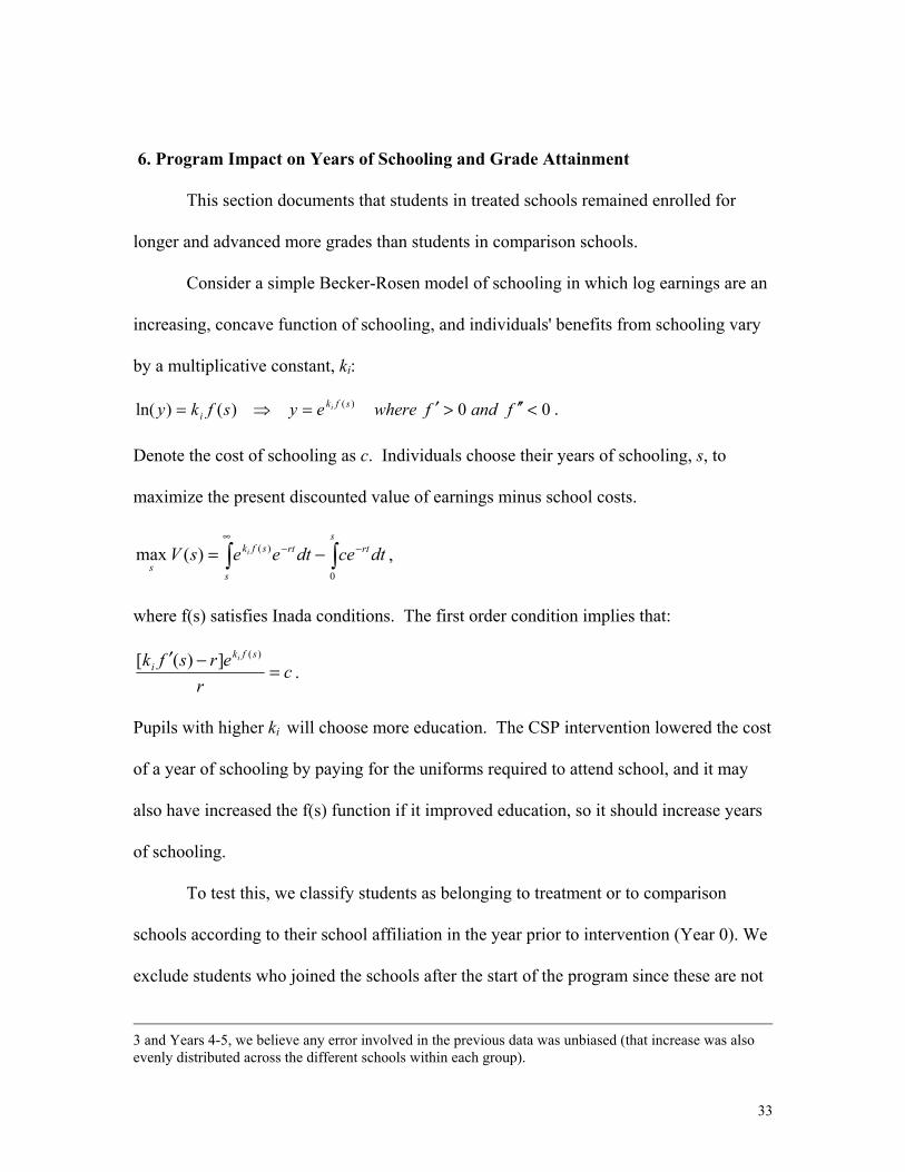
Consider a simple Becker-Rosen model of schooling in which log earnings are an
increasing, concave function of schooling, and individuals' benefits from schooling vary
by a multiplicative constant, ki:
00)()ln( )( <′′>′=⇒= fandfwhereeysfky sfki
i .
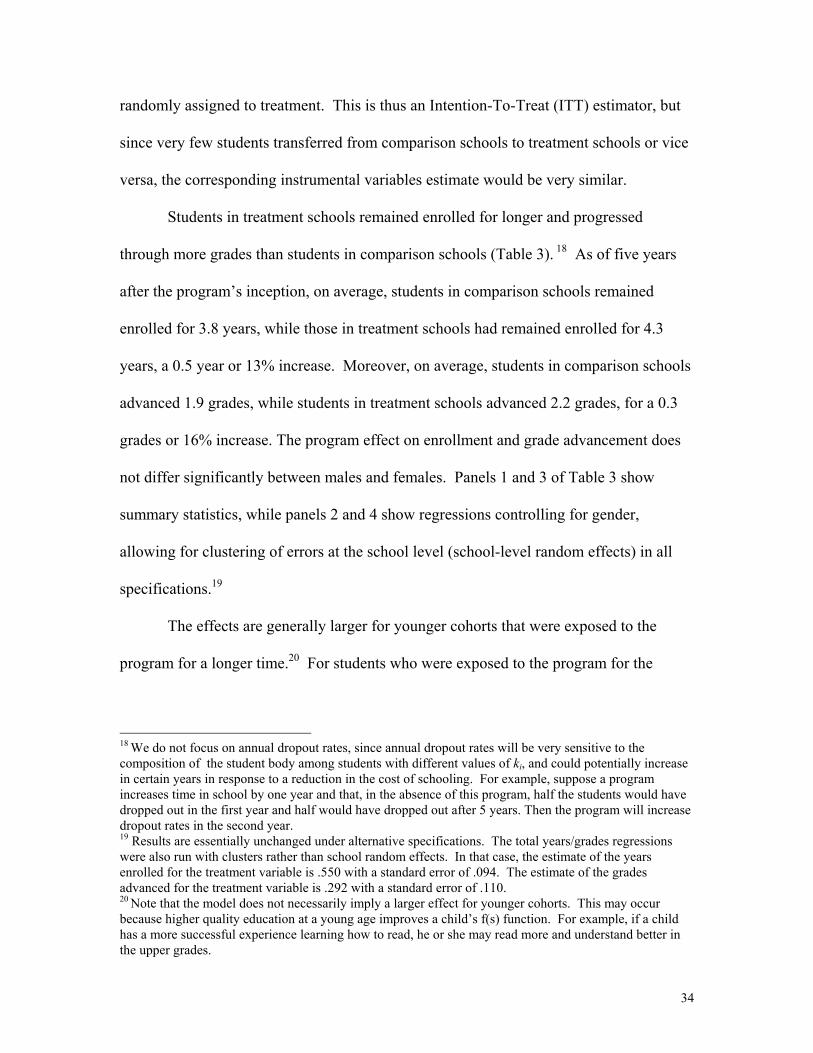
Denote the cost of schooling as c. Individuals choose their years of schooling, s, to
maximize the present discounted value of earnings minus school costs.
∫∫ −∞
− −=s
rt
s
rtsfk
sdtcedteesV i
0
)()(max ,
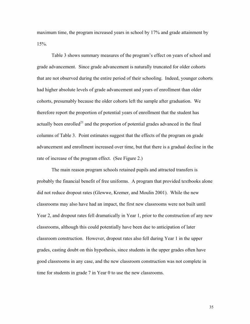
where f(s) satisfies Inada conditions. The first order condition implies that:
cr
ersfk sfki
i
=−′ )(])([
.
Pupils with higher ki will choose more education. The CSP intervention lowered the cost
of a year of schooling by paying for the uniforms required to attend school, and it may
also have increased the f(s) function if it improved education, so it should increase years
of schooling.
To test this, we classify students as belonging to treatment or to comparison
schools according to their school affiliation in the year prior to intervention (Year 0). We
exclude students who joined the schools after the start of the program since these are not
3 and Years 4-5, we believe any error involved in the previous data was unbiased (that increase was also evenly distributed across the different schools within each group).
33
randomly assigned to treatment. This is thus an Intention-To-Treat (ITT) estimator, but
since very few students transferred from comparison schools to treatment schools or vice
versa, the corresponding instrumental variables estimate would be very similar.
Students in treatment schools remained enrolled for longer and progressed
through more grades than students in comparison schools (Table 3). 18 As of five years
after the program’s inception, on average, students in comparison schools remained
enrolled for 3.8 years, while those in treatment schools had remained enrolled for 4.3
years, a 0.5 year or 13% increase. Moreover, on average, students in comparison schools
advanced 1.9 grades, while students in treatment schools advanced 2.2 grades, for a 0.3
grades or 16% increase. The program effect on enrollment and grade advancement does
not differ significantly between males and females. Panels 1 and 3 of Table 3 show
summary statistics, while panels 2 and 4 show regressions controlling for gender,
allowing for clustering of errors at the school level (school-level random effects) in all
specifications.19
The effects are generally larger for younger cohorts that were exposed to the
program for a longer time.20 For students who were exposed to the program for the
18 We do not focus on annual dropout rates, since annual dropout rates will be very sensitive to the composition of the student body among students with different values of ki, and could potentially increase in certain years in response to a reduction in the cost of schooling. For example, suppose a program increases time in school by one year and that, in the absence of this program, half the students would have dropped out in the first year and half would have dropped out after 5 years. Then the program will increase dropout rates in the second year. 19 Results are essentially unchanged under alternative specifications. The total years/grades regressions were also run with clusters rather than school random effects. In that case, the estimate of the years enrolled for the treatment variable is .550 with a standard error of .094. The estimate of the grades advanced for the treatment variable is .292 with a standard error of .110. 20 Note that the model does not necessarily imply a larger effect for younger cohorts. This may occur because higher quality education at a young age improves a child’s f(s) function. For example, if a child has a more successful experience learning how to read, he or she may read more and understand better in the upper grades.
34
maximum time, the program increased years in school by 17% and grade attainment by
15%.
Table 3 shows summary measures of the program’s effect on years of school and
grade advancement. Since grade advancement is naturally truncated for older cohorts
that are not observed during the entire period of their schooling. Indeed, younger cohorts
had higher absolute levels of grade advancement and years of enrollment than older
cohorts, presumably because the older cohorts left the sample after graduation. We
therefore report the proportion of potential years of enrollment that the student has
actually been enrolled21 and the proportion of potential grades advanced in the final
columns of Table 3. Point estimates suggest that the effects of the program on grade
advancement and enrollment increased over time, but that there is a gradual decline in the
rate of increase of the program effect. (See Figure 2.)
The main reason program schools retained pupils and attracted transfers is
probably the financial benefit of free uniforms. A program that provided textbooks alone
did not reduce dropout rates (Glewwe, Kremer, and Moulin 2001). While the new
classrooms may also have had an impact, the first new classrooms were not built until
Year 2, and dropout rates fell dramatically in Year 1, prior to the construction of any new
classrooms, although this could potentially have been due to anticipation of later
classroom construction. However, dropout rates also fell during Year 1 in the upper
grades, casting doubt on this hypothesis, since students in the upper grades often have
good classrooms in any case, and the new classroom construction was not complete in
time for students in grade 7 in Year 0 to use the new classrooms.
35
We also tried to track a few non-educational, long-term outcomes. Together with
Christel Vermeersch, we conducted a follow-up survey in August of 2001 on the cohort
of pupils who were in grade 4 in 1994. We found information on 474 of the original 574
students. At that point, 42% of girls from comparison schools were married, while only
30% of girls from program schools were married. This effect was not statistically
significant, given our sample size (t-value of –1.49). There was no significant effect on
the likelihood boys were married or on the number of children the former students have.
We are currently following up additional cohorts.
7. Effect on Test Scores It is difficult to make strong statements regarding the effect of the program on
learning, both because the sample of schools is small, giving large standard errors, and
because the composition of the sample changed radically. As discussed in the previous
section, many more students dropped out of comparison schools than treatment schools,
and hence we have many more test scores for treatment pupils. Estimates that do not
correct for this differential attrition yield an insignificant negative effect of the program
on test scores, while attempts to correct for this yield an insignificant positive estimate.
Beginning in Year 1, yearly exams were administered to students enrolled in grades 3
through 8 at the end of each school year. The test scores were normalized by subtracting
the mean score in comparison schools and dividing by the standard deviation of the
scores in the comparison schools, so that the comparison schools have a mean score of 0
and a standard deviation of 1.
21 Students enrolled for longer than the potential number of years required for continuous advancement (because they were retained) are counted as staying in school the maximum possible number of years.
36
Test score regressions include dummy variables for each subject, grade and year
interaction as well as for the pupil’s sex. As in previous sections, we use an intention to
treat analysis in which pupils who are in the comparison group schools in Year 0 are
classified as comparison pupils, and pupils in treatment schools in Year 0 are classified
as treatment pupils.
Table 4 presents estimates of the program’s effect on test scores. Regressions
allow for correlated error terms at the level of the school, interaction of school and
standard, interaction of school, standard and year, interaction of school, standard and
subject, and student. Dummies for the interactions of year, subject, and standard were
also included. Specification (i) of Table 4 presents an estimate of the program’s effect on
test scores, using all available test observations. This specification does not correct for
attrition bias, and hence is likely downward biased. The pool of students in program
schools likely deteriorated since students that would have otherwise dropped out
remained in school. If weaker students are more likely to drop out, then some of the
weak students who would have dropped out in the absence of the program will end up
staying in school. As time progresses, the proportion of test scores available for students
in the comparison schools relative to those in the treatment schools steadily declines. For
example, while in Year 1 the treatment group accounted for 57% of the 6208 test score
observations, by Year 4 it accounted for 62% of the 3979 observations. Thus, there is a
substantial decline in the number of observations over the years, which falls
disproportionately in the comparison group. The estimated program effect is negative but
insignificant. Specification (ii) uses a sample that includes only the test scores for
students who had progressed to that exam without being retained since the beginning of
37
the program and thus took the same test as other students initially enrolled in their grade
prior to the program that have also not been retained. Because students frequently repeat
grades in rural Kenya, this requirement excludes a large proportion of students, especially
those whose academic performance is not very strong. Since the students in this sample
are on average stronger than in the sample from specification (i), they are less likely to be
among the marginal cases whose drop out decision is influenced by the program. Thus,
this specification is less downward biased than (i). In fact, the share of test score
observations from the treatment group actually declines from 58% in Year 1 to 53% in
Year 4. But this specification leads to a very large loss in the number of observations. For
example, there were only 639 test score observations in Year 4. The estimated program
effect is negative but not significant, and higher than that of specification (i).
ICS administered its own test in Year 6 which was the same for all grades in order
to correct for the problem of grade repetition. The sample has 1230 subject test scores in
English and Math from 623 students who were mainly in grades 2 and 3 in 1994 and
were successfully tracked down in 2000. Specification (iii) shows the results of this test,
that also yields a negative but insignificant program effect.
Specification (iv) attempts to correct for attrition by imputing test scores for
repeaters and missing students. Repeaters took the exam for the grade that they remained
in after they were not promoted. To construct rescaling factors to adjust their test scores,
a small group of students from schools outside of our sample were administered exams
corresponding to one grade below the one in which they were currently enrolled. On
average, students scored one standard deviation higher on the test for the grade below
than they did on the test for their grade. To impute test scores for students who dropped
38
out, we assume that a pupil that drops out at a given grade would have ceased learning,
but not regressed, and therefore would have obtained the same score in the exam for that
grade at a later year. We then rescale that score as if that pupil had repeated that grade.22
Specification (iv) from Table 4 presents the estimates for the sample with imputed
dropout scores and rescaled scores for retained students. The program coefficient on the
measure of adjusted test score that we have created becomes positive, but is still not
significant. Finally, specification (v) presents an alternative way of imputing and
rescaling the scores, where any student that has dropped out or been retained is assigned
the lowest score obtained in the test by the students that have not been retained since the
start of the program. The estimated program effect is negative, but insignificant.23 The
estimates of specifications (iv) and (v) are very close to zero.
As an alternative to imputing scores, one can construct an upper bound on the
effect of the program on the median score by assuming that the students who drop out
would have scored below the median on the exam had they taken it, and performing
quantile regressions. This approach generally leads to positive but insignificant program
effects under some specifications.
22 We do not have any test scores for the students who dropped out in Year 1 before taking the exams, and they are not present in this sample. 23 In both specifications (iv) and (v), we stop imputing and rescaling observations for a student in the year that he or she was supposed to have graduated had he or she never been retained.
39
Academic performance can also be influenced by teacher quality. From the
available data, there is no evidence of any significant difference between program and
comparison schools in the experience, education, and training of teachers.
The evidence presented in this paper suggests that textbook provision and larger
classes had roughly offsetting effects on test scores, but does not allow us to determine
whether textbook provision had a large positive impact that was offset by a large negative
impact from larger class sizes or whether both impacts were small. However, results
from a subsequent study in Busia and Teso suggested that provision of textbooks alone
had little effect on average test scores (Glewwe, Kremer, and Moulin, 2001), implying
that the increase in class size also had a relatively minor effect on test scores.24
8. Transfers between Schools and Revealed Preference
In a situation where some measure of school choice is present, the preferences of
parents and students can be inferred from their choice of school. Table 1 shows that 1503
new students joined the 7 comparison schools while 2463 new students joined the
program schools by the end of year 5. Some of these students were starting school for
the first time while some were transferring in from neighboring schools.
We would expect students to transfer into treatment schools until class size
became sufficiently large that, for the marginal student, the advantages of free uniforms,
more textbooks, and better classrooms offset the larger class size plus the costs of
24 Moreover, there was no evidence that program schools experiencing particularly large jumps in enrollment had lower scores, even if one tries to purge the estimates of individual school effects by instrumenting for the increase in class size in particular grades and years with that in other program schools.
40
transferring schools.25 Transfer costs were substantial because ICS intervened with the
headmasters and with Ministry of Education officials to encourage enforcement of
typically unenforced regulations requiring permission from Ministry of Education
officials in order to switch schools. Moreover, students switching schools have to
separate from classmates and teachers they know, and often also from younger siblings
with whom they would otherwise escort to school. We also have anecdotal reports that
some headmasters increased the collection of school fees since they knew that parents
would be willing to pay increased fees to attend CSP schools. Moreover, as more
students switch into the school, the marginal student is walking further to attend school,
suggesting that infra-marginal students, who live closer to the school, are strictly better
off that they would be in the absence of the program. Finally, students who transfer are
usually required to repeat a grade. All these factors suggest that an increase in class size
of at least 8.9 pupils is necessary to offset the benefits of the lower costs of attending
school, textbooks, and classrooms. Of course it’s possible that an increase in class size of
15 or even 20 students would be necessary to offset the benefits, given the restrictions on
inflows.
A high rate of students transferring into treatment schools is theoretically
consistent with the possibility that the program changed schools in a way that made them
more attractive to some and less attractive to others. For example, those parents who
cared a lot about the cost of education but little about its quality might move to schools
where cost fell and quality declined, while other parents might dislike this trade-off and
25 Decisions may also have depended on expectations about future assistance, but it seems unlikely that the gap between treatment and comparison schools in actual assistance was smaller than the gap in expected assistance, since the amount of assistance provided to program schools was far greater than that typically
41
move their children out of these schools. However, this would tend to imply that we
should see both high rates of transfers in and high rates of transfers out. In fact, transfer
rates out of treatment schools were lower than transfer rates out of comparison schools,
casting doubt on the hypothesis that many households were made worse off by the
program (See Table 5). Moreover, there is no evidence that students transferring into
treatment schools were particularly poor and thus atypical in their preferences for low
school fees as opposed to small classes. We estimated socioeconomic status from a
survey questioning students about the roof of their house, whether they have shoes, and
whether they have a watch. We do not detect any significant difference in the
socioeconomic status of transfer students and of baseline students. Similarly, there is no
significant difference between students who transferred into program schools and those
who transferred into comparison schools.26 Finally, the low dropout rates in treatment
schools suggest that marginal pupils in the original population of the school preferred
treatment schools, even given the increase in class size.
While we cannot rule out the possibility that infra-marginal households were
made worse off by the combination of lower fees, increased non-teacher inputs, and
larger classes, the increase in transfers into treatment schools, the reduction in transfers
out of treatment schools, and the reduced dropout rates from treatment schools all suggest
that
provided by NGOs, and since the comparison schools were promised that they would eventually receive assistance, (and, in fact did receive funds after the period considered here.) 26 On a priori grounds the students transferring in may have been either stronger or weaker academically than typical students, since it is possible that motivated, on the ball, people switched in response to the program, but it is also possible that the poorest households would have the most inclination to switch schools in response to the reduction in fees. It is hard to determine whether transfers students were unusually strong or weak academically, because there is no pre-test data available for them, and they are often forced to repeat a grade so it is difficult to compare their post test scores.
42
marginal parents, at least, preferred the treatment to the absence of any such treatment.
Note that the steady-state impact of a nationwide program like CSP would likely be even
better than the impact we measured, as it would not involve the disruption associated
with massive inflows of new students.
9. How Large an Increase in Class Size Would Be Necessary to Finance the Inputs Delivered
under CSP without External Funds?
This section argues that much more moderate increases in class size than those
created through the CSP program would be sufficient to finance the textbooks,
classrooms, and the uniforms provided by CSP. This suggests that people could be made
better off by reallocating education spending away from class size and toward non-
teacher inputs and reducing the cost of education, as is consistent with the theoretical
model in Section 2. While the analysis implies that the current allocation of funds within
education is not optimal, it does not indicate what the optimal allocation would be.
We focus on grades three to eight, for which we have test score data. The CSP
program increased class size in these grades by 11.2 students. Some of the assumptions
involved are crude, but throughout the analysis we tend to understate the savings by
making very conservative assumptions.
If the fixed cost associated with offering a class is c, and there are initially n
pupils per class, so the per pupil fixed cost is c/n, increasing class size by one pupil
reduces per-pupil costs by c/(n(n+1)). Based on official Kenyan salary scales and data on
teacher qualifications and experience in 114 Busia and Teso schools, we estimate that the
average annual salary for a primary teacher is about $1,300. In addition, teachers receive
43
a housing allowance that we estimate averages slightly over $500 per year. Teachers are
reimbursed for hospital charges, receive an allowance for out-patient medical treatment,
and receive a very generous pension plan that allows retirement at age 55. Under the
very conservative assumption that these benefits cost only 10% of salary, primary
teachers cost an average of almost $2000 per year. This implies that, for example,
increasing class size from 10 to 11 students reduces the per-pupil cost of hiring teachers
by almost $20 per year; increasing class size from 20 to 21 pupils reduces the per-pupil
cost by about $5 per year; and increasing class size from 30 to 31 pupils reduces cost by
just over $2 per year.
It would cost approximately $7.94 per student per year to supply the uniforms and
textbooks provided under the CSP program. Uniforms cost on average $5.63 and were
given to all students in Years 1-3. Each student then received one more uniform in either
Year 4 or 5. (A uniform often lasts for two years.) On average, treatment schools
received $3.44 worth of additional textbooks per pupil annually under the program.
In addition to providing uniforms and textbooks, ICS also constructed concrete-
block classrooms in the program schools. The typical classroom in Busia and Teso has
iron sheets and mud walls, lasts about ten years, costs about $770 to construct, and
requires maintenance that costs roughly $27 per year. We assume classrooms with
concrete walls cost $1925 to build and require $641 in maintenance and replacement of
the iron sheets every 15 years.27 Assuming a 5% discount rate, the annualized cost of a
27 ICS paid more for classrooms and uniforms than would be necessary in a large-scale program. This is likely in part because ICS overpaid when it first started working in the area. ICS also hired a contracted builder, while schools usually rely on parents and local craftsmen for the construction work. The materials bought by ICS were also more expensive, such as hard wood (as opposed to the soft wood commonly used) and rust-resistant materials. The ICS classrooms are likely to last longer than the standard classrooms, but we do not believe there are significant differences in functionality over the period under consideration.
44
high quality classroom would be $129, while that of a typical one would be $118. In our
cost calculations, we look at the steady-state cost of providing classroom services at the
level eventually provided by the CSP program. It is worth noting, however, that this is a
conservative assumption, since in the first year of the ICS program there were no new
classrooms, in the second year only two classes per school had new classrooms, and
classroom construction was not complete until the end of our sample period. Moreover,
since school enrollment increased, not all classes were held in these new classrooms. In
any case, given that the annualized cost of providing a smaller number of high-quality
classrooms is fairly similar to that of providing a larger number of low-quality
classrooms, the steady-state budgetary impact of having fewer classes with better
classrooms is fairly modest.
If fewer schools offered certain grades, students would have to walk farther to
school, but the cost of this additional time would be minimal. We assume that students
walk 5 km per hour, and based on wages for agricultural labor in the area, we assume that
the value of their time is $.10 per hour. We approximate the distance that students have
to walk to school under the assumption that population and schools are evenly spread in
the district. Of course, to the extent that population tends to be concentrated, it will
generally be possible to reduce the number of schools with small increases in walking
distance. If schools are spread unevenly, the extra walking time may be underestimated.
Classes tend to be smaller in the upper grades, and the potential for savings by
increasing class size is largest in grade 8. Out of a sample of 326 schools, 310 schools
offered 318 eighth grade classes. Median enrollment is 19.
45
Table 6 shows the effect on per pupil expenditure and class size of closing classes
below a cut-off level and redistributing these students to classes with enrollment below a
second cut-off level. We consider hypothetical policies in which classes with enrollment
above x are not affected, classes with enrollment below x are closed and those students
transfer to classes with enrollment between x and x . All students affected by the
intervention (both the students whose classes were closed as well as those whose class
received the displaced students) are provided with a portion of the resulting net savings
on teachers. For example, if the policy maker were to close all grade 8 classes with
enrollment of 6 or less and bring those students to those classes where the enrollment was
larger than 6 but lower than 15, all students from classes whose pre-program enrollment
was below 15 would receive the benefits. Those students in grade 8 classes with 15 or
more students would not be affected and would not receive any benefits. In this case, an
increase in average class size by less than one student would be sufficient to pay for the
non-teacher inputs provided under CSP, the reduction in the cost of school, and to
compensate children who would have to walk farther to school, with an additional $1.80
per affected pupil left over.
The first column of Table 6 shows that if the 34 grade 8 classes with 10 students
or fewer were closed and the pupils moved to schools with 11-14 eighth grade pupils,
class size in affected schools would increase by 7 pupils, less than the increase associated
with the CSP program, but after supplying all the CSP inputs and compensating students
for the additional walking time, there would still be $64 per affected pupil left over.
Indeed, with this savings it would be possible to provide the benefits of the CSP program
to all current eighth grade students in Busia and Teso. Alternatively, the savings could
46
be used to reduce class sizes in those schools which do have crowded upper grades or in
the younger grades. Or, the savings could be used for non-educational budgetary needs.
Note that our model and empirical results are silent on the issue of whether total
education spending is too high or too low.
There is scope for a welfare-improving intervention in grades 6 and 7 as well.
For example, eliminating the 11 seventh grade classes with 10 or fewer students, and
redistributing the students to classes with fewer than 25 students would increase average
class size in the affected schools by 2.5 pupils, but would save enough to provide the
CSP inputs to the 1921 affected pupils, with $2.66 per affected student left over. The
same intervention in grade 6 would increase class size by 2.3 students, and finance the
CSP inputs for the 1907 affected students, with $4.80 left over per student.
The above analysis holds constant per pupil costs of schooling, but a program that
reduced fees would encourage many students to stay enrolled in school longer, thereby
requiring either additional expenditures or further increases in class size in order to
accommodate the larger pool of students. Table 3 indicates that students in the
comparison group who were enrolled in grade 1 in Year 0 stayed in school 4.54 years on
average. The corresponding figure for the treatment group was 5.29 years. As a rough
approximation, if the program leads students to remain 17% longer in school, in steady-
state it will also increase the number of students by 17%. If one assumes that expanding
access to education at current annual per pupil cost is desirable, then this is beneficial.28
28 Raising class size and lowering user fees would have opposite effects on the number of teachers needed. Replicating the ICS program would increase steady-state enrollment by 17%, but would increase pupil-teacher ratio by even more, so fewer teachers would be needed. However, replicating the ICS program would reduce overall education expenditure per pupil, and a program that held per pupil expenditure constant would have smaller increases in class size and thus might require hiring more teachers.
47
(If not, then savings could be used for purposes other than reducing school fees, and
Kenya would devote fewer total resources to education.)
It is worth noting that a system in which the government announced that it would
close any grade with fewer than a specified number of students would create additional
incentive effects that were not present in this instance under the Child Sponsorship
Program. Most of these incentives would be beneficial. Headmasters would have
incentives to improve the quality of teaching, to not discourage all but the strongest
students from entering 8th grade in order to raise average scores in the KCPE exam, and
to lower school fees.
10. Conclusion
This section discusses ways of correcting the distortions inherent in Kenya’s
school finance system and discusses other policy implications of our finding that the
choices of whether to attend school, and which schools to attend, are very responsive to
the cost of education.
Neither the model nor the empirical evidence sheds light on whether more or
fewer total resources should be invested in education. Rather, both the model and the data
suggest that resources currently being devoted to education could be more efficiently
allocated. Thus, the level of non-teacher inputs may be optimal for the local community
given the number of teachers, credit constraints, potential externalities, etc. However,
given the government subsidies to education, it would be better to switch resources from
teachers to non-teacher inputs. Of course if credit constraints are not a big factor, and if
there are no externalities to education, it might be even better to simply reduce the central
48
resources going into teacher salaries and use the savings to fund health programs or cut
taxes rather than finance other educational inputs.
The distortions in the Kenyan school finance system are not a necessary
consequence of decentralization itself. Instead, they arise out of a mismatch between the
decision-making power of local authorities and their financial responsibilities. The
mismatch could be eliminated in a variety of ways, ranging from giving central
authorities full responsibility for both school finance and school construction decisions to
requiring local communities to pay for teacher salaries as well as school construction,
perhaps out of a capitation grant provided by the central government. Providing schools
with a fixed budget per student and allowing them to spend it as they wish would not
only increase efficiency, but would also be more equitable. Under the current system, the
most-experienced and best-educated teachers are more likely to be able to arrange
transfers to prosperous areas. Since the central government pays teacher salaries, rich
areas in effect have greater per pupil teacher spending. There may be other combinations
of shared authority and finance that would work as well.
The CSP program also carries a few other lessons. Our results suggest that school
participation is sensitive to cost. User fees for education in Africa have been advocated
as a way to increase financing as well as to provide more local oversight and control.
Opponents of user fees have cited time-series evidence to indicate that they have a large
impact on school attendance, but this may be difficult to interpret, due to the presence of
other, contemporaneous, shocks like financial/economic crises. The randomized
evaluation suggests that lowering the cost of education can dramatically increase school
participation. Widespread school choice also implies that programs like CSP, which
49
provide large assistance to a few targeted schools, may lead to dissipation of program
benefits as people walk from distant areas to take advantage of the program. Targeting
larger geographic areas may not lead to much costly movement, but targeting individual
schools apparently can, at least in rural Kenya.
The high mobility between schools induced by the program suggests a great deal
school choice, even in a rural area. This means there may be potential for vouchers or
other school-choice programs in rural areas if funding could be better tied to enrollment.
The history of Kenya’s school finance system offers an interesting example of how
countries can wind up with counterproductive institutions. The institutions put in place
at independence led to a rapid expansion of education, served the interests of politically
cohesive communities, and did not severely distort education expenditures, but later they
created benefits for some at a tremendous financial cost for Kenya as a whole.
Much of the literature on institutions in developing countries focuses on
corruption and incentives for private investment. Such factors no doubt play a critical
role, and indeed they have been important in Kenya. Yet other features of the
institutional environment are likely of comparable importance. Kenya’s education
system is a case in point. This article suggests that initial imbalances in political power
led to the creation of a system of public service provision that, while formally equal, and
perfectly legal, helped sustain inequities and led to an education system in which one-
third of eighth grade classes in the region we examine have fewer than 15 pupils, teachers
are absent from their classrooms more than a third of the time, and the costs of schooling
to households cause pupils to stay in school 15% less than they would under an
alternative allocation of spending. The damage to economic development caused by
50
institutions that distort public investment may be as great as that caused by institutions
that distort private investment.
51
References Barkan, Joel D. and Michael Chege. 1989. “Decentralising the State: District Focus and
the Politics of Reallocation in Kenya.” The Journal of Modern African Studies, 27:3 (September), 431-453.
Barkan, J. and F. Holmquist. 1986. “Politics and Peasantry in Kenya: The Lessons of
Harambee.” Working Paper No. 440. Institute for Development Studies, University of Nairobi, Nairobi, Kenya.
Birdsall, Nancy. 1983. “Strategies for Analyzing Effects of User Charges in the Social
Sectors.” Discussion Paper No. 1983-1989. Country Policy Department, World Bank. Reissued as PHN Technical Note 87-94. Now available from Population and Human Resources Department, Washington, DC.
Card, David, and Alan B. Krueger. 1992. “Does School Quality Matter? Returns to
Education and the Characteristics of Public Schools in the United States.” Journal of Political Economy 100 (February): l-40.
Central Bureau of Statistics. 1994. Kenya Population Census, 1989. Nairobi, Kenya. Cohen, John M. and Richard M. Hook. April 1986. “District Development and Planning
in Kenya.” Development Discussion Paper 229. Harvard Institute for International Development, Cambridge, MA.
Cooksey, Brian, David Court, and Ben Makau. 1994. “Education for Self-Reliance and
Harambee.” Beyond Capitalism versus Socialism in Kenya and Tanzania. Joel D. Barkan, ed. Lynne Rienner Publishers: Boulder, CO.
Court, David. 1981. "The Education System as a Response to Inequality." Papers on the
Kenyan Economy: Performance, Problems and Policies. Tony Killick, ed. Nairobi, Kenya.
Deolalikar, Anil B. 1999. “Primary and Secondary Education in Kenya: A Sector
Review.” Revised February 1999. Duflo, Esther. September 2001. “Schooling and Labor Market Consequences of School
Construction in Indonesia: Evidence from an Unusual Policy Experiment.” American Economic Review 91(4): 795-813.
Finn, Jeremy and Charles Achilles. 1990. “Answers and Questions about Class-Size: a
State-Wide Experiment.” American Educational Research Journal (Fall): 557-577.
52
Glewwe, Paul, Michael Kremer, and Sylvie Moulin. 2001. “Textbooks and Test Scores: Evidence from a Prospective Evaluation in Kenya.” Unpublished.
Glewwe, Paul and Hanan Jacoby. 1994. “Student Achievement and Schooling Choice in
Low-Income Countries: Evidence from Ghana.” Journal of Human Resources. Glewwe, Paul and Hanan Jacoby. 1997. “School Enrollment and Completion.”
Unpublished. Government of Kenya. 1965. “African Socialism and its Application to Planning in
Kenya.” Sessional Paper No. 10 of 1963/65. Government Printer, Nairobi, Kenya, p. 36.
Hanushek, Eric A. 1995. “Interpreting Recent Research on Schooling in Developing
Countries.” World Bank Research Observer 10 (August): 227-246. Heckman, James J., Anne Layne-Farrar, and Petra Todd. 1994. “Does Measured School
Quality Really Matter? Understanding the Empirical and Economic Foundation of the Evidence.” University of Chicago, Department of Economics, Chicago. Processed.
Heckman, James J. and Jeffrey A. Smith. 1995. “Assessing the Case for Social
Experiments.” Journal of Economic Perspectives 9(2): 85-110. Hedges, L. V., Richard Laine, and Rob Greenwald. 1994. “Does Money Matter? A Meta-
Analysis of Studies of the Effects of Differential School Inputs on Student Outcomes.” Educational Researcher 23(3): 5-14.
Heyneman, Stephen P., Joseph P. Farrell, and Manuel A. Sepulveda-Stuardo. 1978.
“Textbooks and Achievement: What We Know.” World Bank Staff Working Paper No. 298.
Heyneman, Stephen P., Dean T. Jamison, and Xenia Montenegro. 1984. “Textbooks in
the Philippines: Evaluation of the Pedagogical Impact of Nationwide Investment.” Educational Evaluation and Policy Analysis 6(2): 139-150.
Jamison, Dean, Barbara Searle, Klaus Galda, and Stephen Heyneman. 1981. “Improving
Elementary Mathematics Education in Nicaragua: An Experimental Study of the Impact of Textbooks and Radio on Achievement.” Journal of Educational Psychology 73(4): 556-67.
Kagitcibasi, Cigdem, Diane Sunar, and Sevda Bekman. 1993. “Long-Term Effects of
Early Intervention.” Bogadzdi University, Department of Education, Istanbul, Turkey.
53
Lakdawalla, Darius. April 2001. "The Declining Relative Quality of Teachers." Working Paper No. 8263, National Bureau of Economic Research, Cambridge, MA.
Levin, Henry, and Marlaine Lockheed. 1993. Effective Schools in Developing Countries.
Falmer Press: Washington, DC. Lockheed, Marlaine E. and Eric Hanushek. 1988. “Improving Educational Efficiency in
Developing Countries: What Do We Know?” Compare 18(1): 21-38. Lockheed, Marlaine and Adriaan Verspoor. 199l. Improving Primary Education in
Developing Countries. Oxford University Press: NewYork. Miguel, Edward and Mary Kay Gugerty 2002. “Ethnic Diversity and Social Sanctions
and Public Goods in Kenya.” Working Paper Department of Economics, University of California, Berkeley.
Miguel, Edward and Michael Kremer. 2001. “Worms: Education and Health Externalities
in Kenya.” Mimeo. Newman, John, Laura Rawlings, and Paul Gertler. 1994. “Using Randomized Control
Designs in Evaluating Social Sector Programs in Developing Counties.” The World Bank Research Observer (July): 181-202.
Ngau, Peter M. 1987. “Tensions in Empowerment: The Experience of the Harambee
(Self-Help) Movement in Kenya.” Economic Development and Cultural Change 35(3): 523-38.
Olsen, Randall J. and George Farkas. 1990. “The Effect of Economic Opportunity and
Family Background on Adolescent Cohabitation and Childbearing among Low-Income Blacks.” Journal of Labor Economics 8(3).
Pritchett, Lant and Deon Filmer. 1999. “What education production functions really
show: a positive theory of education expenditures.” Economics of Education Review 18: 223-239.
Selden, Thomas and Michael Wasylenko. 1995. “Measuring the Distributional Effects of
Public Education in Peru.” Public Spending and The Poor. Dominique Van De Walle, and Kimberly Nead eds. The Johns Hopkins University Press for the World Bank: Baltimore, MD.
Thobani, Matteen. 1983. “Charging User Fees for Social Services: the Case of Education
in Malawi.” World Bank Staff Working Paper No.527, Washington, DC. Thomas, Barbara P. 1987. “Development through Harambee: Who Wins and Who Loses?
Rural Self-help Projects in Kenya.” World Development 15(4): 463-81.
54
UNDP. 1990. Human Development Report. Oxford University Press: New York. UNESCO. 1999. Statistical Yearbook. UNESCO: Paris, France and Bernan: Lanham,
Maryland. Utz, Robert Johann. 2002. “Education Sector Reform to Preserve Past Achievements
and to Ensure the Sustainable Development of Education in Kenya.” Wilson, Leonard. 1992. “The Harambee Movement and Efficient Public Good Provision
in Kenya.” Journal of Public Economics 48: 1-19. World Bank. 1989. “Sub-Saharan Africa: From Crisis to Sustainable Growth.” The
World Bank, Washington, DC. World Bank. 2001. World Development Indicators. The World Bank: Washington, DC. World Bank. 1990. World Development Report. Oxford University Press: New York.
55
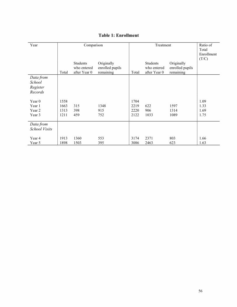
Table 1: Enrollment
Year Comparison Treatment Ratio of
Total Enrollment (T/C)
Total
Students who entered after Year 0
Originally enrolled pupils remaining Total
Students who entered after Year 0
Originally enrolled pupils remaining
Data from School Register Records
Year 0 1558 1704 1.09 Year 1 1663 315 1348 2219 622 1597 1.33 Year 2 1313 398 915 2220 906 1314 1.69 Year 3 1211 459 752 2122 1033 1089 1.75 Data from School Visits
Year 4 1913 1360 553 3174 2371 803 1.66 Year 5 1898 1503 395 3086 2463 623 1.63
56
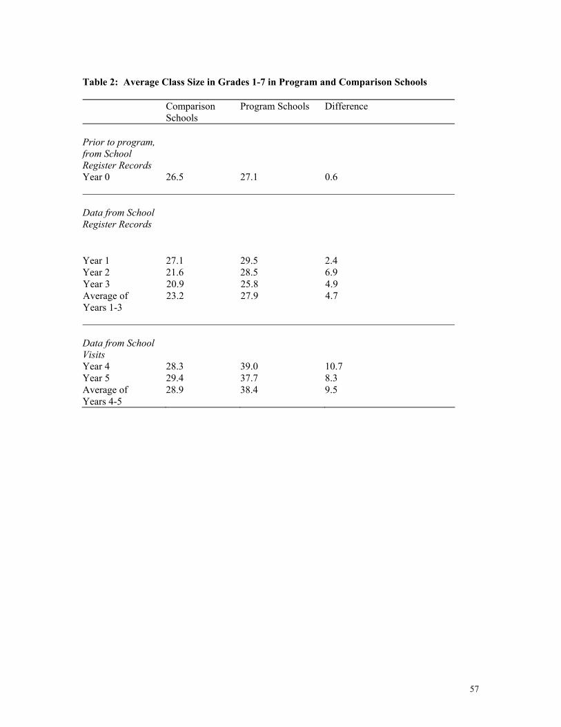
Table 2: Average Class Size in Grades 1-7 in Program and Comparison Schools Comparison
Schools Program Schools Difference
Prior to program, from School Register Records
Year 0 26.5 27.1 0.6 Data from School Register Records
Year 1 27.1 29.5 2.4 Year 2 21.6 28.5 6.9 Year 3 20.9 25.8 Average of Years 1-3
23.2 27.9 4.9 4.7
Data from School Visits
Year 4 28.3 39.0 10.7 Year 5 29.4 37.7 8.3 Average of Years 4-5
28.9 38.4 9.5
57
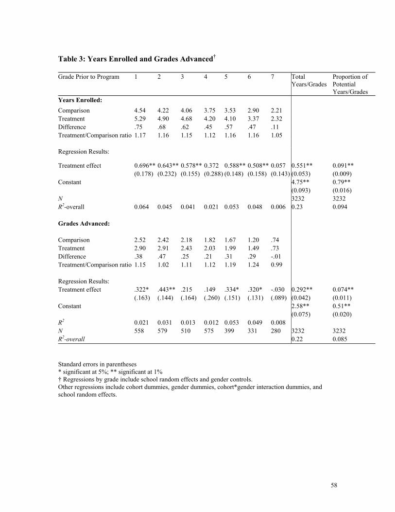
Table 3: Years Enrolled and Grades Advanced†
Grade Prior to Program 1 2 3 4 5 6 7 Total
Years/Grades Proportion of Potential Years/Grades
Years Enrolled: Comparison 4.54 4.22 4.06 3.75 3.53 2.90 2.21 Treatment 5.29 4.90 4.68 4.20 4.10 3.37 2.32 Difference .75 .68 .62 .45 .57 .47 .11 Treatment/Comparison ratio 1.17 1.16 1.15 1.12 1.16 1.16 1.05 Regression Results:
Treatment effect 0.696** 0.643** 0.578** 0.372 0.588** 0.508** 0.057 0.551** 0.091** (0.178) (0.232) (0.155) (0.288) (0.148) (0.158) (0.143) (0.053) (0.009) Constant 4.75** 0.79** (0.093) (0.016) N 3232 3232 R2-overall 0.064 0.045 0.041 0.021 0.053 0.048 0.006 0.23 0.094 Grades Advanced: Comparison 2.52 2.42 2.18 1.82 1.67 1.20 .74 Treatment 2.90 2.91 2.43 2.03 1.99 1.49 .73 Difference .38 .47 .25 .21 .31 .29 -.01 Treatment/Comparison ratio 1.15 1.02 1.11 1.12 1.19 1.24 0.99 Regression Results: Treatment effect .322* .443** .215 .149 .334* .320* -.030 0.292** 0.074** (.163) (.144) (.164) (.260) (.151) (.131) (.089) (0.042) (0.011) Constant 2.58** 0.51** (0.075) (0.020) R2 0.021 0.031 0.013 0.012 0.053 0.049 0.008 N 558 579 510 575 399 331 280 3232 3232 R2-overall 0.22 0.085 Standard errors in parentheses * significant at 5%; ** significant at 1% † Regressions by grade include school random effects and gender controls. Other regressions include cohort dummies, gender dummies, cohort*gender interaction dummies, and school random effects.
58
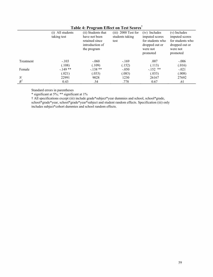
Table 4: Program Effect on Test Scores†
(i) All students taking test
(ii) Students that have not been retained since introduction of the program
(iii) 2000 Test for students taking test
(iv) Includes imputed scores for students who dropped out or were not promoted
(v) Includes imputed scores for students who dropped out or were not promoted
Treatment
-.103 (.108)
-.060 (.109)
-.169 (.152)
.007 (.113)
-.006 (.016)
Female
-.149 ** (.021)
-.138 ** (.033)
-.050 (.083)
-.152 ** (.033)
-.021 (.008)
N 22991 9028 1230 26167 27692 R2 0.43 .54 .778 0.67 .61
Standard errors in parentheses * significant at 5%; ** significant at 1% † All specifications except (iii) include grade*subject*year dummies and school, school*grade, school*grade*year, school*grade*year*subject and student random effects. Specification (iii) only includes subject*cohort dummies and school random effects.
59
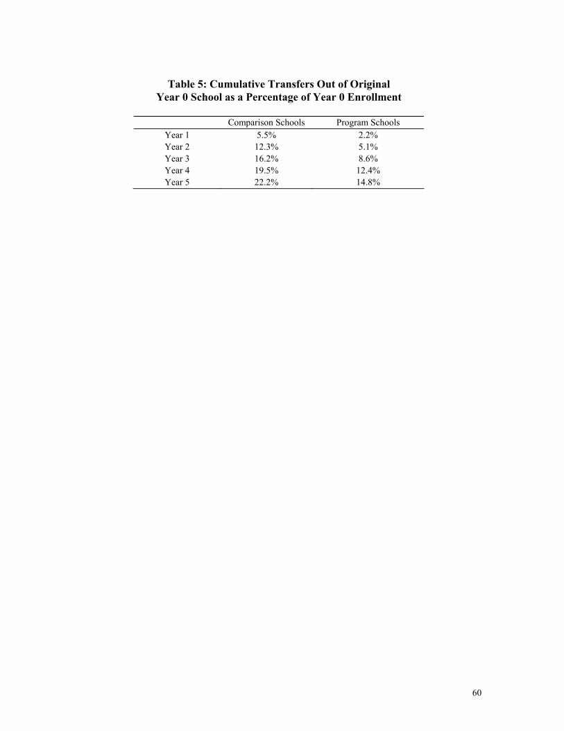
Table 5: Cumulative Transfers Out of Original
Year 0 School as a Percentage of Year 0 Enrollment
Comparison Schools Program Schools Year 1 5.5% 2.2% Year 2 12.3% 5.1% Year 3 16.2% 8.6% Year 4 19.5% 12.4% Year 5 22.2% 14.8%
60
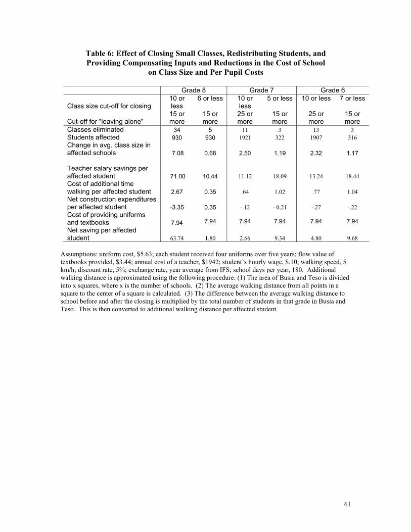
Table 6: Effect of Closing Small Classes, Redistributing Students, and Providing Compensating Inputs and Reductions in the Cost of School
on Class Size and Per Pupil Costs
Grade 8 Grade 7 Grade 6
Class size cut-off for closing 10 or less
6 or less 10 or less
5 or less 10 or less 7 or less
Cut-off for "leaving alone" 15 or more
15 or more
25 or more
15 or more
25 or more
15 or more
Classes eliminated 34 5 11 3 13 3 Students affected 930 930 1921 322 1907 316 Change in avg. class size in affected schools 7.08 0.68 2.50 1.19 2.32 1.17 Teacher salary savings per affected student 71.00 10.44 11.12 18.09 13.24 18.44 Cost of additional time walking per affected student 2.67 0.35 .64 1.02 .77 1.04 Net construction expenditures per affected student -3.35 0.35 -.12 - 0.21 -.27 -.22 Cost of providing uniforms and textbooks 7.94
7.94
7.94
7.94
7.94
7.94
Net saving per affected student 63.74 1.80 2.66 9.34 4.80 9.68
Assumptions: uniform cost, $5.63; each student received four uniforms over five years; flow value of textbooks provided, $3.44; annual cost of a teacher, $1942; student’s hourly wage, $.10; walking speed, 5 km/h; discount rate, 5%; exchange rate, year average from IFS; school days per year, 180. Additional walking distance is approximated using the following procedure: (1) The area of Busia and Teso is divided into x squares, where x is the number of schools. (2) The average walking distance from all points in a square to the center of a square is calculated. (3) The difference between the average walking distance to school before and after the closing is multiplied by the total number of students in that grade in Busia and Teso. This is then converted to additional walking distance per affected student.
61
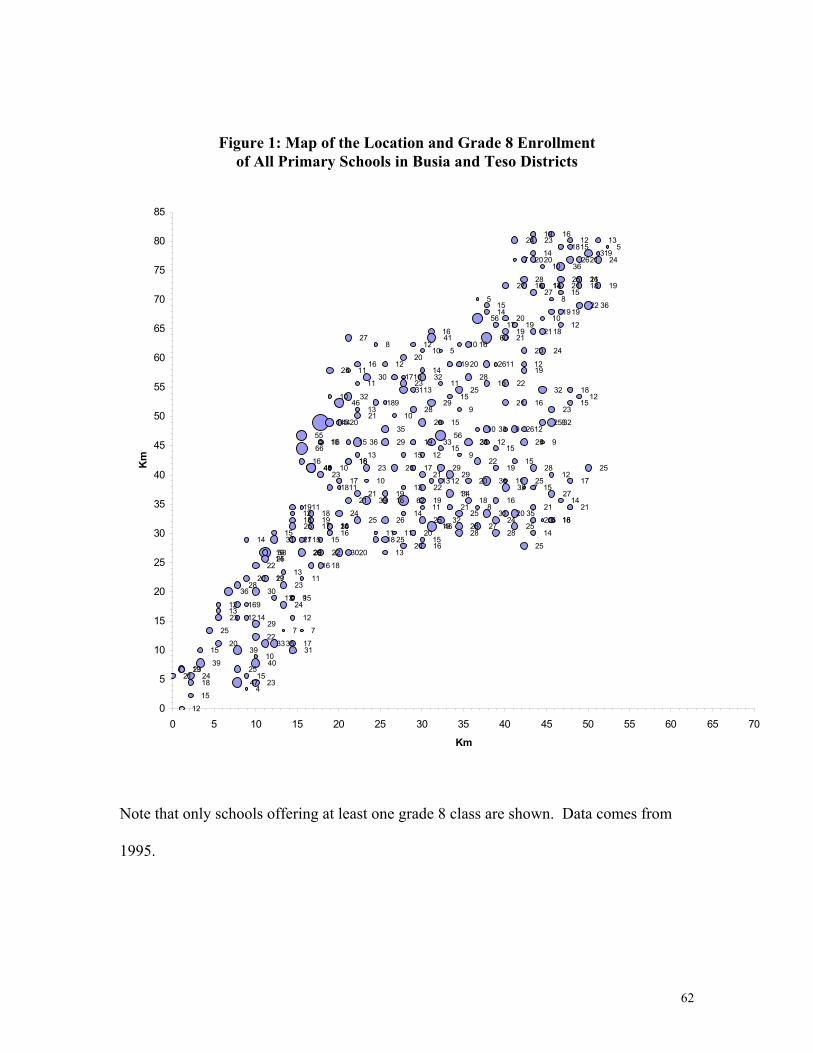
Figure 1: Map of the Location and Grade 8 Enrollment of All Primary Schools in Busia and Teso Districts
18
2114
12
5
17
26
28
12
35
15
20 16
8
28
20
12
7
12
58
10
13
23
24
15
16
2420
13
36
15
16
19
25
21
6
21
20
14
30
20
19
19
16
13
18
12
9
12
20
8
10
19
28
13
4
21
7
62
25
27
1219
28
14
17
19
10
22
9
311815
9
23
1010
39
15
18
19
1911
18
16
13
16
17
14
29
1321
20
15
12
3915
21 24
40
18 4715
20
23
23
3133
25
19
27
25
2724
14
16
25
1512
34
20 28
16
11
20 3532
32
25
25
19
25
36
31
17
13
12
25
28
11
20
11
264618
15936
11
25
9
15
2313
18 24
29
11
18
22
7
25
17
2117
12
23
24
2829
16
31
20
13
161514
22
30
23
36
21
23
2211
1639
292923
1618
15
2625
15
19
25
9
32
15
15
2331
26
18
9
1621
33
33
29
56
15
8
25
32
6616
16
10
48
55
27
22
28
19
15
36
1916
25
12
26
1314
17
27
16
10
15
19
21
7
27
2121
24
2116
5
1956
23
19
20
18
1220
1046 9
1120
20
32
25
30
13
31
48
3229
60
1014
19 11
22
41
16
2144
10
128
11
18
16
35
2111
18
11
12
22
10
15
17
5
14
10
12
14
14
115
25
0
5
10
15
20
25
30
35
40
45
50
55
60
65
70
75
80
85
0 5 10 15 20 25 30 35 40 45 50 55 60 65 70
Km
Km
Note that only schools offering at least one grade 8 class are shown. Data comes from
1995.
62
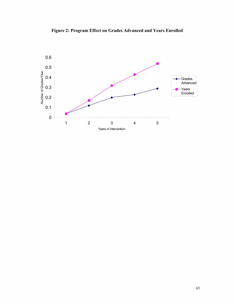
Figure 2: Program Effect on Grades Advanced and Years Enrolled
0
0.1
0.2
0.3
0.4
0.5
0.6
1 2 3 4 5Years of Intervention
Num
ber o
f Gra
des/
Yea
rs
GradesAdvanced
YearsEnrolled
63