Benedetta MennucciDipartimento di Chimica e Chimica Industriale

Web: http://benedetta.dcci.unipi.it Email: bene@dcci.unipi.it

An introduction to continuum solvationmodels for quantum chemistry

An introduction to continuum solvationmodels for quantum chemistry

IMA Thematic Year on Mathematics and Chemistry:

SolvationTutorial:

Theories of Solvation Within Quantum

Chemistry

December 7, 2008

InteractionsInteractions

As first step, any theoretical model requires the definition of the interactions acting among particles.

Isolated moleculeelectrons and nuclei to form the molecule

Liquidsmolecules to form the solution

– Bulk polarization– Site binding or specific solvation– Preferential hydration– …

Discrete (or miscroscopic description)

1. Classical simulations (Monte Carlo, Molecular Dynamics)

Classical MM (force fields) for all molecules.

2. QM/MM

QM for a small part of the system and MM for all the rest.

Modeling interactionsModeling interactions

Modeling interactionsModeling interactions

Explicit consideration of a large number of trajectories (MD) or of MC steps

Time consumingDifficult to extend to QM descriptions

How to achieve a statistically correct description?

How to deal with the large dimension of the systems?

Force Fields

Parameterization; Generally non-polarizable potentials; Generally Periodic boundaries; Problems with long-range interactions

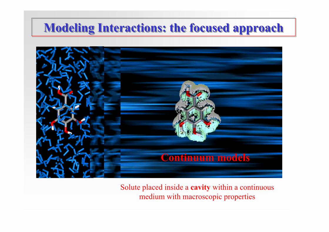
Continuum models

Solute placed inside a cavity within a continuousmedium with macroscopic properties

Modeling Interactions: the focused approachModeling Interactions: the focused approach

Continuum models

How to deal with the large dimension of the systems?

The solvent molecules disappear and they are substituted by a continuous dielectric that surrounds a

cavity containing the solute molecule

No need to introduce force fieldsPolarizable dielectricComplete inclusion of long-range interactions

Implicitly accounted for using the macroscopic properties of the continuum (the dielectric

permittivity, the refractive index, etc)

Computationally cheapStraightforward to extend to QM descriptions

How to achieve a statistically

correct description?

Modeling Interactions: the focused approachModeling Interactions: the focused approach

Continuum Models

A short history

• Electrostatic component of the free energy of solvation for a charge (q) in a spherical cavity of radius a inside the solvent:

2 112elecqGa ε

⎛ ⎞Δ = − −⎜ ⎟⎝ ⎠

Born (1920)Born (1920)Born (1920)

Dielectric permittivityof the solvent

ΔGelec

Cavityradius

work done to transfer the ion from vacuum to the medium.

This is the difference in work to charge the ion in the two environments.

Several charges:

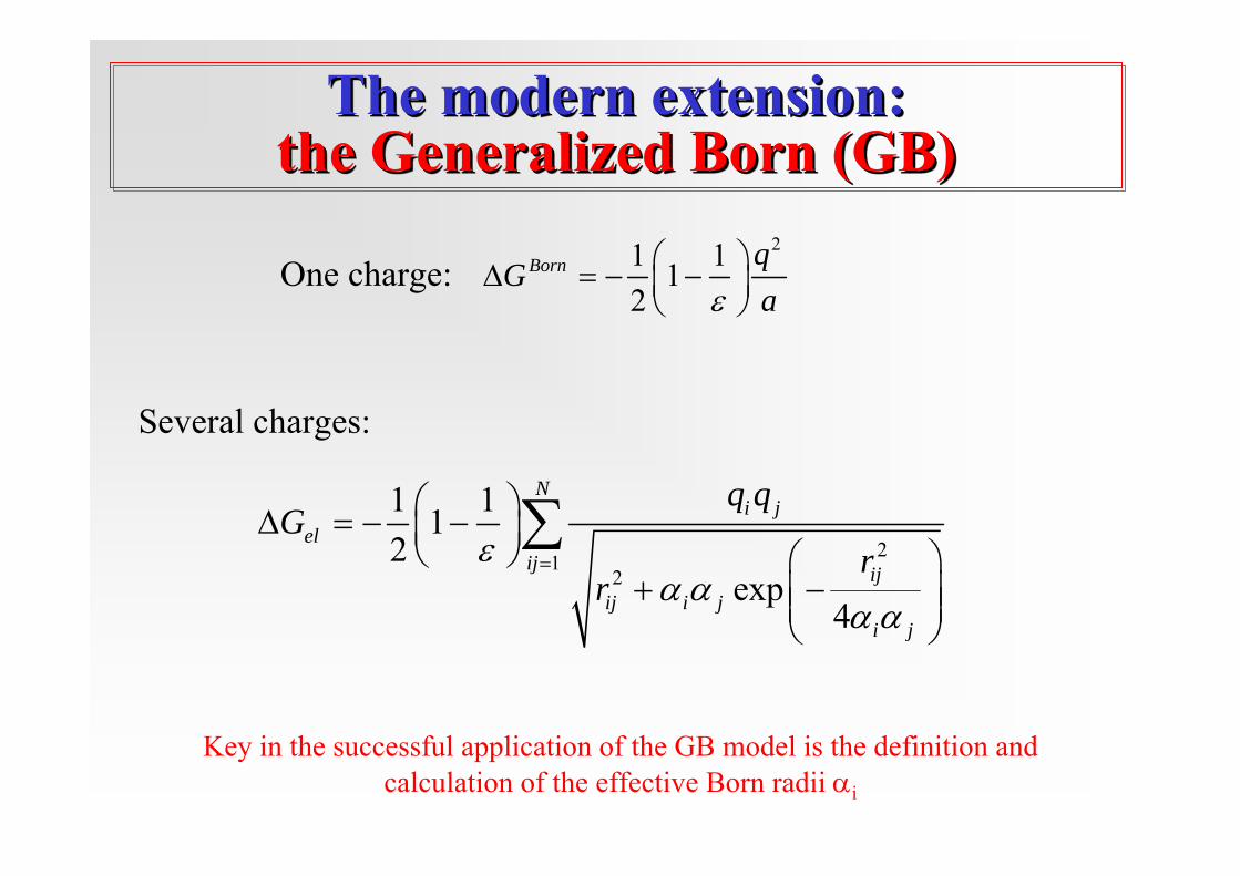
The modern extension: the Generalized Born (GB)

The modern extension: The modern extension: the Generalized Born (GB)the Generalized Born (GB)

Key in the successful application of the GB model is the definition and calculation of the effective Born radii αi

212

1 112

exp4

Ni j

elij ij

ij i ji j

q qG

rr

εα α

α α

=

⎛ ⎞Δ = − −⎜ ⎟⎝ ⎠ ⎛ ⎞

+ −⎜ ⎟⎜ ⎟⎝ ⎠

∑

21 112

Born qG

aε⎛ ⎞Δ = − −⎜ ⎟⎝ ⎠

One charge:

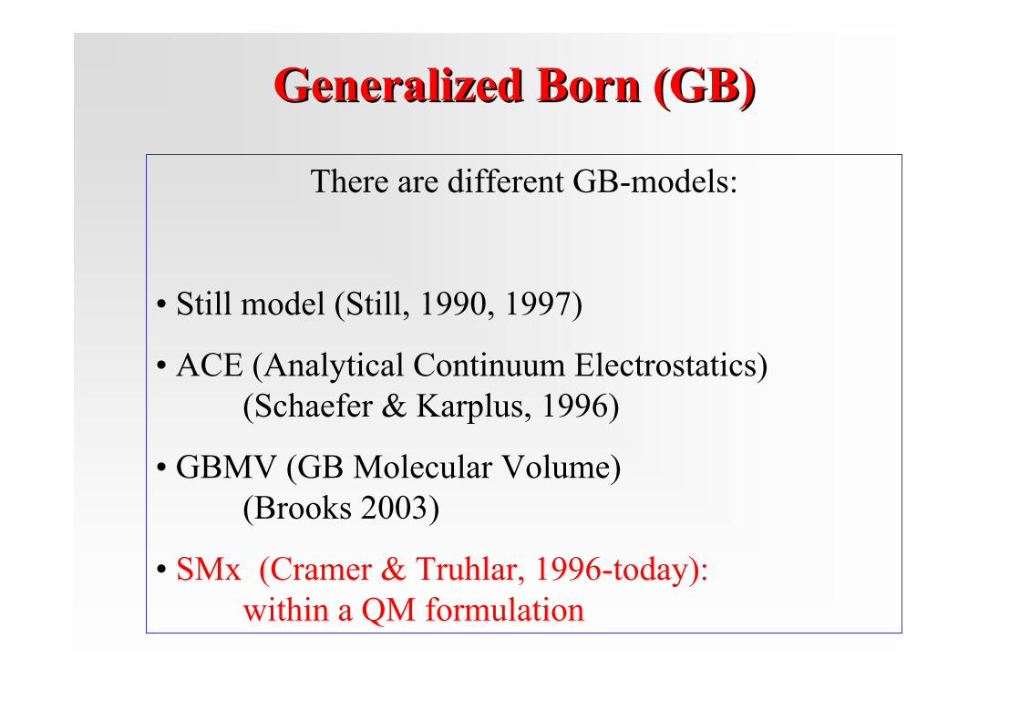
There are different GB-models:

• Still model (Still, 1990, 1997)

• ACE (Analytical Continuum Electrostatics) (Schaefer & Karplus, 1996)

• GBMV (GB Molecular Volume)(Brooks 2003)

• SMx (Cramer & Truhlar, 1996-today): within a QM formulation

Generalized Born (GB)Generalized Born (GB)Generalized Born (GB)

Onsager (1936)OnsagerOnsager (1936)(1936)

μ

ε

When a molecule with a permanent dipole μμ is surrounded by other particles, the electric field produced by the permanent dipole polarizes its environment.

Dipole moments are induced in the surrounding molecules, and if they have a permanent dipole moment their orientation is influenced too.

The polarization of the dielectric gives rise to a field at the dipole (the reaction field R)

fR μ=reaction field

factor

Simple model:

an ideal dipole in a center of a spherical cavity inside continuum dielectric

The Onsager ModelThe The OnsagerOnsager ModelModelA spherical cavity with radius a in a continuous dielectric of permittivity ε.

The point dipole with moment μμ is situated in the center of the cavity.

μ

ε

a 3

1 2( -1)2 1

R fa

εμ με

= =+

Work done in assembling the chargedistribution μ within the dielectric

Electrostatic free energy of solvation

( )( )

2

3

12 1elecG

aε με−

Δ = −+

12

R μ⋅

Reaction field of the solvent

The modern extension: the multipole expansion (MPE)

The modern extension: The modern extension: the the multipolemultipole expansion (MPE)expansion (MPE)

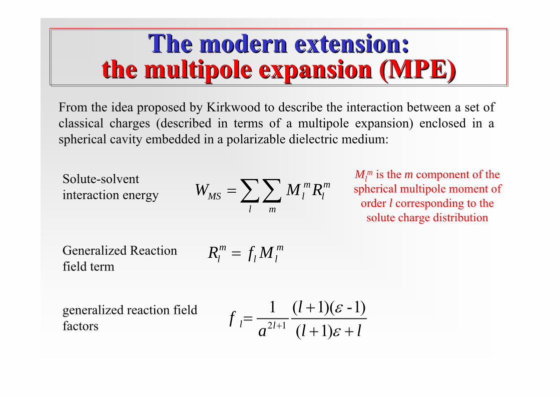
From the idea proposed by Kirkwood to describe the interaction between a set of classical charges (described in terms of a multipole expansion) enclosed in a spherical cavity embedded in a polarizable dielectric medium:

Mlm is the m component of the

spherical multipole moment of order l corresponding to the solute charge distribution

Solute-solvent interaction energy

Generalized Reaction field term

generalized reaction fieldfactors

m ml l lR f M=

2 1

1 ( 1)( -1)( 1)l l

lfa l l

εε+

+=

+ +

m mMS l l

l m

W M R= ∑∑

There are different MPE-models:

• Nancy model (Rivail & coworkers., 1973-today)

• Copenhagen model (Mikkelsen & coworkers, 1988-today)

Both have been formulated within a QM framework

Multipole extension (MPE)MultipoleMultipole extension (MPE)extension (MPE)

Limits of GB and MPE models for quantum chemistry

Limits of GB and MPE models for quantum chemistry

a) molecular cavity:

use of effective Born Radii

use of a sphere (or an ellipse)

b) description of the solute charge distribution:

use of a set of atom-centered partial charges

use of a dipole (or a multipole expansion)

The molecular cavityThe molecular cavityThe molecular cavity

A realistic cavity should be modeled on the 3D structure of the solute

Standard method: overlapping spheres centered

on the nuclei forming the molecular system

DNA fragment

3. Solvent excluded Surface (SES): is the surface traced out by the inward-facing part of the probe sphere as it rolls on the VDW surface.

1. van der Waals Surface (VWS):is constructed from the overlapping vdW spheres of the atoms

2. Solvent Accessible Surface (SAS): is the surface traced by the center of the probe sphere as it rolls on the VDW surface.

Molecular cavity: not a unique definitionMolecular cavity: not a unique definitionMolecular cavity: not a unique definition

Connolly (1983):

Alternative approach: GePol (Pascual-Ahuir 1994)

Reentrant (concave) surface

Convex surface

Spheres centered on solute atoms

Electrostatic interactions:Solvent-excluded surface (SES)

Electrostatic interactions:Solvent-excluded surface (SES)

Probe sphere representingthe solvent

Added spherenot centered

on atoms

Easier toimplement!

The Poisson equationThe Poisson equation

Mathematical problem:

Physical Problem:A charge density ρM inside a cavity (C) within a continuum dielectric described by its permittivity ε ρM n

2 4 MV πρ−∇ =2 0Vε− ∇ =

Jump conditionInside C

Outside C

in outV V=in out

V n V nε⎡ ⎤ ⎡ ⎤∇ ⋅ = ∇ ⋅⎣ ⎦ ⎣ ⎦

The electrostatic potential V has to satisfy the differential equations inside and outside the cavity (together with the proper boundary conditions)

+

( )( ) ( ) 4 ( )Mr V r rε πρ−∇ ⋅ ∇ =

0V → At infinity

ε > 1ε =1

A possible solution: the Apparent Surface Charge (ASC)

A possible solution: the Apparent Surface Charge (ASC)

The reaction potential is defined by introducing an apparent surface charge

density (σ) on the cavity

ε

ρMn

Which electrostatic potential V ?

V is the sum of the electrostatic potentialVM generated by the charge distribution ρMand of the reaction potential VR generatedby the polarization of the dielectricmedium:

Which form for the reaction potential VR ?

2( )( ) ( )RsV r V r d s

r sσσ

Γ⇒ =

−∫

( ) ( ) ( )M RV r V r V r= +

ASC: different formulationsASC: different formulations

2( ) ( ( ))RV r V r ds

s srσσ

Γ⇒ =

−∫

Which definition for σ?

The family of PolarizableContinum Models (PCM)

( ) ( )( ) ( ) ( ) ( )R M MsE r E r dr r ds V s ds

rs

sσσρ σ

Γ Γ⇒ = =

−∫ ∫ ∫

Reaction potential:

Interaction energy:

For dielectrics with a constant isotropic permittivity, the solvent polarizationvector is (linear response approximation):

ε > 1

n

ε =1

The original formulation: DPCM (1981)The original formulation: DPCM (1981)

At the boundary of two regions i and j, there is an apparent surface chargedistribution given by

Taking into account that :εi = 1 (inside the cavity there is no dielectric) εj> 1 (outside the cavity there is the solvent)

14

P Eεπ−

=

( )ij i j ijP P nσ = − − ⋅

( )1 14 4

DPCMME n E E nσ

ε εσπε πε− −

= − ⋅ = − + ⋅

The Conductor-like formulation: COSMO (CPCM)The Conductor-like formulation: COSMO (CPCM)A conductor (infinite permittivity, ε =∞) instead of a dielectric: a new condition on the total potential

( ) ( ) 0M RV r V r+ = the potential on a cavity inside the conductor is null

A much easier condition to satisfy:

ˆ 0CMV Sσ+ =

We recover the true dielectric behavior by scaling the conductor charges using the real (finite) dielectric constant:

1CPCM Cεσ σε−

=

( )( ) ( )|

ˆ|

CC

RsV r V r ds

r sSσ

σ σ→ = =−∫ Integral operator S

1ˆCMS Vσ −= − Conductor

apparent charge

The conductor-like model is the DPCM limit for ε→∞i.e. very polar solvents: practically, it is a goodapproximation for ε ≥ 5

2 4in ML V πρ= −∇ =

( )ˆ ( ) ( , ) ( )k kS f x x f yG y y dΓ

= ∫

( )ˆ ( ) ( , ) ( ) ( )

,

k kkD f x x y n y f y dy

k out in

GεΓ

= ∇ ⋅⎡ ⎤⎣ ⎦

=∫

( ) ( )*ˆ ˆ ˆˆ ˆ ˆ ˆ2 2inout in outA I D S S I Dπ π= − ⋅ + ⋅ +

( ) ˆˆ ˆ2M

Mout M out

Vb I D V Snρ π ∂⎡ ⎤= − +⎢ ⎥∂⎣ ⎦

TheThe apparent surface chargeapparent surface charge is obtained in terms of integral operators (Sk, Dk) defined on the cavity surface (Γ) and of the solute potential (VM) on the same surface

Green functions of Lin and Lout partial operators:(for simplicity’s sake we drop the vector symbol)

1( , )| |inG x yx y

=−

1( , )outG x yx yε

=−

ˆM

IEFPCMA bρσ = −

2 0outL Vε= − ∇ =

in outV V=

M M

in out

V Vn n

ε∂ ∂⎡ ⎤ ⎡ ⎤=⎢ ⎥ ⎢ ⎥∂ ∂⎣ ⎦ ⎣ ⎦

Integral Equation Formalism: Integral Equation Formalism: IEFIEF (1997)(1997)

ε||

ε⊥

ε⊥

Anisotropic dielectric:

It can be applied to different environments: we have only to change the Green function Gout (outside the cavity) according to the proper Lout operator

1

z-z0

2

For example: a nematic liquid crystal

A diffuse interface between gas/liquid or liquid/liquid(numerical solution):

01 2 1 2( ) tanh2 2

z zzD

ε ε ε εε−+ − ⎛ ⎞= + ⎜ ⎟

⎝ ⎠

⎟⎟⎟

⎠

⎞

⎜⎜⎜

⎝

⎛=

zz

yy

xx

ε000ε000ε

εTensorialpermittivity

... and metal surfaces, metal spheres …

Ionic solutions: Linearized PB

Integral Equation Formalism: Integral Equation Formalism: IEFIEF (1997)(1997)

It contains as sub-cases both DPCM and COSMO

*1 ˆ ˆ21

DPCM Min

VI Dn

επ σε

⎡ + ⎤ ∂⎛ ⎞ − =⎜ ⎟⎢ ⎥− ∂⎝ ⎠⎣ ⎦

( )1 ˆˆ ˆ ˆ ˆ2 21

IEFPCMin in in MI D S I D Vεπ σ π

ε⎡ + ⎤⎛ ⎞ − = − −⎜ ⎟⎢ ⎥−⎝ ⎠⎣ ⎦

ˆ Cin MS Vσ = −

( )ˆ ˆ2 0Min M in

VI D V Sn

π ∂− + =

∂ ε → ∞

DPCM COSMO

An efficient reformulation: An efficient reformulation: IEFIEF--PCMPCM ((SS(V)PESS(V)PE))

The numerical solution: a boundary element method

The numerical solution: a boundary element method

4. Discretization of the apparent surface charge σ into N point-like charges q

2. Partition of the cavity surface into N finite elements (tesserae) (Boundary Element Method, BEM)

3. Reformulation of the integral operators into matrices

1. Construction of the molecular cavity in terms of interlocking spheres(centered on the solute atoms) using the GEPOL algorithm

*1 ˆ ˆ21

DPCMin MI D E nεπ σ

ε⎡ + ⎤⎛ ⎞ − = − ⋅⎜ ⎟⎢ ⎥−⎝ ⎠⎣ ⎦

( )1 ˆˆ ˆ ˆ ˆ2 21

IEFin in in MI D S I D Vεπ σ π

ε⎡ + ⎤⎛ ⎞ − = − −⎜ ⎟⎢ ⎥−⎝ ⎠⎣ ⎦

ˆ Cin MS Vσ = −

Discretization of the surface charge: the P0 approximation

Discretization of the surface charge: the P0 approximation

( )isσ constant on eachelement of area ai

( )i i iq a sσ=

ˆ square matrix ( ) S N N⇒ × S

ˆ square matrix ( ) D N N⇒ × D

si

DPCM COSMO

IEFPCM

ˆ ˆ( )

M

M

E nT R

Vε σ

⎧ ⋅⎪= − ⎨⎪⎩

N finite elements

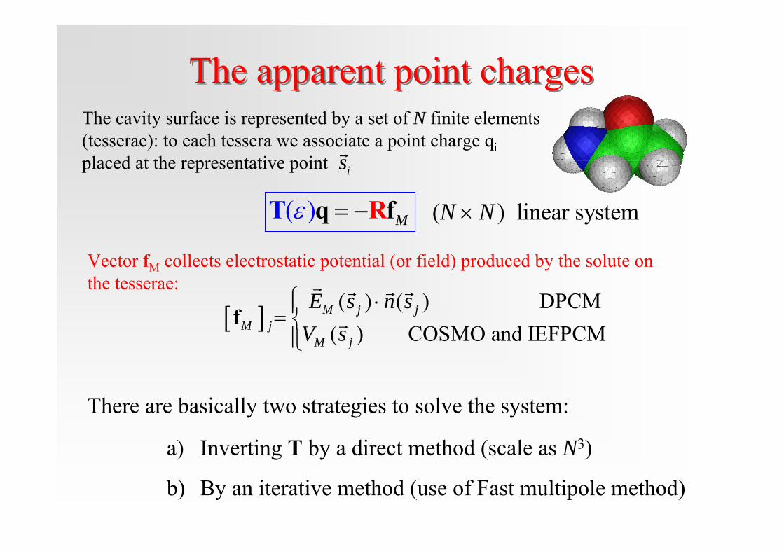
The apparent point chargesThe apparent point charges

[ ] ( ) ( ) DPCM( ) COSMO and IEFPCM

M j jM j

M j

E s n sV s

⎧ ⋅⎪= ⎨⎪⎩

f

Vector fM collects electrostatic potential (or field) produced by the solute on the tesserae:

The cavity surface is represented by a set of N finite elements(tesserae): to each tessera we associate a point charge qiplaced at the representative point is

( ) Mε = −T Rq f ( ) linear systemN N×

There are basically two strategies to solve the system:

a) Inverting T by a direct method (scale as N3)

b) By an iterative method (use of Fast multipole method)

The QM problemThe QM problem

The SelfThe Self--Consistent Reaction Field (SCRF) methodConsistent Reaction Field (SCRF) method

QM Theory of continuum solvationQM Theory of continuum solvation

Solute-solvent electrostatic interactions

Proper QM operator defined on the cavity surface: it depends on the solute charge density (ρ)

0

0

eff

s

H H→

Ψ → Ψ

Isolated system

Solvated system Effective

Hamiltonian

Polarized wavefunction

0eff s R s s sH H V E⎡ ⎤Ψ = + Ψ = Ψ⎣ ⎦

( ) ( ; ) ( )Rk k

kV q s V sρ ρ= ∑

Self-Consistent Reaction Field (SCRF)Mutual polarization of solute and solvent

charge distributions

ˆ ˆk k

k

R qV V= ∑

M= −Tq RV

1( ) ˆ N ki i

Ki KM i

i

V ZV Vr R s

ss

= Ψ Ψ + = − Ψ Ψ +− −∑

Effective QM equations: a nonlinear problemEffective QM equations: a nonlinear problem

The solvent operator depends on the wavefunction it contributse to determine

An iterative scheme is requiredIt can be solved together with the standard self-consistent-field problem

Solute electrostatic potential on the surface cavity:

Solvent reactionpotential operator

0 ˆˆ ˆff sRe VH H E⎡ ⎤Ψ = + Ψ = Ψ⎣ ⎦Effective Schrodingerequation for the solute

ASC

IEFPCM

EffectiveFock operator ˆˆ ˆˆ ˆ RReff hF Xh G= + + +

The self consistent reaction fieldThe self consistent reaction field

ˆ ˆneh T V= +Mono-electronic ˆ ˆR N

i ii

h q V= ∑N N

M= −Tq RVApparent charges induced by the solute nuclear potential: they do not depend on the wavefunction.

They do not change in the SCF cycle

ˆ ˆ ˆG J K= −Bi-electronic ˆ ˆR eli i

i

X q V= ∑el el

M= −Tq RV

ˆ( )elM i iV s V= − Ψ Ψ

Apparent charges induced by the solute electrons: they depend on the wavefunction.

They change at each iteration of the SCF cycle

( )N kM i

K K i

ZV sR s

=−∑

Within a QM description of the solute electronic charge: the electronic tail of the solute necessarily spreads outside the cavity (escaped or outlying charge)

ε

(out)

(in) n

Δ 4Δ 0

MVV

πρ=− =

(in)(out)

Boundary conditions

The PCM theory has been formulated for an ideal charge density completely inside the cavity

The reaction field should be expressed by two apparent charge distributions:

14

E nεσπε−

= − ⋅1 out

Mεβ ρ

ε−

= −

On the cavity surface In the outside volume

QM-ASC Theory of Solvation: the oulyingcharge effect

QM-ASC Theory of Solvation: the oulyingcharge effect

The outlying charge effectThe outlying charge effect

β is easily computed once ρ is known, but its contribution to the reaction field raisessevere problems (involves an integration over the whole space outside the cavity !).

The electrostatic interaction between solute and solvent (solvent reaction field) should becomputed by a double integration

Which is the effect of neglecting β ?

Gauss Theorem

14

4V V

ds E nds

E nds Edv dv

εσπε

π ρ

Γ Γ

Γ

−= − ⋅

⋅ = ∇ ⋅ =

∫ ∫∫ ∫ ∫

1calci M

i

q Q Qεε−

= = −∑

In the real word:1calc

MQ Qεε−

≠ −

In the ideal world:

A solution for the outlying charge effectA solution for the outlying charge effectTo have a more correct description of the solvent polarization we have

to find a way to include the effects of the volume apparent charge β

These effects can be approximated by an additional surface charge.

But: ( ( ) )' IEFPCM SS V PEσ σ⇔

1 ˆ ˆ ˆ ˆ2 * ' 21 MS SD I D Vεπ σ π

ε⎡ + ⎤⎛ ⎞ ⎡ ⎤− = − −⎜ ⎟⎢ ⎥ ⎣ ⎦−⎝ ⎠⎣ ⎦

'σ σ α= +

IEFPCM (or SS(V)PE) charges produce inside the

cavity an exact reactionpotential!!

α can be defined so to generate inside the cavity the same electrostaticpotential as that due to β:

S Vβα =

*1 ˆ ˆ21 MI D E nβ

επ σε +

⎡ + ⎤⎛ ⎞ − = − ⋅⎜ ⎟⎢ ⎥−⎝ ⎠⎣ ⎦

Beyond the electrostatic approachBeyond the electrostatic approach

The free energy of solvationThe free energy of solvation

ΔGsol = ΔGelec + ΔGdisp-rep + ΔGcav

Electrostaticfree energy

Dispersion & repulsion free

energy

Cavitation free energy: work required to form the

cavity

0 0 0 012elec

RH V HG = Ψ Ψ + Ψ Ψ − Ψ ΨΔ

Cavitation: Steric InteractionsCavitation: Steric InteractionsMechanical forces: no need of QM descriptionsRepresentation in terms of rigid classical spherical bodiesObjective: work required to build the molecular cavity

A possible approach: Scaled Particle Theory

• selection of a spherical particle A

• definition of a pairwise additive potential: VAB

• evaluation of the work (Gcav(A)) required to exclude centers of other particles from the spherical region occupied by A

A

Generalization to a multi-sphere cavity:

2 ( )4π

spherescav cavi

ii i

SG G RR

= ∑Exposed surface of sphere i

Single sphere contribution

Dispersion & Repulsion : the semiclassical approachDispersion & Repulsion : the semiclassical approach

( )

( )( )n

dis rep dis rep dis rep msms ms ms nm M s S n ms

dV V r Vr

− − −

∈ ∈= ∑ ∑ ⇔ = ∑

In a Molecular Mechanics framework: atom-atom pairwise potential between solute (M) and solvent (S)

solvent solute tesseraedis rep dis rep

s s i ms is m i

G N a A nρ− −= ⋅∑ ∑ ∑

But…..we cannot take into account repulsion and dispersion effects on the solute electronic distribution but only on the solvation free energy.

In a continuum framework:a discrete sum over the tesserae of the cavity surface:

( )dis rep disp repms ms ms msA V r g− −∇ ⋅ =

gms =correlation functionapproximated as a step function(0 inside the cavity, 1 outside)

Nonelectroctatic terms: a unified approach

Nonelectroctatic terms: a unified approach

It is based on the use of a linear relationship with the solvent-accessible surface (SAS) of the solute

where Sm denotes the contribution of atom m to the surfaceof the cavity, and σm is the surface tension of atom m

solutedis rep

m mm

G Sσ− = ∑

But…..we cannot take into account repulsion and dispersion effects on the solute electronic distribution but only on the solvation free energy.

Generalizing the QM theory of intermolecular forces

Two interacting molecules

Depend on the portion of solute electronic density outside the cavity

Depend on the solute transition potential and the corresponding solvent surface charges

Solute + a continuous solvent

Repulsion & dispersione: the QM approachRepulsion & dispersione: the QM approach

Repulsion forces: depend on the overlap of the charge distributions of the two molecules.

Dispersion forces: depend on the interaction of the transition densities of the two molecules

3repulsion en (e gy )rout

rep Mr V

k r d rρ∈

→ ∫ It is proportional to the portion of solute electronic charge outside the cavity

0 00

dispersion energy ( ) ( ) Md K

Kis KV s s dsk σ

≠ Σ

→ ∑∫It is proportional to the interaction

between the solute transition potential between ground and excited states (K)and the corresponding solvent surface

charges σ0K

0 R rep disH V V V E⎡ ⎤+ + + Ψ = Ψ⎣ ⎦The resulting wavefunction is now affected also by repulsion and

dispersion solute-solvent interactions

It is now possible to define QM operators which represent the solute-solvent repulsion and dispersion interactions

Repulsion & dispersione: the QM approachRepulsion & dispersione: the QM approach

ConclusionsConclusions

…but they have to be:

1. general (not limited in the form of the cavity or in the description of the solute)

2. extensible to treat different environments (not only homogeneous and isotropic liquids)

3. coupled to different QM methods (for ground and excited states), as well as to their extensions to derivative approaches(for geometry optimizations and response properties)

Continuum models may represent a very effective approach to study solvent effects on energies/properties and reactivity of

solvated systems.

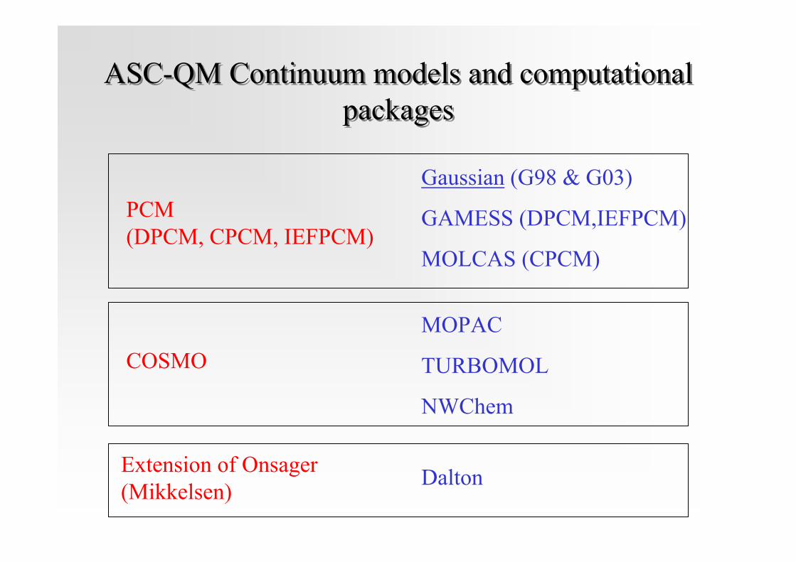
ASC-QM Continuum models and computationalpackages

ASC-QM Continuum models and computationalpackages

PCM (DPCM, CPCM, IEFPCM)

Gaussian (G98 & G03)

GAMESS (DPCM,IEFPCM)

MOLCAS (CPCM)

COSMOMOPAC

TURBOMOL

NWChem

Extension of Onsager(Mikkelsen) Dalton

LiteratureLiteratureGeneral reviews about QM continuum models

J. Tomasi, M. Persico, Chem. Rev., (1994) 94, 2027C. J. Cramer, D. G. Truhlar, Chem. Rev. (1999) 99, 2161J. Tomasi, B. Mennucci, R. Cammi, Chem. Rev. (2005) 105, 2999B. Mennucci, & R. Cammi (Eds.) “Continuum solvation models in Chemical Physics: from theory to applications”, Wiley (2007)

Miertus, S.; Scrocco, E.; Tomasi, J. Chem. Phys. 1981, 55, 117.

Klamt, A.; Schuurmann, G. J. Chem. Soc., Perkin Trans. 1993, 2, 799.

Barone, V.; Cossi, M. J. Phys. Chem. A 1998, 102, 1995

Cancès, E.; Mennucci, B.; Tomasi, J. J. Chem. Phys. 1997, 107 3032

DPCM

COSMO

CPCM

IEFPCM

Chipman D.M., J. Chem. Phys. 2000, 112, 5558.SS(V)PE

ASC

mod

els