Embed Size (px)
Citation preview
Deceiving Cyber Adversaries: A Game Theoretic ApproachAaron Schlenker, Omkar Thakoor, Haifeng Xu,
Milind Tambe, Phebe Vayanos
University of Southern California
Los Angeles, California
{aschlenk,othakoor,haifengx,tambe,phebe.vayanos}@usc.
edu
Fei Fang
Carnegie Mellon University
Pittsburgh, Pennsylvania
Long Tran-Thanh
University of Southhampton
Southampton, United Kingdom
Yevgeniy Vorobeychik
Vanderbilt University
Nashville, Tennessee
ABSTRACTAn important way cyber adversaries find vulnerabilities in mod-
ern networks is through reconnaissance, in which they attempt to
identify configuration specifics of network hosts. To increase un-
certainty of adversarial reconnaissance, the network administrator
(henceforth, defender) can introduce deception into responses to
network scans, such as obscuring certain system characteristics.
We introduce a novel game theoretic model of deceptive interac-
tions of this kind between a defender and a cyber attacker, which
we call the Cyber Deception Game. We consider both a powerful
(rational) attacker, who is aware of the defender’s exact deception
strategy, and a naive attacker who is not. We show that computing
the optimal deception strategy is NP-hard for both types of attackers.
For the case with a powerful attacker, we provide a mixed-integer
linear program solution as well as a fast and effective greedy algo-
rithm. Similarly, we provide complexity results and propose exact
and heuristic approaches when the attacker is naive. Our exten-
sive experimental analysis demonstrates the effectiveness of our
approaches.
KEYWORDSGame Theory; Cyber Security; Security Games
1 INTRODUCTIONNetwork security is an important problem faced by organizations
who operate enterprise networks housing sensitive information and
complete important functions. This challenge is highlighted by sev-
eral recent major attacks which have caused severe damage, such
as the Equifax breach in 2017 and Yahoo in 2016 [13, 14]. Criminals
who target networks first map it out by using network scanning
tools. These tools answer important questions such as: which com-
puters are connected to each other and their IP addresses? What
operating system is a computer running? What ports are open and
what services are they running? What are the names of associated
subnetworks and users? Given answers to all of these questions,
Proc. of the 17th International Conference on Autonomous Agents and Multiagent Systems(AAMAS 2018), M. Dastani, G. Sukthankar, E. Andre, S. Koenig (eds.), July 2018, Stockholm,Sweden© 2018 International Foundation for Autonomous Agents and Multiagent Systems
(www.ifaamas.org). All rights reserved.
https://doi.org/doi
an attacker is able to maximize his chance of successfully infiltrat-
ing the network and gaining a foothold. To gain such information,
attackers can use a suite of requests using tools such as NMap [19].
To protect against attacks, network administrators use tech-
niques such as the whitelisting of applications, locking down per-
missions, and immediately patching vulnerabilities [16]. An inter-
esting direction of research is the use of deception as a framework
to improve cybersecurity defenses [4]. [1] explores ways to achieve
deception through OS and service obfuscation to thwart potential
attackers. Instead of directly stopping an attack, deceptive tech-
niques concentrate on diverting an adversary to attack non-critical
systems or honeypots using deceptive views of the network state.
Essentially, approaches for deception focus on making it difficult
for an attacker to accurately identify information about systems
on the network using tools like NMap. However, one drawback of
most of these previous approaches is that they do not adequately
model the adversarial nature of the cybersecurity domain.
Experienced attackers attempting to infiltrate a network spend
a significant amount of time during the reconnaissance phase of
their attack to find vulnerabilities throughout the network by map-
ping out the network through NMap scans, stealth SYN scans, TCP
connections scans along with others [16, 20]. After gathering all
of this information, the attacker then mounts their attack on a
network. In the cyber domain, the network administrator has an
asymmetric information advantage as she knows the true state of
the network, i.e., properties of the system such as its hardware type
or the operating system, and further, she can control the responses
to scans sent by an adversary [2, 8]. By hiding or lying about part
of each system’s configuration, the defender could make it signifi-
cantly harder for the adversary to determine the true vulnerabilities
present in systems on the network. Since exploits generally rely on
specific vulnerabilities and versions of software, incorrectly identi-
fying a system’s software information decreases the likelihood of a
successful attack.
Our work concentrates on how the defender can benefit the
most from determining a mix of true, false and obscure responses
to deceive the attackers. To highlight the defender’s advantage,
consider a network with 1 system running NGINX and 2 running
Tomcat. Suppose the adversary has a specific exploit for NGINX.
The adversary scans all systems to find the one running NGINX
and then deploys his exploit. However, if the defender can lie about
AAMAS’18, July 2018, Stockholm, Sweden A. Schlenker et al.
the webserver, the adversary potentially has to test his exploit on
all systems to infiltrate the network. This process increases the time
spent by the adversary to infiltrate the network (which gives the
defender time to mount a better defense) and increases the chances
the defender catches an attack. The problem for the defender then is
to determine how to alter the adversary’s perception of the network
to minimize her expected loss from an attack.
Our first contribution is the Cyber Deception Game (CDG) model
which captures the strategic interaction between the defender and
an adversary in network security. In this game, the defender chooses
how systems respond to scans and the attacker chooses which sys-
tem to attack based on the responses. For our second contribution
we show that finding the defender’s optimal strategy against a pow-
erful attacker who knows the defender’s exact deception scheme
in CDGs is NP-hard and provide a Mixed Integer Linear Program
(MILP) to compute the optimal response scheme. We then propose a
greedy algorithm to quickly find good defender strategies in CDGs
which is shown to perform well experimentally in a fraction of the
time of the MILP. Third, we show that surprisingly the problem is
still NP-hard when faced with naive attackers who act according
to prior fixed utilities given budget constraints, and propose an
algorithm to provide the exact solution. Finally, we present experi-
mental results showing the scalability of our solution techniques
and a comparison of the solution quality of proposed techniques
for both types of adversaries.
2 RELATEDWORKThe use of game theory for security has been studied extensively,
which we discuss in Section 3. Game theory has also been studied
in the context cybersecurity problems [5, 18, 24, 25]. [11, 12, 17, 23]
study a honeypot selection game where a defender chooses the
properties of the network where the attacker can use probe actions
to test the network and his actions are represented as attack graphs.
[10] studies a signaling game where the defender signals to an
adversary if a system is either real or a honeypotwhen the adversary
performs a scan. [22] extends the signaling game to account for an
adversary who can gain evidence about the true state of a system.
In our work, we consider a game scenario in which the defender
determines the optimal way to respond to scans sent by a potential
adversary given a set of possible responses. Further, we explore
different types of adversaries with varying awareness of deception.
Deception has also been widely studied as a means to improve
the protection of enterprise networks from potential hackers and
intruders [1, 3]. [2] uses a graph theoretic approach to confuse a po-
tential attacker bymanipulating his view of systems on the network.
However, this work focuses on finding a view which is measurably
different from the true state and does not adequately model the
response of a strategic adversary. [15] is the most closely related to
our work. The authors study how to respond to an attacker’s scan
queries using an annotated probabilistic logic model. We provide
a complimentary view using game theory to determine how a de-
fender manipulates scan responses to confuse an attacker’s view
of systems on the network. We also study varying adversary mod-
els, which can have significant impact on the defender’s optimal
strategy which is not explored in [15].
3 CYBER DECEPTION GAMEThe Cyber Deception Game (CDG) is a zero-sum Stackelberg game
between the defender (e.g., network administrator) and an adver-
sary (e.g., hacker). The defender moves first and chooses how the
systems should respond to scan queries from an adversary, and
the adversary subsequently moves by choosing a system to attack
based on the responses. Despite the similarities with game-theoretic
models in security domains, such as [6, 7, 26], there are two key dif-
ferences. First, the defender can only commit to a pure strategy and
not an arbitrary mixed strategy. This is because, in these domains,
network administrators modify the network very infrequently, and
thus, the attackers’ view of the network is static. Second, there are
no explicit security resources for the defender in CDGs. Conse-
quently, the existing approaches for solving standard Stackelberg
games in security domains, cannot be directly applied. The various
components of the game and the aforementioned model character-
istics are described in detail as follows:
Systems and True Configurations. The defender aims to pro-
tect a set K of systems, from possible exploits and intrusions. Each
system has certain attributes, e.g., an operating system, an anti-
virus protection mechanism, services hosted, etc. These attributes
altogether constitute the true configuration (TC) of the system. We
denote the set of all possible TCs by F . We consider a zero-sum
game. Each system has an associated utility, which captures how
much the adversary would get by attacking it. This utility solely
depends on the TC of the system — each f ∈ F induces a utility de-
noted byUf to any system that is assigned f .Uf can be negative if
the security level of the system is so high that the attacker’s efforts
end in vain or the attacker gets fake data from a seemingly success-
ful attack, leading to a loss in the end. It follows that, the true stateof the network (TSN) can be represented as a vector N = (Nf )f ∈F ,where Nf ∈ Z>0 denotes the number of systems on the network
which have a TC f and
∑f ∈F
Nf = |K | (We assume Nf , 0, since
such a TC simply need not be considered).
Observed Configurations. The adversary attempts to gain in-
formation about every system on the network, via probes and scans.
By scanning a system, the adversary observes certain attributes,
which constitute the observable configuration (OC) of the system.
We denote the set of possible OCs by F . We assume that it is possi-
ble for the defender to make some of the observable attributes of a
system appear different than what they truly are (e.g., altering the
TCP/IP stack of a system, spoofing a running service on a port). By
means of such alterations at her disposal, the defender controls the
OC an attacker sees when probing a system. Note that it may not be
possible for an arbitrary TC f ∈ F to be made to appear as an arbi-
trary OC˜f ∈ F — we call such a constraint a feasibility constraint,
and these are denoted by a (0,1)-matrix π . Iff πf , ˜f = 1, we say f can
be covered, or masked with˜f . We denote the set of OCs which can
mask a TC f , by Ff = { ˜f ∈ F | πf , ˜f = 1}, and similarly, the set of
TCs which can be masked by an OC˜f , by F
˜f = { f ∈ F | πf , ˜f = 1}.From the adversary’s perspective, two systems having the same
˜f as their OC are indistinguishable, and hence, his observed stateof the network (OSN) can be represented as a vector N = (N
˜f ) ˜f ∈F
Deceiving Cyber Adversaries: A Game Theoretic Approach AAMAS’18, July 2018, Stockholm, Sweden
where N˜f ∈ Z≥0 denotes the number of systems which have an
OC˜f . As is the case with the TSN N , we must have
∑˜f ∈F
N˜f = |K |.
We assume that masking a TC f with an OC˜f , has a cost of
c(f , ˜f ) incurred by the defender, which typically captures the mon-
etary costs for deploying network modifications necessary for such
a deception.
Defender Strategies. Naturally, F , F , π , c and N are known to
the defender. Given all this information, the defender must decide
her strategy — for each TC f , she must decide how many of the Nf
systems having TC f , should be assigned the OC˜f , where ˜f ∈ Ff .
Thus, any possible strategy can be represented as a |F | × |F | matrix
ϕ having non-negative integer entries, with ϕf , ˜f representing the
number of systems having TC f and OC˜f . Hence, ϕ must satisfy
ϕf , ˜f ∈ Z≥0 ∀f ∈ F ,∀ ˜f ∈ F (1)
Since the TSN N is fixed, ϕ must also satisfy∑˜f ∈F
ϕf , ˜f = Nf ∀f ∈ F (2)
Since feasibility constraints π are specified, ϕ must also satisfy
ϕf , ˜f ≤ πf , ˜f Nf ,∀f ∈ F ∀ ˜f ∈ F (3)
Finally, since setting any OC on a system has an associated cost,
we assume that the defender cannot afford the total cost to exceed
a limit B, which we call the budget constraint. Formally, ϕ must
also satisfy ∑f ∈F
∑˜f ∈F
ϕf , ˜f c(f , ˜f ) ≤ B (4)
The set of strategies ϕ which satisfy the constraints (1), (2), (3), and
(4), is denoted by Φ.1 When the defender plays ϕ ∈ Φ, the resultingOSN N is given by N
˜f =∑f ∈F
ϕf , ˜f ∀ ˜f ∈ F .
Adversary Strategies. Depending on the defender’s strategy,
the adversary observes N as described above. Since all the systems
having the same OC˜f are indistinguishable to the adversary, he
must be indifferent between all such N˜f systems when deciding
which system to attack. As a result, we assume that he attempts
to choose the OC˜f which gives him the highest expected utility
(described momentarily), and attack all the N˜f systems having this
OCwith an equal probability. In short, we say “the adversary attacks
an OC˜f ” to mean he attacks all the systems having OC
˜f with an
equal probability. A general mixed strategy for the adversary is to
attack the set of OCs with any probability distribution. However,
since there always exists a pure best-response strategy in any game,
it suffices to consider the adversary’s strategies as simply attacking
a particular˜f .
1The feasibility constraints can simply be captured via the budget constraint by setting
the costs of infeasible assignments to be higher than the budget. However, they are
essential in the model, since, in some cases, having no budget constraint allows an
efficient solution to the problem (e.g. Section 7), while still having the very practical
feasibility constraints keeps the problem non-trivial.
Utilities. When the defender plays a strategy ϕ, the adversary’s
expected utility on attacking an OC˜f with N
˜f > 0, denoted by
U˜f (ϕ) — or, as U
˜f for simplicity, when the underlying ϕ is unam-
biguously understood — is given by
U˜f = E[Uf |ϕ, ˜f ] =
∑f ∈F ˜f
P(f |ϕ, ˜f )Uf =∑f ∈F
ϕf , ˜f
N˜f
Uf (5)
(5) follows from computing P(f |ϕ, ˜f ) using the fact that out of N˜f
systems having an OC˜f , ϕf , ˜f have a TC f . Since the game is zero-
sum, the defender’s expected utility is−U˜f when
˜f is attacked. Note
the attacker cannot attack an OC˜f with N
˜f = 0, or equivalently,
his expected utility is −∞ if he does so.
Next, we illustrate the model using a simple example.
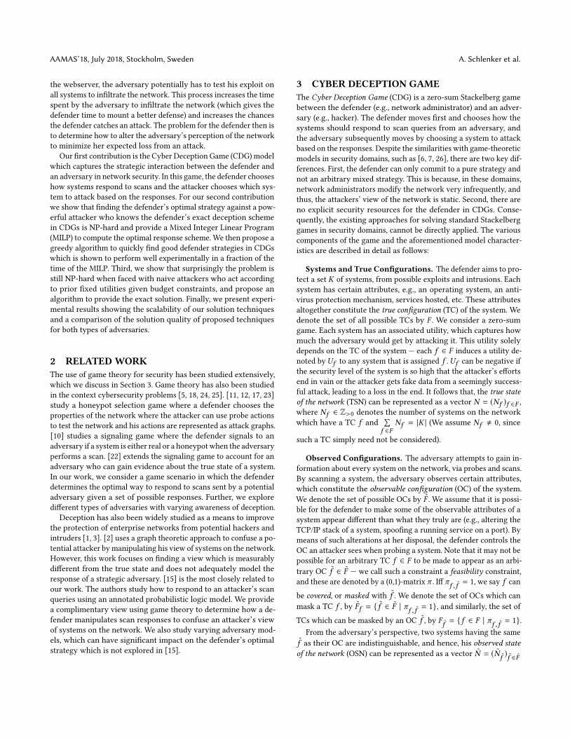
Figure 1: Simple example of an enterprise network.
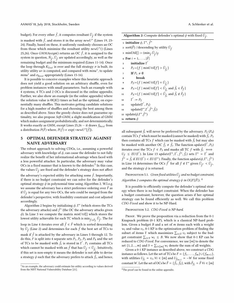
Figure 1 shows a simple example enterprise network which
will be used as a running example. We have a set of systems K ={k1,k2,k3}, set of TCs F = { f1, f2, f3} (shown in Figure 1 as the
green boxes) and set of OCs F = { ˜f1, ˜f2} (shown in Figure 1 as the
yellow boxes). Let the feasibility constraints be given by the sets
F˜f1= { f1, f2} and F
˜f2= { f2, f3}. The TCs are as follows:
f1 = [[os] L, [web] T, [ssh] O, [files] S]
f2 = [[os] L, [web] N, [ssh] O, [files] P]
f3 = [[os] W, [web] N, [ssh] O, [files] I]
For the TCs, the utilities are Uf1 = 10, Uf2 = 0, and Uf3 = 6. The
OCs are as follows:
˜f1 = [[os] L, [web] T]˜f2 = [[os] W, [web] T]
For simplicity, let all the costs c(f , ˜f ) to be 0, so that there is essen-
tially no budget constraint. Based on the TCs assigned as shown,
the state of the network (Nf )f ∈F is (1, 1, 1). When the defender
assigns OCs as shown in Figure 1, her strategy ϕ is given by
˜f1 ˜f2
f1 1 0
f2 1 0
f3 0 1
The expected utility of the adversary (loss of the defender) when
he attacks˜f1 or ˜f2 is respectively given by U
˜f1= (10+ 0)/2 = 5 and
U˜f2= 6/1 = 6. Thus, attacking
˜f2 leads to highest expected utility
for the attacker.
AAMAS’18, July 2018, Stockholm, Sweden A. Schlenker et al.
AdversaryKnowledge andUtility Estimation. The attacker’sawareness of the deception and the understanding of the defender’s
strategy may vary. Note that if the adversary is always able to find
the OC with highest expected utility, it is the worst case scenario
for the defender given the game is zero-sum. An attacker who is
fully aware of how the defender send the false responses to scan
requests (via insider threats, information leakage, etc.) would have
such ability. Formally, we define a powerful attacker to be one who
knows F , F , π , U and ϕ and chooses to attack the OC with the
(correct) highest expected utility U˜f computed through Equation
5. If the defender chooses a strategy that minimizes the expected
utility of a powerful attacker, she gets a robust strategy as the de-
fender can be assured that no matter the extent of the adversary’s
knowledge, no strategy he plays can lead to a greater loss for the
defender, in alignment with the minimax principle.
However, the attacker may not be so powerful. On the other
end of the spectrum, if the attacker is unaware of the defender’s
precise deception scheme or has a very limited understanding of
situation such that he cannot make any meaningful inference, his
decision making would be completely dependent on the observed
configurations of the systems and some fixed preferences over OCs
in terms of the estimated expected utility. Formally, we define a
naive attacker to be one who chooses to attack an existing OC˜f
(i.e., one at least one system is configured to have) with the highest
U˜f where U
˜f is not dependent on the defender’s strategy and is
known to the defender. This is also equivalent to the case where
the attacker just has a fixed preference of the OCs. We analyze
CDGs with powerful attackers in Section 4, and CDGs with naive
attackers in Section 5.
4 OPTIMAL DEFENDER STRATEGY AGAINSTPOWERFUL ADVERSARY
In this section, we compute the defender’s optimal strategy in a
CDG assuming a powerful adversary. The adversary attacks an
OC from the set argmax˜f ∈F U ˜f and gets an expected utility of
max˜f ∈F U ˜f , denoted in short as U ∗(ϕ), which is also the defender’s
expected loss. Hence, the defender aims to minimize it by choosing
her ϕ from the set argminϕ∈Φ U∗(ϕ).
4.1 Computational ComplexityWe call the problem of finding optimal defender strategy against a
powerful adversary in a CDG as CDG-Robust .We first investigate a special case. The following proposition
which provides a tight lower bound on minϕ∈Φ U∗(ϕ).
Proposition 4.1. The expected loss of the defender when playingher optimum strategy, is no lower than the average utility of thesystems, i.e.,
min
ϕU ∗(ϕ) ≥ UAve(K) =
∑f ∈F Nf Uf
|K |
Proof Sketch. Configuring the systems with different OCs effec-tively partitions the set K into subsets. Since the average utility ofall the systems in all these subsets is UAve(K), there exist at leastone subset whose average utility is no less than UAve(K). Therefore
the highest expected utility for the attacker, which is the maximumaverage utility of all these subsets, is no less thanUAve(K). 2
Thus, even when the defender plays her optimal strategy, the
attacker’s expected utility is at leastUAve(K). Consequently, if theinequality becomes tight for a strategy ϕ, it must be an optimal
strategy. It is easy to see that the bound becomes tight if and only
if U ∗(ϕ) = U˜f (ϕ), ∀ ˜f . Clearly, this is true if and only if U
˜f is the
same for each˜f set on any system, trivially so, if only a single OC
is set on all the systems. Thus,
Corollary 4.2. If it is feasible for the defender to set the sameOC on all the systems making them all indistinguishable to the ad-versary, doing so is an optimal strategy. Formally, if ∃ ˜f ∗ s.t. ∃ϕ∗ ∈Φ where ϕ∗
f , ˜f ∗= Nf ,∀f , then ϕ∗ ∈ argminϕ∈Φ U
∗(ϕ).
It is possible to efficiently check if such an OC exists, by enumer-
ation. However, it may not exist, and we show that CDG-Robust isNP-hard in general.
Proposition 4.3. CDG-Robust is NP-hard.
Proof. We prove the result via a reduction from the Partition
problem (PART ) which is known to be NP-complete. Given a multi-
set S of n positive integers that sum up to 2r , PART is the decision
problem to determine if S can be partitioned into two subsets S1
and S2 such that the sum of integers in S1, and S2 is r each. It canbe reduced to CDG-Robust as follows.
Let the input to PART be a set of integers S = {s1, . . . , sn } whoseelements sum to 2r . To construct a CDG, let the set of TCs be
F = { f1, . . . , fn } ∪ { fn+1, fn+2}, with utilities Ufi = si for eachi ∈ {1, . . . ,n} and Ufn+1
= Ufn+2= −r . Next, let there be n + 2
systems, each having a different TC. Let the set of OCs be F =
{ ˜f1, ˜f2}, with Ffi = F for each i ∈ {1, . . . ,n}, and Ffn+1= { ˜f1},
Ffn+2= { ˜f2}. Let all the costs be 0 so that the budget constraint
can be ignored. Assuming the adversary to be powerful, these
components completely define a CDG-Robust problem.
Note that, by Proposition 4.1 and the fact that
∑f Uf = 0, we
know that the optimal strategy ϕ must have U ∗(ϕ) ≥ 0. Now,
suppose S can be partitioned in subsets S1 and S2 such that the
numbers in each sum to r . Then, consider the strategy ϕ which
masks the TCs in { fi |si ∈ S1} and fn+1 with˜f1, and masks the TCs
in { fi |si ∈ S2} and fn+2 with˜f2. It is easy to check that U
˜f1(ϕ) =
U˜f2(ϕ) = 0 = U ∗(ϕ), making ϕ an optimal strategy. On the other
hand, suppose the defender’s optimal ϕ yields U ∗(ϕ) = 0. Since˜f1
must mask fn+1, and˜f2 must mask fn+2, neither of the OCs are
unused. Since U ∗(ϕ) = 0, w.l.o.g., assume U˜f1= 0. Hence, the sum
of utilities of the TCs masked with˜f1 must be 0. Therefore, the sum
of utilities of TCs masked by˜f ′ is also 0. Then, S1 = {si |ϕfi , ˜f1
=
1}, and S2 = {si |ϕfi , ˜f2= 1} form a partition of S , each having
sum of the elements r . It follows that, PART should output YESiff CDG-Robust finds an optimal strategy ϕ with U ∗(ϕ) = 0. This
reduction, being polynomial-time, proves the claim.
□
2A detailed proof can be found in the online appendix: https://www.dropbox.com/s/
n3wn0glm2clzs7e/Appendix.pdf?dl=0
Deceiving Cyber Adversaries: A Game Theoretic Approach AAMAS’18, July 2018, Stockholm, Sweden
4.2 The Defender’s Optimization ProblemThe defender’s optimal strategy ϕ can be computed by solving the
optimization problem given below.
min
u,ϕu (6a)
s.t. u∑f ∈F
ϕf , ˜f ≥∑f ∈F
ϕf , ˜f Uf ∀ ˜f ∈ ˜f (6b)
Constraints (1) ∼ (4)
The objective function in Equation (6a) minimizes the utility uthe adversary receives for the game. Equation (6b) enforces that
the adversary chooses a best response to the defender’s strategy ϕ,
where the expected utility for attacking a given˜f is given by (5).
Constraints (1)∼(4) represent a feasible defender strategy.This optimization problem is non-convex due to constraint (6b),
which can be linearized, to convert the optimization problem to
an MILP as follows. First, we devise an alternate representation of
defender’s strategy ϕ, as a |K | × |F | (0,1)-matrix σ , where σk, ˜f = 1
denotes system k is masked with˜f . Further, we represent the TSN
N via a vector x, where xk ∈ F represents the TC for system k .Then, for each TC f , we have Nf = |Kf | where, Kf = {k ∈ K |xk = F }, and ϕf , ˜f =
∑k ∈Kf σk, ˜f ∀f ,∀ ˜f . Hence, the alternate
representations are indeed equivalent. Then, constraints equivalent
to (1)∼(4) can be easily formulated for σ and x with an additional
constraint
∑˜f ∈F σk, ˜f = 1 ∀k ∈ K to ensure feasibility. More
importantly, equation (6b) can be reformulated as
u∑k ∈K
σk, ˜f ≥∑k ∈K
σk, ˜f Uxk ∀ ˜f ∈ F (7)
The left hand side of (7) can be seen as the sum of a set of terms
uσk, ˜f , each of which is the product of binary variable σk, ˜f and
the continuous variable u. Such an expression can be linearized by
introducing variables zk, ˜f for each k ∈ K and˜f ∈ F , and enforcing
zk, ˜f = uσk, ˜f . Consequently, we can rewrite (7) as:∑k ∈K
zk, ˜f ≥∑k ∈K
σk, ˜f Uxk (8)
To enforce zk, ˜f = uσk, ˜f , we consider u ∈ [Umin ,Umax ] where
Umin = minf ∈F Uf and Umax = maxf ∈F Uf . With these bounds
on u, we then include the constraints for each z variable in the
optimization problem as follows:
Uminσk, ˜f ≤ zk, ˜f ≤ Umaxσk, ˜f (9)
u − (1 − σk, ˜f )Umax ≤ zk, ˜f ≤ u − (1 − σk, ˜f )U
min(10)
After this conversion the optimization problem becomes an MILP.
The complete formulation can be found in the online appendix.
4.3 Greedy-Minimax AlgorithmDespite the speedup via cut generation, solving the above MILP
can still be computationally expensive for large instances. Hence,
we seek heuristic algorithms which may be suboptimal but run fast
and perform well on average. In this section, we describe a simple
approach to sequentially assign OCs to the systems, by greedily
minimizing attacker’s maximum expected utility for the partially
built strategy at each stage. Algorithm 1 gives the pseudo-code.
Algorithm 1: Greedy-Minimax
1 minIndCost[] ← (min˜f c(f , ˜f ))f ∈F
2 minTotCost ← ∑f Nf ∗minIndCost[f ]
3 initializeminu∗, σbest4 For iter = 1 . . .numIter
5 Kl ist [] ← shu f f le(K)6 initialize remB ← B, reqB ←minTotCost
7 initialize σ [], N [], U []8 For i = 1 . . . |K |9 k ← Kl ist [i], f ← x[k]
10 σ [k] ← GMMAssiдn(f ,σ [], N , U [])11 N [σ [k]] ← N [σ [k]] + 1
12 update(U [σ [k]])13 remB ← remB − c(f ,σ [k])14 reqB ← reqB −minIndCost[f ]15 compute u∗ = max
˜f U [ ˜f ])16 update(minu∗,u∗,σbest ,σ )17 return σbest18 Procedure GMMAssiдn(f ,σ [], N , U [])19 initialize newU ∗[]20 For ˜f ∈ Ff21 If (reqB −minIndCost[f ] + c(f , ˜f ) > remB) Then22 Continue23 σ [k] ← ˜f
24 newU ∗[ ˜f ] ← U ∗(σ )25 Fbest ← argmin
˜f newU∗[ ˜f ]
26 generate ˜fbest ∼ uniRand(Fbest )27 return ˜fbest
Greedy-Minimax starts by computing for each f ∈ F , the min-
imum cost of masking f with any feasible OC, and subsequently,
the minimum total cost of masking all the systems (Lines 1-2). Next,
σbest andminu∗ are initialized, which respectively denote the fi-
nal output strategy of the algorithm and the corresponding utility
(Line 3). Subsequently, the algorithm is conducted in a number of
iterations. In each iteration, a random shuffle of the set of systems
is obtained, referred to as Kl ist above. Subsequently, the strategyσ which is a candidate solution corresponding to this shuffle, the
corresponding observed state of the network (N˜f ) ˜f ∈F , and the cor-
responding utilities (U˜f ) ˜f ∈F are all initialized. These are constantly
maintained as the algorithm loops through Kl ist , building the so-lution by assigning an OC to a system one by one (Lines 8-10).
The OC to be assigned for a system is determined via the function
GMMAssiдn() which is the essence of this heuristic algorithm. The
input to this function is the TC f of the system in question, and
the currently built solution in terms of σ , N , U . Given these, the
function considers the candidate OCs in F one by one, refutes those
which lead to violation of the budget constraint (i.e., make the resul-
tant minimum required budget to exceed the resultant remaining
AAMAS’18, July 2018, Stockholm, Sweden A. Schlenker et al.
budget). For every other˜f , it computes resultant U
˜f if the system
is masked with˜f , and stores it in the array newU ∗ (Lines 19, 23-
24). Finally, based on these, it uniformly randomly chooses an OC
from those which minimize the resultant utility newU ∗() (Lines25,26). Once GMMAssiдn() returns an OC
˜f , it is assigned to the
system in question, N˜f , U ˜f are updated accordingly, as well as the
remaining budget and the minimum required (Lines 11-14). Once
the loop through Kl ist is over and the full strategy σ is built, its
utility utility u∗ is computed, and compared withminu∗, to update
minu∗ and σbest appropriately (Lines 15-16).
It is possible to conceive examples where this heuristic approach
does not yield a good solution on an arbitrary shuffle, even for
problem instances with small parameters. Such an example with
4 systems, 4 TCs and 2 OCs is discussed in the online appendix.
Further, we also show an example (in the online appendix) where
the solution value is Θ(|K |) times as bad as the optimal, on expo-
nentially many shuffles. This motivates getting candidate solutions
for a high number of shuffles and choosing the best among them
as described above. Since the greedy choice does not guarantee op-
timality, we also propose Soft-GMM, a slight modification of GMM
which makes assignment probabilistically, and not deterministically.
It works exactly as GMM, except Lines 25,26 — it draws fbest from
a distribution P(F ) where, P( ˜f ) ∝ exp(−newU ∗[ ˜f ]).
5 OPTIMAL DEFENDER STRATEGY AGAINSTNAIVE ADVERSARY
The robust approach to solving CDGs, i.e., assuming a powerful
adversary with knowledge of ϕ, can cause the defender to not fully
realize the benefit of her informational advantage when faced with
a less powerful attacker. In particular, the adversary may value
OCs in a fixed manner that is known to the defender.3In this case,
the values U˜f are fixed and the defender’s strategy does not affect
the adversary’s expected utility for attacking some˜f . Importantly,
if there is no budget constraint we can solve for the defender’s
optimal strategy ϕ in polynomial time using Algorithm 2. W.l.o.g.
we assume the adversary has a strict preference ordering over F as
if U˜f is equal for any two OCs, the sets could be merged from the
defender’s perspective, with feasibility constraint and cost adjusted
accordingly.
Algorithm 2 begins by initializing ϕ, Γ∗ (which stores the TCs
the adversary attacks) and˜f ∗ (the OC the adversary attacks given
ϕ). In Line 3 we compute the matrix minUtil[] which stores the
lowest utility achievable for each TC which is min˜f ∈Ff U ˜f . The for
loop in Line 4 iterates over all˜f ∈ F which is sorted descending
by U˜f (Line 2) and determines for each
˜f the best set of TCs to
mask if˜f is attacked by the adversary in Lines 5 through 12. To
do this, F is split into 4 separate sets P1, P2, P3 and P4 and the set
of TCs to be masked with˜fi is stored in Γ
′. P1 contains all TCs
which cannot be masked with an˜f that has U
˜f < U˜fi. Intuitively,
if this set is non-empty it means the defender is not able to devise
a strategy ϕ such that the adversary prefers to attack˜fi , and hence,
3As an example, the adversary could estimate his utility according to values derived
from the NIST National Vulnerability Database [21].
Algorithm 2: Compute defender’s optimal ϕ with fixed U˜f .
1 initialize ϕ, Γ∗, ˜f ∗
2 sort(F ) //descending by utility U˜f
3 minUtil[] := (min˜f U ˜f )f
4 For i = 1, . . . , |F |5 initialize Γ
′
6 P1:={ f |minUtil[f ] > U˜fi}
7 If P1 , ∅8 break9 P2:={ f |minUtil[f ] = U
˜fi}
10 P3:={ f |minUtil[f ] < U˜fiand
˜fi ∈ Ff }11 P4:={ f |minUtil[f ] < U
˜fiand
˜fi < Ff }12 Γ
′:= P2
13 update(Γ′, P3)
14 update(Γ∗,Γ′,
˜f ∗, ˜fi )
15 update(ϕ,Γ∗, ˜f ∗)16 return ϕ
all subsequent˜fi will never be preferred by the adversary. P2 (P4)
contain TCs f whichmust bemasked (cannot bemasked) with˜fi . P3
then contains all TCs f which can be masked with˜fi but may also
be masked with another OC˜fj , ˜fi . The function update(Γ′ , P3)
iterates over the TCs f ∈ P3 and masks all TC f with˜fi ⇐⇒
Uf ≤ EU (Γ′). In Line 13 update(Γ∗, Γ′ , ˜f ∗, ˜fi ) sets Γ∗ = Γ′and
˜f ∗ = ˜fi if EU (Γ′) < EU (Γ∗). Finally, the function update(ϕ, Γ∗, ˜f ∗)
in Line 14 determines the OCs˜f′for all f < Γ∗ given U
˜f ′ < U˜f ∗
and the strategy ϕ is returned.
Proposition 5.1. Given fixed utilities U˜f and no budget constraint,
Algorithm 2 computes the optimal strategy ϕ in O(|F | |F |). 4
It is possible to efficiently compute the defender’s optimal strat-
egy when there is no budget constraint. When the defender has
a budget constraint, however, the question arises if her optimal
strategy can be found efficiently as well. We call this problem
CDG-Fixed and show it to be NP-Hard.
Proposition 5.2. CDG-Fixed is NP-hard.
Proof. We prove the proposition via a reduction from the 0-1
Knapsack problem (0-1 KP), which is a classical NP-hard prob-
lem. Given a budget B and a set of m items each with a weight
wi and value vi , 0-1 KP is the optimization problem of finding the
subset of items Y which maximizes
∑i ∈Y vi subject to the bud-
get constraint
∑i ∈Y wi ≤ B. We now show that 0-1 KP can be
reduced to CDG-Fixed . For convenience, we use [m] to denote the
set {1, 2...,m} and S = ∑i ∈[m]wi denote the sum of all weights.
Given a 0-1 KP instance as described above, we construct a CDG
instance as follows. Let the set of TCs be F = { f1, . . . , fm }∪{ fm+1},with utilities Ufi = vi ,∀i ∈ [m] and Ufm+1
= −W for some fixed
constantW . Let the set of OCs be F = { ˜f1, ˜f2}, with Ffi = F ∀i ∈ [m]4The proof can be found in the online appendix.
Deceiving Cyber Adversaries: A Game Theoretic Approach AAMAS’18, July 2018, Stockholm, Sweden
and Ffm+1= { ˜f1}. Set the costs as c(fi , ˜f1) = 0, c(fi , ˜f2) = wi
for all i ∈ [m] and c(fm+1, ˜f1) = 0. Set U˜f1> U
˜f2. Assuming a
naive adversary, these components completely define aCDG-Fixed
problem. Since fm+1 is bound to be masked by˜f1, and U ˜f1
> U˜f2,
attacking˜f1 is a dominant strategy for the adversary.
Observe that
∑f ∈F Uf is
∑i ∈[m]wi −W = S −W . We claim
that the optimal objective of the 0-1 KP instance is greater than
S −W if and only if the optimal defender utility in the constructed
CDG-Fixed problem, i.e.,U ∗(ϕ), is negative. We first prove the⇐direction. Let ϕ∗ be the optimal solution to theCDG-Fixed problem.
By definition, the set Y = {i : ϕ∗fi , ˜f2= 1} is a feasible solution to
the 0-1 KP since the cost of mapping fi to ˜f2 iswi . The sum of total
weights is S −W whereas U ∗(ϕ∗) < 0 meaning the total weights
of configurations mapped to˜f1 is less than 0, this implies that the
total weights of configurations mapped to˜f2 is at least S −W . So
the optimal objective of the 0-1 KP is also at least S −W . The⇒direction follows a similar argument.
The above claim shows that for any constantW , we can check
whether the optimal objective of the 0-1 KP is greater than S −Wby solving anCDG-Fixed instance. Using this procedure as a black-
box, we can perform a binary search to find the exact optimal
objective of the 0-1 KP with integer values within O(poly(log(S)))steps (both S and weights are machine numbers with input size
O(log(S))). As a result, we have constructed a polynomial time
reduction from computing the optimal objective of any given 0-1 KP
to solving the CDG-Fixed problem. This implies the NP-hardness
of the CDG-Fixed problem. □
CDG-Fixed can be solved with Algorithm 2 via a modification
to the function update(Γ′ , P3) in Line 13. Given Γ′, we compute the
minimum budget B′required to mask all TCs f ∈ Γ
′with
˜fi and
mask all TCs f ∈ P3 and f ∈ P4 with˜fj such that U
˜fj< U
˜fi. If
Γ′= ∅, then for f ∈ P3 wemask f with ˜fi if c(f , ˜fi ) < B
′. Assuming
P3 is sorted ascending, once the defender assigns˜fi to a TC f she is
done. If Γ′, ∅, the defender must solve at n = nΓ′ , . . . , |K | (where
nΓ′ = |Γ′ |) MILPs, given in Problem (11a), to find the best Γ
′. Denote
uΓ′ = EU (Γ′).
min
ϕnΓ′uΓ′ +
∑f
ϕf , ˜f Uf (11a)
s.t.
∑f
ϕf , ˜fi≤ n − nΓ′ (11b)
Constraints (1) ∼ (4)
6 EXPERIMENTSWe evaluate the CDG model and solution techniques using synthet-
ically generated game instances. The game payoffs are set to be
zero-sum, and for each TC, the payoffsUf are uniformly distributed
in [1, 10]. Each OC˜f is randomly assigned a set of TCs it can mask,
while ensuring each TC can be masked with at least one OC. To
generate a network state x, each system is randomly assigned a TC
uniformly at random. The costs c(f , ˜f ) are uniformly distributed
in [1, 100] with the budget B uniformly distributed in-between the
minimum cost assignment and maximum cost assignment. All ex-
periments are averaged over 30 randomly generated game instances
and have 50 TCs.
6.1 Powerful Adversary - Scalability andSolution Quality Loss
0
20
40
60
80
100
10 12 14 16 18 20
Ru
nti
me
(s)
Num of Observables
MILP
GMM
(a) All-powerful Adversary
4
5
6
7
8
10 12 14 16 18 20
Ad
ve
rsa
ry U
tili
ty
Num of Observables
MILP
GMM
(b) Fixed Utilities
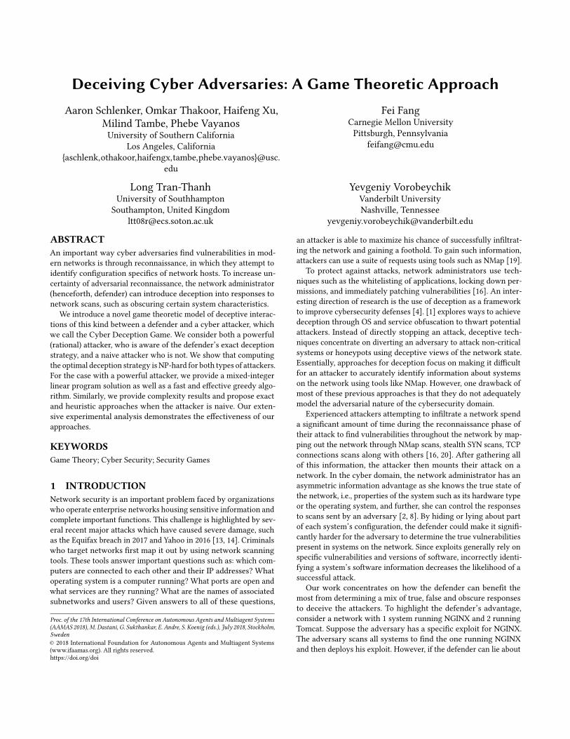
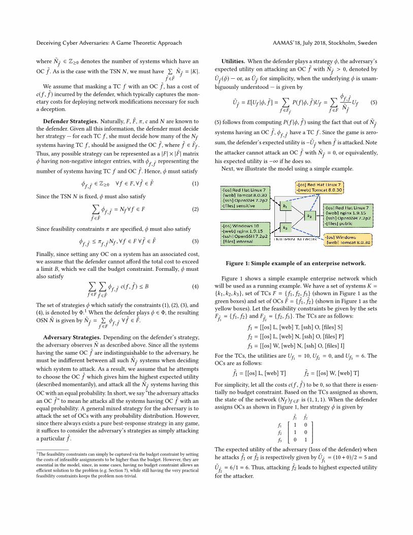
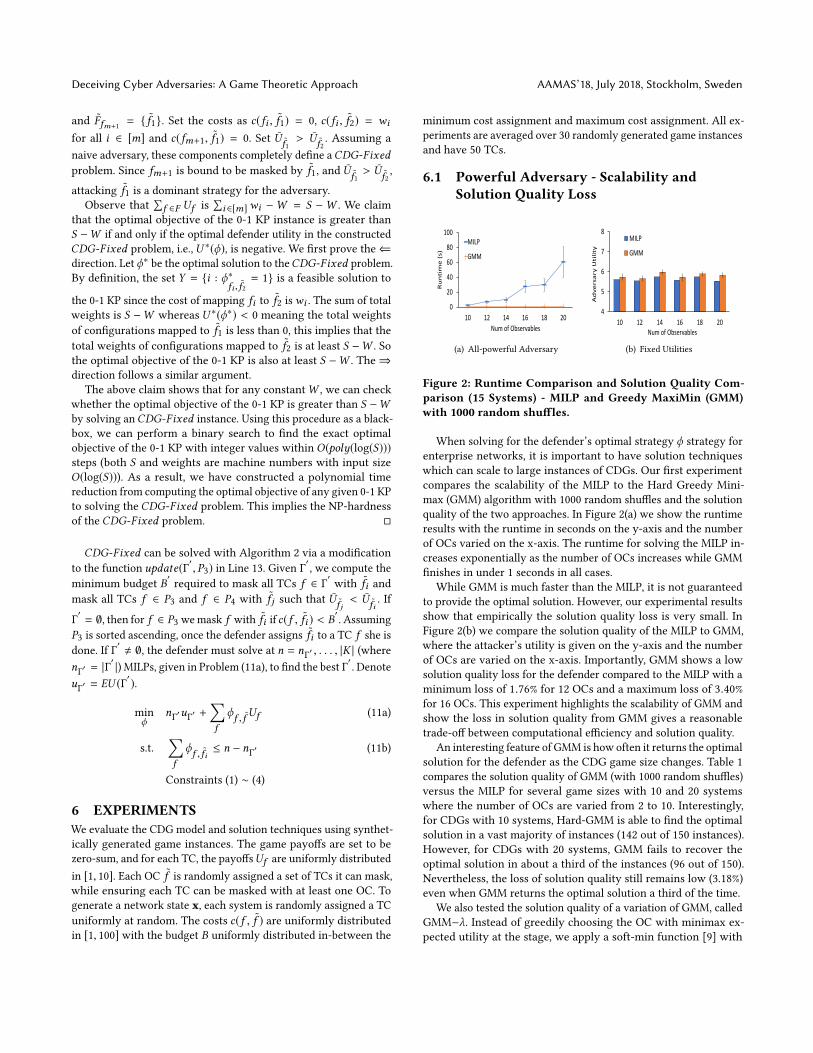
Figure 2: Runtime Comparison and Solution Quality Com-parison (15 Systems) - MILP and Greedy MaxiMin (GMM)with 1000 random shuffles.
When solving for the defender’s optimal strategy ϕ strategy for
enterprise networks, it is important to have solution techniques
which can scale to large instances of CDGs. Our first experiment
compares the scalability of the MILP to the Hard Greedy Mini-
max (GMM) algorithm with 1000 random shuffles and the solution
quality of the two approaches. In Figure 2(a) we show the runtime
results with the runtime in seconds on the y-axis and the number
of OCs varied on the x-axis. The runtime for solving the MILP in-
creases exponentially as the number of OCs increases while GMM
finishes in under 1 seconds in all cases.
While GMM is much faster than the MILP, it is not guaranteed
to provide the optimal solution. However, our experimental results
show that empirically the solution quality loss is very small. In
Figure 2(b) we compare the solution quality of the MILP to GMM,
where the attacker’s utility is given on the y-axis and the number
of OCs are varied on the x-axis. Importantly, GMM shows a low
solution quality loss for the defender compared to the MILP with a
minimum loss of 1.76% for 12 OCs and a maximum loss of 3.40%
for 16 OCs. This experiment highlights the scalability of GMM and
show the loss in solution quality from GMM gives a reasonable
trade-off between computational efficiency and solution quality.
An interesting feature of GMM is how often it returns the optimal
solution for the defender as the CDG game size changes. Table 1
compares the solution quality of GMM (with 1000 random shuffles)
versus the MILP for several game sizes with 10 and 20 systems
where the number of OCs are varied from 2 to 10. Interestingly,
for CDGs with 10 systems, Hard-GMM is able to find the optimal
solution in a vast majority of instances (142 out of 150 instances).
However, for CDGs with 20 systems, GMM fails to recover the
optimal solution in about a third of the instances (96 out of 150).
Nevertheless, the loss of solution quality still remains low (3.18%)
even when GMM returns the optimal solution a third of the time.
We also tested the solution quality of a variation of GMM, called
GMM−λ. Instead of greedily choosing the OC with minimax ex-
pected utility at the stage, we apply a soft-min function [9] with
AAMAS’18, July 2018, Stockholm, Sweden A. Schlenker et al.
5
6
7
8
9
100 500 1000 2000
Adve
rsar
y Ut
ility
Num of Shuffles
MILP GMM-Hard
GMM-20 GMM-1
GMM-.001
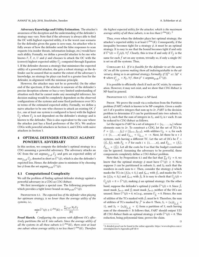
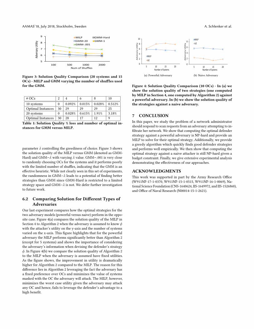
Figure 3: Solution Quality Comparison (20 systems and 15OCs) - MILP and GMM varying the number of shuffles usedfor the GMM.
# OCs 2 4 6 8 10
10 systems 0 0.092% 0.015% 0.028% 0.512%
Optimal Instances 30 29 29 29 25
20 systems 0 0.028% 0.615% 1.91% 3.18%
Optimal Instances 30 28 17 12 9
Table 1: Solution Quality % loss and number of optimal in-stances for GMM versus MILP.
parameter λ controlling the greediness of choice. Figure 3 shows
the solution quality of the MILP versus GMM (denoted as GMM-
Hard) and GMM−λ with varying λ value. GMM−.001 is very close
to randomly choosing OCs for the systems and it performs poorly
with the limited number of shuffles, indicating that the GMM is an
effective heuristic. While not clearly seen in this set of experiments,
the randomness in GMM−λ leads to a potential of finding better
strategies than GMM since GMM-Hard is restricted to a limited
strategy space and GMM−λ is not. We defer further investigation
to future work.
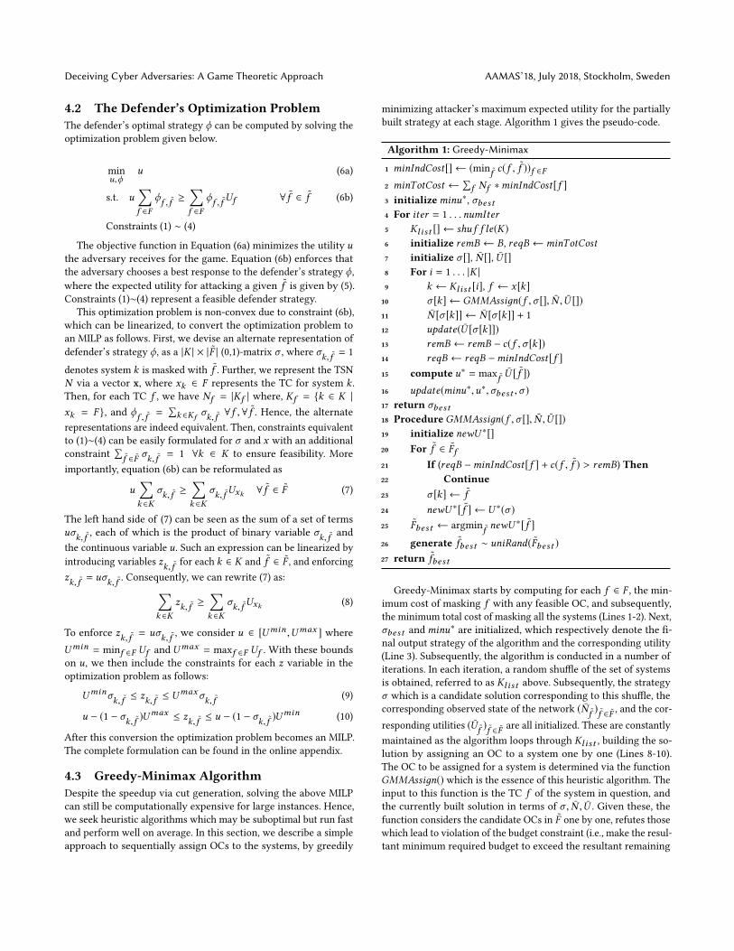
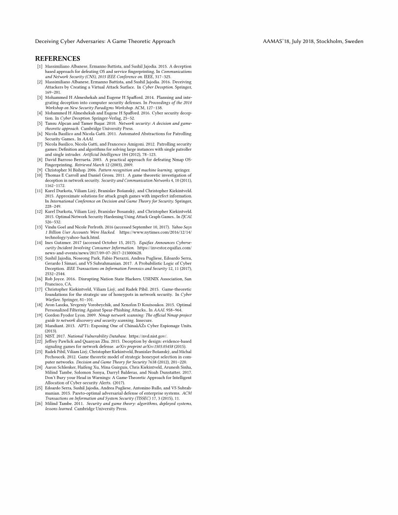
6.2 Comparing Solution for Different Types ofAdversaries
Our last experiment compares how the optimal strategies for the
two adversary models (powerful versus naive) perform in the oppo-
site case. Figure 4(a) compares the solution quality of the MILP in
Section 4 to Algorithm 2 when the adversary is assumed to know ϕwith the attacker’s utility on the y-axis and the number of systems
varied on the x-axis. This figure highlights that for the powerful
adversary the MILP performs significantly better than Algorithm 2
(except for 5 systems) and shows the importance of considering
the adversary’s information when devising the defender’s strategy
ϕ. In Figure 4(b) we compare the solution quality of Algorithm 2
to the MILP when the adversary is assumed have fixed utilities.
As the figure shows, the improvement in utility is dramatically
higher for Algorithm 2 compared to the MILP. The reason for this
difference lies in Algorithm 2 leveraging the fact the adversary has
a fixed preference over OCs and minimizes the value of systems
masked with the OC the adversary will attack. The MILP, however,
minimizes the worst case utility given the adversary may attack
any OC and hence, fails to leverage the defender’s advantage to a
high benefit.
0
2
4
6
8
10
5 10 15 20
Ad
ve
rsa
ry U
tili
ty
Number of Systems
MILP
UE
(a) Powerful Adversary
0
2
4
6
8
5 10 15 20
Ad
ve
rsa
ry U
tili
ty
Number of Systems
MILP
UE
(b) Naive Adversary
Figure 4: Solution Quality Comparison (10 OCs) - In (a) weshow the solution quality of two strategies (one computedbyMILP in Section 4, one computed by Algorithm 2) againsta powerful adversary. In (b) we show the solution quality ofthe strategies against a naive adversary.
7 CONCLUSIONIn this paper, we study the problem of a network administrator
should respond to scan requests from an adversary attempting to in-
filtrate her network. We show that computing the optimal defender
strategy against a powerful adversary is NP-hard and provide an
MILP to solve for their optimal strategy. Additionally, we provide
a greedy algorithm which quickly finds good defender strategies
and performs well empirically. We then show that computing the
optimal strategy against a naive attacker is still NP-hard given a
budget constraint. Finally, we give extensive experimental analysis
demonstrating the effectiveness of our approaches.
ACKNOWLEDGMENTSThis work was supported in part by the Army Research Office
(W911NF-17-1-0370, W911NF-15-1-0515, W911NF-16-1-0069), Na-
tional Science Foundation (CNS-1640624, IIS-1649972, and IIS-1526860),
and Office of Naval Research (N00014-15-1-2621).
Deceiving Cyber Adversaries: A Game Theoretic Approach AAMAS’18, July 2018, Stockholm, Sweden
REFERENCES[1] Massimiliano Albanese, Ermanno Battista, and Sushil Jajodia. 2015. A deception
based approach for defeating OS and service fingerprinting. In Communicationsand Network Security (CNS), 2015 IEEE Conference on. IEEE, 317–325.
[2] Massimiliano Albanese, Ermanno Battista, and Sushil Jajodia. 2016. Deceiving
Attackers by Creating a Virtual Attack Surface. In Cyber Deception. Springer,169–201.
[3] Mohammed H Almeshekah and Eugene H Spafford. 2014. Planning and inte-
grating deception into computer security defenses. In Proceedings of the 2014Workshop on New Security Paradigms Workshop. ACM, 127–138.
[4] Mohammed H Almeshekah and Eugene H Spafford. 2016. Cyber security decep-
tion. In Cyber Deception. Springer-Verlag, 25–52.[5] Tansu Alpcan and Tamer Başar. 2010. Network security: A decision and game-
theoretic approach. Cambridge University Press.
[6] Nicola Basilico and Nicola Gatti. 2011. Automated Abstractions for Patrolling
Security Games.. In AAAI.[7] Nicola Basilico, Nicola Gatti, and Francesco Amigoni. 2012. Patrolling security
games: Definition and algorithms for solving large instances with single patroller
and single intruder. Artificial Intelligence 184 (2012), 78–123.[8] David Barroso Berrueta. 2003. A practical approach for defeating Nmap OS-
Fingerprinting. Retrieved March 12 (2003), 2009.
[9] Christopher M Bishop. 2006. Pattern recognition and machine learning. springer.[10] Thomas E Carroll and Daniel Grosu. 2011. A game theoretic investigation of
deception in network security. Security and Communication Networks 4, 10 (2011),1162–1172.
[11] Karel Durkota, Viliam Lisy, Branislav Bošansky, and Christopher Kiekintveld.
2015. Approximate solutions for attack graph games with imperfect information.
In International Conference on Decision and Game Theory for Security. Springer,228–249.
[12] Karel Durkota, Viliam Lisy, Branislav Bosansky, and Christopher Kiekintveld.
2015. Optimal Network Security Hardening Using Attack Graph Games.. In IJCAI.526–532.
[13] Vindu Goel and Nicole Perlroth. 2016 (accessed September 10, 2017). Yahoo Says1 Billion User Accounts Were Hacked. https://www.nytimes.com/2016/12/14/
technology/yahoo-hack.html.
[14] Ines Gutzmer. 2017 (accessed October 15, 2017). Equifax Announces Cyberse-curity Incident Involving Consumer Information. https://investor.equifax.com/
news-and-events/news/2017/09-07-2017-213000628.
[15] Sushil Jajodia, Noseong Park, Fabio Pierazzi, Andrea Pugliese, Edoardo Serra,
Gerardo I Simari, and VS Subrahmanian. 2017. A Probabilistic Logic of Cyber
Deception. IEEE Transactions on Information Forensics and Security 12, 11 (2017),
2532–2544.
[16] Rob Joyce. 2016. Disrupting Nation State Hackers. USENIX Association, San
Francisco, CA.
[17] Christopher Kiekintveld, Viliam Lisy, and Radek Píbil. 2015. Game-theoretic
foundations for the strategic use of honeypots in network security. In CyberWarfare. Springer, 81–101.
[18] Aron Laszka, Yevgeniy Vorobeychik, and Xenofon D Koutsoukos. 2015. Optimal
Personalized Filtering Against Spear-Phishing Attacks.. In AAAI. 958–964.[19] Gordon Fyodor Lyon. 2009. Nmap network scanning: The official Nmap project
guide to network discovery and security scanning. Insecure.[20] Mandiant. 2013. APT1: Exposing One of ChinaâĂŹs Cyber Espionage Units.
(2013).
[21] NIST. 2017. National Vulnerability Database. https://nvd.nist.gov/.[22] Jeffrey Pawlick and Quanyan Zhu. 2015. Deception by design: evidence-based
signaling games for network defense. arXiv preprint arXiv:1503.05458 (2015).[23] Radek Pıbil, Viliam Lisy, Christopher Kiekintveld, Branislav Bošansky, andMichal
Pechoucek. 2012. Game theoretic model of strategic honeypot selection in com-
puter networks. Decision and Game Theory for Security 7638 (2012), 201–220.
[24] Aaron Schlenker, Haifeng Xu, Mina Guirguis, Chris Kiekintveld, Arunesh Sinha,
Milind Tambe, Solomon Sonya, Darryl Balderas, and Noah Dunstatter. 2017.
Don‘t Bury your Head in Warnings: A Game-Theoretic Approach for Intelligent
Allocation of Cyber-security Alerts. (2017).
[25] Edoardo Serra, Sushil Jajodia, Andrea Pugliese, Antonino Rullo, and VS Subrah-
manian. 2015. Pareto-optimal adversarial defense of enterprise systems. ACMTransactions on Information and System Security (TISSEC) 17, 3 (2015), 11.
[26] Milind Tambe. 2011. Security and game theory: algorithms, deployed systems,lessons learned. Cambridge University Press.
AAMAS’18, July 2018, Stockholm, Sweden A. Schlenker et al.
8 APPENDIX8.1 Missing Proofs
Proof of Proposition 4.1.
Proof. Equivalently, we show that, U ∗(ϕ) ≥∑f ∈F Nf Uf|K | for all
ϕ. Fix any ϕ ∈ Φ. We have,
U ∗(ϕ) ≥ U˜f (ϕ) ∀ ˜f (by definition of U ∗(ϕ))
∴∑˜f ∈F
N˜f U∗(ϕ) ≥
∑˜f ∈F
N˜f U ˜f
∴ |K | · U ∗(ϕ) ≥∑˜f ∈F
∑f ∈F
ϕf , ˜f Uf (using (5))
=∑f ∈F
©«Uf∑˜f ∈F
ϕf , ˜f
ª®®¬ (re-ordering terms)
=∑f ∈F
Uf Nf (by definition of ϕ, Nf )
∴ U ∗(ϕ) ≥∑f ∈F Nf Uf
|K |Since the choice of ϕ was arbitrary, the claim follows. □
Proof of Proposition 6.1.
Proof. We first show that for each˜f ∈ F , Lines 5 through 13 in
Algorithm 2 computes the set Γ′with the minimum average value.
To see this, note that all TCs f ∈ P2 must be in Γ′while all TCs
f ∈ P4 cannot be included. In update(Γ′ , P3) (note P3 is given in
sorted order) the defender decides for each f ∈ P3 to include the
Nf TCs in Γ′ ⇐⇒ Uf ≤ EU (Γ′). At the end of this update, tt
follows that Γ′must be the minimum average set for
˜fi . Given that
the for loop in Line 4 iterates through all˜f ∈ F , it must be the case
that the optimal Γ∗ is returned for some˜f .
In Line 2, sorting F takes O(|F | log |F |) time and calculating
minUtil[] takes O(|F | |F |) time. For each iteration of the for loop
in Line 4, it takes O(|F |) time to split F into the sets the four sets
P1, P2, P3 and P4. It takes the function update(Γ′ , P3) at most |F |operations to update Γ
′while update(Γ∗, Γ′ , ˜f ∗, ˜fi ) takesO(1) time.
Hence, each iteration it takesO(|F |) time and hence,O(|F | |F |) time
for the for loop. Lastly, update(ϕ, Γ∗, ˜f ∗) takes at O(|F | |F |) time to
return the defender’s strategy ϕ as it must find an OC˜fj for each
f < Γ∗ with U˜fj< U
˜fi. □
8.2 Full Formulation of MILP for 6a
min
u,σ ,zu (12a)
s.t.
∑k ∈K
zk, ˜f ≥∑k ∈K
σk, ˜f Uxk ∀ ˜f ∈ ˜f (12b)∑˜f ∈F
σk, ˜f = 1 ∀k ∈ K (12c)
σk, ˜f ≤ πxk , ˜f ∀k ∈ F ,∀ ˜f ∈ F (12d)
∑˜f ∈F
∑k ∈K
σk, ˜f c(xk , ˜f ) ≤ B (12e)
Uminσk, ˜f ≤ zk, ˜f ≤ Umaxσk, ˜f ∀k ∈ F ,∀ ˜f ∈ F (12f)
u − (1 − σk, ˜f )Umax ≤ zk, ˜f ∀k ∈ F ,∀ ˜f ∈ F (12g)
zk, ˜f ≤ u − (1 − σk, ˜f )Umin ∀k ∈ F ,∀ ˜f ∈ F (12h)
σk, ˜f ∈ {0, 1} ∀k ∈ F ,∀ ˜f ∈ F (12i)
8.3 GMM ExamplesNote that the adversary’s utility U ∗(ϕ) for any strategy ϕ can be
at most |K | times the optimal valueminϕU∗(ϕ). This follows from
observing that for any strategy ϕ, we have U˜f ≤ max
f |Nf >0
Uf ∀ ˜f by
definition, and thus,U ∗(ϕ) ≤ max
f |Nf >0
Uf , whereasminϕU∗(ϕ) is at
least the average of all the system utilities by Proposition 4.1. Since
any choice a greedy heuristic makes can be potentially suboptimal,
one may intuitively expect its performance to be worse for a higher
number of choices to be made, that is, for larger sized inputs, and
relatively better for smaller inputs. However, we show an example
instance of a CDG where despite the input size (|F |, |K |, |F |) beingvery small, the (hard-)GMM algorithm in a particular iteration (i.e.,
when conducted on a particular shuffle of the systems) gives a
highly suboptimal solution.
Consider the set of systems K = {k1,k2,k3,k4}, the set of TCsF = { f1, f2, f3, f4} and the set of OCs F = { ˜f1, ˜f2}. Let the fea-
sibility constraints be given via the sets F˜f1= { f1, f2, f3} and
F˜f2= { f2, f3, f4}. Let each system ki have the TC fi , so that the
TSN (Nf )f ∈F is (1, 1, 1, 1). For the TCs, let the utilities beUf1 = 1,
Uf2 = 2, Uf3 = 30, and Uf4 = 40. For simplicity, let all the costs
c(f , ˜f ) to be 0, so that there is essentially no budget constraint.
Consider the ordering of the systems on which GMM is per-
formed to be: {k1,k2,k3,k4}. Then, the strategy σ computed by the
GMM on this ordering is as follows:
˜f1 ˜f2k1 1 0
k2 1 0
k3 1 0
k4 0 1
Accordingly, we have the expected utilities of OCs U
˜f1= (1 +
2 + 30)/3 = 11 and U˜f2= 40/1 = 40, and thus, adversary’s utility
is 40 for this strategy. The optimal solution, however, masks k1, k3
with˜f1 and k2, k4 with
˜f2 giving the expected utilities of the OCs:
U˜f1= (40+ 2)/2 = 21 and U
˜f2= (30+ 1)/2 = 15.5, thus, the optimal
being just 21.
Further, the following is an example of a CDG which shows the
GMM algorithm can perform Θ(|K |) as bad as the optimal solution
on exponentially many shuffles.
Consider the CDG instancewith the set of systemsK = {k1, . . . ,km },so that |K | =m. Let the set of TCs F = { f1, f2, f3} and the set of OCsF = { ˜f1, ˜f2}. Let the true state of the network be: x = (1, 2, 3, . . .)Let the feasibility constraints be given by the sets F
˜f1= { f1, f3}
and F˜f2= { f2, f3}. For the TCs, the utilities areUf1 = 1,Uf2 = 2000,
Deceiving Cyber Adversaries: A Game Theoretic Approach AAMAS’18, July 2018, Stockholm, Sweden
andUf3 = ϵ . For simplicity, let all the costs c(f , ˜f ) to be 0, so that
there is essentially no budget constraint.
The optimal solution to this CDG is to assign systems k2, . . . ,kmto be masked by
˜f2 with k1 being masked with˜f1. This gives the
following expected utilities: U˜f1= 1/1 = 1 and U
˜f2=
2000+(m−2)ϵm−1
=
2000
m−1+(m−2)ϵm−1
. Consider any shuffle which orders the systems
such that k1 is first and k2 is last (of which there are (m − 2)!).Given any ordering of this type, GMM assigns assigns systems
k3, . . . ,km to be masked with˜f1 and would assign k2 to be masked
with˜f2. The expected utilities given this assignment is the following:
U˜f1=
1+(m−2)ϵm−1
= 1
m−1+(m−2)ϵm−1
and U˜f2= 2000/1 = 2000. The
loss in this case is ≈ 2000
2000
m−1
= 1
m−1which is a Θ(|K |) loss.