NBER WORKING PAPER SERIES

DEBT INTO GROWTH:HOW SOVEREIGN DEBT ACCELERATED THE FIRST INDUSTRIAL REVOLUTION

Jaume VenturaHans-Joachim Voth

Working Paper 21280http://www.nber.org/papers/w21280

NATIONAL BUREAU OF ECONOMIC RESEARCH1050 Massachusetts Avenue

Cambridge, MA 02138June 2015

Ventura acknowledges support from the Spanish Ministry of Science and Innovation (ECO2011-23197),the Generalitat de Catalunya (2014SGR-830 AGAUR), the Barcelona GSE Research Network, andthe ERC (Advanced Grant FP7-249588-ABEP). Voth acknowledges support from the ERC (AdvancedGrant FP7-230515), the University of Zurich, and the SNF (100018-156197). The views expressedherein are those of the authors and do not necessarily reflect the views of the National Bureau of EconomicResearch.

NBER working papers are circulated for discussion and comment purposes. They have not been peer-reviewed or been subject to the review by the NBER Board of Directors that accompanies officialNBER publications.

© 2015 by Jaume Ventura and Hans-Joachim Voth. All rights reserved. Short sections of text, notto exceed two paragraphs, may be quoted without explicit permission provided that full credit, including© notice, is given to the source.

Debt into Growth: How Sovereign Debt Accelerated the First Industrial RevolutionJaume Ventura and Hans-Joachim VothNBER Working Paper No. 21280June 2015JEL No. E22,E25,E62,H56,H60,N13,N23

ABSTRACT

Why did the country that borrowed the most industrialize first? Earlier research has viewed the explosionof debt in 18th century Britain as either detrimental, or as neutral for economic growth. In this paper,we argue instead that Britain’s borrowing boom was beneficial. The massive issuance of liquidly tradedbonds allowed the nobility to switch out of low-return investments such as agricultural improvements.This switch lowered factor demand by old sectors and increased profits in new, rising ones such astextiles and iron. Because external financing contributed little to the Industrial Revolution, this boostin profits in new industries accelerated structural change, making Britain more industrial more quickly.The absence of an effective transfer of financial resources from old to new sectors also helps to explainwhy the Industrial Revolution led to massive social change – because the rich nobility did not lendto or invest in the revolutionizing industries, it failed to capture the high returns to capital in thesesectors, leading to relative economic decline.

Jaume VenturaCREIUniversitat Pompeu FabraRamon Trias Fargas, 25-2708005-BarcelonaSPAINand Barcelona GSEand also NBERjventura@crei.cat

Hans-Joachim VothUniversity of ZurichDepartment of EconomicsSchönberggasse 1CH-8001 Zurichand CREIvoth@econ.uzh.ch

DEBT INTO GROWTH 2

1. Introduction

Over the course of a century, a country accumulates towering debts, mainly tofinance foreign wars – it is fighting abroad in two years out of three. Could such acountry transition from centuries of stagnation to sustained growth? Surprisingly,the answer is yes – the Industrial Revolution in Britain occurred under such circum-stances. The Glorious Revolution of 1688 turned Britain into a credible borrower;subsequently, borrowing increased massively (North and Weingast 1989). From1692 to 1815, Britain’s debt rose from 5% to over 200% of GDP (Sussman andYafeh 2006; Barro 1987). The funds raised were not used to finance productivity-enhancing infrastructures, but instead to pay for overseas wars. During this period,Britain was at war for 76 years – 62% of the time. And yet, frequent wars and highdebt accumulation coincided with a remarkable transformation of the economy. Bythe end of the period, Britain’s productive capacity had grown by a factor of eight,allowing it to sustain a population that was four times larger and twice as rich.Having moved millions of people from the countryside to urban centers, it hadbecome the “workshop of the world”.

How could Britain industrialize while accumulating towering debts that financedmainly foreign wars? Earlier research concluded that debt accumulation in 18thcentury Britain was detrimental to industrialization since it reduced the savingsavailable for private investment: “Government borrowing had another ... effect.Capital was deflected from private to public uses, and some of the developmentsof the industrial revolution were once more brought to a halt” (T.S. Ashton 1948).Williamson (1984) used a calibrated model of the British economy to show thatthis crowding-out effect might have slowed output growth by as much as half ofthe potential growth rate. But crowding-out should work through interest rates,and there is little evidence that they increased.1 Barro (1987) argued that debtaccumulation had a neutral effect on industrialization since it raised total savingsinstead of reducing private investment.2 Note that both Williamson and Barroassume that the British economy possessed well-functioning credit markets.3 Thekey question is then how much private savings increased in anticipation of futuretaxes required to service the debt. Williamson’s answer is ‘not much’ while Barro’sview is ‘one-to-one’.

In this paper, we argue instead that Britain’s debt accumulation acceleratedindustrialization. We model the Industrial Revolution as the arrival of new, high-productivity technologies.4 Entrepreneurs invest in these new industries because

1Research on interest rates and the yield on private assets has found few effects of sovereignborrowing. See Mirowski (1981); Clark (2001); Quinn (2001); Sussman and Yafeh (2004). OnlyHeim and Mirowski (1987) found evidence that nominal interest rates were somewhat higherduring the Revolutionary Wars with France, but even then they found that real yields were lower.2Indeed, historians have noted the highly elastic supply of savings in 18th century Britain (Neal1995).3By this, we mean that they assume that no-arbitrage conditions generally held, and that interestrates on government bonds, for example, are informative of the tightness of private credit.4This is in the spirit of Hansen and Prescott (2001).

DEBT INTO GROWTH 3

profit rates are high. Initially, entrepreneurs are relatively poor and own a smallfraction of the economy’s savings. The lion’s share of capital is in the hands ofthe nobility. Earls and dukes invest in agriculture and traditional industries whereprofit rates are relatively low. Ideally, entrepreneurs would borrow massively fromnobles; this would lead to faster growth and a more rapid structural transformation.Financial frictions make his impossible: the banking sector is small and relativelyinefficient, and the stock market is hamstrung by government restrictions. Prejudicealso plays a role, as the nobility shied away from money-making activities. As aresult, entrepreneurs are forced to finance their investments out of reinvested profits;capital formation and industrialization are relatively slow.

In such a setting, sovereign debt accelerates structural change. Sovereign bondsare attractive to the nobility because they offer higher returns than investments inagriculture and traditional industries. Entrepreneurs, on the other hand, are nottempted to buy sovereign bonds because returns in the new industries are evenhigher. Therefore, sovereign debt reduces investments in agriculture and tradi-tional industries. Reduced labor demand in traditional sectors in turn depresseswages economy-wide, raising profit rates for entrepreneurs. Since reinvested prof-its provide most of their financing, this raises investment in new industries. Incombination, this will ensure that sovereign debt accelerates structural change andgrowth. In contrast to Williamson and Barro, we emphasize the role of frictions inprivate credit markets – before the 19th century, little external financing found itsway into new industries, despite huge profit opportunities. As we describe in sec-tion II, throughout the Industrial Revolution private credit was limited, expensive,and it provided almost no resources to the most dynamic sectors of the economy.

Our model highlights two features whose importance has become more apparentin recent years – the key role of resource reallocation and of credit market frictionsin development (Hsieh and Klenow 2009, Banerjee and Moll 2010 and Gancia andZilibotti 2009). The effects of credit market frictions is surveyed in Banerjee andDuflo (2005) and highlighted in recent research by, inter alia, Banerjee and Duflo(2014) and Banerjee and Munshi (2005) . Our emphasis on credit market frictionsin a context of uneven growth in different sectors is related to Song, Storesletten,and Zilibotti’s (2011) recent work on China. By emphasizing resource reallocationand credit market frictions, our model offers a unified explanation for key macroe-conomic aspects of the Industrial Revolution.

The first aspect is relatively slow growth at the start of the Industrial Revolution.One of the key insights from the last 30 years of research on the British economyafter 1700 is that growth was relatively slow before 1850, with output per capitarising at a rate of 1% p.a. or less (Crafts and Harley 1992; Antras and Voth 2003).As in the seminal work by Crafts (1985), structural change is the key characteristicof the industrialization process in our approach – the shift out of agriculture andinto industry. Our model offers one interpretation of why growth was not faster:

DEBT INTO GROWTH 4

slow capital formation slowed down structural change because it was limited by theself-financing ability of entrepreneurs.

A second aspect of the Industrial Revolution that our framework sheds light on isthe social change engendered by the Industrial Revolution. Britain’s nobility in 1700held the vast majority of wealth and political power; by 1900, its relative positionhad declined markedly. The nobility did not invest directly in new technologies; italso did not lend to capitalists, either directly or through the financial system. Hadthe nobility been able to finance the new class of entrepreneurs in a competitivewell-functioning credit market, it would have appropriated virtually all of the profitopportunities arising from the new technologies – and the Industrial Revolutionwould have generated little or no social change.5

A third aspect of the Industrial Revolution is limited gains in terms of livingstandards accruing to the working class. Real wages did not keep up with outputgrowth during the core phase of the industrialization process (1770-1830); the wageshare of national income fell sharply, while the share going to capital surged (Allen2009). Our model offers an explanation for this puzzling feature, by showing howmassive sovereign borrowing contributed to the divergence between productivityand wages. It is precisely the reduction of labor demand (because nobles switchedfrom low-return investments to sovereign debt) that kept wages low and generatedthe entrepreneurial profits needed to finance industrialization.

We deliberately abstract from other aspects of the Industrial Revolution. First,we take technological change as given. While the aggregate productivity statisticsdo not show it, the eighteenth century saw many important inventions and inno-vations, from the use of steam power to advances in cotton spinning, weaving, andtransport (Mokyr 1990). Nor do we seek to explain why these advances were firstconceived or implemented in Britain (Allen 2009). Furthermore, we do not examinethe role of new sources of energy (Wrigley 1990, Stokey 2001), nor of foreign trade(Crafts 1985, Crafts and Harley 2000, Temin 1997) or of improvements in transport(O´Rourke and Williamson 2005, Bogart 2009). Finally, we do not consider theimpact of institutional improvements (North and Weingast 1989, Mokyr and Nye2007). All these factors undoubtedly contributed to the Industrial Revolution inways small or large. Here, we focus on the factors that determined how quicklytechnological change made itself felt in the economy at large.

The rest of the paper is organized as follows. Section II provides the historicalbackground and context. It reviews the stylized facts of the Industrial Revolutionand it also describes the main features of the British financial system. Section IIIpresents our model and derives our analytical results. It also provides a very roughattempt at quantification. Section IV concludes.

5This depends on the relative bargaining powers of savers and investors in new technology. How-ever, since the nobility was small, it is likely that it would have exerted substantial market power.

DEBT INTO GROWTH 5

2. Historical Background

In this section, we first briefly summarize key macroeconomic features of theBritish Industrial Revolution, as well as of the political context. In addition, wediscuss the social and distributional consequences of the transition to self-sustaininggrowth, and we highlight the main features of the UK financial system.

2.1. War and the growth of debt in eighteenth-century England. The so-called Glorious Revolution in 1688 deposed James II from the throne. Parliamentinvited William of Orange to become monarch. The new constitutional settlementincluded major restrictions of the monarch’s powers, and a much-expanded role forParliament. Taxation required the parliamentary assent; the judicial powers of theking were severely curtailed (North and Weingast 1989).

At the time of the Glorious Revolution, Britain had only a small national debt.In the next 150 years, the total debt stock rose rapidly. Between 1692 and 1815,debt rose from 5% of GDP to more than 200% (Barro 1987). The cost of numerouswars that followed the accession of the Hanoverian kings to the throne was largelyresponsible. Britain found itself at war for 81 years, or almost 2 out of every 3. Theexpenditure on the armed forces was considerable, and constituted by far the singlemost important item of the government budget. A single ship of the line of theRoyal Navy cost more than all the capital in the most expensive iron-works builtat the time (Brewer 1990). In the period 1692-1815, spending on the Army, Navyand on ordinance was equivalent to 72% of total revenue. Once the debt servicecosts were added to this figure – due to the debts accumulated in wartime – therewas hardly any money left for non-military spending.

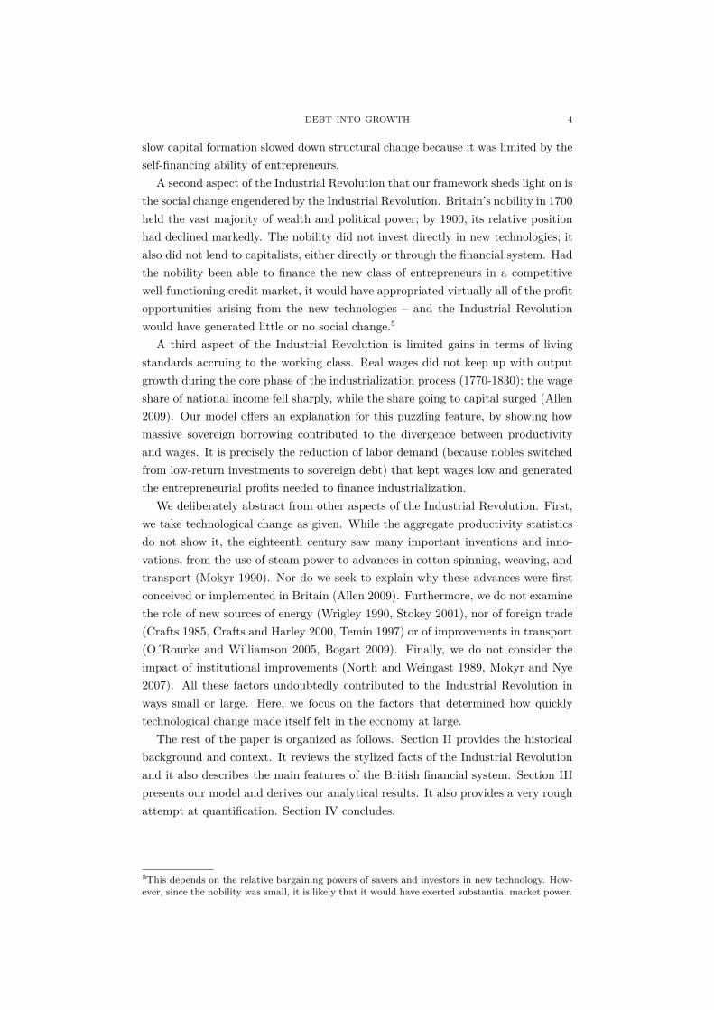
Figure 2.1 shows the path of overall expenditure and of total debt. Shaded areasindicate wars. Dramatic spikes in total spending almost always coincided withmajor wars. Almost the entire rise in debt during the eighteenth century occurredwhile Britain was fighting abroad. Once peace was concluded, debt levels typicallystabilized in nominal terms, and GDP growth reduced the debt burden over time.Peaking at over 200% after the end of the Napoleonic Wars, debt eventually fell to100% of GDP by the middle of the nineteenth century.

Due to frequent wars, borrowing needs were substantial. In addition, new finan-cial instruments facilitated the growth in public debt. Prior to the eighteenth cen-tury, most borrowing by the English Crown was complex and created liquid assets.So-called tallies – notched wooden sticks denoting various amounts of taxes payableto the government – were used to borrow. In effect, tally rods acted like short-datedIOUs issued by the government, backed by a specific tax stream. While these couldbe resold, trading was typically highly illiquid, with discounts of more than half offace value. After numerous experiments, the British government granted privilegesto several companies, in exchange for financing the public debt. The most impor-tant included the Bank of England, the New East India Company, and the SouthSea Company. All of these received royal charters in exchange for taking on some

DEBT INTO GROWTH 6

Figure 2.1. Debt and Expenditure in the UK, 1692-1860

of the government’s debts. In addition, government bonds were combined with anational lottery (Million Adventure). Life annuities were issued, as well as tontines.Short-term borrowing in case of war by the armed forces produced so-called armyand navy bills, effectively short-dated promises to pay. The biggest experiment ofall involved the South Sea Company, which offered to exchange all public debt in1720 for shares. A similar exercise in 1719 had been attractive to both the gov-ernment and the public, by improving the liquidity of outstanding debt. While theSouth Sea scheme ultimately failed, it demonstrated the attractions of liquid paperassets. The UK finally introduced consolidated annuities (“consols”), perpetualbonds with a relatively low interest rate (Dickson 1967). These were first issued in1751. Originally carrying a yield of 3.5%, they were eventually converted to 3% in1757 (and to 2.75% in 1888). Consols were liquidly traded, and became a primesavings vehicle for the moneyed classes in the UK.

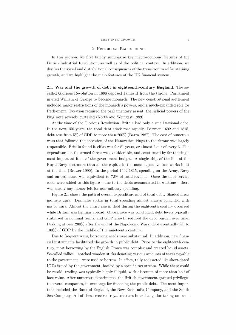
2.2. Britain’s growth and industrial transformation. Growth during theclassic period of the British Industrial Revolution (1760-1850) was slow by modernstandards. Initially, output growth per capita was barely faster than during thepre-industrial period.6 After the middle of the 18th century, growth acceleratedfrom around 1 % p.a. to 2.5%. At the same time, population increased rapidly,from 5.2 million to 19 million. Growth rates across sectors were highly unequal.Figure 2.2 shows annual GDP by sector. Agriculture expanded relatively slowlyover the period 1700-1860, increasing total output by a factor of 2.8 – a slower rateof increase than that of population.7 Over the same period, real GDP in servicesincreased 9-fold, and in industry, 14-fold (Broadberry et al. 2010) .

6Galor (2005) gives a figure of 0.1% p.a. for the pre-industrial era, while the work of Crafts andHarley suggests rates of 0.2% p.a. in the years 1760-1800.7For the effects of population pressure on economic structure, cf. Crafts and Harley (1992).

DEBT INTO GROWTH 7

Figure 2.2. Growth of Output in Britain, 1700-1860

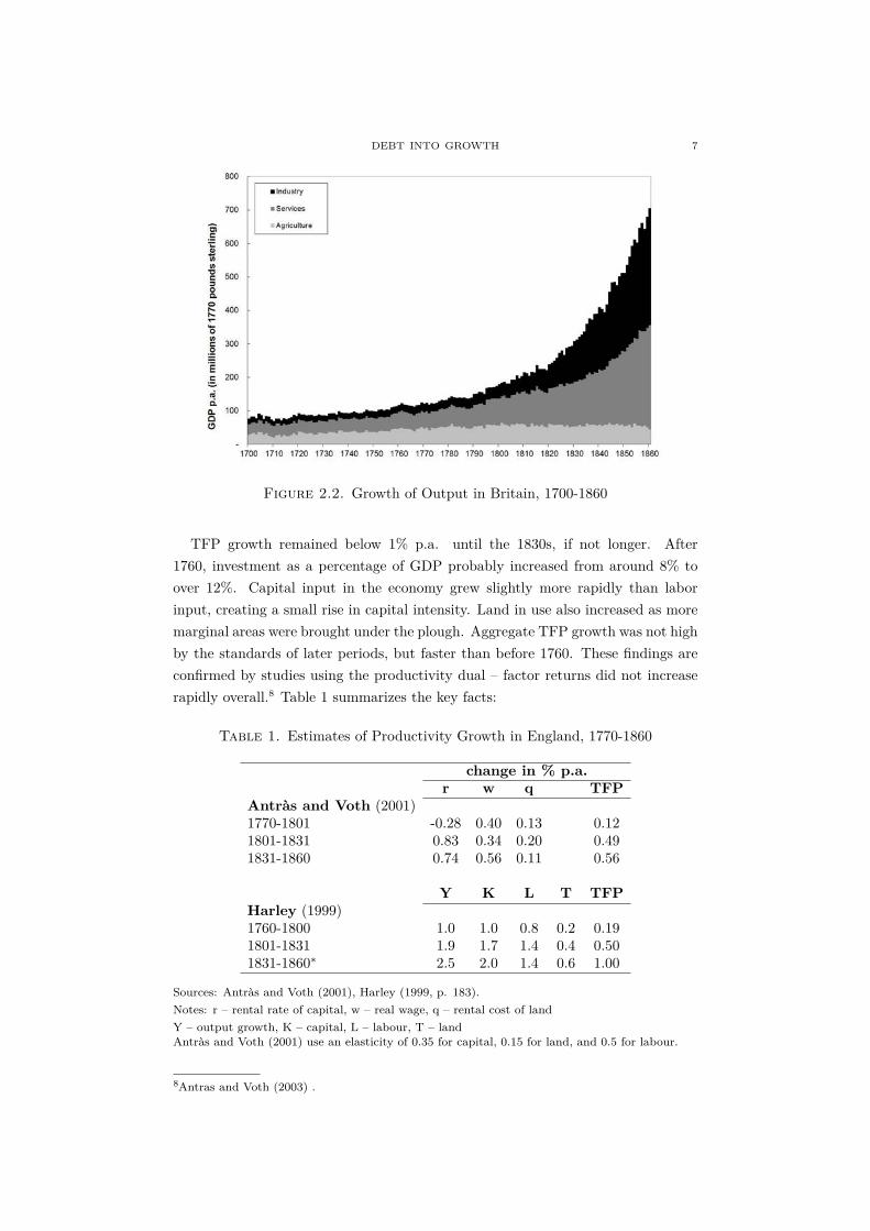
TFP growth remained below 1% p.a. until the 1830s, if not longer. After1760, investment as a percentage of GDP probably increased from around 8% toover 12%. Capital input in the economy grew slightly more rapidly than laborinput, creating a small rise in capital intensity. Land in use also increased as moremarginal areas were brought under the plough. Aggregate TFP growth was not highby the standards of later periods, but faster than before 1760. These findings areconfirmed by studies using the productivity dual – factor returns did not increaserapidly overall.8 Table 1 summarizes the key facts:

Table 1. Estimates of Productivity Growth in England, 1770-1860

change in % p.a.r w q TFP

Antràs and Voth (2001)1770-1801 -0.28 0.40 0.13 0.121801-1831 0.83 0.34 0.20 0.491831-1860 0.74 0.56 0.11 0.56

Y K L T TFPHarley (1999)1760-1800 1.0 1.0 0.8 0.2 0.191801-1831 1.9 1.7 1.4 0.4 0.501831-1860∗ 2.5 2.0 1.4 0.6 1.00

Sources: Antràs and Voth (2001), Harley (1999, p. 183).Notes: r – rental rate of capital, w – real wage, q – rental cost of landY – output growth, K – capital, L – labour, T – landAntràs and Voth (2001) use an elasticity of 0.35 for capital, 0.15 for land, and 0.5 for labour.

8Antras and Voth (2003) .

DEBT INTO GROWTH 8

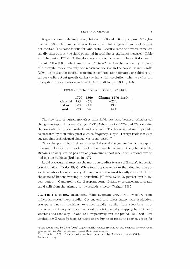
Wages increased relatively slowly between 1760 and 1860, by approx. 30% (Fe-instein 1998). The remuneration of labor thus failed to grow in line with outputper capita.9 The same is true for land rents. Because rents and wages grew lessrapidly than output, the share of capital in total factor payments increased (Table2). The period 1770-1850 therefore saw a major increase in the capital share ofoutput (Allen 2009), which rose from 18% to 45% in less than a century. Growthof the capital stock was only one reason for the rise in the capital share. Crafts(2005) estimates that capital deepening contributed approximately one third to to-tal per capita output growth during the Industrial Revolution. The rate of returnon capital in Britain also grew from 10% in 1770 to over 23% by 1860.

Table 2. Factor shares in Britain, 1770-1860

1770 1860 Change 1770-1860Capital 18% 45% +27%Labor 60% 47% -13%Land 22% 8% -14%

The slow rate of output growth is remarkable not least because technologicalchange was rapid. A “wave of gadgets” (TS Ashton) in the 1770s and 1780s createdthe foundations for new products and processes. The frequency of useful patents,as measured by their subsequent citation frequency, surged. Foreign trade statisticssuggest that technological change was broad-based.10

These changes in factor shares also spelled social change. As income on capitalincreased, the relative importance of landed wealth declined. Slowly but steadily,Britain’s nobility lost its position of paramount importance in the national wealthand income rankings (Rubinstein 1977).

Rapid structural change was the most outstanding feature of Britain’s industrialtransformation (Crafts 1985). While total population more than doubled, the ab-solute number of people employed in agriculture remained broadly constant. Thus,the share of Britons working in agriculture fell from 57 to 25 percent over a 150year period.11 Compared to the ‘European norm’, Britain experienced an early andrapid shift from the primary to the secondary sector (Wrigley 1985).

2.3. The rise of new industries. While aggregate growth rates were low, someindividual sectors grew rapidly. Cotton, and to a lesser extent, iron production,transportation, and machinery expanded rapidly, starting from a low base. Pro-ductivity in cotton production increased by 2.6% annually, shipping by 2.3%, andworsteds and canals by 1.3 and 1.8% respectively over the period 1780-1860. Thisimplies that Britain became 8.8 times as productive in producing cotton goods, for

9More recent work by Clark (2005) suggests slightly faster growth, but still confirms the conclusionthat output growth was markedly faster than wage growth.10Cf. Temin (1997) . The conclusion has been questioned by Crafts and Harley (2000).11Crafts (1985).

DEBT INTO GROWTH 9

Figure 2.3. The growth of modernizing industrial sectors, 1770-1831 (value added in millions of pounds sterling p.a.)

example. Output in new sectors expanded even more, as more labor and capitalwere drawn in. Cotton production increased 42-fold over the period.

As the new sectors grew, their share of the industrial sector increased – and theeconomy itself became increasingly industrialized. Figure 2.3 illustrates the growingimportance of “modernizing” sectors. From 13% of industrial output, modernizingsectors grew to 36% by 1831. In other words, by 1830, more than one third ofindustrial output already came from the sectors that benefited the most from thenew inventions of the industrial era, a share that only increased subsequently.

2.4. The UK financial system. While government debt surged after 1680, pri-vate credit intermediation remained remarkably underdeveloped. As Postan (1935)observed, “the reservoirs of savings were full enough, but conduits to connect themwith the wheels of industry were few and meagre ... surprisingly little of [Britain’s]wealth found its way into the new industrial enterprises ...” . In other words, thenew, dynamic sectors of the economy – cotton manufacturing, iron production, coalmining, ceramics – were initially starved of capital. They largely financed them-selves through retained profits and informal credit. Peer-to-peer lending dominatedwhere credit was available at all – entrepreneurs were forced to turn to friends, fam-ily, and local owners of liquid funds to raise capital (McCraw 1997; Mokyr 1999).12

Private credit markets worked poorly for several reasons. The Bank of Englandwas largely a conduit for government debt. Goldsmith banks were small and few

12In contrast to France, Britain had no system of public notaries who facilitated such transactions(Hoffman, Postel-Vinay, and Rosenthal 2000). Note that informal lending is still common today,both in the developing world and in countries with highly developed capital markets (Azam et al.2001, Townsend 2005).

DEBT INTO GROWTH 10

in number, and only catered to a moneyed and landed elite. Merchant banks fi-nanced foreign trade. Almost no financial institutions attempted to provide fundsfor entrepreneurs.13 Banks were hamstrung by government regulations. The sizeof partnerships in England was limited to six, severely curtailing the size of banks.Usury laws limited (private) interest rates. This rule made lending on anythingbut the best collateral, and to the safest borrowers, unprofitable. Temin and Voth(2008) document how the usury law led to massive distortions in lending. In ad-dition, loans could legally not be made for periods greater than six months. Thismade it hard for borrowers to use funds for illiquid investments. There was nocentral bank, charged with providing liquidity. Existing banks struggled under thethreat of illiquidity, and many floundered because of it.

Nor could new firms easily raise equity on the stock market. As a result of theSouth Sea bubble, the government introduced tight restrictions on the founding ofnew joint stock companies in the form of the so-called “Bubble Act”. The legislationrequired all new joint stock companies to have a royal charter. Effectively, until itsrepeal in the 19th century, the Bubble Act closed the door on all forms of capitalraising via the issuance of new equity (Harris 1994). In combination, private creditintermediation in Britain before the 1820s worked poorly at best. On the whole, itfailed to provide significant funding for new enterprises, which were mostly financedfrom retained earnings. Nothing attests more eloquently to the shortcomings of theUK financial system than the large gap between rates of return on capital investedin manufacturing on the one hand (Allen 2009 ), and the cost of borrowing on theother.

2.5. The market for land. Wealth in England was overwhelmingly held in theform of land. Lindert (1986) estimates that it accounted for 74% of total wealthin 1740. As late as 1875, this share was close to half. Most land was owned bythe nobility and landed gentry. While land could in general be bought and sold,the extent of the land market was relatively limited. In the Middle Ages, outrightownership of land was only possible for the Crown. Gradually, England evolved twoforms of ownership – freehold and leasehold. Freehold property can be transferredfreely and entitles the owner to all rights. Leasehold comes in a bewildering rangeof types, from tenancy at will to leases for life and leases with large entry “fines”and low annual charges. All of these involved the eventual (possible) reversion offull ownership to the freehold owner.

In addition, many noble estates were structured in the form of perpetual trusts.This made it impossible for heirs to sell land outright, thus checking the tendencyof some nobles to overspend, borrow on mortgage, and then have to sell the landto satisfy creditors. Only leases could be agreed for land held in perpetual trusts.

13Brunt (2006) argues that country banks acted like venture capital firms during the BritishIndustrial Revolution. The cases he shows are suggestive, but it is doubtful that this representsan important part of business financing at the time. The analogy with venture capital firms isalso strained, since the upside to the bank was severely limited – at no more than 5%.

DEBT INTO GROWTH 11

This limited the extent to which land could become a widely-traded asset. As aresult, almost no Englishmen other than members of the titled elite could aspireto freeholds. Nor could commoners freely add to land holdings due to a generalscarcity of property available for outright purchase.

In one sense, however, the market for land in England was efficient. Leaseholderspaid rent charges to the freeholder. These could be renegotiated with varyingfrequency. As Clark (2002) demonstrates, rent charges in general moved with theproductivity of land.

2.6. Comparative rates of return. For our argument to hold, comparative ratesof return on assets have to show a particular ordering. Rates of return on investmentin agriculture have to be lower than on government debt; and government debt inturn has to pay less than equity investments available to capitalists, especially thosein the new industries.

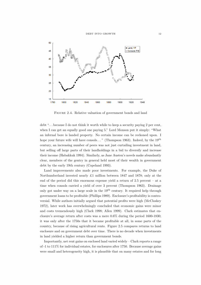
Landlords with money to invest in the land could either acquire more of it (as faras it was available), or use it in improvements such as drainage, liming and marling,as well as enclosure. Neither was more profitable than purchases of governmentbonds. Figure 2.4 shows the relative valuation of government bonds (consols) andof land, from 1795 to 1930. The y-axis measures “year’s purchase”, meaning themultiple of annual payments received by the owner. Until the 1890s, land tradedat a higher multiple than government debt – the interest on the (liquidly traded)debt was markedly higher than the yield on land, which was not only hard to trade;administering it was also costly.

The implications were not lost on landowners. A few, large landholders such asthe Duke of Marlborough had very large holdings of government debt as early as1750 (Dickson 1967). The Earl of Shelburne, at the time of his death in 1751, held99% of his wealth in government debt. Just one generation earlier, this would havebeen unthinkable. Especially newly rich members of the gentry did not commit alarge share of their assets to land anymore:

“Once secure long-term paper assets were available which did notrequire active management by the owner there were very good rea-sons why a new man who wished to establish a landed dynastyshould retain . . . his fortune in such assets. . . as part of the longer-term endowment of the family. They yielded a much higher netincome than that derived from land purchase.”

The Prime Minister, Sir Robert Peel, advised that “every landowner ought to haveas much property (as his estate) in consols or other securities. . . ” (Habakkuk 1994).

Nonetheless, in the mid-eighteenth century, most of the landed elite was yet tomove massively into consols and other government debt. Over the next hundredyears, they did so. The period after 1750 saw an important reduction in investmentsin land and an increase of investments in government debt. As one large landownerexplained to another in 1847, he was going to sell land and invest in government

DEBT INTO GROWTH 12

Figure 2.4. Relative valuation of government bonds and land

debt “. . . because I do not think it worth while to keep a security paying 2 per cent,when I can get an equally good one paying 5.” Lord Monson put it simply: “Whatan infernal bore is landed property. No certain income can be reckoned upon. Ihope your future wife will have consols. . . ” (Thompson 1963). Indeed, by the 19th

century, an increasing number of peers was not just curtailing investment in land,but selling off large parts of their landholdings in a bid to diversify and increasetheir income (Habakkuk 1994). Similarly, as Jane Austen’s novels make abundantlyclear, members of the gentry in general held most of their wealth in governmentdebt by the early 19th century (Copeland 1993).

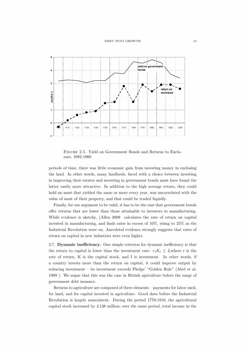
Land improvements also made poor investments. For example, the Duke ofNorthumberland invested nearly £1 million between 1847 and 1878; only at theend of the period did this enormous expense yield a return of 2.5 percent – at atime when consols carried a yield of over 3 percent (Thompson 1963). Drainageonly got under way on a large scale in the 19th century. It required help throughgovernment loans to be profitable (Phillips 1989). Enclosure’s profitability is contro-versial. While authors initially argued that potential profits were high (McCloskey1972), later work has overwhelmingly concluded that economic gains were minorand costs tremendously high (Clark 1998; Allen 1999). Clark estimates that en-closure’s average return after costs was a mere 0.6% during the period 1600-1830;it was only after the 1750s that it became profitable at all, in some parts of thecountry, because of rising agricultural rents. Figure 2.5 compares returns to landenclosure and on government debt over time. There is no decade when investmentsin land yielded a higher return than government bonds.

Importantly, net rent gains on enclosed land varied widely – Clark reports a rangeof -1 to 111% for individual estates, for enclosures after 1750. Because average gainswere small and heterogeneity high, it is plausible that on many estates and for long

DEBT INTO GROWTH 13

Figure 2.5. Yield on Government Bonds and Returns to Enclo-sure, 1692-1860

periods of time, there was little economic gain from investing money in enclosingthe land. In other words, many landlords, faced with a choice between investingin improving their estates and investing in government bonds must have found thelatter vastly more attractive. In addition to the high average return, they couldhold an asset that yielded the same or more every year, was uncorrelated with thevalue of most of their property, and that could be traded liquidly.

Finally, for our argument to be valid, it has to be the case that government bondsoffer returns that are lower than those attainable to investors in manufacturing.While evidence is sketchy, (Allen 2009 calculates the rate of return on capitalinvested in manufacturing, and finds rates in excess of 10%, rising to 25% as theIndustrial Revolution wore on. Anecdotal evidence strongly suggests that rates ofreturn on capital in new industries were even higher.

2.7. Dynamic inefficiency. One simple criterion for dynamic inefficiency is thatthe return to capital is lower than the investment rate: rtKt ≤ Itwhere r is therate of return, K is the capital stock, and I is investment. In other words, ifa country invests more than the return on capital, it could improve output byreducing investment – its investment exceeds Phelps’ “Golden Rule” (Abel et al.1989 ). We argue that this was the case in British agriculture before the surge ofgovernment debt issuance.

Returns to agriculture are composed of three elements – payments for labor used,for land, and for capital invested in agriculture. Good data before the IndustrialRevolution is largely nonexistent. During the period 1770-1810, the agriculturalcapital stock increased by £138 million; over the same period, total income in the

DEBT INTO GROWTH 14

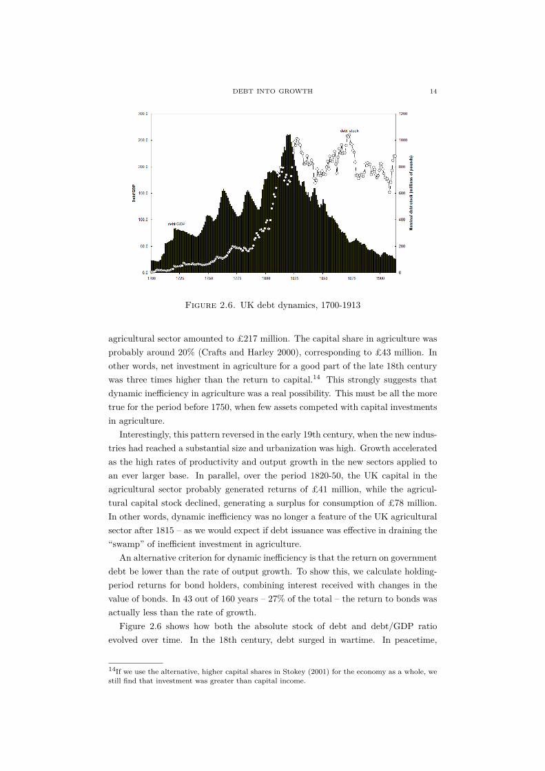
Figure 2.6. UK debt dynamics, 1700-1913

agricultural sector amounted to £217 million. The capital share in agriculture wasprobably around 20% (Crafts and Harley 2000), corresponding to £43 million. Inother words, net investment in agriculture for a good part of the late 18th centurywas three times higher than the return to capital.14 This strongly suggests thatdynamic inefficiency in agriculture was a real possibility. This must be all the moretrue for the period before 1750, when few assets competed with capital investmentsin agriculture.

Interestingly, this pattern reversed in the early 19th century, when the new indus-tries had reached a substantial size and urbanization was high. Growth acceleratedas the high rates of productivity and output growth in the new sectors applied toan ever larger base. In parallel, over the period 1820-50, the UK capital in theagricultural sector probably generated returns of £41 million, while the agricul-tural capital stock declined, generating a surplus for consumption of £78 million.In other words, dynamic inefficiency was no longer a feature of the UK agriculturalsector after 1815 – as we would expect if debt issuance was effective in draining the“swamp” of inefficient investment in agriculture.

An alternative criterion for dynamic inefficiency is that the return on governmentdebt be lower than the rate of output growth. To show this, we calculate holding-period returns for bond holders, combining interest received with changes in thevalue of bonds. In 43 out of 160 years – 27% of the total – the return to bonds wasactually less than the rate of growth.

Figure 2.6 shows how both the absolute stock of debt and debt/GDP ratioevolved over time. In the 18th century, debt surged in wartime. In peacetime,

14If we use the alternative, higher capital shares in Stokey (2001) for the economy as a whole, westill find that investment was greater than capital income.

DEBT INTO GROWTH 15

its level was essentially flat, or falling slightly at best; but debt/GDP ratios de-clined rapidly as growth eroded the relative weight of previous borrowing. Thesame mechanism was at work after 1815. In 1815, after the end of the NapoleonicWars, Britain’s debt amounted to £792 million ; in 1914, to £843 million, some6% higher. At the same time, the debt/GDP ratio declined to 1/10th of its formerlevel, from 226% to 25%. Britain’s 18th century borrowings were never repaid;its massive debts simply dwindled into insignificance as a result of rapid economicgrowth.

3. Debt into growth: understanding the mechanism

Here, we present our argument in four steps. First, we present our basic setupand describe the pre-industrial steady state. Second, we model the Industrial Rev-olution as a process of structural change and show how the absence of an effectiveprivate credit market allows us to account for some of its key historical features.Third, we use the model to study the effects of sovereign debt and the channelsthrough which it affects structural change and economic growth. Fourth, we simu-late the model to gain insight intor the quantitative importance of the mechanismthat we propose.

3.1. The pre-industrial society. Consider an economy with a single or compositegood that is produced with three factors, land, capital and labor. The productiontechnology can be represented as follows:

(3.1) F (lt, kt, nt) = lλt · kαt · n1−λ−αt

where lt, kt and nt are land, capital and labor; and λ > 0, α > 0 and λ+α < 1. Landand labor exist in fixed supply and we normalize their sizes to one, i.e. lt = nt = 1.Capital depreciates at rate δ. To produce one unit of capital in period t + 1, oneunit of goods must be invested in period t. Factor markets are competitive andall factors are paid their marginal products. Owners of land and capital earn afraction λ and α of the output, respectively; while labor earns the rest.

The pre-industrial economy contains two groups, nobles and masses, plus thecrown. The nobles own the land and the capital stock. They save a fraction β oftheir income each period and invest it. The masses own the labor, and they do notsave. The crown fights foreign wars that cost a fraction x of output. We model thiscost as pure waste. In the pre-industrial industrial economy, the crown finances thecost of war with a proportional tax on production which reduces the income of allfactors by a fraction x.

With this simple set of assumptions, we can trace the dynamics of the capitalstock in the pre-industrial economy:

(3.2) kt+1 = (1− δ) · kt + β · (λ+ α) · (1− x) · kαt

Equation (3.2) describes the dynamics of the pre-industrial economy. These dy-namics follow the law of motion of the classic Solow model with an investment rate

DEBT INTO GROWTH 16

equal to β · (λ+ α) · (1− x). From any starting capital stock, the pre-industrialeconomy converges monotonically to a steady state with the following capital stock:

(3.3) k∗ =[β · (λ+ α) · (1− x)

δ

] 11−α

We take the steady state of the pre-industrial economy as the starting point ofour story. From here, we analyze the consequences of two major developments.The first one is the Industrial Revolution which we interpret as the arrival of a newclass of capitalists that brought many important inventions and innovations thatradically transformed the British economy. The second development is the GloriousRevolution that converted Britain into a credible borrower and allowed the crownto finance foreign wars through debt accumulation rather than taxes. We studyeach of these developments in turn.

3.2. A stylized model of the Industrial Revolution. Assume now the arrivalof a new class of capitalists with a new industrial technology and an arbitrarilysmall initial stock of capital. Like the nobles, capitalists save a fraction β of theirincome and invest it. But their technology is π > 1 times more efficient than thatof the nobles. That is, for each unit of goods they invest, they obtain π units ofcapital while the nobles obtain only only one unit.

A reasonable-looking but untrue story for the Industrial Revolution would goas follows. The capitalists had great investment opportunities, while the nobleshad plenty of savings. This situation led to the rapid development of a privatecredit market where capitalists heavily borrowed from nobles. Competition forfunds equalized the interest rate to the return to the capitalists’ investments. Interms of our stylized model, the Industrial Revolution transforms the dynamics ofaccumulation as follows:

(3.4) kt+1 = (1− δ) · kt + π · β · (λ+ α) · (1− x) · kαt

(3.5) st+1 = (1− δ) · kt + π · β · α · (1− x) · kαt(1− δ) · kt + π · β · (λ+ α) · (1− x) · kαt

· st

where st is the share of the capital stock owned by capitalists. Since the capitalistssave the same fraction of their income as the nobles, the aggregate investmentrate is not affected by the Industrial Revolution. But Equation (3.4) shows thatinvestment efficiency is now higher since each unit of goods invested produces πunits of capital rather than one. Equation (3.5) shows how the share of the capitalstock owned by the capitalists evolves over time. To understand this Equation,note that the investment that capitalists finance capitalists finance in period t isβ · α · st · (1− x) · kαt , while total investment is β · (λ+ α) · (1− x) · kαt . Fromany starting capital stock, the industrial economy converges to the following steadystate:

(3.6) k∗ =[π · β · (λ+ α) · (1− x)

δ

] 11−α

and s∗ = 0

DEBT INTO GROWTH 17

0 50 100 150 200 250 300 350 400 450 5000

50

100

150

200

250

300

350

400

450

t

The Capital Stock

K t without Credi t Market

K t with Credi t Market

0 50 100 150 200 250 300 350 400 450 5000

0.2

0.4

0.6

0.8

1

t

The Capital Share of the Capital i sts

st without Credi t Market

st with Credi t Market

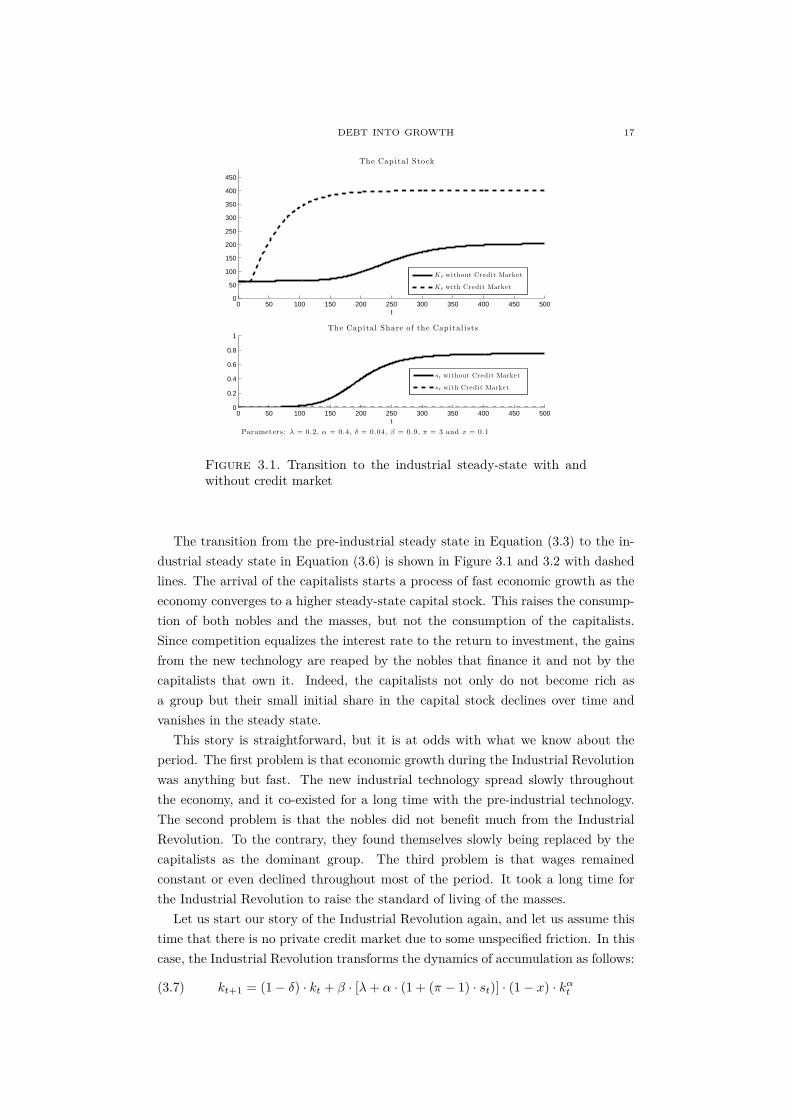
Parameters : λ = 0.2, α = 0.4, δ = 0.04, β = 0.9, π = 3 and x = 0.1

Figure 3.1. Transition to the industrial steady-state with andwithout credit market

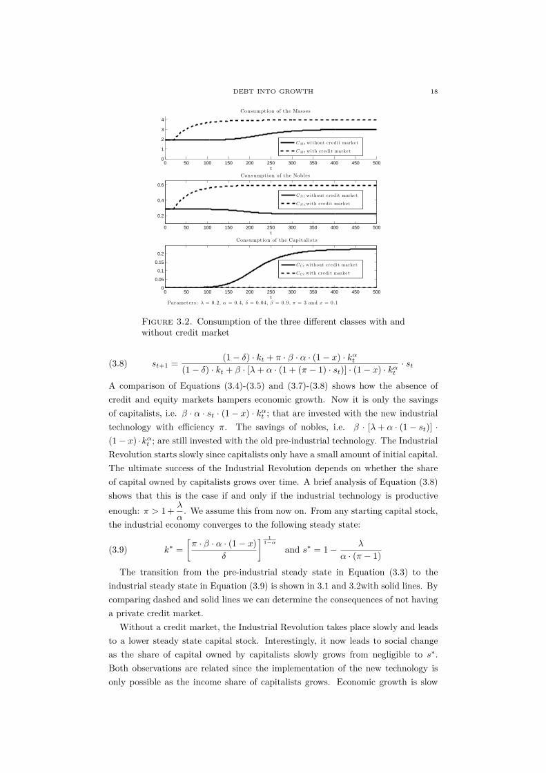
The transition from the pre-industrial steady state in Equation (3.3) to the in-dustrial steady state in Equation (3.6) is shown in Figure 3.1 and 3.2 with dashedlines. The arrival of the capitalists starts a process of fast economic growth as theeconomy converges to a higher steady-state capital stock. This raises the consump-tion of both nobles and the masses, but not the consumption of the capitalists.Since competition equalizes the interest rate to the return to investment, the gainsfrom the new technology are reaped by the nobles that finance it and not by thecapitalists that own it. Indeed, the capitalists not only do not become rich asa group but their small initial share in the capital stock declines over time andvanishes in the steady state.

This story is straightforward, but it is at odds with what we know about theperiod. The first problem is that economic growth during the Industrial Revolutionwas anything but fast. The new industrial technology spread slowly throughoutthe economy, and it co-existed for a long time with the pre-industrial technology.The second problem is that the nobles did not benefit much from the IndustrialRevolution. To the contrary, they found themselves slowly being replaced by thecapitalists as the dominant group. The third problem is that wages remainedconstant or even declined throughout most of the period. It took a long time forthe Industrial Revolution to raise the standard of living of the masses.

Let us start our story of the Industrial Revolution again, and let us assume thistime that there is no private credit market due to some unspecified friction. In thiscase, the Industrial Revolution transforms the dynamics of accumulation as follows:

(3.7) kt+1 = (1− δ) · kt + β · [λ+ α · (1 + (π − 1) · st)] · (1− x) · kαt

DEBT INTO GROWTH 18

0 50 100 150 200 250 300 350 400 450 5000

1

2

3

4

t

Consumpt ion of the Masses

CMt without credi t market

CMt with credi t market

0 50 100 150 200 250 300 350 400 450 500

0.2

0.4

0.6

t

Consumpt ion of the Nobles

CN t without credi t market

CN t with credi t market

0 50 100 150 200 250 300 350 400 450 5000

0.05

0.1

0.15

0.2

t

Consumpt ion of the Capitalis t s

CCt without credi t market

CCt with credi t market

Parameters : λ = 0.2, α = 0.4, δ = 0.04, β = 0.9, π = 3 and x = 0.1

Figure 3.2. Consumption of the three different classes with andwithout credit market

(3.8) st+1 = (1− δ) · kt + π · β · α · (1− x) · kαt(1− δ) · kt + β · [λ+ α · (1 + (π − 1) · st)] · (1− x) · kαt

· st

A comparison of Equations (3.4)-(3.5) and (3.7)-(3.8) shows how the absence ofcredit and equity markets hampers economic growth. Now it is only the savingsof capitalists, i.e. β · α · st · (1− x) · kαt ; that are invested with the new industrialtechnology with efficiency π. The savings of nobles, i.e. β · [λ+ α · (1− st)] ·(1− x) ·kαt ; are still invested with the old pre-industrial technology. The IndustrialRevolution starts slowly since capitalists only have a small amount of initial capital.The ultimate success of the Industrial Revolution depends on whether the shareof capital owned by capitalists grows over time. A brief analysis of Equation (3.8)shows that this is the case if and only if the industrial technology is productiveenough: π > 1 + λ

α. We assume this from now on. From any starting capital stock,

the industrial economy converges to the following steady state:

(3.9) k∗ =[π · β · α · (1− x)

δ

] 11−α

and s∗ = 1− λ

α · (π − 1)

The transition from the pre-industrial steady state in Equation (3.3) to theindustrial steady state in Equation (3.9) is shown in 3.1 and 3.2with solid lines. Bycomparing dashed and solid lines we can determine the consequences of not havinga private credit market.

Without a credit market, the Industrial Revolution takes place slowly and leadsto a lower steady state capital stock. Interestingly, it now leads to social changeas the share of capital owned by capitalists slowly grows from negligible to s∗.Both observations are related since the implementation of the new technology isonly possible as the income share of capitalists grows. Economic growth is slow

DEBT INTO GROWTH 19

due to a misallocation of investment that declines slowly over time and never quitedisappears. That is, economic growth is slow because it requires social change andthe latter happens only slowly.

The absence of a private credit market hurts the nobles and the masses. Bothgroups consume less because capital accumulation slows down. But the nobles arefurther hurt because they cannot appropriate the gains from the new technology,and this reduces their share of this reduced income. The key beneficiaries of theabsence of a private credit market are the capitalists. With a well-functioningprivate credit market, they would have been condemned to a marginal role as thegains from their technology would have been passed on to the nobles. Without awell-functioning credit market, overall growth is initially slower, but the capitalistskeep these gains and their income share increases.

3.3. The role of sovereign debt. Assume now that the arrival of the capitalistscoincides with a shift from taxes to debt. Although the cost of foreign wars remainsa fraction x of output, the crown no longer needs to finance this cost entirely throughtaxes as it can issue debt:

(3.10) dt+1 = Rt · dt + (x− τ) · kαt

where dt are the funds raised by issuing debt in period t−1, Rt is the gross interestrate paid on this debt and τ is taxes as a share of output. Equation (3.10) simplysays that the crown issues new debt to cover interest payments on existing debtplus the costs of foreign wars minus taxes.

If the debt issued does not exceed the savings of the nobles, the crown must payan interest rate that equals the return to the investment of nobles:

(3.11) Rt = (1− τ) · α · kα−1t + 1− δ

At this interest rate, nobles are willing to purchase the crown’s debt. But capitalistsare not willing to do this since the return to their investments is higher: π · (1− τ) ·α · kα−1

t + 1− δ > Rt.For the debt policy described in Equations (3.10) and (3.11) to be feasible, two

assumptions are needed. The first one is that debt dynamics be positive so thattaxes need not be raised to pay for the debt. This requires that π · β > 1. Thesecond assumption is that the total amount of debt never exceeds the wealth ofthe nobles. This requires that x− τ1− τ <

λ

1 + π·(1−β)δ·(π·β−1)

. These two assumptions are

consistent with the evidence presented in section II, and we keep them in whatfollows. Thus, we can now write the dynamics of the industrial economy as follows:(3.12)kt+1 = (1− δ) · kt + β · {[λ+ α · (1 + (π − 1) · st)] · (1− τ) · kαt +Rt · dt} − dt+1

(3.13)

st+1 = (1− δ) · kt + π · β · α · (1− τ) · kαt(1− δ) · kt + β · {[λ+ α · (1 + (π − 1) · st)] · (1− τ) · kαt +Rt · dt} − dt+1

·st

DEBT INTO GROWTH 20

0 50 100 150 200 250 300 350 400 450 5000

50

100

150

200

250

t

The Capital Stock

K t with Debt

K t with Taxes

0 50 100 150 200 250 300 350 400 450 5000

0.2

0.4

0.6

0.8

1

t

The Capital Share of the Capital i sts

st with Debt

st with Taxes

Parameters : λ = 0.2, α = 0.4, δ = 0.04, β = 0.9, π = 3, x = 0.1 and τ = 0.08

Figure 3.3. Transition to the industrial steady-state with debtand taxes

Equation (3.12) shows that, for a given share of the capital stock owned by cap-italists, debt slows down capital accumulation. The reason is that sovereign debtcrowds out investment by the nobles. In particular, their investment declines bydt+1 − β · Rt · dt. But Equation (3.13) also shows that debt increases the shareof capital owned by capitalists. From any starting capital stock, the industrialeconomy converges to the following steady state:

(3.14) k∗ =[π · β · α · (1− τ)

δ

] 11−α

and s∗ = 1−λ− x−τ

1−τ ·[1 + π·(1−β)

δ·(π·β−1)

]α · (π − 1)

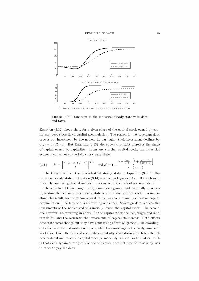
The transition from the pre-industrial steady state in Equation (3.3) to theindustrial steady state in Equation (3.14) is shown in Figures 3.3 and 3.4 with solidlines. By comparing dashed and solid lines we see the effects of sovereign debt.

The shift to debt financing initially slows down growth and eventually increasesit, leading the economy to a steady state with a higher capital stock. To under-stand this result, note that sovereign debt has two countervailing effects on capitalaccumulation. The first one is a crowding-out effect. Sovereign debt reduces theinvestments of the nobles and this initially lowers the capital stock. The secondone however is a crowding-in effect. As the capital stock declines, wages and landrentals fall and the return to the investments of capitalists increase. Both effectsaccelerate social change but they have contrasting effects on growth. The crowding-out effect is static and works on impact, while the crowding-in effect is dynamic andworks over time. Hence, debt accumulation initially slows down growth but then itaccelerates it and raises the capital stock permanently. Crucial for this latter resultis that debt dynamics are positive and the crown does not need to raise surplusesin order to pay the debt.

DEBT INTO GROWTH 21

0 50 100 150 200 250 300 350 400 450 5000

1

2

3

t

Consumpt ion of the Masses

CMt with Debt

CMt with Taxes

0 50 100 150 200 250 300 350 400 450 5000

0.5

1

t

Consumpt ion of the Nobles

CN t with Debt

CN t with Taxes

0 50 100 150 200 250 300 350 400 450 5000

0.1

0.2

0.3

t

Consumpt ion of the Capitalis t s

CCt with Debt

CCt with Taxes

Parameters : λ = 0.2, α = 0.4, δ = 0.04, β = 0.9, π = 3, x = 0.1 and τ = 0.08

Figure 3.4. Consumption of the three different classes with debtand taxes

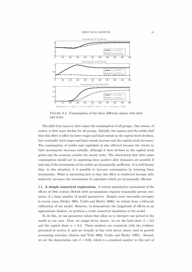
The shift from taxes to debt raises the consumption of all groups. One reason, ofcourse, is that taxes decline for all groups. Initially, the masses and the nobles findthat this effect is offset by lower wages and land rentals as the capital stock declines,but eventually both wages and land rentals increase and the capital stock increases.The consumption of nobles and capitalists is also affected because the return totheir investments increases initially, although it then declines as the capital stockgrows and the economy reaches the steady state. The observation that debt raisesconsumption should not be surprising since positive debt dynamics are possible ifand only if the investments of the nobles are dynamically inefficient. It is well-knownthat, in this situation, it is possible to increase consumption by lowering theseinvestments. What is interesting here is that this effect is reinforced because debtindirectly increases the investments of capitalists which are dynamically efficient.

3.4. A simple numerical exploration. A serious quantitative assessment of theeffects of 18th century British debt accumulation requires reasonably precise esti-mates of a large number of model parameters. Despite some successful attemptsin recent years (Stokey 2001, Crafts and Harley 2000), we refrain from a full-scalecalibration of our model. However, to demonstrate the magnitude of effects in anapproximate fashion, we perform a crude numerical simulation of the model.

To do this, we use parameter values that allow us to interpret one period in themodel as one year. First, we assign factor shares: we set the land share λ = 0.2and the capital share α = 0.4. These numbers are consistent with the evidencepresented in section 2, and are broadly in line with factor shares used in growthaccounting exercises (Antras and Voth 2003, Crafts and Harley 1992). Second,we set the depreciation rate δ = 0.04, which is a standard number in this sort of

DEBT INTO GROWTH 22

exercises. Third, we set the relative efficiency of investment in the new sectorsπ = 3. This choice for π implies that the Industrial Revolution raises steady-stateper capita income by a factor of 1.6. Fourth, we use β = 0.9. Having a high valuefor β is necessary to create the savings that simultaneously financed the IndustrialRevolution and massive debt accumulation – a key feature of the economic andfinancial history of the period (Neal 1993). Finally, we assume the initial share ofthe capital stock owned by capitalists is 0.001, that inital debt is zero, and that theinitial capital stock is at the steady state of the pre-industrial society.

We consider three scenarios. In all of them, we set x = 0.132. This correspondsto the historical average spending for the period 1700-1850. In the first scenario, weuse τ=0.108 which is also the historical average taxes for the same period. Thus,this scenario assumes an annual government deficit of 2.4% that is financed byissuing debt. We refer to this scenario as the baseline scenario. We then constructtwo scenarios in which we set τ = 0.120 and τ = 0.132, respectively. Thus, in thesecounterfactuals the government deficit is reduced to 1.2% and 0% per annum.15

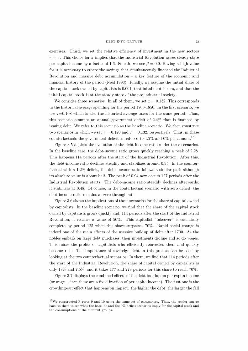
Figure 3.5 depicts the evolution of the debt-income ratio under these scenarios.In the baseline case, the debt-income ratio grows quickly reaching a peak of 2.28.This happens 114 periods after the start of the Industrial Revolution. After this,the debt-income ratio declines steadily and stabilizes around 0.95. In the counter-factual with a 1.2% deficit, the debt-income ratio follows a similar path althoughits absolute value is about half. The peak of 0.94 now occurs 127 periods after theIndustrial Revolution starts. The debt-income ratio steadily declines afterwards;it stabilizes at 0.48. Of course, in the conterfactual scenario with zero deficit, thedebt-income ratio remains at zero throughout.

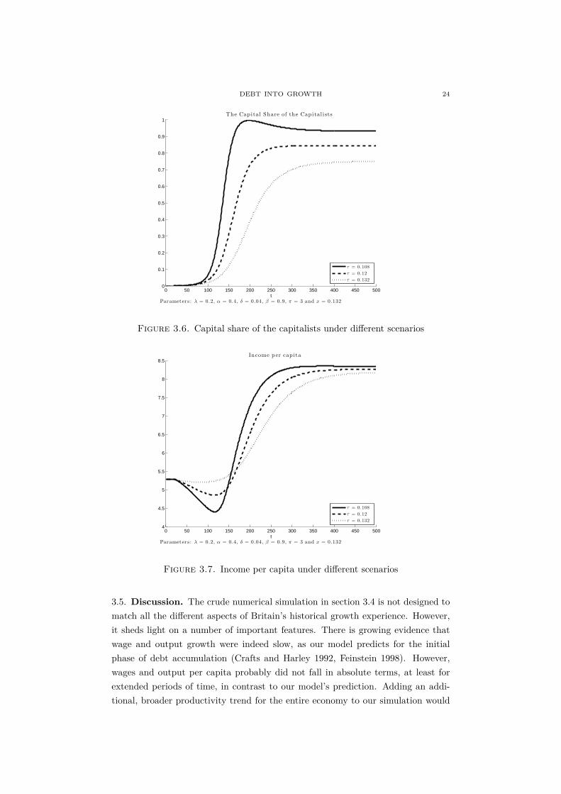
Figure 3.6 shows the implications of these scenarios for the share of capital ownedby capitalists. In the baseline scenario, we find that the share of the capital stockowned by capitalists grows quickly and, 114 periods after the start of the IndustrialRevolution, it reaches a value of 50%. This capitalist ”takeover” is essentiallycomplete by period 125 when this share surpasses 70%. Rapid social change isindeed one of the main effects of the massive buildup of debt after 1700. As thenobles embark on large debt purchases, their investments decline and so do wages.This raises the profits of capitalists who efficiently reinvested them and quicklybecame rich. The importance of sovereign debt in this process can be seen bylooking at the two counterfactual scenarios. In them, we find that 114 periods afterthe start of the Industrial Revolution, the share of capital owned by capitalists isonly 18% and 7.5%; and it takes 177 and 278 periods for this share to reach 70%.

Figure 3.7 displays the combined effects of the debt buildup on per capita income(or wages, since these are a fixed fraction of per capita income). The first one is thecrowding-out effect that happens on impact: the higher the debt, the larger the fall

15We constructed Figures 9 and 10 using the same set of parameters. Thus, the reader can goback to them to see what the baseline and the 0% deficit scenarios imply for the capital stock andthe consumptions of the different groups.

DEBT INTO GROWTH 23

0 50 100 150 200 250 300 350 400 450 5000

0.5

1

1.5

2

2.5

t

Debt-to-Income Ratio

τ = 0.108

τ = 0.12

τ = 0.132

Parameters : λ = 0.2, α = 0.4, δ = 0.04, β = 0.9, π = 3 and x = 0.132

Figure 3.5. Debt-to-income ratio under different scenarios

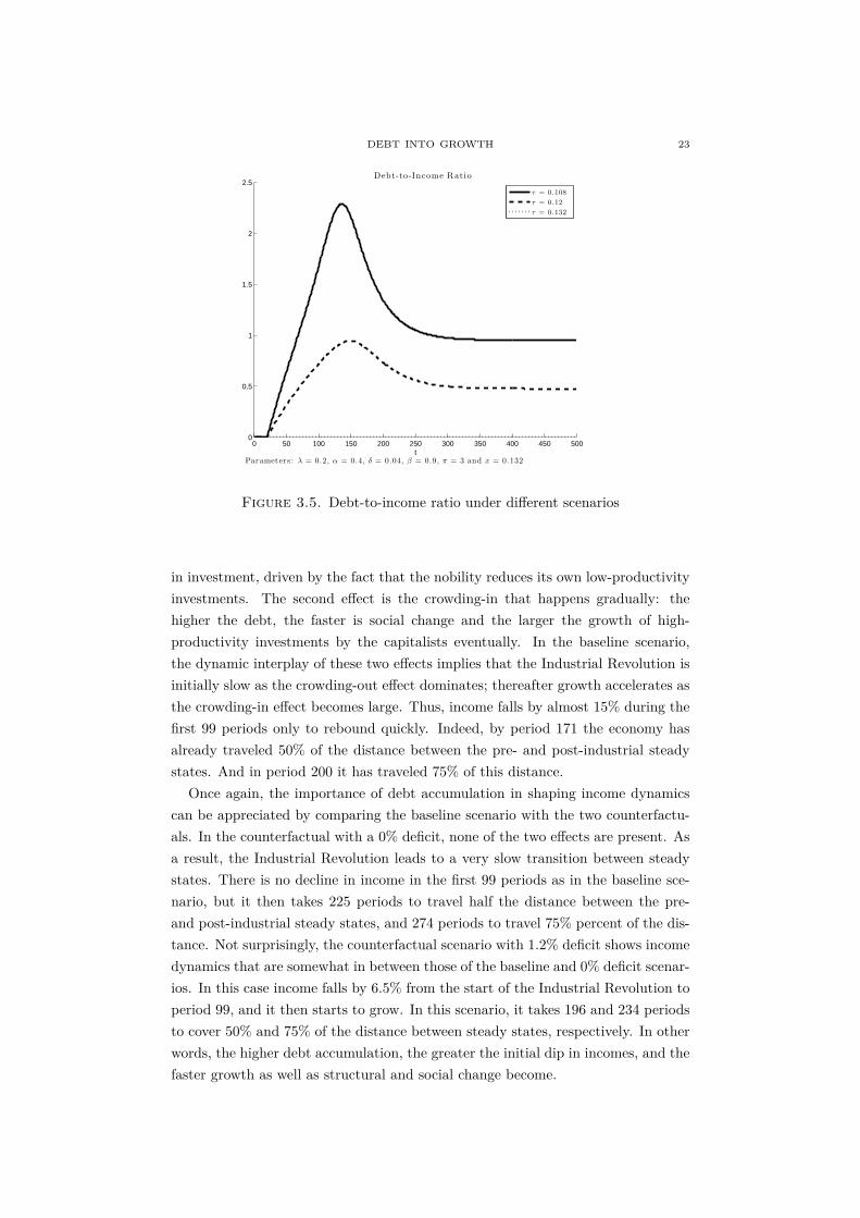
in investment, driven by the fact that the nobility reduces its own low-productivityinvestments. The second effect is the crowding-in that happens gradually: thehigher the debt, the faster is social change and the larger the growth of high-productivity investments by the capitalists eventually. In the baseline scenario,the dynamic interplay of these two effects implies that the Industrial Revolution isinitially slow as the crowding-out effect dominates; thereafter growth accelerates asthe crowding-in effect becomes large. Thus, income falls by almost 15% during thefirst 99 periods only to rebound quickly. Indeed, by period 171 the economy hasalready traveled 50% of the distance between the pre- and post-industrial steadystates. And in period 200 it has traveled 75% of this distance.

Once again, the importance of debt accumulation in shaping income dynamicscan be appreciated by comparing the baseline scenario with the two counterfactu-als. In the counterfactual with a 0% deficit, none of the two effects are present. Asa result, the Industrial Revolution leads to a very slow transition between steadystates. There is no decline in income in the first 99 periods as in the baseline sce-nario, but it then takes 225 periods to travel half the distance between the pre-and post-industrial steady states, and 274 periods to travel 75% percent of the dis-tance. Not surprisingly, the counterfactual scenario with 1.2% deficit shows incomedynamics that are somewhat in between those of the baseline and 0% deficit scenar-ios. In this case income falls by 6.5% from the start of the Industrial Revolution toperiod 99, and it then starts to grow. In this scenario, it takes 196 and 234 periodsto cover 50% and 75% of the distance between steady states, respectively. In otherwords, the higher debt accumulation, the greater the initial dip in incomes, and thefaster growth as well as structural and social change become.

DEBT INTO GROWTH 24

0 50 100 150 200 250 300 350 400 450 5000

0.1

0.2

0.3

0.4

0.5

0.6

0.7

0.8

0.9

1

t

The Capital Share of the Capital i sts

τ = 0.108

τ = 0.12

τ = 0.132

Parameters : λ = 0.2, α = 0.4, δ = 0.04, β = 0.9, π = 3 and x = 0.132

Figure 3.6. Capital share of the capitalists under different scenarios

0 50 100 150 200 250 300 350 400 450 5004

4.5

5

5.5

6

6.5

7

7.5

8

8.5

t

Income per capi ta

τ = 0.108

τ = 0.12

τ = 0.132

Parameters : λ = 0.2, α = 0.4, δ = 0.04, β = 0.9, π = 3 and x = 0.132

Figure 3.7. Income per capita under different scenarios

3.5. Discussion. The crude numerical simulation in section 3.4 is not designed tomatch all the different aspects of Britain’s historical growth experience. However,it sheds light on a number of important features. There is growing evidence thatwage and output growth were indeed slow, as our model predicts for the initialphase of debt accumulation (Crafts and Harley 1992, Feinstein 1998). However,wages and output per capita probably did not fall in absolute terms, at least forextended periods of time, in contrast to our model’s prediction. Adding an addi-tional, broader productivity trend for the entire economy to our simulation would

DEBT INTO GROWTH 25

“fix” this problem; but since we mainly aim at clarifying magnitudes, rather thanmaximizing fit, we abstain from such a modification.

Similarly, factor shares probably shifted during the British IR – Allen’s work(Allen 2009b) strongly suggests that, as population surged, the share of nationalincome going to labor declined, while profits in the new sectors were sky-high. Tokeep our exposition simple, we do not include specifications with shifting factorshares; we note in passing that the extremely high rates of profit in new industriesare a clear sign of misallocation – namely a failure to redeploy more capital in thesectors that used it most efficiently, driven by the shortcomings of Britain’s financialsystem (Banerjee and Munshi 2004).

Finally, we note some limitations of our argument. Undoubtedly, the first-bestfor industrializing Britain would have been a financial system that quickly andcheaply transferred capital from agriculture to the new industries. Growth wouldhave been fastest in this case. Given that financial intermediation was stifled bygovernment intervention, the issuance of debt created a second-best solution – itallowed for a transfer of resources from “old” to “new” industries through linkagesin factor markets. The same appliesto the case of war. Without expensive warsand the debt that they required, growth would have been slower – but if an efficientfinancial system had allowed for the transfer of resources directly, Britain could havegrown even faster, and without a “need” for numerous expensive military conflicts.In other words, it was a particular confluence of factors that allowed Britain to pileup debt at a high rate, creating the largest (sustainable) debt mountain in history,while industrializing at the same time: Given the limitations of its financial system,war helped to mitigate the consequences of inefficient capital allocation by crowdingout inefficient investment.

4. Concluding remarks

Under what conditions is debt growth-enhancing? Reinhart and Rogoff (2009)famously argue that major sovereign debt accumulation tends to be associated withlow growth. But not all debt accumulation episodes are similar. What makes this18th century British episode special is the role of debt as a store of value. In theabsence of a well-developed private credit market, the appearance of a new store ofvalue displaced low-productivity investments and released resources that were usedto finance high-productivity investments. Are there other situations where such amechanism might be at work?

We can think at least of two such scenarios. The financial crisis of 2007-08 andthe long expansion that preceded it have been interpreted by many as the result ofan asset bubble popping-up and bursting. Just like sovereign debt, asset bubblesare stores of value. In a similar spirit to ours, a number of recent studies havefocused on how asset bubbles can overcome financial frictions and enhance growth(Caballero and Krishnamurty 2006 , Farhi and Tirole 2014, Martin and Ventura

DEBT INTO GROWTH 26

2014).16 Since 21st century United States and Europe possess developed financialmarkets, this research has emphasized liquidity or collateral, factors that are lesslikely to have played the main role in 18th century Britain.

Factors what we highlight for the case of Britain may also have contributedto China’s spectacular rise in recent decades. Song, Storesletten and Zilibotti(2011) argue that Chinese growth is driven by the transfer of resources from low-productivity state firms to high-productivity private firms – severe financial fric-tions stop private firms from borrowing and force them to finance their investmentsthrough retained earnings. In such a setting, China’s foreign reserve accumulationmay have played a role similar to the buying of government debt by the Britishnobility: Reduced investments by state firms might have lowered the demand forlabor and wages, raising the profits of private firms and leading to faster growthand more rapid structural change.

References

Abel, A. B., N. G. Mankiw, L. H. Summers, and R. J. Zeckhauser (1989):“Assessing Dynamic Efficiency: Theory and Evidence,” The Review of EconomicStudies, 56(1), 1–19.

Allen, R. C. (1999): “Tracking the Agricultural Revolution in England,” TheEconomic History Review, 52(2), pp. 209–235.

(2009a): The British Industrial Revolution in Global Perspective. Cam-bridge University Press.

(2009b): “Engels’ Pause: Technical Change, Capital Accumulation, andInequality in the British Industrial Revolution,” Explorations in Economic His-tory, 46(4), 418 – 435.

Antras, P., and H.-J. Voth (2003): “Factor Prices and Productivity Growthduring the British Industrial Revolution,” Explorations in Economic History,40(1), 52–77.

Ashton, T. S. (1948): The Industrial Revolution 1760-1830, Volume 204. CUPArchive.

Azam, J. P., B. Biais, M. Dia, and C. Maurel (2001): “Informal and Formalcredit markets and credit rationing in Côte d’Ivoire,” Oxford Review of EconomicPolicy, 17(4), 520–534.

Banerjee, A., and K. Munshi (2004): “How efficiently is capital allocated? Ev-idence from the knitted garment industry in Tirupur,” The Review of EconomicStudies, 71(1), 19–42.

Banerjee, A. V., and E. Duflo (2005): “Growth theory through the lens ofdevelopment economics,” Handbook of economic growth, 1, 473–552.

16One exception is Ventura (2012) who shows how asset bubbles reduce the effects of frictions tointernational capital flows by shifting investments from low- to high-productivity countries. Themechanism has a number of similarities with the one we emphasize here, but it works through thecost of capital rather than through wages.

DEBT INTO GROWTH 27

Banerjee, A. V., and E. Duflo (2014): “Do Firms Want to Borrow More?Testing Credit Constraints Using a Directed Lending Program,” The Review ofEconomic Studies, 81(2), 572–607.

Banerjee, A. V., and B. Moll (2010): “Why Does Misallocation Persist?,”American Economic Journal: Macroeconomics, 2(1), 189–206.

Barro, R. J. (1987): “Government Spending, Interest Rates, Prices, and BudgetDeficits in the United Kingdom, 1701-1918,” Journal of Monetary Economics,20(2), 221 – 247.

Brewer, J. (1990): The Sinews of Power? War, Money and the English State,1688-1783. Harvard University Press.

Broadberry, S. N., B. M. Campbell, A. D. Klein, M. Overton, and B. v.Leeuwen (2010): “British Economic Growth: 1270-1870,” Warwick wp.

Brunt, L. (2006): “Rediscovering Risk: Country Banks as Venture Capital Firmsin the First Industrial Revolution,” The Journal of Economic History, 66(01),74–102.

Caballero, R. J., and A. Krishnamurthy (2006): “Bubbles and Capital FlowVolatility: Causes and Risk management,” Journal of Monetary Economics,53(1), 35–53.

Clark, G. (1998): “Commons Sense: Common Property Rights, Efficiency, andInstitutional Change,” The Journal of Economic History, 58(1), pp. 73–102.

(2001): “Debt, Deficits, and Crowding Out: England, 1727-1840,” Euro-pean Review of Economic History, 5(03), 403–436.

(2002): “Land Rental Values and the Agrarian Economy: England andWales, 1500 1914,” European Review of Economic History, 6(03), 281–308.

(2005): “The Condition of the Working Class in Egland, 1209–2004,”Journal of Political Economy, 113(6), 1307–1340.

Crafts, N. (1985): British Economic Growth during the Industrial Revolution.Oxford Clarendon Press.

Crafts, N. (2005): “The First Industrial Revolution: Resolving the SlowGrowth/Rapid Industrialization Paradox,” Journal of the European EconomicAssocation, 3(2/3), 525–534.

Crafts, N. F. R., and C. K. Harley (1992): “Output Growth and the BritishIndustrial Revolution: A Restatement of the Crafts-Harley View,” The EconomicHistory Review, 45(4), pp. 703–730.

Dickson, P. G. M. (1967): The Financial Revolution in England: A Study in theDevelopment of Public Credit, 1688-1756. Macmillan.

Farhi, E., and J. Tirole (2011): “Bubbly liquidity,” The Review of EconomicStudies, p. rdr039.

Feinstein, C. H. (1998): “Pessimism Perpetuated: Real Wages and the Standardof Living in Britain during and after the Industrial Revolution,” The Journal ofEconomic History, 58(3), pp. 625–658.

DEBT INTO GROWTH 28

Galor, O. (2005): “From Stagnation to Growth: Unified Growth Theory,” inHandbook of Economic Growth, ed. by P. Aghion, and S. Durlauf, vol. 1 of Hand-book of Economic Growth, chap. 4, pp. 171–293. Elsevier.

Gancia, G., and F. Zilibotti (2009): “Technological Change and the Wealth ofNations,” Annual Review of Economics, 1(1), 93–120.

Habakkuk, H. J. (1994): Marriage, Debt, and the Estates System: EnglishLandownership, 1650-1950. Clarendon Press.

Harley, C. K., and N. F. Crafts (2000): “Simulating the Two Views of theBritish Industrial Revolution,” The Journal of Economic History, 60(03), 819–841.

Harris, R. (1994): “The Bubble Act: Its Passage and Its Effects on BusinessOrganization,” The Journal of Economic History, 54(3), pp. 610–627.

Heim, C. E., and P. Mirowski (1987): “Interest Rates and Crowding-Out DuringBritain’s Industrial Revolution,” The Journal of Economic History, 47, 117–139.

Hsieh, C.-T., and P. J. Klenow (2009): “Misallocation and Manufacturing TFPin China and India,” The Quarterly Journal of Economics, 124(4), 1403–1448.

Lindert, P. H. (1986): “Unequal English Wealth since 1670,” Journal of PoliticalEconomy, 94(6), pp. 1127–1162.

Martin, A., and J. Ventura (forthcoming): “Managing Credit Bubbles,” Jour-nal of the European Economic Association.

McCloskey, D. N. (1972): “The Enclosure of Open Fields: Preface to a Study ofIts Impact on the Efficiency of English Agriculture in the Eighteenth Century,”The Journal of Economic History, 32(1), pp. 15–35.

McCraw, T. K. (1997): Creating Modern Capitalism: How Entrepreneurs, Com-panies and Countries Triumphed in Three Industrial Revolutions. Harvard Uni-versity Press.

Mirowski, P. (1981): “The Rise (and Retreat) of a Market: English Joint StockShares in the Eighteenth Century,” The Journal of Economic History, 41(3), pp.559–577.

Mokyr, J. (1999): Editor’s Introduction: The New Economic History and TheIndustrial Revolution. Boulder: Westview Press.

Neal, L. (1993): The rise of financial capitalism: International capital markets inthe age of reason. Cambridge University Press.

North, D. C., and B. R. Weingast (1989): “Constitutions and commitment:the evolution of institutions governing public choice in seventeenth-century Eng-land,” The journal of economic history, 49(04), 803–832.

Philip Hoffman, G. P.-V., and J.-L. Rosenthal (2000): Priceless Markets:The Political Economy of Credit in Paris, 1660-1870. University of Chicago Press.

Phillips, A. D. M. (1989): The Underdraining of Farmland in England duringthe Nineteenth Century. Cambridge University Press.

Postan, M. M. (1935): “Recent Trends in the Accumulation of Capital,” TheEconomic History Review, 6(1), pp. 1–12.

DEBT INTO GROWTH 29

Quinn, S. (2001): “The Glorious Revolution’s Effect on English Private Finance: AMicrohistory, 1680-1705,” The Journal of Economic History, 61(3), pp. 593–615.

Reinhart, C. M., and K. Rogoff (2009): This time is different: eight centuriesof financial folly. princeton university press.

Rubinstein, W. D. (1977): “Wealth, Elites and the Class Structure of ModernBritain,” Past and Present, (76), pp. 99–126.

Song, Z., K. Storesletten, and F. Zilibotti (2011): “Growing Like China,”American Economic Review, 101(1), 196–233.

Stokey, N. L. (2001): “A quantitative model of the British industrial revolution,1780–1850,” in Carnegie-Rochester Conference Series on Public Policy, vol. 55,pp. 55–109. Elsevier.

Sussman, N., and Y. Yafeh (2004): “Constitutions and Commitment: Evidenceon the Relation Between Institutions and the Cost of Capital,” CEPR DiscussionPapers 4404, C.E.P.R. Discussion Papers.

(2006): “Institutional reforms, financial development and sovereign debt:Britain 1690–1790,” The Journal of Economic History, 66(04), 906–935.

Temin, P. (1997): “Two Views of the British Industrial Revolution,” The Journalof Economic History, 57(01), 63–82.

Temin, P., and H.-J. Voth (2008): “Interest Rate Restrictions in a NaturalExperiment: Loan Allocation and the Change in the Usury Laws in 1714,” TheEconomic Journal, 118(528), pp. 743–758.

Thompson, F. M. L. (1963): English Landed Society in the Nineteenth Century.London: Routledge and Kegan Paul.

Townsend, R. (2005): “Networks and finance in poor neighborhoods,” CreditMarkets for the Poor. New York, NY: Russell Sage Foundation.

Ventura, J. (2012): “Bubbles and capital flows,” Journal of Economic Theory,147(2), 738–758.

Williamson, J. G. (1984): “Why Was British Growth So Slow During the Indus-trial Revolution?,” The Journal of Economic History, 44(3), pp. 687–712.

Wrigley, E. A. (1985): “Urban Growth and Agricultural Change: England andthe Continent in the Early Modern Period,” The Journal of InterdisciplinaryHistory, 15(4), pp. 683–728.