U.U.D.M. Project Report 2016:5

Examensarbete i matematik, 30 hpHandledare: Maciej Klimek Examinator: Erik EkströmApril 2016

Department of MathematicsUppsala University

Debit Value Adjustment & Funding Value Adjustment

Pierre Serti & Tom William

Debit Value Adjustment & FundingValue Adjustment

Pierre Serti & Tom William

A thesis presented for the degree ofMaster of Science in Financial Mathematics

Supervisor: Maciej KlimekDepartment of Mathematics

Uppsala University2016

AbbreviationsBPS Basis Points

CCP Central Counterparty Clearing House

CCR Counterparty Credit Risk

CDF Cumulative Distribution Function

CDS Credit Default Swap

CSA Credit Support Annex

CVA Credit Value Adjustment

DVA Debit Value Adjustment

EAD Exposure At Default

EQD Equity Derivatives

EURIBOR Euro Interbank Offered Rate

FRA Forward Rate Agreement

FVA Funding Value Adjustment

IFRS International Financial Reporting Standards

IRS Interest Rate Swap

LGD Loss Given Default

LIBOR London Interbank Offered Rate

LVA Liquidity Value Adjustment

LTCM Long Term Capital Management

MtM Mark-to-Market

OTC Over The Counter

P&L Profit and Loss Statement

PD Probability of Default

PDF Probability Density Function

PV Present Value

R Recovery Rate

Repo Repurchase Agreement

STF Structured Finance Transactions

1

AbstractRecognizing the growing importance of the Debit Value Adjustment (DVA) andthe Funding Value Adjustment (FVA), there are several challenges to imple-menting the DVA and the FVA, not least since there is no standard definitionfor these valuation adjustments as of today. Moreover, due to the fact that thereis no commonly agreed method of how to price these, there are no market con-sensus nor regulatory guidelines on accurate approaches to compute the DVAand the FVA, which leaves the vast banks with this challenging and demandingtask. This paper considers different approaches when pricing DVA and FVA,which stems from different authors in the financial industry. Furthermore, wewill provide a comprehensive overview of both the implications and drawbacksfor the valuation adjustments with respect to double counting, hedging strate-gies and its inclusion on a balance sheet. By not considering DVA and FVAwould leave any bank behind the market and at a disadvantage to the banksthat have adopted these valuation adjustments.

2

AcknowledgementsWe would like to express our sincere appreciation to Prof. Maciej Klimek at theDepartment of Mathematics at Uppsala University for his engaged supervision ofthis thesis and useful advice along the way. Prof. Klimek has with his expertisebeen given us invaluable guidance through challenging moments during thisthesis, none of this would be possible without him. We would also like to thankHåkan Edström at Swedbank LC&I within Valuation Group for his engagementin arranging this master thesis as a project within the bank and his inputsregarding our field of study.Finally, we would also like to thank Jesus Christ and our families for giving usstrength and faith in everything we do.

3

Contents

1 Introduction 61.1 Thesis demarcation . . . . . . . . . . . . . . . . . . . . . . . . . . 61.2 The Swap Market . . . . . . . . . . . . . . . . . . . . . . . . . . . 7

1.2.1 Interest Rates Derivatives . . . . . . . . . . . . . . . . . . 81.2.2 Credit Default Swaps . . . . . . . . . . . . . . . . . . . . 8

1.3 Introduction to Credit Risk . . . . . . . . . . . . . . . . . . . . . 101.4 Counterparty Credit Risk . . . . . . . . . . . . . . . . . . . . . . 11

2 Derivatives 132.1 Exchange-traded derivatives . . . . . . . . . . . . . . . . . . . . . 132.2 OTC Derivatives . . . . . . . . . . . . . . . . . . . . . . . . . . . 142.3 Derivation of the pricing formula . . . . . . . . . . . . . . . . . . 152.4 Derivative Transactions . . . . . . . . . . . . . . . . . . . . . . . 17

2.4.1 OTC derivative schedule . . . . . . . . . . . . . . . . . . . 182.4.2 Exchange traded derivative schedule . . . . . . . . . . . . 19

3 Credit Risk Relationships 203.1 Loss Given Default . . . . . . . . . . . . . . . . . . . . . . . . . . 203.2 Exposure . . . . . . . . . . . . . . . . . . . . . . . . . . . . . . . 223.3 Netting . . . . . . . . . . . . . . . . . . . . . . . . . . . . . . . . 223.4 Netting Agreements . . . . . . . . . . . . . . . . . . . . . . . . . 233.5 Trading Relationship under ISDA Master Agreement . . . . . . . 243.6 Trading Relationship under Collateralization and CSA . . . . . . 25

4 Valuation Adjustments 284.1 XVAs . . . . . . . . . . . . . . . . . . . . . . . . . . . . . . . . . 28

4.1.1 CVA − Credit Valuation Adjustment . . . . . . . . . . . 284.1.2 DVA − Debit Valuation Adjustment . . . . . . . . . . . . 304.1.3 FVA − Funding Value Adjustment . . . . . . . . . . . . . 324.1.4 Double Counting of FVA and DVA . . . . . . . . . . . . . 33

5 DVA on the Balance Sheet 375.1 DVA’s treatment in banks’ balance sheets . . . . . . . . . . . . . 37

4

6 Introduction to Funding Cost 436.1 Pricing of the Derivative subject to the funding cost . . . . . . . 436.2 Pricing of non-collateralized derivatives . . . . . . . . . . . . . . 47

7 First-Hitting Time 527.1 Probability of Default - 1 dimensional . . . . . . . . . . . . . . . 537.2 Probability of Default - Multidimensional . . . . . . . . . . . . . 57

8 Funding Strategies for XVAs 618.1 Set-up prior to semi-replication and pricing . . . . . . . . . . . . 618.2 Semi-replication and pricing . . . . . . . . . . . . . . . . . . . . . 62

9 Conclusion 67

5

Chapter 1

Introduction

1.1 Thesis demarcationRecent financial crisis has lead to new behaviour of the financial system, normsthat previously were neglected in the pre financial crisis has now been treatedand adjusted in order to enhance the stability of the derivative markets. Banksand other financial participants on the Over-The-Counter (OTC) market usuallythought, as they were too big to fail, which gave rise to persisted consequences.Furthermore, this has raised the awareness of mitigating the risk embedded inthe financial market where financial regulators enforce stricter regulations, suchas Basel II and Basel III. In order to avoid potential future losses it is essentialfor banks and other financial institutions to identify and quantify risk. SeveralValuation Adjustments to the OTC derivative contracts have been establishedto be essential and more important than ever before in the credit crisis in thepost Lehman Brothers crash for the whole financial industry.

Recognizing the growing importance of debit value adjustment (DVA) and fund-ing value adjustment (FVA), this paper is designed to investigate the differentapproaches undertaken by the vast financial institutions to implement and pricethe DVA and the FVA. Currently there is no standard definition for these valua-tion adjustments as of yet and hence the many obstacles for financial institutionswhen calibrating DVA and FVA whilst carrying out the credit risk since someof them do not agree on how to manage these as of the several different calcu-lations among different institutions.

We will do our best in providing a thorough and a comprehensive overviewfor the different concepts involved in the DVA and the FVA together with pric-ing techniques that previously have been developed and published by otherresearchers within this field of research and eventually summarize and comparethe different methods established.

6

1.2 The Swap MarketWhen entering into a swap agreement the actual setup refers to letting twoentities swap cash flows with one another. The swap does not take any initialmonetary transactions into consideration. This makes it more desirable for bothparties, as transaction fees do not apply, nor do limitations in terms of bindingcapital.

Swap agreements can involve any type of cash flow. The main purpose of enter-ing into a swap is to exchange a floating cash flow with an inherent risk (highor low) for either a similar cash flow but with a different risk profile, or morelikely a fixed cash flow.

It is important to bear in mind that, when entering into such a swap con-tract, both cash flows in the contractual agreement have a fair setup for bothparties, i.e. the same expected net present value (NPV). All else being equal,the initial value of the contract will always be zero when being entered.

Nowadays it is unorthodox to trade swaps directly between two parties, un-less both parties are financial institutions. Swaps are therefore most likely tobe traded over the counter (OTC) through an intermediary. Generally, an in-termediary is intended to be on the opposite side of the transaction of the swapagreement, while also finding peers to match and cover for the defaulting coun-terparties in such agreement. According to [6] the spread inherent in the swapagreement serves the function of covering for the default risk involved in thecounterparties managed by the intermediary.

Commonly, the intermediary involved in such agreements will have an entireportfolio of entities that currently are in a swap agreement with one another.There may be several tools for mitigating the risk at the intermediary’s disposalarising from the event of default that any of the involved counterparties wouldsuffer from on the financial intermediary’s liabilities.

7

1.2.1 Interest Rates DerivativesThe most common and most frequently-used type of traded swap is the interestrate swap (IRS), where the parties involved agree exchange payment streams ona notional amount. There are several types of IRS, such as Fixed-to-FloatingIRS and Fixed-to-Fixed IRS. However, the most liquid and commonly-used IRSby the financial market is the Fixed-to-Floating, which is also called the plainvanilla IRS.

The parties involved in such an agreement are either called the Receiver (theparty who pays a floating interest rate to the other party) or the party calledthe Payer, i.e. whom ought to pay back the fixed interest rate in question tothe Receiver.

The NPV of the fixed cash flow in a plain vanilla IRS is called the fixed leg, whilethe expected NPV of the floating cash flow is called the floating leg [13]. Thefloating leg of the IRS is typically linked to three- or six-month LIBOR rates,but can also follow any other interest rate index, e.g. three months EURIBOR.

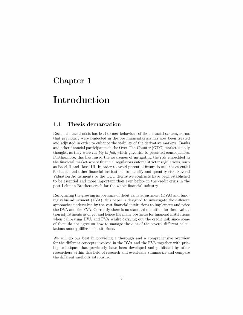
1.2.2 Credit Default SwapsAnother type of swap playing in the majors when it comes to popularity andimportance in the credit derivative market is the credit default swap (CDS),where the swap acts as an insurance policy in the event of default risk. Itprovides insurance against the default of an issuer (the reference credit) or ona specific underlying bond (the reference security). The standard approach insuch agreement is illustrated in the figure below.

The protection buyer pays an annual or a semiannual premium until the eventof either the expiry of the contract or default on the reference entity - whicheveroccurs first. In the event of a default, the protection seller compensates theprotection buyer for the possible loss on the underlying bond.

8

Figure 1.1: An illustration of a CDS agreement in its most basic form betweena protection buyer and a protection seller whereas the protection seller hedgesagainst the credit risk inherent originated from the reference entity 1. Basispoints are used as a measure to describe the percentage change in the value ofinterest rates, e.g. a decrease by 25 basis points means that the interest havedecreased by 0.25%.

There is no doubt that CDS has in the last decade become one of the mostimportant instruments, in fact this is mainly due to usefulness in assessing thecredit risk of a company. The premium rate of such contracts is denoted bytheir respective CDS spreads, which are noted transparently and publicly forfinancial institutions and bigger corporations.

Subject to this assessment, we want to highlight a remarkable event in thehistorical data of CDS spreads, which were considered to be higher than normalprior to the financial crisis as shown below in Figure 1.2. The figure illustratesthe CDS-spreads of five large Banks (Goldman Sachs, Bank of America, SociétéGénérale, Lloyds and Deutsche), which had its first turbulent move in mid 2007with a clear peak around March 2008 originated from the acquisition of BearStearns by JP Morgan.

1http://www.isdacdsmarketplace.com/about_cds_market/how_cds_work

9

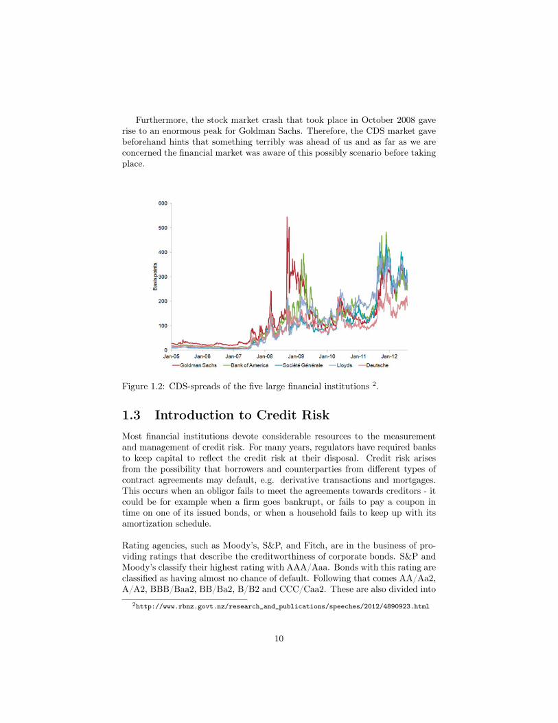
Furthermore, the stock market crash that took place in October 2008 gaverise to an enormous peak for Goldman Sachs. Therefore, the CDS market gavebeforehand hints that something terribly was ahead of us and as far as we areconcerned the financial market was aware of this possibly scenario before takingplace.

Figure 1.2: CDS-spreads of the five large financial institutions 2.

1.3 Introduction to Credit RiskMost financial institutions devote considerable resources to the measurementand management of credit risk. For many years, regulators have required banksto keep capital to reflect the credit risk at their disposal. Credit risk arisesfrom the possibility that borrowers and counterparties from different types ofcontract agreements may default, e.g. derivative transactions and mortgages.This occurs when an obligor fails to meet the agreements towards creditors - itcould be for example when a firm goes bankrupt, or fails to pay a coupon intime on one of its issued bonds, or when a household fails to keep up with itsamortization schedule.

Rating agencies, such as Moody’s, S&P, and Fitch, are in the business of pro-viding ratings that describe the creditworthiness of corporate bonds. S&P andMoody’s classify their highest rating with AAA/Aaa. Bonds with this rating areclassified as having almost no chance of default. Following that comes AA/Aa2,A/A2, BBB/Baa2, BB/Ba2, B/B2 and CCC/Caa2. These are also divided into

2http://www.rbnz.govt.nz/research_and_publications/speeches/2012/4890923.html

10

subcategories by the rating agencies (such as A+, A, A-, or A1, A2, A3). Onlybonds with ratings of BBB/Baa or above are considered to be in an investmentgrade. Each rating is related to the probability of default; a higher rating indi-cates a lower probability of default. The ratings describe the risk premium thatis added to the interest rate of a loan or a bond issued by an entity [7]. Creditrisk is something that is not static, since it can vary over time therefore shoulda company fall below a certain credit rating, its grade changes from investmentquality to high yield status. High yield bonds are the debt of companies in sometype of financial difficulty and due to their riskiness, they potentially have tooffer much higher yields. The last statement tells us that all bonds are not bydefault inherently safer than regular stocks.

1.4 Counterparty Credit RiskCounterparty credit risk (CCR) has gained substantial emphasis in recent years,mostly due to the credit crisis in 2007. Counterparty credit risk is the particularrisk that a counterparty in a derivatives transaction will default prior to thematurity of a trade, and will not thus be able to fulfill its future obligations andpayments, as required by the terms of the contract. Typically, the positionsgiving rise to CCR can be divided into two broad classes of financial products:

• OTC (over the counter) derivatives, e.g. interest rate swaps, FX forwards,credit default swaps

• STF (security financing transactions), e.g. repos, securities borrowing andlending.

The first of these is considered to be more risky than the latter, mainly due tothe rapidly growth and size of the OTC derivative market in recent years andthe diversity of complex OTC derivatives instruments [6].

Article [12] states that there are two features that differentiate counterpartycredit risk from more traditional forms of credit risk. The first particularity ofcounterparty credit risk is the bilateral nature of the credit risk:

A derivate position is built in such way that it has both a positive market valuefor one party and a negative market value for the respective counterparty, butduring the lifetime of the derivative contract, the market value of the contractcan change such that the markets values to each party are now the opposite.Therefore, the presence of credit risk is now a factor for both sides of the con-tract.

Consider an IRS where both parties face credit risk. The contract has a positivemarket value for the fixed payer in the event that the floating rate is above theswap rate, and when the rates have an inverse relation the floating payer is saidto have a positive value in his book. This is however not applicable to a bond,

11

due to the inability of the market value to change as the party holding a longposition faces the entire risk of the issuer defaulting, and therefore bears thecredit risk.

The second cause of counterparty credit risk is the variability in exposure. Theexposure corresponds to how big a proportion of the capital is at risk. By deter-mining the exposure, one can quantify the credit risk of holding a bond position,which is in fact the PV of the bond and also by weighting it with probabilityof the issuer defaulting. We will later on address, a more robust explanation tothe concept of exposure, see section 3.2.

12

Chapter 2

Derivatives

In this chapter we will go through the fundamentals behind exchange-tradedderivatives and OTC derivatives and describe the basic techniques of OTCderivatives. Furthermore, we will derive the classical pricing formula of a deriva-tive written on a an asset and sum up the chapter by displaying the process ofa typical transaction schedule of an exchange traded derivative and and whentraded OTC.

2.1 Exchange-traded derivativesAn exchange-traded derivative is an instrument whose value is based on the valueof another asset class and which is further traded on a regulated exchange. Dueto its advantageous characteristics such as standardization and elimination ofdefault risk, an exchange-traded derivative is hence not affected nor subject tocounterparty risk since the exchange will most likely have a clearing entity totake on that role. Therefore, exchange-traded derivatives provide a market placewhere transparency is featured, and coupled with liquidity being facilitated [6].As an example, if we consider trading a futures contract (an exchange-tradedderivative) the only and tangible counterparty to the futures contract is theexchange itself. Thus, the underlying risk of not receiving the promised cashflows is quite low, since it depends on the survival of the exchange, and notthat of a single counterparty [12]. Due to the need for customization and thedemand for more complex structures of derivatives, a much more significantnotional amount of derivatives are traded over the counter.

13

2.2 OTC DerivativesThe OTC derivative market is by far the largest market for derivatives, coveringproducts such as exotic options, exotic derivatives and interest rate swaps, andit has grown substantially over the last few years. This is exemplified graphi-cally in the figure below. One can see that the dramatic expansion has mainlybeen driven by interest rate and currency products. New markets have alsobeen introduced, such as credit default swaps in 2001 and equity derivatives in2002.

Figure 2.1: The development of total outstanding notional amount of deriva-tives transactions covering the interest rate and currency instruments, creditdefault swaps and equity derivatives 1.

OTC derivatives are contingent claims that are traded and privately negotiatedbetween counterparties, without the interference of an exchange or an interme-diary. For these reasons they are subject to, and make up the vast part of, afirm’s counterparty risk. This is due to the fact that when trading with OTCderivatives, no third party exists to makes sure that the obligated paymentsagreed upon are made. Thus the involved parties bear the entire credit risk- each counterparty is fully exposed to the risk that its counterparty will notbe able to fulfill its obligations subject to the contract due to the possibility ofdefault.

The OTC derivatives can be divided into several categories, which is shownin the figure below. Interest rate derivatives contribute to the vast share of to-tal notional outstanding amount (approximately USD 350 trillion) followed byforeign exchange and credit default swaps at a rather slower pace. It is however

1http://www.bis.org/statistics/derstats.htm

14

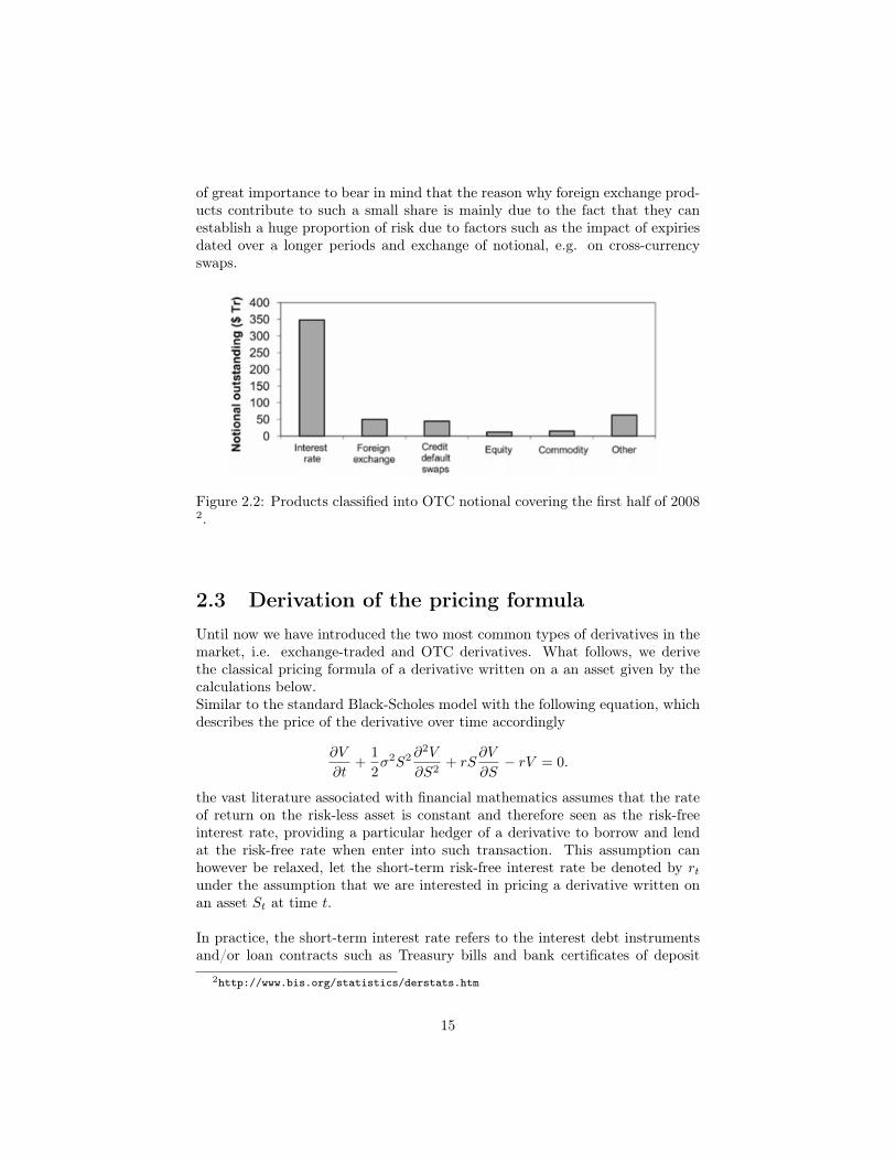
of great importance to bear in mind that the reason why foreign exchange prod-ucts contribute to such a small share is mainly due to the fact that they canestablish a huge proportion of risk due to factors such as the impact of expiriesdated over a longer periods and exchange of notional, e.g. on cross-currencyswaps.

Figure 2.2: Products classified into OTC notional covering the first half of 20082.

2.3 Derivation of the pricing formulaUntil now we have introduced the two most common types of derivatives in themarket, i.e. exchange-traded and OTC derivatives. What follows, we derivethe classical pricing formula of a derivative written on a an asset given by thecalculations below.Similar to the standard Black-Scholes model with the following equation, whichdescribes the price of the derivative over time accordingly

∂V

∂t+

1

2σ2S2 ∂

2V

∂S2+ rS

∂V

∂S− rV = 0.

the vast literature associated with financial mathematics assumes that the rateof return on the risk-less asset is constant and therefore seen as the risk-freeinterest rate, providing a particular hedger of a derivative to borrow and lendat the risk-free rate when enter into such transaction. This assumption canhowever be relaxed, let the short-term risk-free interest rate be denoted by rtunder the assumption that we are interested in pricing a derivative written onan asset St at time t.

In practice, the short-term interest rate refers to the interest debt instrumentsand/or loan contracts such as Treasury bills and bank certificates of deposit

2http://www.bis.org/statistics/derstats.htm

15

having expiries of less than one year.

Moreover, the underlying asset pays continuous dividends δt. Under the physicalmeasure P

dStSt

= µtdt+ σtdWt

where µt is the drift, Wt a Brownian motion and σt the volatility.

In the event of a replication portfolio, the corresponding replication formulafor a derivative Vt reads as,

Vt = αtSt +Bt (2.1)

whereas αt tells us the number of purchased shares of St and Bt represents thevalue deposited in the risk-free bank account.

The price process B is the price of a risk-free asset should it has the follow-ing dynamics.

dBt = rtBtdt

where r is any adapted process. The B-dynamics can be written as,

dBtdt

= rtBt (2.2)

Let Q be a risk-neutral measure equivalent to P and replacing the P-drift termfor St, that is µt, by (rt − δt), which is the Q-drift term for St. Subsequently,applying Ito’s Lemma to equation (2.1)(∂Vt

dt+

1

2σ2tS

2t

∂2Vt∂S2

t

)dt+

∂Vt∂St

dSt = αt(dSt + δtStdt) + (−αtSt + Vt)rtdt (2.3)

In the beginning of this section we claimed that the hedger of a particularderivative is assumed to borrow and lend at risk-free interest rate. Now let αconstitute the hedge of the derivative, therefore in order to hedge the derivativeVt, we set

αt =∂Vt∂St

Consequently, applying the hedging equation to (2.3) we obtain

∂Vt∂t

+ (rt − δt)St∂Vt∂St

+1

2σ2tS

2t

∂2Vt∂S2

t

= rt Vt (2.4)

where rt is the discount rate.

16

Under the assumption that Vt has no cash flows until its expiry T , the solu-tion of equation (2.4) with the terminal condition Vt = g(St), where g is thecorresponding contract function for the derivative, becomes

VtBt

= EQ[ VTBT|Ft]

(2.5)

where Q is the risk-neutral measure equivalent to P such that µQt = rt − δt

under which bothVtBt

andSte

∫ ts=0

δsds

Btare martingales and Ft contains all the

information known at time t.

Thus, we have derived a simple pricing formula for a derivative written onan asset in its simplest case by applying Ito’s lemma to our pricing equationwhich further can be hedged by using αt.

2.4 Derivative TransactionsIn the following section, we try to illustrate the difference between an OTCderivative transaction schedule and the corresponding one for an exchange tradedderivative. The set-up between the two is somewhat different due to the differ-ences for the two derivative classes which we pointed out earlier in this chapter.

17

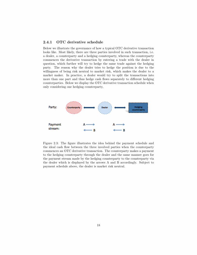
2.4.1 OTC derivative scheduleBelow we illustrate the governance of how a typical OTC derivative transactionlooks like. Most likely, there are three parties involved in such transaction, i.e.a dealer, a counterparty and a hedging counterparty, whereas the counterpartycommences the derivative transaction by entering a trade with the dealer inquestion, which further will try to hedge the same trade against the hedgingparty. The reason why the dealer tries to hedge the position is due to thewillingness of being risk neutral to market risk, which makes the dealer to amarket maker. In practice, a dealer would try to split the transactions intomore than one part and thus hedge cash flows separately to different hedgingcounterparties. Below we display the OTC derivative transaction schedule whenonly considering one hedging counterparty,

Figure 2.3: The figure illustrates the idea behind the payment schedule andthe ideal cash flow between the three involved parties when the counterpartycommences an OTC derivative transaction. The counterparty makes a paymentto the hedging counterparty through the dealer and the same manner goes forthe payment stream made by the hedging counterparty to the counterparty viathe dealer which is displayed by the arrows A and B accordingly. Subject topayment schedule above, the dealer is market risk neutral.

18

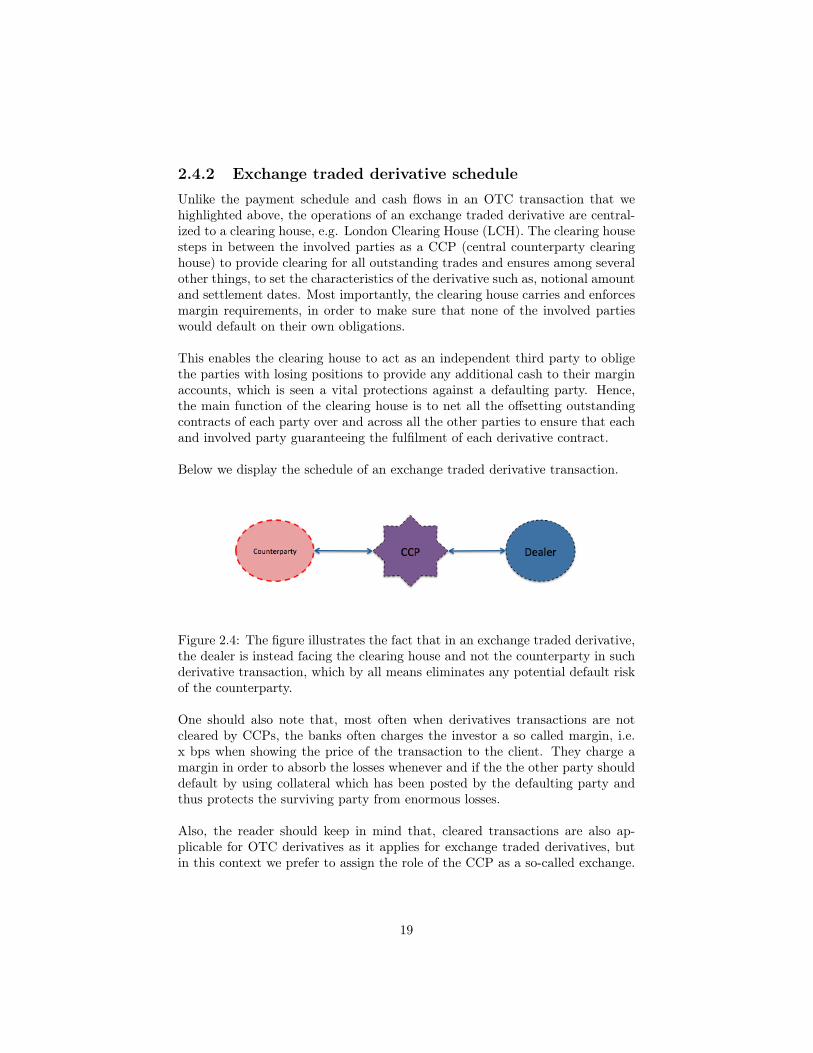
2.4.2 Exchange traded derivative scheduleUnlike the payment schedule and cash flows in an OTC transaction that wehighlighted above, the operations of an exchange traded derivative are central-ized to a clearing house, e.g. London Clearing House (LCH). The clearing housesteps in between the involved parties as a CCP (central counterparty clearinghouse) to provide clearing for all outstanding trades and ensures among severalother things, to set the characteristics of the derivative such as, notional amountand settlement dates. Most importantly, the clearing house carries and enforcesmargin requirements, in order to make sure that none of the involved partieswould default on their own obligations.

This enables the clearing house to act as an independent third party to obligethe parties with losing positions to provide any additional cash to their marginaccounts, which is seen a vital protections against a defaulting party. Hence,the main function of the clearing house is to net all the offsetting outstandingcontracts of each party over and across all the other parties to ensure that eachand involved party guaranteeing the fulfilment of each derivative contract.

Below we display the schedule of an exchange traded derivative transaction.

Figure 2.4: The figure illustrates the fact that in an exchange traded derivative,the dealer is instead facing the clearing house and not the counterparty in suchderivative transaction, which by all means eliminates any potential default riskof the counterparty.

One should also note that, most often when derivatives transactions are notcleared by CCPs, the banks often charges the investor a so called margin, i.e.x bps when showing the price of the transaction to the client. They charge amargin in order to absorb the losses whenever and if the the other party shoulddefault by using collateral which has been posted by the defaulting party andthus protects the surviving party from enormous losses.

Also, the reader should keep in mind that, cleared transactions are also ap-plicable for OTC derivatives as it applies for exchange traded derivatives, butin this context we prefer to assign the role of the CCP as a so-called exchange.

19

Chapter 3

Credit Risk Relationships

This chapter will review some important components of credit risk measure-ment as a foundation of the capital at banks disposal subject to the DVA andFVA. Capital is used to buffer banks against unexpected losses and changes inasset values. Nowadays banks and financial institutions take strategic risk ineveryday operations, these risks are reflected in the volatility of the value ofthe banks assets and therefore presented commonly in finance under differentcircumstances in order to mitigate different types of risk. We start off by intro-ducing two important factors when dealing with OTC derivatives, i.e. Exposureand Loss Given Default (LGD) and finish off by looking at their inclusion in dif-ferent concepts of managing counterparty credit risk under Netting Agreements,ISDA Master Agreement, Collateralization and CSA Collateralization

3.1 Loss Given DefaultLoss Given Default (LGD) describes the percentage of loss when a bank’s coun-terparty goes default and moreover, the amount of funds that are lost by aninvestor when a borrower fails to make his repayments [4]. LGD is a corecomponent of credit risk measures within the vast financial institutions andcorporates, used to determine capital requirements and to assess and managecredit risk, i.e. the expected loss.More specifically, the LGD is in bottom line the estimate of the proportion ofExposure at default (EAD), that will be lost in the event of a defaulting coun-terparty. Furthermore, EAD can in brief be described as the estimated amountthat will be owed by an obligor at the point of such a default. The LGD is givenby,

LGD = 1−R

whereas, the recovery rate, denoted by R, is the ratio of the exposure that wouldbe recovered in an event of default, which has a major role in the concept ofcalculating both the DVA and FVA, since it reflects the amount of losses a firmis exposed to.

20

The recovery rate is calculated as,

R =Net Recoveries

EAD∗ 100%

In order to enhance the methodology of LGD, we illustrate below a simple ex-ample.

At the point of a defaulting counterparty, a bank’s EAD is EUR 5 million,whereas the gross recoveries of EUR 750,000 are made and costs of EUR 75,000are incurred. Therefore, on a non-discounted basis, the recovery rate can becalculated as follows,

R =EUR 750, 000− EUR 75, 000

EUR 5millions∗ 100% = 13, 5%

Hence, the LGD value is,

LGD = 1− 13, 5% = 86, 5%

21

3.2 ExposureThe exposure of a derivative contract represents the amount that would be lostshould a counterparty default.The exposure depends on whether the contractis an asset or a liability to the investor. The very first thing a bank has to do,should the counterparty default, is to close out its positions with that counter-party. Furthermore, to determine the exposure as a consequence of the default,one usually assume that the bank enters into a similar derivative contract witha different counterparty mainly due to maintain its markets position [12]. Insuch a scenario, we can state that, the bank will end up with a net loss of zerosince after entering into a similar contract with another counterparty, they willreceive the market value of the contract and thus the bank ends up with havinga net loss of zero.

On the other hand, should the derivative contract be positive from the banksperspective in the event of default, the bank closes out its position immediately,but this time without receiving anything by the defaulting party. Once again,the bank finds an another party to enter into a similar contract with and hencethe bank pays the market value of the derivative contract and eventually thebank suffers from a net loss equal to the corresponding derivative contract’smarket value.

Subsequently, with respect to the two scenarios above, we can conclude thatthe credit exposure of a bank, which only has one derivative contract with acounterparty, is the maximum of that contract’s market value and zero. Let thevalue of derivative contract i at time t be Vi(t), the contract level exposure isthen given by

Ei(t) = max{Vi(t), 0} (3.1)

We are aware of that the value of the contract may vary unpredictably over timedepending on different market conditions and thus only the current exposure canbe known with a certainty whilst the future exposure is unsettled [12]. As wemention earlier in this section, the contract can either be an asset or a liabilityfrom the banks perspective, which makes the counterparty risk bilateral betweenthe bank and its counterparty in such derivative contract.

3.3 NettingThe word netting itself, refers to a type of a settlement of mutual obligationsbetween two counterparties that processes the combined value of the involvedtransactions. Furthermore, netting has lately been a common practice in tradingof options, foreign exchange and futures. Since netting is exclusively designedto lower the number of transactions required, let us therefore draw an exampleto this notion. For example, if Bank X is owe bank Y e10,000, whilst Bank Yis owe Bank X e2,500, then the value after the netting has taken place wouldbe a e7,500 transfer from bank X to Bank Y.

22

According to [6] netting refers to the fact that single exposures to the overalltransactions are non-additive and hence, the risk tends to be reduced signif-icantly. Subsequently, the overall credit exposure in derivatives markets willgrow at a slower pace in relation to the notional growth of the relevant marketitself.

Netting is considered to be one of the risk mitigation methods, with the greatestimpact on the structure of derivatives markets. In the absence of netting, liquid-ity would dry up and the size of the derivatives market would shrink drastically.The benefit of netting is thus the ability to hedge against underestimating oroverestimating the underlying risk of the overall transactions. However, whennot taking netting into account one can analyze the different transactions out-standing independently with the respective counterparty, as the exposures willstay additive.

The most common types of netting used in the market are:

• Payment netting which covers a situation in which a financial institutionought to make and receive several payments during a given day. This firsttype of netting refers to an agreement to combine the embedded cash flowsinto a single net payment.

• Close-out netting is considered to be more significant to counterparty risk,as it lowers pre-settlement risk. This latter type of netting covers thenetting of the value of a derivative contract in the event of a defaultingcounterparty at a future date.

3.4 Netting AgreementsMost often, should there be several outstanding trades faced towards a default-ing party whilst leaving the exposed risk from the same counterparty unmiti-gated by any means, then one can express the prevailing maximum loss that thebank is exposed to as the sum of the contract-level credit exposures accordingly,

E(t) =∑i

Ei(t) =∑i

max {Vi(t), 0} (3.2)

Furthermore, the exposure that the bank is exposed to in such situation can bemitigated and further reduced by the notion of netting agreements. A nettingagreement is in fact, a legally stipulated document between the two concernedand exposed parties, should one party default, which allows a type of aggregationof the outstanding transactions between the two parties to take place. Moreover,netting enables thus derivative transactions with negative value to be used tooffset the transactions with positive value and thus only the net positive valuedesignates credit exposure at the time of a potential default[12]. Therefore, the

23

total credit exposure arising from all derivative transactions in a netting set(solely those under the jurisdiction of the netting agreement) is reduced to themaximum of the net portfolio value and zero. This total credit exposure is givenby

E(t) = max

{∑i

Vi(t), 0

}(3.3)

Moreover, there could also be several netting agreements with only one coun-terparty.

We sum up this section by looking at the case where there may be trades thatare not covered by any netting agreement at all. Let NAk represent the kth netting agreement with a counterparty. Consequently, we can express thecounterparty-level exposure as,

E(t) =∑k

max

[ ∑i∈NAk

Vi(t), 0

]+

∑i/∈{NA}

max [Vi(t), 0] (3.4)

where the inner sum in the first term sums the values of all trades that is onlycovered by the k th netting agreement, whilst the outer sum, sums up the ex-posures over all netting agreements. The latter term in the equation above issimply the sum of contract-level exposures of all trades that are not covered byany netting agreement [12].

Therefore, we can conclude that the netting agreement allows one to net thevalue of trades with the counterparty that will default before landing the actualclaims and is hence, vital when recognizing the potential benefit of offsettingtrades with a counterparty going into default.

3.5 Trading Relationship under ISDA Master Agree-ment

The International Swaps and Derivatives Association (ISDA) was founded in1985 to ensure that the OTC derivatives markets operate in a safe and effi-cient manner. Moreover, they aim towards reducing the counterparty creditrisk and increasing transparency within the derivatives markets while improv-ing the industry’s operational infrastructure, building robust, stable financialmarkets together with a strong financial regulatory framework.

Published by the ISDA, the Master Agreement has a global scope designedto reduce and eliminate legal uncertainties and to provide tools in order to mit-igate the counterparty risk for parties entering into OTC derivatives.

The Master Agreement contains a qualifying master netting agreement, cor-responding to an agreement between two firms and outlines the contractual

24

obligations and standard terms that will eventually apply to all future out-standing transactions between the firms. Hence, all outstanding transactionsbetween the two parties are handled by one agreement that enables both par-ties to collect the amounts due for each single trade and replace them with anet amount payable to one another. The convenience of a master agreementis mainly because it enables the counterparties to quickly negotiate upcomingfuture agreements or transactions, since both parties can rely on the contractualterms of the master agreement in order to avoid that the same terms will berepetitively negotiated once again and only to consider the deal-specific terms.

3.6 Trading Relationship under Collateralizationand CSA

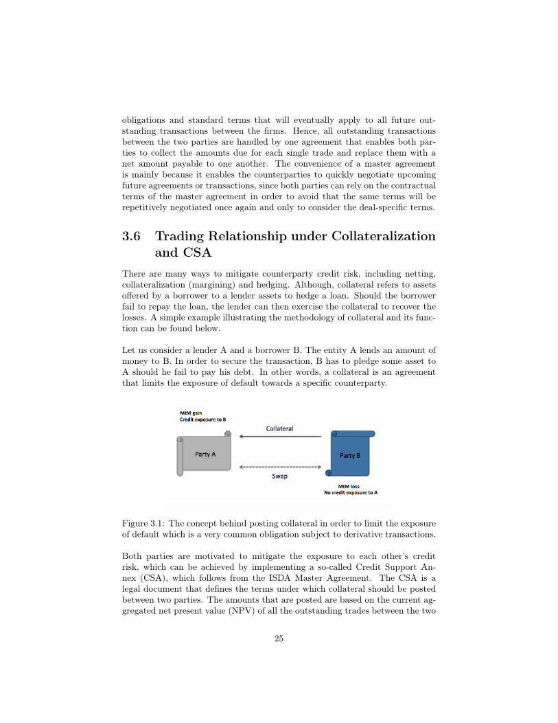
There are many ways to mitigate counterparty credit risk, including netting,collateralization (margining) and hedging. Although, collateral refers to assetsoffered by a borrower to a lender assets to hedge a loan. Should the borrowerfail to repay the loan, the lender can then exercise the collateral to recover thelosses. A simple example illustrating the methodology of collateral and its func-tion can be found below.

Let us consider a lender A and a borrower B. The entity A lends an amount ofmoney to B. In order to secure the transaction, B has to pledge some asset toA should he fail to pay his debt. In other words, a collateral is an agreementthat limits the exposure of default towards a specific counterparty.

Figure 3.1: The concept behind posting collateral in order to limit the exposureof default which is a very common obligation subject to derivative transactions.

Both parties are motivated to mitigate the exposure to each other’s creditrisk, which can be achieved by implementing a so-called Credit Support An-nex (CSA), which follows from the ISDA Master Agreement. The CSA is alegal document that defines the terms under which collateral should be postedbetween two parties. The amounts that are posted are based on the current ag-gregated net present value (NPV) of all the outstanding trades between the two

25

parties. The party that has a negative present value (PV) in the outstandingtrades (also called the Pledgor) is obligated to post collateral CSA. The partythat receive the collateral is normally called the Secured Party [6].

Depending on the direction of the collateral as per the CSA agreement, it mayeither be bilateral or unilateral. The most common for a derivatives contract isa bilateral agreement, meaning that both can receive collateral and are expectedto mitigate the counterparty risk for both parties. This sort of agreement is themost used within the OTC market. On the other hand, in a unilateral agree-ment only one of the parties has the obligation to post collateral to the otherparty.

We have seen different ways of how to mitigate the counterparty credit riskfor OTC derivatives, but at end of the day it can never be completely covered,since there will always be an existing risk in derivative agreements and trans-actions. Below we try to illustrate a common situation in practice, that is anegotiated ISDA Master Agreement between a counterparty and a dealer cou-pled with a negotiated ISDA Master Agreement with CSA between the dealerand the hedging counterparty.

Figure 3.2: The figure shows the current contractual trading relationship men-tioned above, between counterparty, dealer and the hedging counterparty.

26

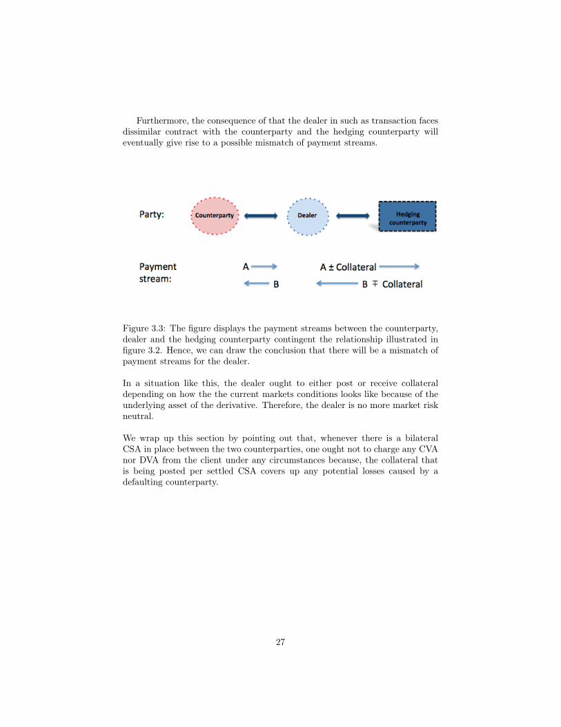
Furthermore, the consequence of that the dealer in such as transaction facesdissimilar contract with the counterparty and the hedging counterparty willeventually give rise to a possible mismatch of payment streams.

Figure 3.3: The figure displays the payment streams between the counterparty,dealer and the hedging counterparty contingent the relationship illustrated infigure 3.2. Hence, we can draw the conclusion that there will be a mismatch ofpayment streams for the dealer.

In a situation like this, the dealer ought to either post or receive collateraldepending on how the the current markets conditions looks like because of theunderlying asset of the derivative. Therefore, the dealer is no more market riskneutral.

We wrap up this section by pointing out that, whenever there is a bilateralCSA in place between the two counterparties, one ought not to charge any CVAnor DVA from the client under any circumstances because, the collateral thatis being posted per settled CSA covers up any potential losses caused by adefaulting counterparty.

27

Chapter 4

Valuation Adjustments

This chapter will present the underlying theory that is used as the basis forour thesis. We will try to provide a comprehensive description for the severalvaluation adjustments that play a major role today and that have to be takeninto account when pricing OTC derivatives. These are the Credit ValuationAdjustment, Debit Valuation Adjustment and Funding Value Adjustment.

4.1 XVAsIn recent years there has been a profusion of adjustments to the risk-neutral priceof an OTC derivative, often denoted as X-Value Adjustments (XVAs). This isthe effect of the new trading environment, which is dominated to a great extentby credit, funding and capital costs. As a reaction to the 2008 financial crisis,financial institutions have become more aware of the adjustments that must beconsidered when valuing derivatives. Most if not all financial institutions haveredeveloped their calculation models of the adjustments in the post-crisis period,having previously taken them for granted. In general, the financial markets havebecome more aware of counterparty credit risk and its importance, which hasgiven rise to several types of valuation adjustments.

4.1.1 CVA − Credit Valuation AdjustmentIn the aftermath of the recent financial crisis, it has become crucial to accountfor the risk of counterparty credit deterioration from the market perspective andfurther the default in pricing of OTC derivative transactions. The pricing com-ponent arising from this risk is the Credit Value Adjustment (CVA). In orderto enable fair pricing when accessing the CCR, the CVA has been evolved tocalculate the future risk for counterparties in the derivatives market. In brief,one can say that CVA is the difference between the risk-free value of a portfolioand the fair value of the same portfolio when taking the possible default of acounterparty into consideration. The CVA is an expected value incorporating

28

both exposure and the probability of default, and aiming towards achieving fairpricing of derivatives.

CVA can be treated as either bilateral or unilateral whereas the latter is givenby the risk-neutral expectation of the discounted loss. In bottom line, CVAis the amount in risk, which is subtracted from the mark-to-market value ofderivative position in order for investors to account for the losses they wouldexpect to suffer from a counterparty default. The discounted loss, L is given by,

L = 1{τ≤T}(1−R)w(t)E(τ)

where τ is a random variable, i.e. a stopping time that denotes the defaultby the counterparty, T is the expiry of the longest transaction in the portfolio,w(t) is the future value of one unit of the base currency invested today at theprevailing interest for expiry t and 1{t≤T} is the indicator function accordingly.

Furthermore, we can define the unilateral (one-way) CVA in terms of risk-neutral expectation as,

CV Auni = EQ [L] =

∫ T

0

(1−R(t))EQ [w(t)E(t)|τ = t] q(t)dt

where q(t) is the probability density function of τ with respect to the probabilitymeasure Q and E(t) is the exposure at time t. Thereto, the middle expressionis equal to the expression with conditional expectation because of mathemat-ical properties of conditional expectations, which stems from the tower property.

Also bear in mind that when expressing the unilateral CVA in terms of condi-tional expectation corresponds conveniently to the fact that the bank will onlysuffer from potential expected losses if and only if, the other party defaults postentering such derivative transaction [12].

The bilateral CVA refers thus to the counterparty credit risk that both par-ties face in an OTC derivative contract, which in turn leads to the CCR of bothcounterparties being affected by an OTC contract. This is mainly due to factthat the OTC market is constructed so that both parties that are committed toa contract will face a credit risk. This will therefore have an effect on the CCRof both counterparties in a bilateral transaction, e.g. two parties entering intoan IRS transaction. Nowadays CVA has become a valuable instrument in thederivatives market, mainly due to the substantial growth of the OTC deriva-tives, whilst the frequency at which CVA is calculated has increased remarkably.It is estimated on a daily basis and occasionally in real-time data [6].

29

4.1.2 DVA − Debit Valuation AdjustmentUntil at the beginning of this century, large banks charged their corporate clientsfor the counterparty credit risk, where the unilateral CVA was taken into ac-count. The CVA was adjusted according to the unilateral counterparty creditrisk, which was constructed on the assumption that the counterparty had acredit risk and the investor as free of default risk. Prior to the financial cri-sis it was set that large banks were not default-charged. This has lately beencriticized and large financial institutions have raised their awareness towardsit. Banks have started to implement CVA between themselves and large cor-porates have also become aware that they face CCR arising from transactionswith banks with a default risk. This has allowed the counterparties to chargeeach other with unilateral CVA, resulting in taking the DVA and bilateral CVAinto account.

Debit Value Adjustment, (DVA) is more or less the opposite of CVA. It re-flects the credit risk that the investor faces towards the other party. It definesthe differences between the value of a derivative/financial-instrument, under theassumption that the bank is default risk-free and the default risk of the bank.When banks have changes in their own credit risk, it can result in changes tothe DVA and also to the bilateral CVA against the counterparty. The DVA issensitive to the bank’s creditworthiness (credit spreads and the probability ofdefault) and changes that affect the expected exposure. The CVA and DVAhave the opposite signs and while CVA decreases the value of a derivative, theDVA increases the value of the same derivative.

If a firm experiences a fall in its credit rating, it will cause an increase onMtM profits for the same firm. This is due to an increase in the probability ofdefault and a depreciation of the credit rating; the firm will therefore have adecrease on the bilateral CVA. Let CV A1

Bilateral and CV A2Bilateral denote the

bilateral CVA before and after the firm faces this decline in credit rating - theformula below represents the bilateral CVA that is calculated as the differencebetween the unilateral CVA towards the counterparty and the DVA [6].

CV A1Bilateral = CV AUnilateral −DV A.

An increase in DVA will have a negative impact on CVA;

CV A2Bilateral = CV AUnilateral − (DV A+ ∆DV A) = CV A1

Bilateral −∆DV A.

Now if we were to apply the reasoning above to the practice of a firm, thenthis would mean that their current outstanding OTC derivative transactionshave become less risky, as well as improving the MtM value of the derivative.Whether this is a realistic or a reasonable outcome is disputed. At this point

30

we can consider that DVA has a major impact when it comes to measuringcounterparty credit risk and it will continue to do so, as the CCR frameworkcontinues to develop. With today’s new regulations it is a requirement of therespective bank to calculate DVA according to the report [6], IFRS 13: FairValue Measurement 1.

1Fair Value Measurement - International Financial Reporting Standards 13, May 2011

31

4.1.3 FVA − Funding Value AdjustmentFunding Value Adjustment (FVA) is, in the existence of an ISDA Master Agree-ment, an adjustment to the value of a derivatives portfolio which is designed toguarantee that the dealer of a contract recovers its average funding costs whenit trades and hedges derivatives. When traders need to manage their tradingpositions, they need to gather cash in order to perform a number of operations(hedging positions and posting collateral). It is obtained from the treasury de-partment or from the money market that has to be satisfied. Traders can alsogather cash from its market position such as coupons, collateral and close-outpayments. This will result to some revenue for the trader in which he is notready to lend it for free and hence FVA goes in both ways, sometimes you gainfrom it and sometimes you lose depending on the circumstances of the trade.

Basically, FVA corresponds to a funding cost/benefit from borrowing or lendingcash arising from day-to-day derivatives business operations, for example whenposting and receiving collateral. Consider a situation where the dealer is to postcash collateral on the hedge, but does not receive that cash in return from theits counterparty. The situation requires thus that the dealer has to raise thecash itself in order to cover the deficit caused by the counterparty.

Subject to the scenario above, many theoretical arguments claim that the dealer’svaluation should recover the total amount of its funding costs, while otherdealers find these arguments unconvincing and therefore make the adjustmentnonetheless. The raised issues involved in the FVA debate (whether productsshould be valued following cost prices or at market prices) are essential to manyindustries beyond the derivative market when thoroughly evaluating potentialinvestments [8].

When taking the credit risk into account, pricing models such as the Black-Scholes-Merton play a crucial role for derivatives traders in the event of no-default value (NDV) of a derivative transaction. The NDV implies that whetherboth sides of a transaction will live up to their obligations, depends on the dis-count rate that is used in question. At the same time, if we assume that therisk-free rate is used, the resulting value is consistent both with theory and withmarket prices in the interdealer market as full collateralization is required.

According to [10], when adjusting for credit risk, the portfolio is given by

Portfolio Value = NDV - CVA + DVA. (4.1)

Furthermore, in order to incorporate the dealer’s average funding costs for un-collateralized transaction, we implement the adjustment of FVA. One has tobear in mind that there is a difference between the NDV obtained when therisk-free rate is used for discounting and the NDV derived on the discountingat the dealer’s cost of funds. When incorporating FVA in equation (3.1), we

32

obtain the following equation

Portfolio Value = NDV - CVA + DVA - FVA. (4.2)

However, one thing to be aware of is that several theoreticians claims that theFVA is not an adjustment for credit risk, since the CVA and the DVA takethis into account and would otherwise imply double counting for the credit risk.The drawback of FVA is that, different market participants often have differentestimates of the fair value, even though they often use identical models with thesame market data.

Now if we consider the equation (3.1) - should the dealer and the counterpartyhave the same funding costs, this would then imply that the dealer’s FVA isequal in magnitude and contrary in sign to the FVA of the counterparty, whichin turn will make them both still agree on the fair value which would not be thecase in the event of different funding costs.

4.1.4 Double Counting of FVA and DVAWe have until now seen that the FVA concerns funding while the DVA treatsa market participant’s own credit risk and thus they concern different perspec-tives of the uncollateralized derivatives market. This section will be based onthe framework which stems from the article [10] on how these two adjustmentsinteract and potentially overlapping one another.

It has been an enormous controversy regarding the relationship between thesetwo valuation adjustments and whether the DVA should be ignored, which hasraised the question of double counting. In order to examine the likelihood ofa credit event to happen and whether the DVA is overflowed in the contextof FVA, we will throughout this section introduce two distinguished types ofcharacteristic functions, which cover the probability structure in the event of acredit event.

Now let DV Ad refer to the value to a bank that arises in the event of defaulton its own derivatives obligations whilst DV Af reflects the value to the bankbut this time in the event of default on its other liabilities, such as short-termdebt, long-term debt, i.e. the DVA arising from the funding that is required forthe derivatives portfolio.

Under the assumption that the whole of the credit spread is the compensa-tion for default risk one can set the DV Af equal to the FVA for a derivativesportfolio. This could be considered as valid since the PV of the expected ex-cess of the bank’s funding for the derivatives portfolio under the risk-free rateis equal to the FVA. This in turn is also equal to the compensation the bankis providing to its lenders should the bank default and thus equivalent to theexpected benefit to the bank in the scenario of defaulting on its own funding.

33

Consequently, FVA and DV Af will cancel out one another. It is also of greatimportance to bear in mind the fact that whenever a derivative needs funding,FVA is accounted as a cost whilst DV Af as a benefit. This applies for the otherway around, so whenever a derivative provides funding the FVA is treated as abenefit and the DVA as a cost accordingly.

This will extend equation (3.2) to

Portfolio Value = NDV − CV A+DV Ad +DV Af − FV A= NDV − CV A+DV Ad.

(4.3)

Here, both FVA and DV Af are additive across transactions whenever transac-tions being entirely uncollateralized. Therefore, the dealer’s FVA and DV Afare independent of other possible transactions entered into by the dealer for aderivative [10].

Now let us instead take the DV Ad under the scope. Equation (3.3) indicatesand validates that it is appropriate to calculate this for a derivatives portfolio,which the dealer has with its counterparty.Consider the case where a dealer has n uncollateralized transactions with anend user. Moreover, we set up the definition for the value to an end user of theith transaction at time t as vj(t), whereas the dealer’s unconditional defaultrate at time is defined as q(t).

In order to describe the likelihood of a default to occur we introduce threekinds of characteristic functions that describe the probability structure of sucha credit event.The survival function S(t) is the probability that a stopping time, τ , occurs firstafter than any point in time, t,

S(t) = P [τ > t] = 1−Q(t)

where Q(t) is the cumulative distribution function (CDF) of τ .

Furthermore, q(x) is the density function of the PD, meaning that Q(x) =∫ x−∞ q(s)ds. Therefore, the density q has the property that

∫∞0q(s)ds = 1, be-

cause τ ≥ 0.

Moreover,q(t) = Q′(t) = −S′(t).

The relationship between q and S can also be described in terms of the haz-ard rate.The hazard rate λ also called the survival analysis, originates from themathematical insurance and actuarial science concept. It expresses the instan-taneous conditional failure rate and can be defined using conditional probability.

λ(t) = lim∆t→0

P [t < τ ≤ t+ ∆t|τ > t]

∆t=q(t)

S(t)

34

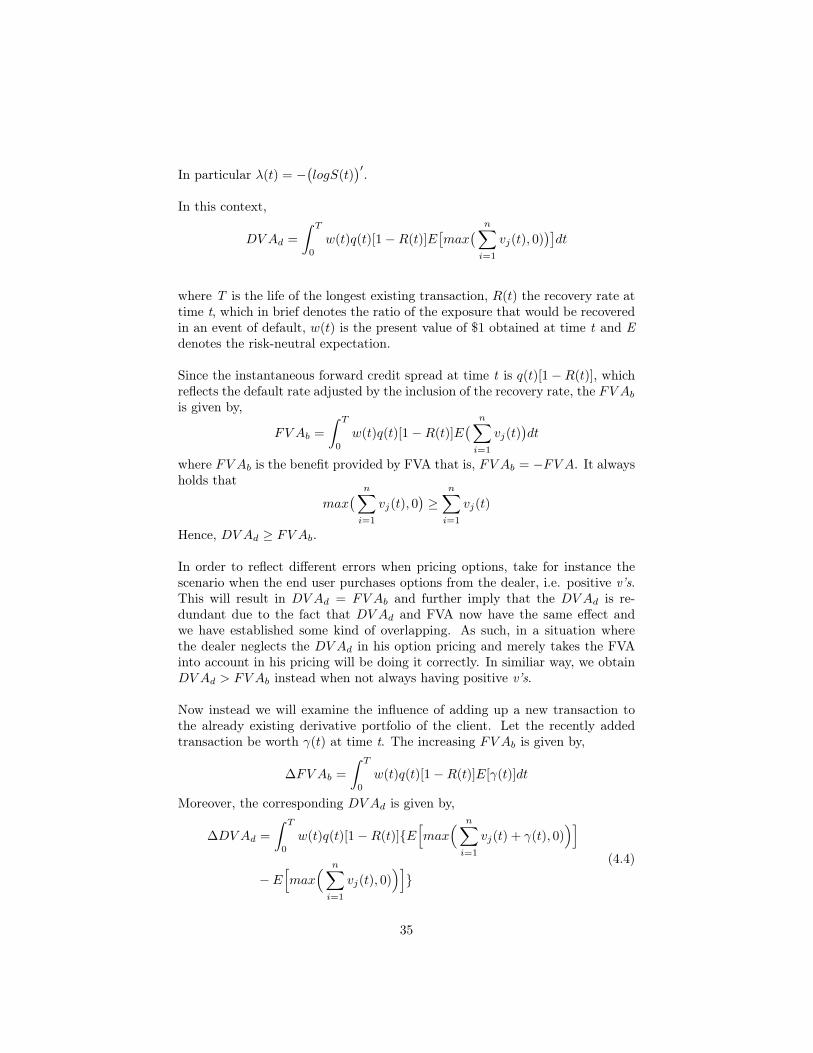
In particular λ(t) = −(logS(t)

)′.In this context,

DV Ad =

∫ T

0

w(t)q(t)[1−R(t)]E[max

( n∑i=1

vj(t), 0))]dt

where T is the life of the longest existing transaction, R(t) the recovery rate attime t, which in brief denotes the ratio of the exposure that would be recoveredin an event of default, w(t) is the present value of $1 obtained at time t and Edenotes the risk-neutral expectation.

Since the instantaneous forward credit spread at time t is q(t)[1−R(t)], whichreflects the default rate adjusted by the inclusion of the recovery rate, the FV Abis given by,

FV Ab =

∫ T

0

w(t)q(t)[1−R(t)]E( n∑i=1

vj(t))dt

where FV Ab is the benefit provided by FVA that is, FV Ab = −FV A. It alwaysholds that

max( n∑i=1

vj(t), 0)≥

n∑i=1

vj(t)

Hence, DV Ad ≥ FV Ab.

In order to reflect different errors when pricing options, take for instance thescenario when the end user purchases options from the dealer, i.e. positive v’s.This will result in DV Ad = FV Ab and further imply that the DV Ad is re-dundant due to the fact that DV Ad and FVA now have the same effect andwe have established some kind of overlapping. As such, in a situation wherethe dealer neglects the DV Ad in his option pricing and merely takes the FVAinto account in his pricing will be doing it correctly. In similiar way, we obtainDV Ad > FV Ab instead when not always having positive v’s.

Now instead we will examine the influence of adding up a new transaction tothe already existing derivative portfolio of the client. Let the recently addedtransaction be worth γ(t) at time t. The increasing FV Ab is given by,

∆FV Ab =

∫ T

0

w(t)q(t)[1−R(t)]E[γ(t)]dt

Moreover, the corresponding DV Ad is given by,

∆DV Ad =

∫ T

0

w(t)q(t)[1−R(t)]{E[max

( n∑i=1

vj(t) + γ(t), 0))]

− E[max

( n∑i=1

vj(t), 0))]}

(4.4)

35

From previous calculations we have shown that the DV Ad ≥ FVA. However∆DV Ad can either be less than or greater than the ∆FV Ab.

The controversy behind this conundrum of including both FVA and DVA inOTC transactions is mainly due to the fact that FVA has the disadvantage ofcreating arbitrage opportunities when prices tend to be favourable since a singleprice cannot serve the purpose of both reflecting the derivative trader’s fundingcosts and still be consistent with the prices regulated by the market. Therefore,in such an optimal scenario for an end user is thus to enter into a transactionwith a bank facing high funding costs and enter into an offsetting transactionwith a bank facing low funding costs in order to avoid both favourable andunfavourable prices when buying and selling options.

36

Chapter 5

DVA on the Balance Sheet

Currently there is a great debate of how to deal with and treat DVA with respectto a bank’s balance sheet. We will further address the accounting perspectiveof DVA, since we believe it adds value and will deepen the understanding ofthis spectrum. This particular section is mostly based on the [5], where theauthors examines the different links and implications subject to Funding, Liq-uidity, Credit and Counterparty Risk. Furthermore, we will go under the scopewith the essence of the DVA coupled with a quite robust conceptual frameworkto consistently encompass the DVA in a balance sheet of a financial institution.It is important to address the tie between DVA and its treatment in banks’balance sheets since derivative contracts have an important impact by valua-tion adjustments on the same balance sheets which will eventually enable us toestablish a thoroughly understanding of the correlation between these, whichstems from the debate over this particular adjustment.

5.1 DVA’s treatment in banks’ balance sheetsRecent researches have provided several but not always satisfying, vindicationsfor the reduction of the liabilities produced by the DVA. In what follows we willtry to highlight and analyze DVA’s incorporation in a balance sheet and if itshould be considered as applicable subject to banks’ balance sheet.

In brief, a balance sheet gives an comprehensive overview of a firm’s assets,liabilities and shareholders’ equities at a prospective time point t. Furthermore,these three segments of a balance sheet gives investors an indication of how muchof the firm assets and liabilities together with the total amount that has beeninvested by the shareholders. Under any circumstances the following formulafor the balance sheet must hold

Assets = Liabilities+ Equities

37

where the two sides should cancel out one another.

Now, let B and L denote two financial institutions as in a regular transaction,whereas the bank B enters into a transaction with bank L in terms of borrow-ing money from the latter one. In this particular case where B = borrower,L=lender, to keep things non-complex, we assume that there is a constant risk-free interest rate r embedded in the transaction between the two parties similarto the one in the Black-Scholes model whereas each single financial institutionpays a funding spread denoted sX , X ∈ {B,L} over the risk-free rate when bor-rowing money. The funding spread is simply the difference between the fundingcosts of a bank and the risk-free rate. The funding spread can be divided intotwo segments:

I) The premium that the lender charges the borrower to cover for the prob-ability of default by the borrower which will be denoted as πX , and the LGDX

(indicated as a portion of the lent amount by the borrower).

II) The liquidity premium when applicable is denoted as γX .

Moreover, we assume that the borrower B is an institution with a balance sheetin its simplest form which is marked to market, corresponding to the fact thatthe accounting for the fair value of their assets or liabilities are based on thecurrent market price. The stockholders determine to commence a transactionactivity with an equity E until time of maturity T, whereas the amount E isdeposited in a bank account BA1 that is assumed to be risk-free. Furthermore,we assume that no premium is required over the risk-free rate, that makes italso to the hurdle rate to value investment projects whilst the borrower doesnot pay any liquidity premium, thus equivalent to sB = πB .

When commencing the transaction at time 0, the bank cuts a deal with a pos-sible lender (institutional investor) to close a loan contract. The bank is notcharging any funding costs when setting the fair amount to lend, and hence thelender does not need to to pay any interest for the funding that they deploy intheir business. The amount is deposited in a bank account BA2, which is alsoassumed to be risk-free.

38

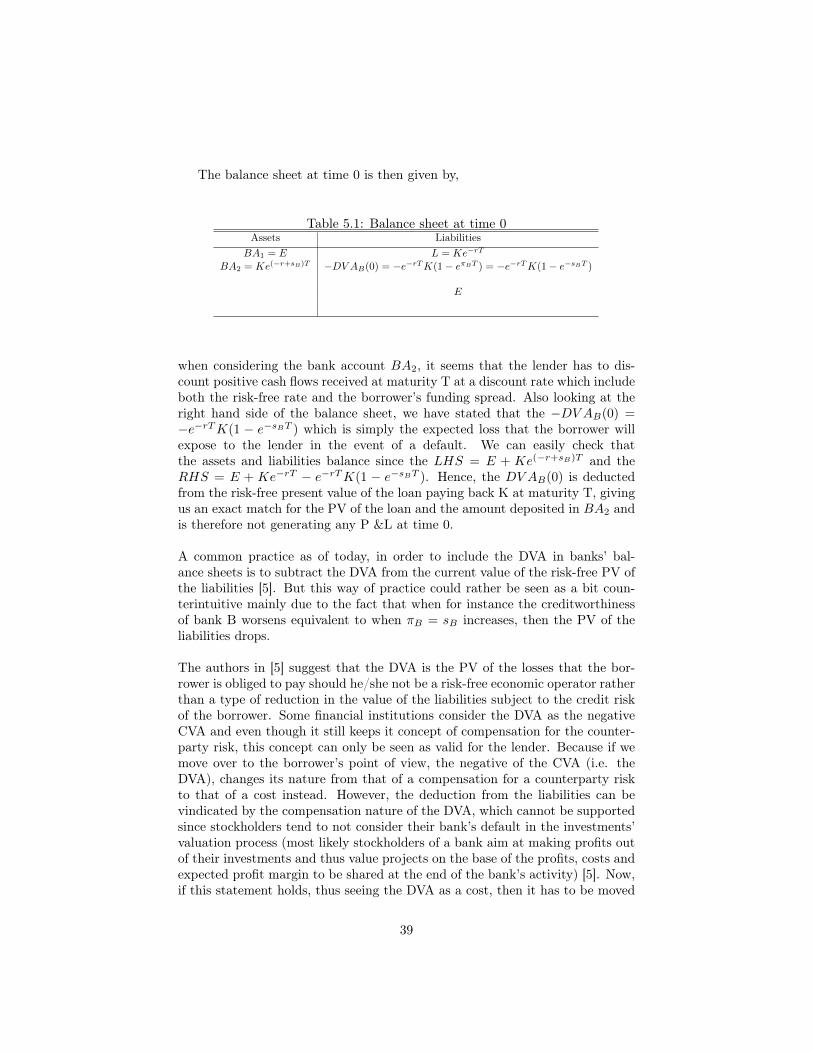
The balance sheet at time 0 is then given by,

Table 5.1: Balance sheet at time 0Assets Liabilities

BA1 = E L = Ke−rT

BA2 = Ke(−r+sB)T −DV AB(0) = −e−rTK(1− eπBT ) = −e−rTK(1− e−sBT )

E

when considering the bank account BA2, it seems that the lender has to dis-count positive cash flows received at maturity T at a discount rate which includeboth the risk-free rate and the borrower’s funding spread. Also looking at theright hand side of the balance sheet, we have stated that the −DV AB(0) =−e−rTK(1 − e−sBT ) which is simply the expected loss that the borrower willexpose to the lender in the event of a default. We can easily check thatthe assets and liabilities balance since the LHS = E + Ke(−r+sB)T and theRHS = E + Ke−rT − e−rTK(1 − e−sBT ). Hence, the DV AB(0) is deductedfrom the risk-free present value of the loan paying back K at maturity T, givingus an exact match for the PV of the loan and the amount deposited in BA2 andis therefore not generating any P &L at time 0.

A common practice as of today, in order to include the DVA in banks’ bal-ance sheets is to subtract the DVA from the current value of the risk-free PV ofthe liabilities [5]. But this way of practice could rather be seen as a bit coun-terintuitive mainly due to the fact that when for instance the creditworthinessof bank B worsens equivalent to when πB = sB increases, then the PV of theliabilities drops.

The authors in [5] suggest that the DVA is the PV of the losses that the bor-rower is obliged to pay should he/she not be a risk-free economic operator ratherthan a type of reduction in the value of the liabilities subject to the credit riskof the borrower. Some financial institutions consider the DVA as the negativeCVA and even though it still keeps it concept of compensation for the counter-party risk, this concept can only be seen as valid for the lender. Because if wemove over to the borrower’s point of view, the negative of the CVA (i.e. theDVA), changes its nature from that of a compensation for a counterparty riskto that of a cost instead. However, the deduction from the liabilities can bevindicated by the compensation nature of the DVA, which cannot be supportedsince stockholders tend to not consider their bank’s default in the investments’valuation process (most likely stockholders of a bank aim at making profits outof their investments and thus value projects on the base of the profits, costs andexpected profit margin to be shared at the end of the bank’s activity) [5]. Now,if this statement holds, thus seeing the DVA as a cost, then it has to be moved

39

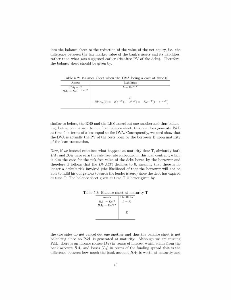
into the balance sheet to the reduction of the value of the net equity, i.e. thedifference between the fair market value of the bank’s assets and its liabilities,rather than what was suggested earlier (risk-free PV of the debt). Therefore,the balance sheet should be given by,

Table 5.2: Balance sheet when the DVA being a cost at time 0Assets Liabilities

BA1 = E L = Ke−rT

BA2 = Ke(−r+sB)T

E−DV AB(0) = −Ke−rT (1− eπBT ) = −Ke−rT (1− e−sBT )

similar to before, the RHS and the LHS cancel out one another and thus balanc-ing, but in comparison to our first balance sheet, this one does generate P&Lat time 0 in terms of a loss equal to the DVA. Consequently, we need show thatthe DVA is actually the PV of the costs born by the borrower B upon maturityof the loan transaction.

Now, if we instead examines what happens at maturity time T, obviously bothBA1 and BA2 have earn the risk-free rate embedded in this loan contract, whichis also the case for the risk-free value of the debt borne by the borrower andtherefore it follows that the DV A(T ) declines to 0, meaning that there is nolonger a default risk involved (the likelihood of that the borrower will not beable to fulfil his obligations towards the lender is zero) since the debt has expiredat time T. The balance sheet given at time T is hence given by,

Table 5.3: Balance sheet at maturity TAssets Liabilities

BA1 = EerT L = KBA2 = KesBT

E

the two sides do not cancel out one another and thus the balance sheet is notbalancing since no P&L is generated at maturity. Although we are missingP&L, there is an income source (P1) in terms of interest which stems from thebank account BA1 and losses (L2) in terms of the funding spread that is thedifference between how much the bank account BA2 is worth at maturity and

40

how much the borrower has paid back on the loan contract which is given by,

(EerT − E) + (KesBT −K) = P1 − L2

if we add these profits and losses to the equity E and further consider the outflowof cash to be paid back on the loan (now we subtract K from BA2 on the LHSinstead of having K = L on the RHS), then the balance is once again balancingand the two sides cancel out each other,

Table 5.4: Balance sheet when outflow of cash is to be paid back on the loanAssets Liabilities

BA1 = EerT L = 0BA2 = KesBT −K

EP1 − L2

hence the debt is equal to zero and the borrower’s loan transaction is uponcompletion at the lender’s disposal. Moreover, if would value its profitability byalso including the hurdle rate then we would obtain,

(EerT − E) + (KesBT −K)− E(erT − 1) = Ke−sBT −K = L2

thus we can conclude that as a whole, this loan contract has generated a loss interms of L2 corresponding to the funding spread for the borrower on the amountK. When examining the last balance sheet it is clear to us that the authors wereright in considering the DVA as the value of the losses suffered at maturity ofthe loan contract rather than as a reduction of the risk-free PV of the loan itself.

First and foremost, we can conclude that whenever the DVA is seen as thePV of a cost, then it simply corresponds to the reduction of the equity E thatcan be agreed upon at the launch of the loan contract which enables the factthat the DVA can be included in a marked to market balance sheet as a reduc-tion of the equity E without any perverse effects should the creditworthinessof the borrower worsens. This is mainly due to the fact that if such scenariowould take place, the PV of the costs would then increase whilst the net equityis diminishing accordingly. Therefore, the DVA should not be neglected into thebalance sheet under any circumstances whatsoever.

Even though we have stipulated the importance of incorporating DVA on thebalance sheet from an accounting point of view, still there are just a few institu-tions that record this particular adjustment. Personally, we believe that thereare a number of reasons for not doing so; the counterintuitive impact of record-ing a gain in P&L as their own creditworthiness becomes progressively worse;

41

entities would most likely not be able to gain an economic benefit from its owncredit gain upon close out of a derivative liability; the likelihood of an increasein the systematic risk that may arise from hedging DVA and most important, itis not mandatory to implement such an adjustment according to the accountingstandards as of yet.

42

Chapter 6

Introduction to Funding Cost

Up to when the credit crisis took place the vast financial institutions borrowedmoney at the LIBOR rate, where the spread primarily between LIBORs withdifferent tenor, i.e. the amount of time left for the repayment of a loan orcontract were quite small. At that time and that environment, the LIBORwas treated as the risk-free rate due to the fact that this was the actual rateat which the most financial institutions too big to fail funded their business.The notation too big to fail stems from the fact that in particular banks are solarge and so interconnected that their failure would be disastrous for the world’seconomy, and they therefore must be supported by government in the event of apotential failure. In the aftermath of the Lehman era, this was no longer valid.It was also noted that the spread between the LIBOR and the overnight rate(OIS) reached levels of approximately 365 basis points in 2008, which could becompared to the 10 basis points before things started to escalate.In order the settle the price of a derivative as of today we need to discount itscorresponding future’s cash flows, the issue still remains though of which risk-free rate we must use for discounting now when we must not use the LIBORrate as the risk-free rate.

6.1 Pricing of the Derivative subject to the fund-ing cost

Here we combine two pricing processes, one for the stock and one for the deriva-tive including their corresponding dynamics. We think of the funding cost as a"negative dividend", which is the difference between the risk-free interest rateand the rate of return. This "negative dividend" can be potentially different forthe derivative we are considering and for the underlying asset, see [10]. Notethat the risk neutral measure is a probability measure such that each share priceis exactly equal to the discounted expectation of the share price under this mea-sure. This is commonly used in the pricing of financial derivatives due to thefundamental theorem of asset pricing, which implies that in a complete market

43

a derivative’s price is the discounted expected value of the future pay-off underthe unique risk-neutral measure.

The risk-free interest rate is the theoretical rate of return of an investmentwith no risk of financial loss. The risk-free rate represents the interest thatan investor would expect from an absolutely risk-free investment over a givenperiod of time. However, a risk-free rate can only be approximated in practicebecause even the safest investments carry a very small amount of risk. Forinstance, the interest rate on a three-month U.S Treasury bill can be used asthe risk-free rate because of its low risk of investment. The risk-free interestrate can also be associated with the LIBOR rate, which is the benchmark forshort-term interest rate that banks charge each other in the London interbankmarket. In a similar way the EURIBOR, Federal Funds Rate or national bondguaranteed by the government in stable economy market would be applicable.

The price process for the stock is defined as dSt and dCS is the negative dividendprocess for the stock. Therefore,

dSt = StµSdt+ StσSdW̄t

dCS = St(r − rs)dt

where µS is the expected return on the stock, σS is the stock’s volatility anddW̄t is a Wiener process [10]. The (r− rs) represent the negative dividend ratefor funding where rs is the funding rate of the stock.

The Derivative written on S with price process π(t) = F (t, S(t)), expiry atT > 0 and pay-off π(T ) = Φ(T ).

The price process for the derivative is defined as dF and dCF is the negativedividend process for the derivative. Therefore,

dF = FµF dt+ FσF dW̄

dCF = F (r − rd)dt

where µF is the expected return on the derivative, σF is the derivative’s volatil-ity. The (r − rd) represent the negative dividend rate for funding where rd isthe funding rate for the derivative.

An example of funding cost could be when a bank search for new capital inorder to reinvest it on other investments (e.g. stocks and derivatives) that cancover the interest rate of holding a debt in the event of issuing a bond. So theinstrument should earn at least the interest rate of the debt rather than the riskfree interest rate, r.

According to [1] we recall the following scheme when determining the arbitragefree price for a T -claim of the form Φ(ST ).

44

• Assume that the pricing function is of the form F (t, St).• Consider µS , σS , Φ, F , rs, rd and r are exogenously given.• Use a self financed portfolio based on the derivative instrument and the

underlying stock.• Form a self-financed portfolio whose value process V has a stochastic dif-

ferential without any driving Wiener process, i.e. it is of the form

dV (t) = V (t)k(t)dt.

• In the absence of arbitrage we must have k = r.• The equation has a unique solution, thus giving us the unique pricing

formula for the derivative, which is consistent with absence of arbitrage.

We combine the processes

dGS = St(µS + r − rs)dt+ σSStdW̄

dGF = F (µF + r − rd)dt+ σFFdW̄

Moreover, we build a portfolio from GS and GF so it is risk-free. Let V (t) bethe value of the portfolio and uS , uF the portfolio coefficients.

dV = V

{uSdGSS

+ uFdGFF

}From Ito’s lemma we have:

µF =1

F

{∂F

∂t+ µSS

∂F

∂s+

1

2σ2SS

2 ∂2F

∂s2

}

σF =1

FσSS

∂F

∂s.

We obtain

dV = V {uS(µS + r − rs) + uF (µF + r − rd)} dt+ {uSσS + uFσF } dW̄

we determine the portfolio weights by excluding the Wiener process in order toeliminate the risk and solve for uS and uF as the solution to the system

uSσ + uFαF = 0,

uS + uF = 1.

The system has the following solution

uS =σF

σF − σS,

uF =−σS

σF − σS,

45

Eventually, if we insert the values for uS , uF , µF and σF into the equation dVwe end up with the following pricing equation:

∂F

∂t+ rsS

∂F

∂s+

1

2σ2S2 ∂

2F

∂s2− rdF = 0,

F (T, s) = Φ(s).

By the Feynman-Kac formula the pricing function of the derivative is given by

F (t, s) = e−rd(T−t)Et,sΦ(XT )

where the dynamics of X are given by

dXt = rsXtdt+ σXtdWt.

X0 = S0

where Wt is a Wiener process.

For instance, see also [10], the funding adjusted price of a European call op-tion for the stock with strike price K and time to to maturity T is given by theformula Π(t) = F (t, S(t)), where

F (t, s) = S0N(BA1)e(rs−rd)T −Ke−rdTN(BA2)

Here N is the cumulative distribution function for the N [0, 1] distribution and

BA1 =ln(S0/K) + (rs + σ2/2)T

σ√T

BA2 = BA1 − σ√T

In a similar way we can derive the price of a European put option on the stockwith strike price K and time to maturity T accordingly

F (t, s) = Ke−rdTN(−BA2)− S0N(−BA1)e(rs−rd)T

46

6.2 Pricing of non-collateralized derivativesThe existence of FVA, is as we have seen, highly correlated to the recent fi-nancial crisis. Prior to the crisis, the bulge bracket banks used to disregardcollateral and funding costs mostly since the funding for posting collateral cantypically be tangible through a combination of low cost funding options but alsodue to this low cost was in beforehand offset by the interest rate (LIBOR) paidon collateral by the receiving party.In the aftermath of the crisis, we cannot hide the fact that it has had an enor-mous impact in the role of funding in the derivatives markets as the fundingbecame costly, and the interest rate paid on collateral no longer offsets the in-creasing cost [8]. The arising risk of credit lines being pulled is also impendingas soon as the firm is perceived to going bankrupt. Therefore, the importance ofvalue funding needs have become a vital part of the risk management strategyof financial institutions.

In this section we will treat the mechanism of pricing non-collateral derivativeswith a different approach as in [6]. Let Vt denote the price of the derivativewritten on an underlying asset St, which pays continuous dividend yield δt.The dynamics of the underlying asset under the physical measure is given by

dStSt

= µtdt+ σtdWt (6.1)

Moreover, in order to price a non collateralized derivative we have to introducesome assumptions.

• Ht := H(t, St) : Derivative written on the underlying asset St in accor-dance to avoid and to hedge against any substantial price movements ofthe derivative Vt subject to its underlying.

• ft : The rate that corresponds to whenever one is in need of capital andyou borrow money in the market which comes with an additional interestrate.

• it : When borrowers need to borrow money in the market, you can chargethem a rate at which you can lend it to them.

• ct : Counterparties in a non-collateralized transaction most likely postcollateral to one another, this rate is equivalent to the rate of the collateralpaid on the posted collateral in such derivative transaction.

• rt : Often one uses repo agreements for funding stocks, i.e. a party sells agovernment security to an investor usually on an overnight basis and paysthem back in the future, which entitles him to an additional interest overand above the value of the securities. This repo rate is designated for theunderlying stock St.

47

Moreover, let us set our sights on the road map for the cash flows that wouldoccur when considering an infinitesimal time interval, seen over t and t+ dt inthe event of funding and hedging any derivative.We provide such an overview in order to highlight the life-cycle of a non-collateralized derivative transaction strategy.

• From the Investor’s point of view, at time t, this is where the actual deriva-tive transaction takes place with three different parties entitled to differentroles. First of there is a Hedger, who ought to enter into a derivative con-tract in the market, priced at Vt. On the side of the transaction we havean Investor which is willing the undertake this derivative at his disposal.Furthermore, depending on the outcome of the price of the derivative Vt,the Hedger will either fund the derivative should Vt > 0 or invest if Vt < 0applicable which is quite logical to see since if the derivative face a pos-itive value, it is in need of funding. Behind the scene of the transactionthere is an interbank who is entitled as the Funding Counterparty. This isdue since the Hedger wants to be risk-neutral in such transaction whereasthe Interbank posses the inherent risk to the expense of obtaining postedcollateral from the Hedger.

At maturity, the Investor will eventually pay back on the loan plus someadditional interest arising, reflecting the time when entered into the trans-action until it hits maturity. Subsequently, when thinking of it, in practicethis could cause some arbitrage opportunities which is in line with the ar-guments of Hull & White [10]. This is a fact since the Hedger in questionwill be entitled to pay an amount corresponding to the rate at which heborrowed money ft in a relative low rate from the bank’s treasury deskwhen in need of posting collateral and earn it for the money at which helent for the same cause.

In practice, the arising cost will most likely passed along to the traders onthe FVA desk, who reimburse it from investors through FVA. Therefore,the process of passing FVA on to investors will be acceptable as long asthe bank’s funding cost remains at a relative low rate in comparison toothers.

• As follows the Hedger will at time t either pay or receive the price atwhich the derivative is priced depending on the outcome of its value andfurther receive the value of the derivative at time upon the maturity datecorresponding to t+ dt.

• It is optimal for the Hedger when entering such a derivative transactionto hedge against variations in the price of the derivative Vt, e.g. to avoidending up with a worthless derivative or an outcome which the Hedger isdisadvantaged by as the underlying stock St giving rise to some unexpectedfluctuations, as such the Hedger agrees to enter into a cash-collateralizedderivative denoted by Ht with corresponding notional amount αt. This

48

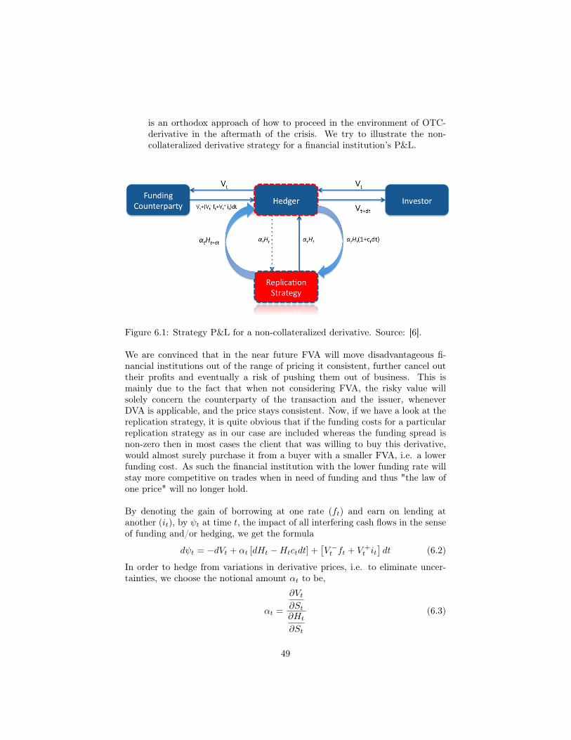
is an orthodox approach of how to proceed in the environment of OTC-derivative in the aftermath of the crisis. We try to illustrate the non-collateralized derivative strategy for a financial institution’s P&L.

Figure 6.1: Strategy P&L for a non-collateralized derivative. Source: [6].

We are convinced that in the near future FVA will move disadvantageous fi-nancial institutions out of the range of pricing it consistent, further cancel outtheir profits and eventually a risk of pushing them out of business. This ismainly due to the fact that when not considering FVA, the risky value willsolely concern the counterparty of the transaction and the issuer, wheneverDVA is applicable, and the price stays consistent. Now, if we have a look at thereplication strategy, it is quite obvious that if the funding costs for a particularreplication strategy as in our case are included whereas the funding spread isnon-zero then in most cases the client that was willing to buy this derivative,would almost surely purchase it from a buyer with a smaller FVA, i.e. a lowerfunding cost. As such the financial institution with the lower funding rate willstay more competitive on trades when in need of funding and thus "the law ofone price" will no longer hold.

By denoting the gain of borrowing at one rate (ft) and earn on lending atanother (it), by ψt at time t, the impact of all interfering cash flows in the senseof funding and/or hedging, we get the formula

dψt = −dVt + αt [dHt −Htctdt] +[V −t ft + V +

t it]dt (6.2)

In order to hedge from variations in derivative prices, i.e. to eliminate uncer-tainties, we choose the notional amount αt to be,

αt =

∂Vt∂St∂Ht

∂St

(6.3)

49

furthermore, by applying Ito to both Vt and Ht in equation (6.2) we obtain thefollowing dynamics

dVt =∂Vt∂t

dt+∂Vt∂St

dSt +1

2

∂2Vt∂S2

t

σ2tS

2t dt

dHt =∂Ht

∂tdt+

∂Ht

∂StdSt +

1

2

∂2Ht

∂S2t

σ2tS

2t dt

(6.4)

which yields

∂Vt∂t

+1

2

∂2Vt∂S2

t

σ2tS

2t − αt

[∂Ht

∂t+

1

2

∂2Ht

∂S2t

σ2tS

2t −Htct

]= V −t ft + V +

t it (6.5)

where[∂Ht

∂t+

1

2

∂2Ht

∂S2t

σ2tS

2t −Htct

]= −(rt − δt)St

∂Ht

∂Stand therefore equation (6.5) reads as,

∂Vt∂t

+ (rt − δt)St∂Vt∂St

+1

2

∂2Vt∂S2

t

σ2tS

2t = V −t ft + V +

t it (6.6)

Moreover, let the spreads over which the Hedger is posting collateral to theFunding Counterparty denote the funding spreads

sft = ft − ct, sit = it − ct

We can thus express equation (6.6) as,

∂Vt∂t

+ (rt − δt)St∂Vt∂St

+1

2

∂2Vt∂S2

t

σ2tS

2t = ctVt + V −t s

ft + V +

t sit

s.t V (T ) = ψ

(6.7)

We have thus found a way of expressing the price of derivative Vt by theFeynman-Kac given by

Vt = EQt

[e−

∫ TtcsdsψT

]−∫ T

t

EQt

[e∫ utcsdssfuV

−u

]du

−∫ T

t

EQt

[e∫ utcsdssiuV

+u

]du

(6.8)

50

Hence,

• Perfect Collateral Price = EQt

[e−

∫ TtcsdsψT

]• Funding Cost =

∫ TtEQt

[e∫ utcsdssfuV

−u

]du

• Funding Benefit =∫ TtEQt

[e∫ utcsdssiuV

+u

]du

where once again, Q is the risk-neutral measure under which cash-collateralizeddeals grow at the pace of the collateral rate while St grows at the repo rate.The perfect collateral price can be defined as the price given by collateralizationin continuous time, with continuous mark-to-market of the investor’s portfolioshould there be any events of default coupled with collateral account inclusiveof margining fees/costs at any time during the lifetime of such derivative trans-action.

We are now ready to make the following statements about FVA and Fund-ing Cost:

We have throughout this section addressed the importance of incorporatingFVA, but on the other hand what is then the opportunity cost of not consid-ering FVA? It is now clear to us that funding cost cannot be ignored shoulda trade have positive P&L coupled with a high potential exposure since, if wewould face disadvantageous market moves on the trade, which will put us outof the money, an enormous funding will be required forthwith to post collateralto the counterparty when in a situation where CSA is present.

The FVA can either be seen as a benefit or a cost from the firm’s point ofview which arises from the fact that the same firm needs to raise money inorder to fund a derivative until maturity.Consequently, the cost arising by the need of funding will be considered as a ben-efit should the derivative generate positive cash flows which enables the Hedgerto reduce our funding needs.

When pricing non-collateralized derivatives correctly, the Hedger of the transac-tion has to, without any loss of generality, discount the derivatives at his fundingrate under the assumption that we are in the environment of having the sameinvestment and funding rate.

We can hereby conclude that the FVA plays a major and a vital role in providingmonetary incentive for the XVA desks to use less funding. This in turn can betangible for instance by charging a higher rate in the event of borrowing fromthe treasury and afterwards paying for the posting money back to where thefunding is originated initially, i.e. to the funding desk. This is why we think theFVA appears in most cases, represented by the sum of both the FCA (fundingcost) and the FBA (funding benefit).

51

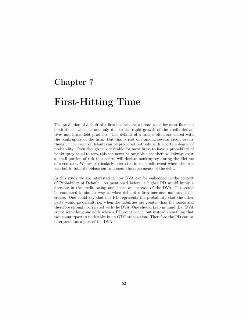
Chapter 7

First-Hitting Time

The prediction of default of a firm has become a broad topic for most financialinstitutions, which is not only due to the rapid growth of the credit deriva-tives and firms debt products. The default of a firm is often associated withthe bankruptcy of the firm. But this is just one among several credit eventsthough. The event of default can be predicted but only with a certain degree ofprobability. Even though it is desirable for most firms to have a probability ofbankruptcy equal to zero, this can never be tangible since there will always exista small portion of risk that a firm will declare bankruptcy during the lifetimeof a contract. We are particularly interested in the credit event where the firmwill fail to fulfil its obligation to honour the repayments of the debt.

In this study we are interested in how DVA can be embedded in the contextof Probability of Default. As mentioned before, a higher PD would imply adecrease in the credit rating and hence an increase of the DVA. This couldbe compared in similar way to when debt of a firm increases and assets de-crease. One could say that our PD represents the probability that the otherparty would go default, i.e. when the liabilities are greater than the assets andtherefore strongly correlated with the DVA. One should keep in mind that DVAis not something one adds when a PD event occur, but instead something thattwo counterparties undertake in an OTC transaction. Therefore the PD can beinterpreted as a part of the DVA.

52

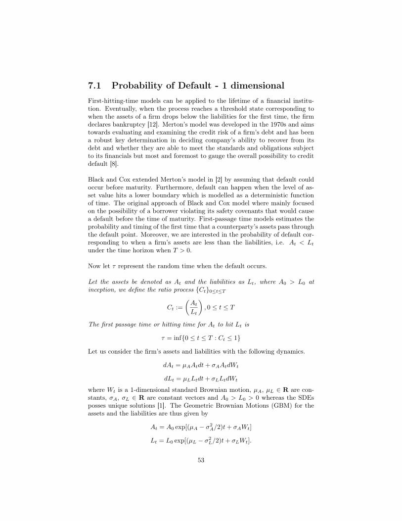
7.1 Probability of Default - 1 dimensionalFirst-hitting-time models can be applied to the lifetime of a financial institu-tion. Eventually, when the process reaches a threshold state corresponding towhen the assets of a firm drops below the liabilities for the first time, the firmdeclares bankruptcy [12]. Merton’s model was developed in the 1970s and aimstowards evaluating and examining the credit risk of a firm’s debt and has beena robust key determination in deciding company’s ability to recover from itsdebt and whether they are able to meet the standards and obligations subjectto its financials but most and foremost to gauge the overall possibility to creditdefault [8].

Black and Cox extended Merton’s model in [2] by assuming that default couldoccur before maturity. Furthermore, default can happen when the level of as-set value hits a lower boundary which is modelled as a deterministic functionof time. The original approach of Black and Cox model where mainly focusedon the possibility of a borrower violating its safety covenants that would causea default before the time of maturity. First-passage time models estimates theprobability and timing of the first time that a counterparty’s assets pass throughthe default point. Moreover, we are interested in the probability of default cor-responding to when a firm’s assets are less than the liabilities, i.e. At < Ltunder the time horizon when T > 0.

Now let τ represent the random time when the default occurs.

Let the assets be denoted as At and the liabilities as Lt, where A0 > L0 atinception, we define the ratio process {Ct}0≤t≤T

Ct :=

(AtLt

), 0 ≤ t ≤ T

The first passage time or hitting time for At to hit Lt is

τ = inf{0 ≤ t ≤ T : Ct ≤ 1}

Let us consider the firm’s assets and liabilities with the following dynamics.

dAt = µAAtdt+ σAAtdWt

dLt = µLLtdt+ σLLtdWt

where Wt is a 1-dimensional standard Brownian motion, µA, µL ∈ R are con-stants, σA, σL ∈ R are constant vectors and A0 > L0 > 0 whereas the SDEsposses unique solutions [1]. The Geometric Brownian Motions (GBM) for theassets and the liabilities are thus given by

At = A0 exp[(µA − σ2A/2)t+ σAWt]

Lt = L0 exp[(µL − σ2L/2)t+ σLWt].

53

Now if we consider the ratioCt =

AtLt

we are proving that division of one GBM by another GBM gives again a GBMaccordingly

=⇒ Ct =A0

L0exp

[(µA − µL −

σ2A

2+σ2L

2

)t+ (σA − σL)Wt

]It is now possible to find a drift coefficient µC and a volatility coefficient σCcompatible with the equation of a GBM.

We want to obtain the following GBM

Ct = C0 exp[(µC −σ2C

2)t+ σCWt]

with σC we do not really have a choice - it has to be σC = σA − σL.Subsequently, this in turn yield the following formulas

µA − µL −σ2A

2− σ2

L

2= µC −

σ2C

2

µA − µL −σ2A

2+σ2L

2= µC −

1

2

(σ2A − σ2

L

)2whereas, the right hand side of the equation describes what we would like µCto solve, and hence leads to a viable formula for µC .

µC = µA − µL + σ2L − σAσB

where the dynamic is given by

dCt = µCCtdt+ σCCtdW.

Furthermore, in order to get the first hitting time τ when At ≤ Lt one cansimulate the probability density function numerically, more precisely we useMonte-Carlo simulation to find the probability density function (PDF) of τ .Theidea is to simulate the dynamics of our Assets and Liabilities and find thefirst time when Ct < 1 and simulate this N = 5000 times. Moreover, we plot ahistogram which will reflect a sort of a density function for the first hitting time.This coupled with a function called allfitdist downloaded from Mathworks1 findsa pretty good fit of the density given some data.

1http://www.mathworks.com/matlabcentral/fileexchange/34943-fit-all-valid-parametric-probability-distributions-to-data/content/allfitdist.m

54

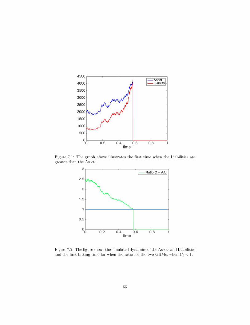
Figure 7.1: The graph above illustrates the first time when the Liabilities aregreater than the Assets.

Figure 7.2: The figure shows the simulated dynamics of the Assets and Liabilitiesand the first hitting time for when the ratio for the two GBMs, when Ct < 1.

55

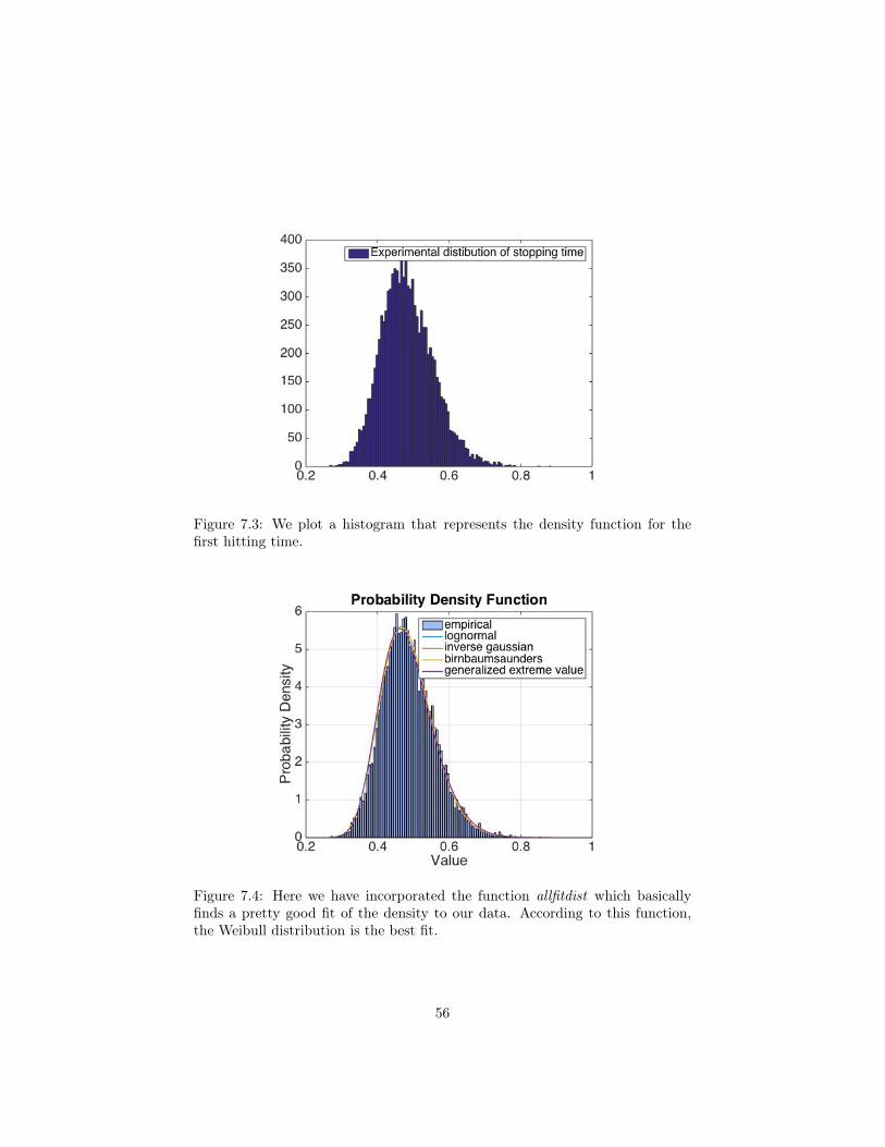
Figure 7.3: We plot a histogram that represents the density function for thefirst hitting time.

Figure 7.4: Here we have incorporated the function allfitdist which basicallyfinds a pretty good fit of the density to our data. According to this function,the Weibull distribution is the best fit.

56

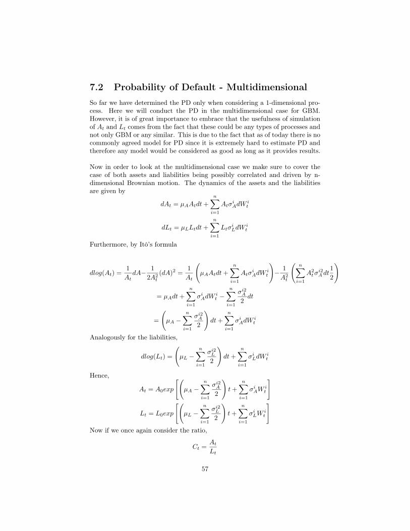
7.2 Probability of Default - MultidimensionalSo far we have determined the PD only when considering a 1-dimensional pro-cess. Here we will conduct the PD in the multidimensional case for GBM.However, it is of great importance to embrace that the usefulness of simulationof At and Lt comes from the fact that these could be any types of processes andnot only GBM or any similar. This is due to the fact that as of today there is nocommonly agreed model for PD since it is extremely hard to estimate PD andtherefore any model would be considered as good as long as it provides results.

Now in order to look at the multidimensional case we make sure to cover thecase of both assets and liabilities being possibly correlated and driven by n-dimensional Brownian motion. The dynamics of the assets and the liabilitiesare given by

dAt = µAAtdt+

n∑i=1

AtσiAdW

it

dLt = µLLtdt+

n∑i=1

LtσiLdW

it

Furthermore, by Itô’s formula

dlog(At) =1

AtdA− 1

2A2t

(dA)2 =1

At

(µAAtdt+

n∑i=1

AtσiAdW

it

)− 1

A2t

(n∑i=1

A2tσi2A dt

1

2

)

= µAdt+

n∑i=1

σiAdWit −

n∑i=1

σi2A2dt

=

(µA −

n∑i=1

σi2A2

)dt+

n∑i=1

σiAdWit

Analogously for the liabilities,

dlog(Lt) =

(µL −

n∑i=1

σi2L2

)dt+

n∑i=1

σiLdWit

Hence,

At = A0exp

[(µA −

n∑i=1

σi2A2

)t+

n∑i=1

σiAWit

]

Lt = L0exp

[(µL −

n∑i=1

σi2L2

)t+

n∑i=1

σiLWit

]Now if we once again consider the ratio,

Ct =AtLt

57

we are proving that division of one GBM by another GBM gives again a GBMbut this time when both assets and liabilities being possibly correlated anddriven by n-dimensional Brownian motion

=⇒ Ct =A0

L0exp

[(µA − µL −

n∑i=1

σi2A2

+

n∑i=1

σi2L2

)t+

n∑i=1

(σiA − σiL

)W it

]

which follows from the fact that,

Cov

(n∑i=1

σiAdWit ,

n∑i=1

σiLdWit

)

=

n∑i=1

σiAσiLdt, σ

iA, σ

iL > 0

On the next page we simulate the stopping for the corresponding process thatwe just derived above.

58

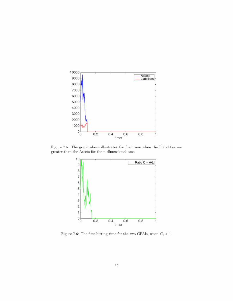
Figure 7.5: The graph above illustrates the first time when the Liabilities aregreater than the Assets for the n-dimensional case.

Figure 7.6: The first hitting time for the two GBMs, when Ct < 1.

59

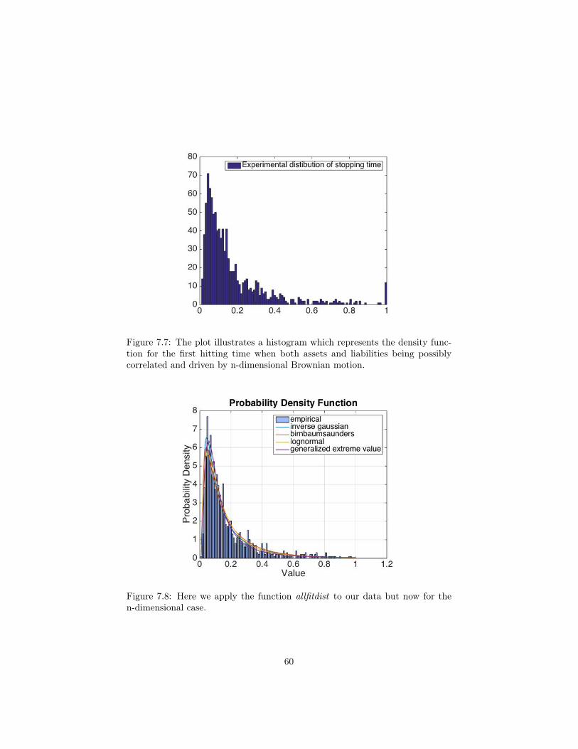
Figure 7.7: The plot illustrates a histogram which represents the density func-tion for the first hitting time when both assets and liabilities being possiblycorrelated and driven by n-dimensional Brownian motion.

Figure 7.8: Here we apply the function allfitdist to our data but now for then-dimensional case.

60

Chapter 8

Funding Strategies for XVAs

In this chapter we will derive a slightly different pricing technique for DVA andFVA from what we have seen earlier in this paper. We address this additonallayer of complexity to pricing derivatives with respect to DVA and FVA bydescribing the authors Christoph Burgard and Mats Kjaer’s approach based onthe article [3]. We will look at funding strategies in terms of when an issuer eitherholds or issues his own bonds. Such a strategy enables the issuer to hedge out agreat share of its cash flows upon the issuer’s default. It is however importantto bear in mind that, the value of derivative instruments does not solely dependon who is funding them, but how they are funded since the funding costs mayfor some reason result in shortfalls or windfalls to bond issuer should their firmgo bankrupt and hence the derived adjustment such as DVA and FVA resultingfrom this depend on the funding strategy employed.

8.1 Set-up prior to semi-replication and pricingLet us consider a simple derivative contract, with collateral possibly beingposted, between an issuer B and a counterparty C. Furthermore, we denotethe value of the derivative as V̂ , which covers the probability of default of boththe issuer and the counterparty coupled with any net funding costs that theissuer may run up against prior to his default. The use of a semi-replicationstrategy is as mentioned above, intended to enable the issuer B to deploy astrategy in order to hedge out market dependent factors and counterparty riskin terms of default which may not always provide an adequate hedge in theevent of B’s own default. In this strategy we use a counterparty zero-couponzero-recovery bond PC , i.e. no coupon payments are made except the repaidface value at the time of maturity whereas no amount will be recovered shouldthe counterparty go bankrupt. Also we have the issuer’s two own bonds de-noted P1 and P2 of different seniors with different recoveries R1 and R2, and Sin order to hedge out the market factor of the underlying derivative contracts,e.g. an asset. The reader should note that, the description of a bond as "senior"

61

does not by itself mean that it is in any way secured and thus investors shouldnot draw any conclusions as to the ranking of a bond solely on the basis ofits description as "senior". The majority of bonds that are issued are seniorunsecured obligations of the issuer.

Moreover, the dynamics for such instruments are given by,

dS = µSdt+ σSdW (8.1)

dPC = rCP−C dt− P

−C dJC (8.2)

dPi = riP−i dt− (1−Ri)P−i dJB (8.3)

where JB and JC indicate the default for the issuer and the counterparty, re-spectively, and P−i/C = Pi/C(t) represent the bond prices prior to any possibledefault. Furthermore, let P1 designate the bond with the lower recovery rate,i.e. R1 < R2 and consequently r1 > r2. If we would end up in a case of zerobasis points between bonds of different seniors it might be trivial to show that,

ri − r = (1−Ri)λB , (8.4)

where r is the risk-free rate of such as case and λB represents the spread of apotentially zero-recovery zero-coupon bond of the issuer [3].

Moreover, let V̂ (t, S, JB , JC) denote the total value of the derivative instrumentfrom the issuer’s point of view, whereas when considering general boundaryconditions upon default of the counterparty or the issuer are given by,

V̂ (t, S, 1, 0) = gB(MB , X) should B default first,

V̂ (t, S, 0, 1) = gC(MC , X) should C default first,

where MB and MC are the amounts equivalent to when unwinding a transac-tions, i.e. resulting in close-out amounts and X represents the collateral postedbetween the parties. In [3] they like to refer these boundaries as "regular",if MB = MC = V , where V is simply the price of the derivative when usingthe classical Black-Scholes formula, i.e. neglecting factors such as any involvedcounterparty, the likelihood of own default and funding costs. For instance, theregular bilateral boundary conditions with collateral are defined as,

gB = (V −X)+ +RB(V −X)−+XgC = RC(V −X)+ + (V −X)−+X. (8.5)

8.2 Semi-replication and pricingIn order to conduct a semi-replication strategy we set up the following hedgingportfolio Π,

Π = δ(t)S(t)+α1(t)P1(t)+α2(t)P2(t)+αC(t)PC(t)+βS(t)+βC(t)−X(t), (8.6)

62

with δ(t) units of S, α1(t), α2(t) and αC(t) represent the own and counterpartybonds, respectively, cash accounts βS(t) and βC(t) and the collateral accountX(t). The cash accounts βS and βC are used to fund S and PC , thereforeαCPC + βC = 0 and δS + βS = 0, which assumed to pay net rates of (qS − γS)and (qC − γC), where q is the funding rate and γ is any potential dividendincome [3]. Since the hedging position can either be collaterlized or repo-ed,qS and qC may also be seen as collateral or repo-rates. Once again X is thecollateral posted subject such a derivative transaction, which further pay therate rX . Consequently, whenever X is positive, the counterparty has posted theamount X in collateral to the issuer.

We would like to design the semi-replication strategy in such way that V̂ +Π = 0.Moreover, the issuer’s bond positions, which we here denote as α1P1 and α2P2

are used to fund and/or invest the outstanding cash that is not funded via thecollateral, which gives us the following funding constraint,

V̂ −X + α1P1 + α2P2 = 0 (8.7)

By combining the funding constraint above with the use of Ito’s lemma, thedefined boundary conditions and the hedging ratios δ and αC , chosen in suchproper way that the risks subject to the market and the default of the counter-party are hedged out, we can express the evolution of the total portfolio overdt. We derive the above steps as follows.

Recall the hedging portfolio we set up earlier, i.e. equation (8.6) whereas thistime we set up the dynamic of the same hedging portfolio which is given by,

dΠ̄ = δ(t)dS(t)+α1(t)dP1(t)+α2(t)dP2(t)+αC(t)dPC(t)+dβ̄S(t)+dβ̄C(t)−dX(t),(8.8)

where dS, dP1, dP2, and dPC are given in equations (8.1) to (8.3) and dβ̄S(t),dβ̄C(t) and dX(t) are the changes in the cash and collateral accounts, βS,C andX when neglecting any potential re-balancing of the two.

Moreover, we draw the assumption that the hedge account βS is collateral-ized, with a funding rate designated by qS coupled with a dividend yield γS . Inaccordance with this, the position for the bond which is held by the counterpartyis assumed to be set up through a repo transaction that costs the counterpartya repo rate of qC . The derivatives collateral account is assumed to cost a col-lateral rate rX [3].

Now by excluding any potential re-balancing of these we would end up withthe following increments in our cash and collateral accounts,

dβ̄S = δ(γS − qS)Sdt, (8.9)

dβ̄C = −αCqCPCdt, (8.10)

63

dX̄ = −rXXdt. (8.11)

The default value of the issuer bond position pre- and post any credit event as-sociated with default is given by, P ≡ α1P1 +α2P2 and PD ≡ R̃1α1P1 +R̃2α2P2.Furthermore, if we insert the equations (8.1) to (8.3) and the increments in ourcash and collateral accounts, i.e. equations (8.9) to (8.11) into the dynamic ofthe hedging portfolio Π (8.8) we obtain the following portfolio,

dΠ̄ = (r1α1P1 + r2α2P2 + λCαCPC + (γ − q)δS − rXX)dt

+ (PD − P )dJB − αCPCdJC + δdS,(8.12)

where λC ≡ rC − qC designates by the spread of the yield of the zero-couponbond PC over its corresponding repo rate and thus is the rate which the coun-terparty hedging position is financed by upon default.

On the other hand, the way dV̂ of the derivative value evolve through its lifetimecan be given by Ito’s lemma for jump diffusions as,

dV̂ = ∂tV̂ dt+ ∂S V̂ dS +1

2σ2S2∂2

S V̂ dt+ ∆V̂BdJB + ∆V̂CdJC , (8.13)

where∆V̂B = V̂ (t, S, 1, 0)− V̂ (t, S, 0, 0) = gB − V̂ (8.14)

∆V̂C = V̂ (t, S, 0, 1)− V̂ (t, S, 0, 0) = gC − V̂ . (8.15)

Moreover, if we combine the way the derivative portfolio evolve in equation(8.13) with the hedging portfolio in equation (8.12) we get the following,

dV̂ + dΠ̄ = (∂tV̂ +1

2σ2S2∂2

S V̂ + r1α1P1 + r2α2P2

+ λCαCPC + (γ − q)δS − rXX)dt

+ (gB + PD −X)dJB + (∆V̂C − αCPC)dJC + (δ + ∂S V̂ )dS.

(8.16)

worth noting here is that the term in front of dJB follows from the fact that V̂ +P −X = 0 by the funding constraint in equation (8.7). By examining equation(8.16), it can be seen that we can get rid of the stock price and counterpartyrisks by properly choosing,

αCPC = ∆VC (8.17)

δ = −∂S V̂ (8.18)

which thus yields,

dV̂ + dΠ̄ = (∂tV̂ +AV̂ − rXX + r1α1P1 + r2α2P2 + λC∆V̂C)dt

+ (gB + PD −X)dJB ,(8.19)

where A ≡ 1

2σ2S2∂2

SV + (qS − γS)S∂SV .

64

Eventually by using the zero bond basis relation which is given by equation (8.4)and the funding constraint (8.7) together with the definition of ∆V̂C = gC − V̂ ,in order to rewrite equation (8.19) and hence we are ready to express the evolu-tion of the total portfolio over time step dt by combining the funding constraintin (8.7) with Ito’s lemma, the boundary conditions and the hedging ratios as,

dV̂ + dΠ̂ = (∂tV̂ +AtV̂ − (r + λB + λC)V̂ − sXX + λCgC + λBgB − εhλB)dt

+ εhdJB ,

(8.20)

where sX ≡ rX − r. PD.

When combining the derivative V̂ and the hedge portfolio Π, we can drawthe conclusion that such as combination will stay risk-free as long as the issuerremains alive. The jump term, εhdJB reflects that upon the issuer’s default, thisterm gives rise to a hedge error of size εh whilst when considering no defaultand thus being alive, the issuer will incur a cost or gain of size −εhλB per unitof time whereas it sign and size depends on the post-value of the own bondportfolio and hence the funding strategy being employed. Moreover, the hedgeerror could either be a windfall or shortfall1

Now, if we would assume that the issuer would like to approach a similar strat-egy as of equation (8.20) with a self-financed portfolio while alive, this wouldthen imply that the issuer would require a drift term of (8.20) equal to zero.This would further result in the following PDE for the risky value V̂ of thederivative

∂tV̂ +AtV̂ + (r + λB + λC)V̂ = sXX − λCgC − λBgB + λBεh (8.21)

V̂ (T, S) = H(S),

where H(S) is the payout of the derivative at maturity.

Furthermore, we are particular interested in the correction U = V̂ − V to thethe risk-free Black-Scholes price V . Now, by using the Black-Scholes PDE forV we find the PDE for U to be given by,

∂tU+AtU+(r+λB+λC)U = sXX−λC(gC−V )−λB(gB−V )+λBεh (8.22)

U(T, S) = 0,

Eventually, by applying Feynman-Kac to this PDE yields the following expres-sions for the DV A and the FCA

DV A = −∫ T

t

λB(u)Dr+λB+λC(t, u)Et[(V (u)− gB(V (u), X(u))]du (8.23)

1Windfall = An unexpected event that can results in a financial gain.Shortfall = An event that does not reach up to the expectations.

65

FCA = −∫ T

t

λB(u)Dr+λB+λC(t, u)Et[εh(u)]du (8.24)

where Dr̂(t, u) ≡ exp(−∫ ut

(r̂(v)dv) is the discount factor between t and u forrate r̂. The measure of the expectations in these two equations is such that S isthe drift term at rate (qS−γS). Also, keep in mind that Hull & White [11] referto the funding cost adjustment, FCA as the funding value adjustment, FVAwhich we determined previously in this paper and therefore FCA is treated hereaccordingly.

The FCA in this paper is simply the discounted survival probability weighted bythe expected value of the hedge error εh implied by our semi-replication. Unliketo the DVA, we can stress the fact that the FCA is not symmetric since εh uponown default turns out to be different for the issuer and the counterparty. FCAis simply the cost for generating a windfall to the issuer’s bondholders should adefault occur. Moreover, if the issuer for some reason would like to break evenwhile being alive, then consequently an additional cost has to be adjusted andincluded to the derivative price charged by the issuer.

Upon completion of this chapter, it is clear to us that different derivativesfunding strategies yield different funding costs to the issuer while alive againstdifferent windfalls/shortfalls should he default. We have covered and derived ageneral relationship between the two scenarios for an issuer whom required thehedged derivatives positions outstanding to be self-financing while alive, whichin turn gives rise to different valuation adjustments that in most cases solely de-pend on what type of strategy one chooses to implement and deploy but also onthe details when unwinding the outstanding derivative positions. This is mainlydue to the fact that different issuers with different strategies and spreads overthe repo rate for instance, may settle different values to the derivative positions.

66

Chapter 9

Conclusion

In this paper we have looked at researchers different views on the Debit ValueAdjustment and the Funding Value Adjustment. Recognizing the difficulty toimplementing the DVA and the FVA within the vast banks subject to the nonstandard and commonly agreed methodology of how to price these as of yet.We have throughout this thesis seen that there is a lack of including both DVAand FVA in a derivate transaction since FVA has the disadvantage of creatingpotential arbitrage opportunities when prices are favourable. The controversybehind this conundrum is mainly due to the fact that a single price should andcannot serve the purpose of both reflecting the derivative trader’s funding costsand still be consistent with market prices. It makes it also more difficult tofactor in FVA subject to DVA since most financial institutions are highly awareof the potential underlying risk arising from miscalculating DVA and FVA.

Furthermore, from an accounting point of view, it is difficult to persuade ac-countants with the fact that FVA prices should be used as fair values since suchprices can be arbitraged. The chance of accounting systems working in thisway will be condemned, how could they otherwise endorse a behaviour such asletting a highly creditworthy end user buying options from a bank which hap-pens to have high funding costs and eventually sell the options to another bankwith considerably lower funding costs whereas all three parties involved in thetransaction seem to be making profit. Meanwhile, there are just a few institu-tions that record the DVA even though we have highlighted the importance ofincorporating the adjustment on the balance sheet.

When examining different replication strategies we must stress the fact of theimportance of implementing effective hedging strategies with respect to DVAand FVA. Although we cannot withhold the fact that the lower funding ratea financial institution possesses, the more competitive on trades when in needof funding and thus the “the law of one price” does no longer apply. Thereforethe FVA is essential in the context of providing monetary incentive for the in-stitutions XVA desks to use less funding which could be achieved by charging

67

a higher rate when borrowing from its treasury and eventually pay back for theposting money back to the funding desk.

We have also come across the fact that the value of derivative instrumentsdoes not solely depend on who is funding them, but how they are funded dueto the fact that the funding costs may yield potential shortfalls or windfalls tobond issuer in the event of a default and thus the derived adjustments such asDVA and FVA resulting from this may also depend on the funding strategy em-ployed. Moreover, we also examined the scenario should a bond issuer show anyincentives to break even while being alive, then consequently an additional costhas to be included to the derivative price charged by the issuer, which is in facta so-called XVA release, meaning that an cost is to be put on the counterpartyfor the sake of changing the scheme of the derivative transaction.

The DVA and FVA are and will continue to be complex matters that will beheavily discussed in the financial industry and therefore we are thrilled to bothembrace and follow any adoptions and adjustments which may be changed indue course for these regulations.

68

Bibliography

[1] Björk, T. (2009). Arbitrage Theory in Continuous Time. Oxford Uni-versity Press, 3rd edition.

[2] Black, F & Cox, J. Valuing Corporate Securities: Some Effects of BondIndenture Provisions. Journal of Finance, 31 (1976), 351-367.

[3] Burgard, C & Kjaer, M. Funding Cost, Funding Strategies. BarclaysCapital, 2013.

[4] Chalupka, R & Kopecsni, J. Modeling Bank Loan LGD of Corporateand SME Segments: A Case Study. Czech Journal of Economics and Fi-nance, 2009.

[5] Castagna, A. Funding, Liquidity, Credit and Counterparty Risk: Linksand Implications. Iason Reasearch Paper, 2011.

[6] Garcia Munoz, L.M. & de Lope Contreras, F. & Palomar Bur-deus, J.E. (2015). Pricing Derivatives in the New Framework: OIS dis-counting, CVA, DVA & FVA. MPRA.

[7] Gregory, J. (2010). Counterparty Credit Risk - The new challenge forglobal financial markets. Jon Wiley & Sons Ltd, 2nd edition.

[8] Hull, J. (2006). Options, Futures, and Other Derivatives. Pearson, Pren-tice Hall, 7th edition.

[9] Hull, J. Nelken, I & White, A. Merton’s Model, Credit Risk, andVolatility Skews. First Version: January 2003, Current Version: September2004.

[10] Hull, J & White, A. The FVA Debate. Journal of Risk, July 2012 pages83-85, University of Toronto, 2012.

[11] Hull, J & White, A. Valuing Derivatives: Funding Value Adjustmentsand Fair Value. Financial Analysts Journal, Vol. 70, No. 3 (2014):46-56,University of Toronto, 2014.

69

[12] Pykhtin, M & Zhu, S. A Guide to Modelling Counterparty Credit Risk.Global Association of Risk Professionals, Risk Review, Vol.37, July-August2007, 16-37.

[13] Schmid, B. (2004). Credit Risk Pricing Models: Theory and Practice.Springer Finance, 2nd edition.

70