Dear author,

Please note that changes made in the online proofing system will be added to the article before publication but are not reflected in this PDF.

We also ask that this file not be used for submitting corrections.

1

2 An updating of the SIRM model

3 L. Perna a,b, M. Pezzopane b,⇑, M. Pietrella b, B. Zolesi b, L.R. Cander c

4 aUniversita di Bologna ‘‘Alma Mater Studiorum”, Viale Berti Pichat 6/2, 40126 Bologna, Italy5 b Istituto Nazionale di Geofisica e Vulcanologia, Via di Vigna Murata, 605, 00143 Roma, Italy6 cRutherford Appleton Laboratory, Harwell Oxford, United Kingdom

7 Received 6 April 2017; received in revised form 14 June 2017; accepted 16 June 20178

9 Abstract

10 The SIRM model proposed by Zolesi et al. (1993, 1996) is an ionospheric regional model for predicting the vertical-sounding char-11 acteristics that has been frequently used in developing ionospheric web prediction services (Zolesi and Cander, 2014). Recently the model12 and its outputs were implemented in the framework of two European projects: DIAS (DIgital upper Atmosphere Server; http://www.iono.13 noa.gr/DIAS/) (Belehaki et al., 2005, 2015) and ESPAS (Near-Earth Data Infrastructure for e-Science; http://www.espas-fp7.eu/) (Bele-14 haki et al., 2016). In this paper an updated version of the SIRM model, called SIRMPol, is described and the corresponding outputs in15 terms of the critical frequency of the F2 layer (foF2) are compared with values recorded at the mid-latitude station of Rome (41.8�N,16 12.5�E), for extremely high (year 1958) and low (years 2008 and 2009) solar activity. The main novelty introduced in the SIRMPol model17 are as follows: (1) an extension of the Rome ionosonde input dataset that, besides data from 1957 to 1987, includes also data from 198818 to 2007; (2) the use of second order polynomial regressions, instead of linear ones, to fit the relation foF2 vs. solar activity index R12; (3)19 the use of polynomial relations, instead of linear ones, to fit the relations A0 vs. R12. An vs. R12 and Yn vs. R12, where A0, An and Yn are20 the coefficients of the Fourier analysis performed by the SIRM model to reproduce the values calculated by using the relation in (2). The21 obtained results show that the SIRMPol outputs are better than those of the SIRM model. As the SIRMPol model represents only a22 partial updating of the SIRM model based on inputs from only Rome ionosonde data, it can be considered a particular case of a23 single-station model. Nevertheless, the development of the SIRMPol model allowed getting some useful guidelines for a future complete24 and more accurate updating of the SIRM model, of which both DIAS and ESPAS could benefit.25 � 2017 COSPAR. Published by Elsevier Ltd. All rights reserved.26

27 Keywords: SIRM model; Critical frequency of the F2 layer; Solar activity; Ionosonde; DIAS; ESPAS28

29 1. Introduction

30 The study of the ionosphere, together with other geo-31 physical disciplines like meteorology, oceanography and32 geomagnetism, plays an important role in basic and33 applied sciences. The cold plasma environment, forming34 the ionosphere and enveloping the Earth, represents the35 main driver of the terrestrial and Earth-space radio sys-

36tems, affecting radio communications in the HF range,37interrupting trans-ionospheric commands, controls and38communication systems, compromising global positioning39networks, and inducing damaging currents in land-based40power grids and transcontinental pipelines (Zolesi and41Cander, 1998). Therefore, variations in the ionosphere42have a prominent impact on numerous daily activities on43Earth and for this reason ionospheric modeling, long-44term prediction and short-term forecasting are of primary45importance.46The development of ionospheric models represents a47very interesting challenge because the parameters that

http://dx.doi.org/10.1016/j.asr.2017.06.029

0273-1177/� 2017 COSPAR. Published by Elsevier Ltd. All rights reserved.

⇑ Corresponding author.E-mail addresses: luigi.perna@ingv.it (L. Perna), michael.pezzopa-

ne@ingv.it (M. Pezzopane), marco.pietrella@ingv.it (M. Pietrella), bruno.zolesi@ingv.it (B. Zolesi), ljiljana.cander@stfc.ac.uk (L.R. Cander).

www.elsevier.com/locate/asr

Available online at www.sciencedirect.com

ScienceDirect

Advances in Space Research xxx (2017) xxx–xxx

JASR 13283 No. of Pages 12, Model 5+

29 June 2017

Please cite this article in press as: Perna, L., et al. An updating of the SIRM model. Adv. Space Res. (2017), http://dx.doi.org/10.1016/j.asr.2017.06.029

48 characterize the ionospheric structure and dynamics are49 subject to spatial and temporal variations that can be peri-50 odic and/or irregular. In addition, ionospheric characteris-51 tics used for the electron-density height profile52 reconstruction for a given location experience systematic53 daily, seasonal and solar cycle variations (Kutiev et al.,54 2013). Finally, ionospheric behaviour shows a clear depen-55 dence on latitude, with a climatological mid-latitude iono-56 sphere being easier to characterize compared to the57 equatorial, low-latitude and polar ionosphere.58 Since its discovery, many models of the Earth’s iono-59 sphere, based on different physical approaches, on various60 mathematical techniques and describing different parame-61 ters, have been developed. In general, ionospheric models62 can be divided in three main groups (Zolesi and Cander,63 2014):

64 � Theoretical, parameterised, and empirical models that65 define the ionospheric electron density profile and also66 the profile parameters in terms of the ionospheric char-67 acteristics at every point on the globe;68 � Assimilation models for a full three-dimensional (3-D)69 electron density profile;70 � Empirical and physical models or methods for two-71 dimensional (2-D) global, regional, and local mapping72 of the ionospheric characteristics and parameters for73 both long-term prediction and nowcasting in the field74 of radio propagation and navigation.75

76 Currently, the most widely used models are the Interna-77 tional Reference Ionosphere (IRI) (Bilitza, 2001; Bilitza78 and Reinisch, 2008; Bilitza et al., 1990, 2014) and the79 NeQuick2 model (Nava et al., 2008). The IRI model is80 an international project sponsored by the Committee on81 Space Research (COSPAR) and the International Union82 of Radio Science (URSI), based on an extensive database83 and able to capture much of the systematic characteristics84 of the ionosphere such as the electron density, the electron85 content, the electron temperature and the ion composition,86 as a function of height, location, and time for quiet and87 storm-time periods (Araujo-Pradere et al., 2011, 2013;88 Zakharenkova et al., 2013; Bilitza et al., 2017). IRI is an89 empirical model representing the reference model for the90 ionospheric community.91 The NeQuick2 model represents the second version of92 NeQuick (Hochegger et al., 2000; Radicella and93 Leitinger, 2001), an empirical ionospheric model being94 widely used for the estimation of vertical electron density95 profiles and related parameters. Moreover, it is a quick-96 run model particularly tailored for trans-ionospheric97 applications that allows calculation of the electron concen-98 tration at any given location in the ionosphere, and thus99 the Total Electron Content (TEC) along any ground-to-100 satellite ray path by means of numerical integration101 (Zolesi and Cander, 2014).102 During the last decades, there has been a trend to focus103 on regional models, rather than global, because of their

104capability to produce a more accurate ionospheric repre-105sentation over particular areas, which gives better results106for both telecommunications and geophysical modeling107(Brown et al., 1991; Rawer, 1991). At the same time, Single108Station Models (SSMs) have been introduced for both109long-term prediction and short-term forecasting. These110models, based on an accurate study of the most important111ionospheric characteristics for which a long history of112observations is available, can be considered the extreme113limit of the regional models which in their immediate vicin-114ity represent the most accurate option (Zolesi and Cander,1152014).116Regarding regional models, numerous techniques based117on different spatial and temporal fitting algorithms have118been proposed for the European sector (Dvinskikh, 1988;119Singer and Dvinskikh, 1991; Zolesi et al., 1993; Reinisch120et al., 1993; Mikhailov et al., 1996; De Franceschi and121De Santis, 1994; Bradley et al., 1994; Pietrella and122Perrone, 2005; Pietrella, 2012; Pezzopane et al., 2011,1232013; Mikhailov and Perrone, 2014). The development of124regional techniques for the description of median and125real-time specifications arose (1) from the request to126improve the performances for specific areas, (2) in response127to the availability of denser network of stations and, (3) to128simplify the complex ionospheric morphology over a129restricted area.130The Simplified Ionospheric Regional Model (SIRM) by131Zolesi et al. (1993) was developed under the Co-operation132in the field of Scientific and Technical Research (COST)133Action 238 ‘Prediction and Retrospective Ionospheric134Modeling over Europe’ (PRIME, Bradley, 1995), and135improved and tested under the COST Action 251136‘Improved quality of service in Ionospheric Telecommuni-137cation Systems planning and operation’ (IITS, Hanbaba,1381999).139By introducing the SIRM, the important questions of140how to model the ionosphere in areas with a sparse net-141work of vertical incidence ionosondes and how to use data142from inhomogeneous periods were examined. In this mod-143eling, the monthly median behaviour of foF2, M(3000)F2,144h’F, foF1, and foE over Europe are expressed as functions145of the geographic coordinates, of the local (or universal)146time, and of the 12-month running mean of the monthly147mean sunspot number R12 (Zolesi et al., 1996). The proce-148dure is based on the assumption that at constant local time149there are no longitude changes of the ionospheric charac-150teristics and that their diurnal and seasonal variations151can be well represented by a Fourier expansion with a rel-152atively small number of numerical coefficients (Zolesi et al.,1531996). The main aim of the model is to treat the problem of154modeling the key ionospheric characteristics of vertical155incidence in a restricted area, and to demonstrate how well156the model fits the measured data. For this purpose, a lim-157ited region in Europe is considered where the spatial reso-158lution of the measured F region maximum electron density159may be sufficiently high in comparison to the typical hori-160zontal scale sizes of dynamical phenomena involved in its

2 L. Perna et al. / Advances in Space Research xxx (2017) xxx–xxx

JASR 13283 No. of Pages 12, Model 5+

29 June 2017

Please cite this article in press as: Perna, L., et al. An updating of the SIRM model. Adv. Space Res. (2017), http://dx.doi.org/10.1016/j.asr.2017.06.029

161 generation (Zolesi and Cander, 2014). Moreover, such a162 mid-latitude area is not subject to complex physical pro-163 cesses like those occurring at high and low latitudes. There-164 fore, the monthly median behaviour of the ionospheric165 characteristics should not be a function of geographic lon-166 gitude for the selected area (Khachikyan et al., 1989), and167 only the model dependence on the geographic latitude can168 be taken into account (Zolesi et al., 2004).169 The aforementioned Fourier coefficients are calculated170 from the analysis of the hourly monthly median values of171 the ionospheric characteristics measured at mid-latitude172 stations over the European region and collected under173 the COST Actions. For every different month, as a first174 approximation, the Fourier coefficients are considered lin-175 early dependent on both the solar activity and the geo-176 graphic latitude. The COST251 testing procedure, that177 consisted of comparing measurements of all hourly median178 data available from a given set of ionospheric stations and179 the values predicted by different models, showed that the180 overall root mean square (RMS) error from SIRM was181 smaller than the RMS error for the ITU recommended182 model (ITU-R, 1994; Levy et al., 1998). This validation183 proved that SIRM performances are satisfactory for the184 description of median ionospheric conditions at mid lati-185 tudes. Furthermore, SIRM also provides an efficient and186 user-friendly software program with a very simple mathe-187 matical formulation of the complex ionospheric medium188 and reduced number of numerical coefficients involved in189 its description.190 The relative simplicity of the SIRM model led to the191 introduction of a real-time updating method of SIRM,192 with the assimilation of autoscaled ionospheric characteris-193 tics observed by four European digisondes (Bibl and194 Reinisch, 1978), in order to enable SIRM to capture the195 instantaneous distribution of ionospheric characteristics196 for disturbed periods. The SIRM UPdating (SIRMUP;197 Zolesi et al., 2004; Tsagouri et al., 2005) method is based198 on the idea that real-time foF2 and M(3000)F2 at one loca-199 tion can be determined with SIRM by using an effective200 sunspot number Reff (Houminer et al., 1993), instead of201 the 12-month smoothed sunspot number R12.202 In light of the results reported by Perna and Pezzopane203 (2016) concerning the relationships foF2 vs. Solar Index, it204 is interesting to discuss how and whether the SIRM model205 can be improved accordingly. This is especially important206 considering that the SIRM model and the corresponding207 outputs are integrated into two European projects: DIAS208 (DIgital upper Atmosphere Server; http://www.iono.noa.209 gr/DIAS/) (Belehaki et al., 2005, 2015) and ESPAS210 (Near-Earth Data Infrastructure for e-Science; http://211 www.espas-fp7.eu/) (Belehaki et al., 2016). Specifically,212 the DIAS project uses the SIRM model to generate long-213 term and nowcasting maps of foF2 and M(3000)F2, while214 the ESPAS portal provides access to several data archives,215 and among these the one produced in the framework of216 DIAS. In the present paper the preliminary results217 obtained through a partial updating of the SIRM model

218are displayed and discussed. In Section 2, the mathematical219description of the SIRM model, in its original form, and its220performances for low and high solar activity levels, are221reported. In Section 3, according to the results obtained222by Perna and Pezzopane (2016), a modified version of the223SIRM model, named SIRMPol (Simplified Ionospheric224Regional Model Polynomial), is presented, and the corre-225sponding preliminary results are discussed in Section 4.226Conclusions and guidelines for a future complete imple-227mentation of the SIRM model are the subject of Section 5.

2282. The SIRM model: A short recall and a comparison with

229foF2 measured data at Rome in 1958, 2008, and 2009

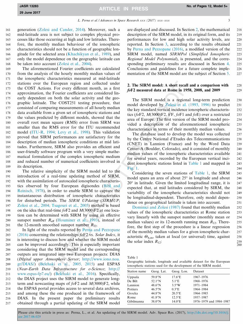
230The SIRM model is a regional long-term prediction231model developed by Zolesi et al. (1993, 1996) to predict232the key standard vertical incidence ionospheric characteris-233tics (foF2, M(3000)F2, h0F, foF1 and foE) over a restricted234area of Europe. The first version of the SIRM model pro-235vided a description of the aforementioned ionospheric236characteristics in terms of their monthly median values.237The database used to develop the model was collected238by the Centre National d’Etudes des Telecommunications239(CNET) in Lannion (France) and by the Word Data240Center-A (Boulder, Colorado), and it consisted of monthly241median values of the ionospheric characteristics available242for several years, recorded by the European vertical inci-243dent ionospheric stations listed in Table 1 and mapped in244Fig. 1.245Considering the seven stations of Table 1, the SIRM246model spans an area of about 25� in longitude and about24720� in latitude. Given the limited longitudinal range, it is248expected that, at mid latitudes considered by SIRM, the249variability of the ionospheric characteristics should not250be longitudinal-dependent. Therefore, only model depen-251dence on geographical latitude is taken into account.252Dominici and Zolesi (1987) found that monthly median253values of the ionospheric characteristics at Rome station254vary linearly with the sunspot number (monthly mean or255median values) or its 12-month running mean R12. There-256fore, the first step of the procedure is a linear regression257of the monthly median values for a given ionospheric char-258acteristic Hh,m, taken at local (or universal) time, against259the solar index R12:260

Table 1Geographic latitude, longitude and available dataset for the Europeanionospheric stations used for the development of the SIRM model.

Station name Geog. Lat. Geog. Lon. Dataset

Uppsala 59.8�N 17.6�E 1967–1976De Bilt 52.1�N 5.1�E 1968–1976Lannion 48.6�N 3.5�W 1971–1984Poitiers 46.5�N 0.3�E 1964–1984Grocka 44.8�N 20.5�E 1964–1985Rome 41.8�N 12.5�E 1957–1987Gibilmanna 38.0�N 14.0�E 1976–1979 and 1984–1987

L. Perna et al. / Advances in Space Research xxx (2017) xxx–xxx 3

JASR 13283 No. of Pages 12, Model 5+

29 June 2017

Please cite this article in press as: Perna, L., et al. An updating of the SIRM model. Adv. Space Res. (2017), http://dx.doi.org/10.1016/j.asr.2017.06.029

Hh;m ¼ ah;mðR12Þ þ bh;m: ð1Þ262262

263 In Eq. (1) ah,m and bh,m are two matrices of 288 coeffi-264 cients (24 h � 12 months), one for each hour (h) of the265 day, and for each month (m) of the year. Using Eq. (1),266 it is considered that the solar cycle variation of the monthly267 median values H can be fully described at any ionospheric268 station, for each month and hour, by only two levels of269 solar activity and the straight line joining them270 (McNamara, 1991). The linear regression analysis is then271 considered as the best prediction of the measured data at272 every single station. Two values of solar activity, R12 = 0273 and R12 = 100, are chosen and used to describe low and274 high solar activity levels, respectively, and two sets of syn-275 thetic monthly median values of the ionospheric character-276 istic H are then correspondingly obtained by using Eq. (1),277 for every station in question.278 The second step of the procedure consists of doing a279 Fourier analysis of the synthetic datasets obtained at the280 end of the first step:281

Hh;m ¼ A0 þXl

n

An sin2pntT

þ Y n

� �; ð2Þ

283283

284 where n is the harmonic number, T = 288 h corresponds to285 a fundamental period of a ‘‘virtual year” with a fixed level286 of R12, t is the time in hours for which t = 1 corresponds to287 00:00 LT of January and t = 288 to 23:00 LT of December.288 It is clear that with the coefficients A0, An and Yn, where289 n = 1, 2, . . ., l = 144, the Fourier synthesis repeats the H290 values that are obtained from Eq. (1) through the two

291matrices ah,m and bh,m. Zolesi et al. (1993, 1996) have292shown that A0 and 12 pairs (An, Yn) of dominant Fourier293coefficients are sufficient to reproduce the main features294of the diurnal, seasonal and solar cycle behaviour of the295mid-latitude ionosphere under quiet conditions. Using this296technique for every considered station (Table 1), Zolesi297et al. (1993) found a good agreement between the results298of the Fourier synthesis and the results of a simple linear299regression. In this way, it is possible to reproduce the tem-300poral variations of the key ionospheric characteristics at301each ionospheric station and, according to this evidence,302the Fourier coefficients A0, An and Yn in Eq. (2) can be con-303sidered, as a first approximation, linearly dependent on304R12:

305

A0 ¼ a0ðR12Þ þ b0;

An ¼ anðR12Þ þ bn;

Y n ¼ cnðR12Þ þ dn:

: ð3Þ307307

308Eq. (3) are applied to the database of the seven iono-309spheric stations shown in Fig. 1, using a local time (LT)310format and taking into account the differences between311LT and the local standard time through the phase Yn in312Eq. (2). Zolesi et al. (1993) found that the results for the313coefficients A0, An and Yn used in the evaluation of foF2,314M(3000)F2 and h’F, corresponding to R12 = 0 and315R12 = 100, show a linear variation with the geographic lat-316itude thus confirming the validity of the concept that the317coefficients a0, b0, an, bn, cn and dn, can be regarded as a lin-

Fig. 1. Map of European ionospheric stations used to develop the SIRM model.

4 L. Perna et al. / Advances in Space Research xxx (2017) xxx–xxx

JASR 13283 No. of Pages 12, Model 5+

29 June 2017

Please cite this article in press as: Perna, L., et al. An updating of the SIRM model. Adv. Space Res. (2017), http://dx.doi.org/10.1016/j.asr.2017.06.029

318 ear function of the geographic latitude / in a restricted319 area. Therefore, the spatial distribution of A0, An and Yn

320 can be expressed as:321

A0 ¼ ða10/þ a20ÞR12 þ b10/þ b20;

An ¼ ða1n/þ a2nÞR12 þ b1n/þ b2n;

Y n ¼ ðc1n/þ c2nÞR12 þ d1n/þ d2

n:

ð4Þ323323

324 The numerical coefficients aj0, b

j0, a

jn, b

jn, c

jn, d

jn with j = 1,

325 2 can be easily calculated by a linear regression of the326 Fourier coefficients of every ionospheric station versus327 their latitudes (Zolesi et al., 1990, 1991).328 The SIRM model is completely described by Eqs. (1)–329 (4). To fix the key points, the characteristics of the model330 are here summarized:

331 � Linear regressions between monthly median values Hh,m

332 and R12;333 � Consideration of two solar activity levels: R12 = 0 (low334 solar activity) and R12 = 100 (high solar activity). Other335 levels of solar activity are considered by a linear interpo-336 lation between these two boundaries;337 � Linear regressions between the Fourier coefficients A0,338 An and Yn and the R12 index;339 � Linear regressions between the Fourier coefficients A0,340 An and Yn and the latitude /;341 � No variations in longitude.342

343 As it was mentioned, it is important to underline how344 the total representation involves only 100 numerical coeffi-345 cients for each ionospheric characteristic and therefore346 yields considerable economy in data storage and347 computation.348 Preliminary results showed that the SIRM model foF2349 outputs match the input data used in their generation with350 a standard deviation of about 0.5 MHz (Zolesi et al., 1990).351 The reliability of the SIRM foF2 outputs have also been352 tested making comparisons with station measurements353 not used when generating the SIRM coefficients. For high354 solar activity, typical differences of around 0.7 MHz or less355 have been observed (Zolesi et al., 1991, 1993).356 Zolesi et al. (1996) have tested the SIRM performances357 with several inhomogeneous datasets from a sparse net-358 work of ionospheric stations in mid-latitude areas such as359 northeastern North America, southeastern South America,360 northeast Asia, and southeast Australia. The results show361 that the agreement between model and observed data for362 foF2 and M(3000)F2 is quite remarkable when taking into363 account simple assumptions, that is, no longitudinal-364 dependent variations, linear variation of the model coeffi-365 cients with the geographic latitude, and their reduced366 number.367 However, it is expected that for mid-latitude areas with368 a dense ionosondes network and continuous, long and reli-369 able datasets, such as the European region, SIRM outputs370 would provide very good agreements with observed data.371 In fact, due to its high-quality results in the European area,

372economy in computation and quick response, the SIRM373model and its real-time version SIRMUP, have been used374in the European project DIAS to produce long-term and375nowcasting maps of foF2 and M(3000)F2, which are also376accessed by the ESPAS portal.377As reported by Liu et al. (2011), the last solar minimum378has shown an unprecedented prolonged and low solar379activity, providing a perfect natural window to study the380ionospheric plasma response and the reliability of iono-381spheric models for such particular conditions. Therefore,382thanks to a very long, continuous and reliable dataset383available for the Rome station, it is very interesting to com-384pare the SIRM outputs with the Rome ionosonde monthly385median values, limiting the study to the most important386ionospheric characteristic foF2.387Figs. 2 and 3 report the comparison of hourly monthly388median values calculated by SIRM and measured by the389ionosonde at Rome, for 2008 and 2009, which represent390the deepest phase of the last solar minimum. SIRM outputs391provide good agreement with ionosonde data for both 2008392and 2009, using as input observed values of the solar index393R12. To quantify the SIRM performances, the mean devia-394tion ðPn

i¼1jfoF2SIRM � foF2obsji=nÞ has been calculated,395where foF2SIRM and foF2obs are monthly median foF2 val-396ues coming from SIRM and ionosonde, respectively. The397mean deviation values are 0.47 MHz and 0.43 MHz for398the whole 2008 and 2009 respectively, confirming the good399results provided by SIRM.400These results are not surprising because, as mentioned, it401is expected that SIRM model provides good correspon-402dences with ionosonde data in mid-latitude areas with a403dense ionosondes network. Furthermore, (1) Rome iono-404sonde data were used to develop the SIRM model (see

Fig. 2. Hourly monthly median foF2 values at the Rome station asmeasured by the ionosonde (black) and calculated by the SIRM model(dashed red) for the whole year 2008. The x axis spans from t = 0 (00:00LT of January 2008) to t = 288 (23:00 LT of December 2008). The capitalletters in blue identify the months from January (J) to December (D). (Forinterpretation of the references to colour in this figure legend, the reader isreferred to the web version of this article.)

L. Perna et al. / Advances in Space Research xxx (2017) xxx–xxx 5

JASR 13283 No. of Pages 12, Model 5+

29 June 2017

Please cite this article in press as: Perna, L., et al. An updating of the SIRM model. Adv. Space Res. (2017), http://dx.doi.org/10.1016/j.asr.2017.06.029

405 Table 1) and (2), as shown in Table 2, the R12 values for406 2008 and 2009 are very low and close to the value407 R12 = 0 that is one of the two levels of solar activity set408 in the model.409 However, Figs. 2 and 3 also show the following features:410 (1) the SIRM model tends to overestimate the daily peak of411 foF2, in particular for 2008; (2) night-time values are well412 described by the SIRM model during summer and spring413 months, while more pronounced differences characterize414 winter and autumn months (in particular January, Febru-415 ary, September and October).416 Moreover, we have to take into account that for mid417 and very high solar activity, the hysteresis and saturation418 effects (Kane, 1992; Mikhailov and Mikhailov, 1995; Liu419 et al., 2006; Rao and Rao, 1969; Triskova and Chum,420 1996) become important, in particular when foF2 vs. Solar421 Index relationships are considered using mean or median422 values, such as in the SIRM model. In particular, it was423 shown how the saturation can be viewed as a second order424 effect that, using linear regressions for foF2 vs. R12 rela-425 tionships, can lead to pronounced model overestimations426 (Perna and Pezzopane, 2016, and references therein).427 Fig. 4 shows a comparison between foF2 values calculated428 by SIRM and those recorded at Rome, for 1958, a year of

429very high solar activity (maximum of solar cycle 19, see430Table 2).431Contrary to 2008 and 2009, the year 1958 is included in432dataset used to develop the SIRM model (see Table 1),433therefore good results should be expected. This high solar434activity year has been chosen to test SIRM outputs,435because for all months the R12 value is markedly over the436saturation level, therefore it is expected that using the lin-437ear regression (1) pronounced overestimations can occur.438This is confirmed by the mean deviation between SIRM439and ionosonde values for the whole year 1958 which is4401.04 MHz, more than 50% higher than the results obtained441for 2008 and 2009. Furthermore, Fig. 4 shows that during442daytime hours for February, March, October, and Decem-443ber, SIRM overestimations as high as 3–4 MHz are444obtained.445As it was already mentioned, the simple formulation of446the SIRM model makes it easy to interface it with other447regional or global models. Moreover, the model can be also448used as a suitable tool to study the basic physical processes449controlling the behaviour of the F region and to provide a450quick prediction of ionospheric conditions (Belehaki et al.,4512005, 2015). For these reasons and in light of the results452shown in Figs. 2–4, it is interesting to test the results of a453partial updating of the SIRM model, named SIRMPol,454implemented according to the conclusions reported by455Perna and Pezzopane (2016) about the foF2 vs. Solar Index456relationship.

4573. The SIRMPol model: Main features

458Recent results about the foF2 vs. Solar Index relation-459ships (e.g., Liu et al., 2011; Chen et al., 2011; Perna and460Pezzopane, 2016) provide useful information to improve461the reliability of ionospheric models. In particular, the work462of Perna and Pezzopane (2016), concerning the very long,463continuous and reliable foF2 dataset of Rome ionosonde,464showed that: (1) the relationships foF2 vs. Solar Index can465be well described with a quadratic polynomial regression

Table 2R12 values for 2008, 2009 and 1958.

Month 2008 2009 1958

January 4.2 1.8 199.0February 3.6 1.9 200.9March 3.3 2.0 201.3April 3.4 2.2 196.8May 3.5 2.3 191.4June 3.3 2.7 186.8July 2.8 3.6 185.2August 2.7 4.8 184.9September 2.3 6.2 183.8October 1.8 7.1 182.2November 1.7 7.6 180.7December 1.7 8.3 180.5

Fig. 4. Same as Fig. 2 for 1958.Fig. 3. Same as Fig. 2 for 2009.

6 L. Perna et al. / Advances in Space Research xxx (2017) xxx–xxx

JASR 13283 No. of Pages 12, Model 5+

29 June 2017

Please cite this article in press as: Perna, L., et al. An updating of the SIRM model. Adv. Space Res. (2017), http://dx.doi.org/10.1016/j.asr.2017.06.029

466 for the mid-latitude station of Rome; (2) the use of linear fit-467 ting relationships (foF2 vs. Solar Index) gives rise to signifi-468 cant overestimations of observed data, because of both the469 saturation effect at high solar activity and the extremely470 low and prolonged solar activity like that characterizing471 the minimum between solar cycles 23 and 24.472 Accordingly, a first improvement that can be introduced473 in the SIRM model is to consider a second order polyno-474 mial regression for the relationship foF2 vs. R12:475

foF2h;m ¼ ah;mðR12Þ2 þ bh;mðR12Þ þ ch;m; ð5Þ477477

478 where the coefficients ah;m, bh;m and ch;m are calculated479 through a polynomial regression.480 The proposed update of the SIRM model, named481 SIRMPol (Simplified Ionospheric Regional Model Polyno-

482 mial), is based on very simple changes that can be summa-483 rized as follows:

484 1. The input dataset for Rome station has been updated,485 spanning from January 1957 to December 2007 (the486 SIRMmodel is based on the dataset for Rome from Jan-487 uary 1957 to December 1987). With regard to this, it is488 important to highlight that the dataset is composed by489 hourly validated values recorded from the 1st January490 1957 to the 31st December 2007, hence covering the solar491 cycles 19, 20, 21, 22, 23. The values were validated492 according to the International Union of Radio Science493 (URSI) standard (Wakai et al., 1987). The validation494 was performed from traces recorded by classical495 ionosondes, which cannot tag the different polarization496 characterizing the two different modes of propagation497 of the electromagnetic wave. A VOS-1 chirp ionosonde498 produced by the Barry Research Corporation, Palo Alto,499 CA, USA (Barry Research Corporation, 1975) sounded500 from January 1957 to November 2004, and then it was501 replaced by an AIS-INGV ionosonde (Zuccheretti502 et al., 2003), for which the ionograms were validated503 by using the Interpre software (Pezzopane, 2004). This504 means that the foF2 validated time series recorded at505 Rome represents a reliable and homogeneous dataset.506 Data were downloaded from the electronic Space507 Weather upper atmosphere database (eSWua; http://508 www.eswua.ingv.it/) (Romano et al., 2008).509 2. Nine synthetic foF2 datasets are constructed by consid-510 ering nine different values of solar activity: R12 = 0, 25,511 50, 75, 100, 125, 150, 175 and 200 (the SIRM model con-512 siders only two different values of R12: 0 and 100).513 3. A polynomial fit between the Fourier coefficients A0, An

514 and Yn and the solar index R12 is applied (a linear fit is515 instead applied by the SIRM model):

516517

A0 ¼ a0ðR12Þm þ b0ðR12Þm�1 þ . . .þ d;

An ¼ anðR12Þm þ bnðR12Þm�1 þ . . .þ c;

Y n ¼ cnðR12Þm þ dnðR12Þm�1 þ . . .þ m:

ð6Þ519519

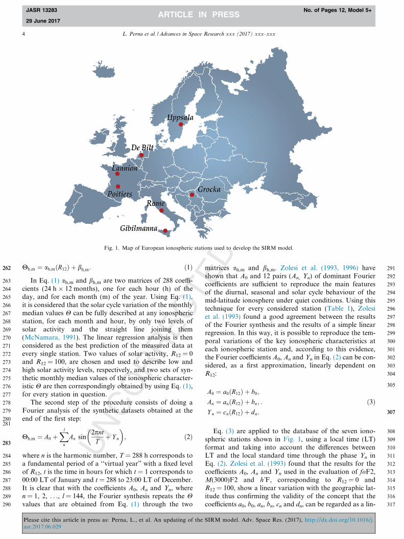
520Before showing the results of the SIRMPol model, it is521interesting to discuss, clarify and justify briefly the pro-522posed changes.523As a first consideration, it is worth noting that, owing to524a lack of data, it was not possible to consider the aforemen-525tioned changes for the other six ionosondes used to develop526the SIRM model (see Table 1). Consequently, the SIRM-527Pol model takes as input only data recorded at Rome528and then provides a description, in terms of foF2 monthly529median values, only for this station. Therefore, the updat-530ing proposed here has to be considered only a partial/local531updating of the SIRM model and can be considered a par-532ticular case of a single-station model. However, it is impor-533tant to underline that the main aim behind the534development of the SIRMPol model is to obtain useful535information to draft a list of guidelines for a future accu-536rate and complete updating of the SIRM model by addi-537tional ionospheric stations for which reliable datasets are538now available.539The choice of the second order polynomial regression540(Eq. (5)) should improve the reliability of outputs for high541solar activity levels, and for the very low solar activity542levels of the last solar minimum, according to what it543was shown by Perna and Pezzopane (2016). In support of544this, Fig. 5 shows scatterplots of foF2 vs. R12 for the Rome545dataset (1957–2007), for March, June, September and546December, at 01:00 LT and 13:00 LT. Red lines and blue547curves identify respectively a linear and a second order548regression of the dataset. Red dots represent values of the549last solar minimum (years 2008 and 2009) that are not550included in the fits. The figure shows how the saturation551effect presents a seasonal dependence, being more pro-552nounced in ionospheric spring-summer. However, this fea-553ture is well represented by a second order regression which,554at the same time, represents quite well the low values of the555last solar minimum.556To implement the SIRMPol model, nine levels of solar557activity have been considered from R12 = 0 to R12 = 200,558with a step of R12 = 25. This change should provide a bet-559ter representation of the ionospheric plasma for both levels560of solar activity between the two anchor points of the561SIRM model (R12 = 0 and R12 = 100) and high solar activ-562ity levels. Furthermore, considering nine values of R12, it563has been observed how the relations A0 vs. R12, An vs.564R12, and Yn vs. R12 are no more linear, as they are in the565SIRM model.566This is clearly shown in Fig. 6, where the relationships567A13 vs. R12 (black squares) and Y13 vs. R12 (blue squares)568are displayed. It is noticeable how the linear regressions569calculated on the basis of the only two values R12 = 0570and R12 = 100 (red lines), as it is done in the SIRM model,571are inadequate. In general, it has been concluded that, for572all the Fourier coefficients, polynomial (either second or573third order) regressions provide the best choice to represent574the relationships between Fourier coefficients and R12, as575indicated by the third-order polynomial regressions shown576in Fig. 6. It is worth noting that a test extending the series

L. Perna et al. / Advances in Space Research xxx (2017) xxx–xxx 7

JASR 13283 No. of Pages 12, Model 5+

29 June 2017

Please cite this article in press as: Perna, L., et al. An updating of the SIRM model. Adv. Space Res. (2017), http://dx.doi.org/10.1016/j.asr.2017.06.029

577 to 16 pairs (An, Yn) of dominant Fourier coefficients has578 not improved significantly the performances of SIRMPol.579 Therefore, as reported by Zolesi et al. (1993), it is con-

580firmed that 12 pairs (An, Yn) of dominant Fourier coeffi-581cients are sufficient to adequately describe the particular582ionospheric characteristic as it was the case in the SIRM583model.

5844. Results

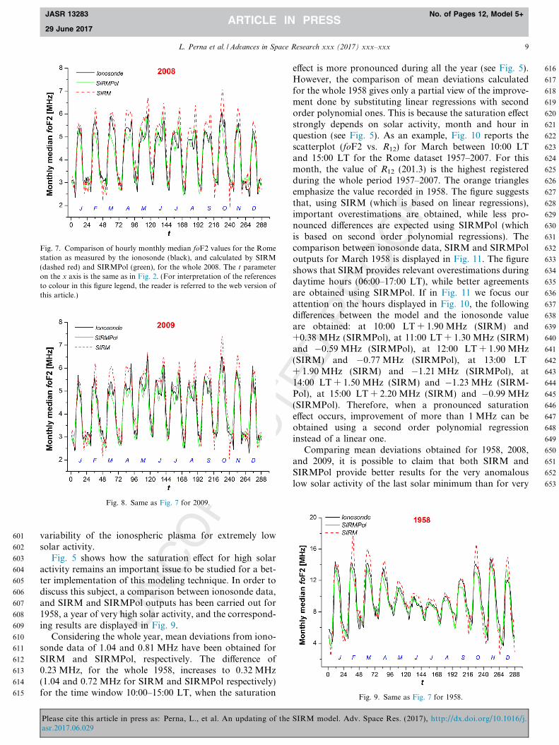
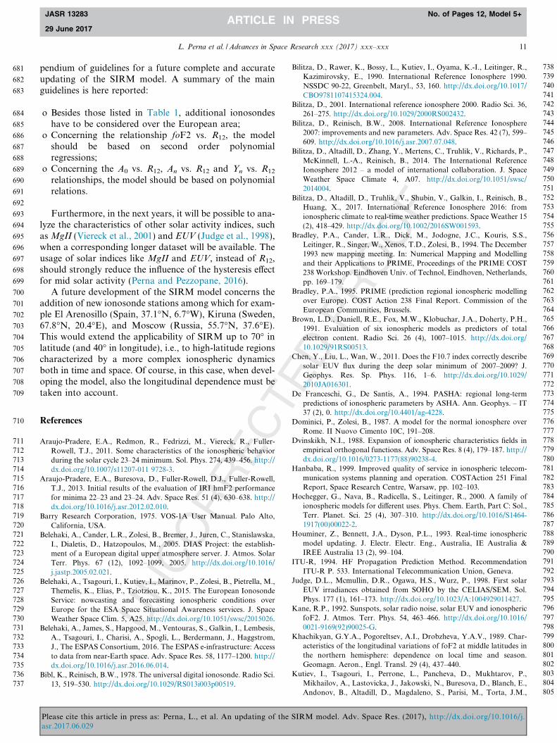
585Figs. 7 and 8 display the comparison of monthly median586foF2 values for the Rome station, as measured by the iono-587sonde, and calculated by SIRM and SIRMPol for 2008 and5882009, respectively. It is evident how, in some cases, the589SIRMPol provides a better agreement with ionosonde data590than the SIRM model. In particular, the SIRM tendency to591overestimate ionosonde values around midday appears592substantially reduced. Similarly, the SIRM underestima-593tions observed during night-time hours over January–594March and September–November periods result to be595reduced as well. Mean deviation values for the whole5962008 and 2009 reveal an improvement using SIRMPol,597from 0.47 MHz (SIRM) to 0.37 MHz (SIRMPol), for5982008, and from 0.43 MHz (SIRM) to 0.35 MHz (SIRM-599Pol), for 2009. Hence, it is confirmed that a second order600regression can be better than a linear one to express the

Fig. 5. Monthly mean foF2 vs. R12 at 01:00 LT and 13:00 LT for March, June, September, and December for the Rome dataset (1957–2007). The red lineand the blue curve represent respectively the linear and the second order polynomial regression. Red dots represent values for 2008 and 2009. (Forinterpretation of the references to colour in this figure legend, the reader is referred to the web version of this article.)

Fig. 6. A13 vs. R12 (black squares) and Y13 vs. R12 (blue squares) plots.Red lines represent linear regressions between the two points R12 = 0 andR12 = 100, as it is done in the SIRM model, while green curves representthird-order polynomial regressions. (For interpretation of the references tocolour in this figure legend, the reader is referred to the web version of thisarticle.)

8 L. Perna et al. / Advances in Space Research xxx (2017) xxx–xxx

JASR 13283 No. of Pages 12, Model 5+

29 June 2017

Please cite this article in press as: Perna, L., et al. An updating of the SIRM model. Adv. Space Res. (2017), http://dx.doi.org/10.1016/j.asr.2017.06.029

601 variability of the ionospheric plasma for extremely low602 solar activity.603 Fig. 5 shows how the saturation effect for high solar604 activity remains an important issue to be studied for a bet-605 ter implementation of this modeling technique. In order to606 discuss this subject, a comparison between ionosonde data,607 and SIRM and SIRMPol outputs has been carried out for608 1958, a year of very high solar activity, and the correspond-609 ing results are displayed in Fig. 9.610 Considering the whole year, mean deviations from iono-611 sonde data of 1.04 and 0.81 MHz have been obtained for612 SIRM and SIRMPol, respectively. The difference of613 0.23 MHz, for the whole 1958, increases to 0.32 MHz614 (1.04 and 0.72 MHz for SIRM and SIRMPol respectively)615 for the time window 10:00–15:00 LT, when the saturation

616effect is more pronounced during all the year (see Fig. 5).617However, the comparison of mean deviations calculated618for the whole 1958 gives only a partial view of the improve-619ment done by substituting linear regressions with second620order polynomial ones. This is because the saturation effect621strongly depends on solar activity, month and hour in622question (see Fig. 5). As an example, Fig. 10 reports the623scatterplot (foF2 vs. R12) for March between 10:00 LT624and 15:00 LT for the Rome dataset 1957–2007. For this625month, the value of R12 (201.3) is the highest registered626during the whole period 1957–2007. The orange triangles627emphasize the value recorded in 1958. The figure suggests628that, using SIRM (which is based on linear regressions),629important overestimations are obtained, while less pro-630nounced differences are expected using SIRMPol (which631is based on second order polynomial regressions). The632comparison between ionosonde data, SIRM and SIRMPol633outputs for March 1958 is displayed in Fig. 11. The figure634shows that SIRM provides relevant overestimations during635daytime hours (06:00–17:00 LT), while better agreements636are obtained using SIRMPol. If in Fig. 11 we focus our637attention on the hours displayed in Fig. 10, the following638differences between the model and the ionosonde value639are obtained: at 10:00 LT + 1.90 MHz (SIRM) and640+0.38 MHz (SIRMPol), at 11:00 LT + 1.30 MHz (SIRM)641and �0.59 MHz (SIRMPol), at 12:00 LT + 1.90 MHz642(SIRM) and �0.77 MHz (SIRMPol), at 13:00 LT643+ 1.90 MHz (SIRM) and �1.21 MHz (SIRMPol), at64414:00 LT + 1.50 MHz (SIRM) and �1.23 MHz (SIRM-645Pol), at 15:00 LT + 2.20 MHz (SIRM) and �0.99 MHz646(SIRMPol). Therefore, when a pronounced saturation647effect occurs, improvement of more than 1 MHz can be648obtained using a second order polynomial regression649instead of a linear one.650Comparing mean deviations obtained for 1958, 2008,651and 2009, it is possible to claim that both SIRM and652SIRMPol provide better results for the very anomalous653low solar activity of the last solar minimum than for very

Fig. 7. Comparison of hourly monthly median foF2 values for the Romestation as measured by the ionosonde (black), and calculated by SIRM(dashed red) and SIRMPol (green), for the whole 2008. The t parameteron the x axis is the same as in Fig. 2. (For interpretation of the referencesto colour in this figure legend, the reader is referred to the web version ofthis article.)

Fig. 8. Same as Fig. 7 for 2009.

Fig. 9. Same as Fig. 7 for 1958.

L. Perna et al. / Advances in Space Research xxx (2017) xxx–xxx 9

JASR 13283 No. of Pages 12, Model 5+

29 June 2017

Please cite this article in press as: Perna, L., et al. An updating of the SIRM model. Adv. Space Res. (2017), http://dx.doi.org/10.1016/j.asr.2017.06.029

654high solar activity. This feature needs to be further655investigated.

6565. Conclusions

657In this paper an updated version of the SIRM model,658called SIRMPol, was described and the corresponding659foF2 values have been compared with the ones recorded660at Rome mid-latitude ionospheric station, for years of661extremely high (1958) and low (2008 and 2009) solar662activity.663The main novelties introduced by the SIRMPol model664are: (1) an extension of the Rome ionosonde dataset (from6651957–1987 to 1957–2007); (2) the use of second order poly-666nomial regressions for the relations foF2 vs. R12 instead of667linear ones; (3) the consideration of nine levels of solar668activity instead of only two, and consequently the use of669polynomial relations to fit the relations A0 vs. R12, An vs.670R12 and Yn vs. R12 instead of linear ones. The obtained671results show that the SIRMPol foF2 outputs are better672than those of the SIRM model, specifically when a pro-673nounced saturation effect is observed at high solar activity.674Moreover, the outputs of both models are better for low675solar activity than for high solar activity.676It has to be noted that the SIRMPol model represents677only a partial updating of the SIRM model, because it pro-678vides outputs only for Rome ionospheric station and for679the characteristic foF2. However, the main aim of the680development of the SIRMPol model was to obtain a com-

Fig. 11. (Top) Comparison between hourly monthly median foF2 valuesobserved by the ionosonde (black), and calculated by SIRM (red) andSIRMPol (blue) for March 1958. The corresponding value of R12 is alsodisplayed. (Bottom) Point-to-point differences SIRM-Ionosonde (red) andSIRMPol-Ionosonde (blue). (For interpretation of the references to colourin this figure legend, the reader is referred to the web version of thisarticle.)

Fig. 10. foF2 vs. R12 for the Rome dataset (1957–2007) for March between 10:00 LT and 15:00 LT. Red lines and blue curves represent linear and secondorder polynomial regressions of the data. Orange triangles identify values for 1958. (For interpretation of the references to colour in this figure legend, thereader is referred to the web version of this article.)

10 L. Perna et al. / Advances in Space Research xxx (2017) xxx–xxx

JASR 13283 No. of Pages 12, Model 5+

29 June 2017

Please cite this article in press as: Perna, L., et al. An updating of the SIRM model. Adv. Space Res. (2017), http://dx.doi.org/10.1016/j.asr.2017.06.029

681 pendium of guidelines for a future complete and accurate682 updating of the SIRM model. A summary of the main683 guidelines is here reported:

684 o Besides those listed in Table 1, additional ionosondes685 have to be considered over the European area;686 o Concerning the relationship foF2 vs. R12, the model687 should be based on second order polynomial688 regressions;689 o Concerning the A0 vs. R12, An vs. R12 and Yn vs. R12

690 relationships, the model should be based on polynomial691 relations.692

693 Furthermore, in the next years, it will be possible to ana-694 lyze the characteristics of other solar activity indices, such695 as MgII (Viereck et al., 2001) and EUV (Judge et al., 1998),696 when a corresponding longer dataset will be available. The697 usage of solar indices like MgII and EUV, instead of R12,698 should strongly reduce the influence of the hysteresis effect699 for mid solar activity (Perna and Pezzopane, 2016).700 A future development of the SIRM model concerns the701 addition of new ionosonde stations among which for exam-702 ple El Arenosillo (Spain, 37.1�N, 6.7�W), Kiruna (Sweden,703 67.8�N, 20.4�E), and Moscow (Russia, 55.7�N, 37.6�E).704 This would extend the applicability of SIRM up to 70� in705 latitude (and 40� in longitude), i.e., to high-latitude regions706 characterized by a more complex ionospheric dynamics707 both in time and space. Of course, in this case, when devel-708 oping the model, also the longitudinal dependence must be709 taken into account.

710 References

711 Araujo-Pradere, E.A., Redmon, R., Fedrizzi, M., Viereck, R., Fuller-712 Rowell, T.J., 2011. Some characteristics of the ionospheric behavior713 during the solar cycle 23–24 minimum. Sol. Phys. 274, 439–456. http://714 dx.doi.org/10.1007/s11207-011 9728-3.715 Araujo-Pradere, E.A., Buresova, D., Fuller-Rowell, D.J., Fuller-Rowell,716 T.J., 2013. Initial results of the evaluation of IRI hmF2 performance717 for minima 22–23 and 23–24. Adv. Space Res. 51 (4), 630–638. http://718 dx.doi.org/10.1016/j.asr.2012.02.010.719 Barry Research Corporation, 1975. VOS-1A User Manual. Palo Alto,720 California, USA.721 Belehaki, A., Cander, L.R., Zolesi, B., Bremer, J., Juren, C., Stanislawska,722 I., Dialetis, D., Hatzopoulos, M., 2005. DIAS Project: the establish-723 ment of a European digital upper atmosphere server. J. Atmos. Solar724 Terr. Phys. 67 (12), 1092–1099, 2005. http://dx.doi.org/10.1016/725 j.jastp.2005.02.021.726 Belehaki, A., Tsagouri, I., Kutiev, I., Marinov, P., Zolesi, B., Pietrella, M.,727 Themelis, K., Elias, P., Tziotziou, K., 2015. The European Ionosonde728 Service: nowcasting and forecasting ionospheric conditions over729 Europe for the ESA Space Situational Awareness services. J. Space730 Weather Space Clim. 5, A25. http://dx.doi.org/10.1051/swsc/2015026.731 Belehaki, A., James, S., Hapgood, M., Ventouras, S., Galkin, I., Lembesis,732 A., Tsagouri, I., Charisi, A., Spogli, L., Berdermann, J., Haggstrom,733 J., The ESPAS Consortium, 2016. The ESPAS e-infrastructure: Access734 to data from near-Earth space. Adv. Space Res. 58, 1177–1200. http://735 dx.doi.org/10.1016/j.asr.2016.06.014.736 Bibl, K., Reinisch, B.W., 1978. The universal digital ionosonde. Radio Sci.737 13, 519–530. http://dx.doi.org/10.1029/RS013i003p00519.

738Bilitza, D., Rawer, K., Bossy, L., Kutiev, I., Oyama, K.-I., Leitinger, R.,739Kazimirovsky, E., 1990. International Reference Ionosphere 1990.740NSSDC 90-22, Greenbelt, Maryl., 53, 160. http://dx.doi.org/10.1017/741CBO9781107415324.004.742Bilitza, D., 2001. International reference ionosphere 2000. Radio Sci. 36,743261–275. http://dx.doi.org/10.1029/2000RS002432.744Bilitza, D., Reinisch, B.W., 2008. International Reference Ionosphere7452007: improvements and new parameters. Adv. Space Res. 42 (7), 599–746609. http://dx.doi.org/10.1016/j.asr.2007.07.048.747Bilitza, D., Altadill, D., Zhang, Y., Mertens, C., Truhlik, V., Richards, P.,748McKinnell, L.-A., Reinisch, B., 2014. The International Reference749Ionosphere 2012 – a model of international collaboration. J. Space750Weather Space Climate 4, A07. http://dx.doi.org/10.1051/swsc/7512014004.752Bilitza, D., Altadill, D., Truhlik, V., Shubin, V., Galkin, I., Reinisch, B.,753Huang, X., 2017. International Reference Ionosphere 2016: from754ionospheric climate to real-time weather predictions. Space Weather 15755(2), 418–429. http://dx.doi.org/10.1002/2016SW001593.756Bradley, P.A., Cander, L.R., Dick, M., Jodogne, J.C., Kouris, S.S.,757Leitinger, R., Singer, W., Xenos, T.D., Zolesi, B., 1994. The December7581993 new mapping meeting. In: Numerical Mapping and Modelling759and their Applications to PRIME, Proceedings of the PRIME COST760238 Workshop. Eindhoven Univ. of Technol, Eindhoven, Netherlands,761pp. 169–179.762Bradley, P.A., 1995. PRIME (prediction regional ionospheric modelling763over Europe). COST Action 238 Final Report. Commission of the764European Communities, Brussels.765Brown, L.D., Daniell, R.E., Fox, M.W., Klobuchar, J.A., Doherty, P.H.,7661991. Evaluation of six ionospheric models as predictors of total767electron content. Radio Sci. 26 (4), 1007–1015. http://dx.doi.org/76810.1029/91RS00513.769Chen, Y., Liu, L., Wan, W., 2011. Does the F10.7 index correctly describe770solar EUV flux during the deep solar minimum of 2007–2009? J.771Geophys. Res. Sp. Phys. 116, 1–6. http://dx.doi.org/10.1029/7722010JA016301.773De Franceschi, G., De Santis, A., 1994. PASHA: regional long-term774predictions of ionospheric parameters by ASHA. Ann. Geophys. – IT77537 (2), 0. http://dx.doi.org/10.4401/ag-4228.776Dominici, P., Zolesi, B., 1987. A model for the normal ionosphere over777Rome. II Nuovo Cimento 10C, 191–208.778Dvinskikh, N.I., 1988. Expansion of ionospheric characteristics fields in779empirical orthogonal functions. Adv. Space Res. 8 (4), 179–187. http://780dx.doi.org/10.1016/0273-1177(88)90238-4.781Hanbaba, R., 1999. Improved quality of service in ionospheric telecom-782munication systems planning and operation. COSTAction 251 Final783Report, Space Research Centre, Warsaw, pp. 102–103.784Hochegger, G., Nava, B., Radicella, S., Leitinger, R., 2000. A family of785ionospheric models for different uses. Phys. Chem. Earth, Part C: Sol.,786Terr. Planet. Sci. 25 (4), 307–310. http://dx.doi.org/10.1016/S1464-7871917(00)00022-2.788Houminer, Z., Bennett, J.A., Dyson, P.L., 1993. Real-time ionospheric789model updating. J. Electr. Electr. Eng., Australia, IE Australia &790IREE Australia 13 (2), 99–104.791ITU-R, 1994. HF Propagation Prediction Method. Recommendation792ITU-R P. 533. International Telecommunication Union, Geneva.793Judge, D.L., Mcmullin, D.R., Ogawa, H.S., Wurz, P., 1998. First solar794EUV irradiances obtained from SOHO by the CELIAS/SEM. Sol.795Phys. 177 (1), 161–173. http://dx.doi.org/10.1023/A:1004929011427.796Kane, R.P., 1992. Sunspots, solar radio noise, solar EUV and ionospheric797foF2. J. Atmos. Terr. Phys. 54, 463–466. http://dx.doi.org/10.1016/7980021-9169(92)90025-G.799Khachikyan, G.Y.A., Pogoreltsev, A.I., Drobzheva, Y.A.V., 1989. Char-800acteristics of the longitudinal variations of foF2 at middle latitudes in801the northern hemisphere: dependence on local time and season.802Geomagn. Aeron., Engl. Transl. 29 (4), 437–440.803Kutiev, I., Tsagouri, I., Perrone, L., Pancheva, D., Mukhtarov, P.,804Mikhailov, A., Lastovicka, J., Jakowski, N., Buresova, D., Blanch, E.,805Andonov, B., Altadill, D., Magdaleno, S., Parisi, M., Torta, J.M.,

L. Perna et al. / Advances in Space Research xxx (2017) xxx–xxx 11

JASR 13283 No. of Pages 12, Model 5+

29 June 2017

Please cite this article in press as: Perna, L., et al. An updating of the SIRM model. Adv. Space Res. (2017), http://dx.doi.org/10.1016/j.asr.2017.06.029

806 2013. Solar activity impact on the Earth’s upper atmosphere. J. Space807 Weather Space Climate 3, A06. http://dx.doi.org/10.1051/swsc/808 2013028.809 Levy, M.F., Dick, M.I., Spalla, P., Scotto, C., Kutiev, I., Muhtarov, P.,810 1998. Results of COST 251 testing of mappings and models. Rep.811 COST251TD(98)021, Eur. Coop. in the Field of Sci. and Tech. Res.,812 Brussels, Sept.813 Liu, L., Chen, Y., Le, H., 2006. Solar activity variations of the ionospheric814 peak electron density. J. Geophys. Res. Space Phys. 113, 1–13. http://815 dx.doi.org/10.1029/2008JA013114.816 Liu, L., Chen, Y., Le, H., Kurkin, V.I., Polekh, N.M., Lee, C.-C., 2011.817 The ionosphere under extremely prolonged low solar activity. J.818 Geophys. Res. Space Phys. 116, A04320. http://dx.doi.org/10.1029/819 2010JA016296.820 McNamara, L., 1991. The Ionosphere: Communications, Surveillance and821 Direction Finding. Krieger, Nalabar, Fla., p. 237.822 Mikhailov, A.V., Mikhailov, V.V., 1995. Solar cycle variations of annual823 mean noon foF2. Adv. Space Res. 15, 79–82. http://dx.doi.org/824 10.1016/S0273-1177(99)80026-X.825 Mikhailov, A.V., Mikhailov, V.V., Skoblin, M.G., 1996. Monthly median826 foF2 and M(3000)F2 ionospheric model over Europe. Ann. Geophys.827 – IT 39 (4), 791–805, http://hdl.handle.net/2122/1707.828 Mikhailov, A.V., Perrone, L., 2014. A method for foF2 short-term (1–24829 h) forecast using both historical and realtime foF2 observations over830 European stations: EUROMAP model. Radio Sci. 49, 253–270. http://831 dx.doi.org/10.1002/2014RS005373.832 Nava, B., Coisson, P., Radicella, S.M., 2008. A new version of the833 NeQuick ionosphere electron density model. J. Atmos Sol. Terr. Phys.834 70 (15), 1856–1862. http://dx.doi.org/10.1016/j.jastp.2008.01.015.835 Perna, L., Pezzopane, M., 2016. FoF2 vs solar indices for the Rome836 station: looking for the best general relation which is able to describe837 the anomalous minimum between cycles 23 and 24. J. Atmos. Sol.838 Terr. Phys. 148, 13–21. http://dx.doi.org/10.1016/j.jastp.2016.08.003.839 Pezzopane, M., 2004. Interpre: a windows software for semiautomatic840 scaling of ionospheric parameters from ionograms. Comput. Geosci.841 30, 125–130. http://dx.doi.org/10.1016/j.cageo.2003.09.009.842 Pezzopane, M., Pietrella, M., Pignatelli, A., Zolesi, B., Cander, L.R., 2011.843 Assimilation of autoscaled data and regional and local ionospheric844 models as input sources for real-time 3-D international reference845 ionosphere modeling. Radio Sci. 46, 5009. http://dx.doi.org/10.1029/846 2011RS004697.847 Pezzopane, M., Pietrella, M., Pignatelli, A., Zolesi, B., Cander, L.R., 2013.848 Testing the three-dimensional IRI-SIRMUP-P mapping of the iono-849 sphere for disturbed periods. Adv. Space Res. 52 (10), 1726–1736.850 http://dx.doi.org/10.1016/j.asr.2012.11.028.851 Pietrella, M., Perrone, L., 2005. Instantaneous space weighted ionospheric852 regional model for instantaneous mapping of the critical frequency of853 the F2 layer in the European region. Radio Sci. 40 (1). http://dx.doi.854 org/10.1029/2003RS003008.855 Pietrella, M., 2012. A short-term ionospheric forecasting empirical856 regional model (IFERM) to predict the critical frequency of the F2857 layer during moderate, disturbed, and very disturbed geomagnetic858 conditions over the European area. Ann. Geophys. 30, 343–355. http://859 dx.doi.org/10.5194/angeo-30-343-2012.860 Radicella, S.M., Leitinger, R., 2001. The evolution of the DGR approach861 to model electron density profiles. Adv. Space Res. 27 (1), 35–40.862 http://dx.doi.org/10.1016/S0273-1177(00)00138-1.863 Rao, M.S.J.G., Rao, R.S., 1969. The hysteresis variation in F2–layer864 parameters. J. Atmos. Terr. Phys. 31, 1119–1125. http://dx.doi.org/865 10.1016/0021- 9169(69)90110-X.

866Rawer, K., 1991. Data needed for an analytical description of the electron867density profile. Adv. Space Res. 11 (10), 57–65. http://dx.doi.org/86810.1016/0273-1177(91)90322-B.869Reinisch, B.W., Huang, X., Sales, G.S., 1993. Regional ionospheric870mapping. Adv. Space Res. 13 (3), 45–48. http://dx.doi.org/10.1016/8710273-1177(93)90246-8.872Romano, V., Pau, S., Pezzopane, M., Zuccheretti, E., Zolesi, B., De873Franceschi, G., Locatelli, S., 2008. The electronic space weather upper874atmosphere (eSWua) project at INGV: advancements and state of the875art. Ann. Geophys. 26, 345–351.876Singer, W., Dvinskikh, N.I., 1991. Comparison of empirical models of877ionospheric characteristics developed by means of different mapping878methods. Adv. Space Res. 11 (10), 3–6. http://dx.doi.org/10.1016/8790273-1177(91)90311-7.880Triskova, L., Chum, J., 1996. Hysteresis dependence of foF2 on solar881indices. Adv. Space Res. 18, 145–148. http://dx.doi.org/10.1016/0273-8821177(95)00915-9.883Tsagouri, I., Zolesi, B., Belehaki, A., Cander, L.R., 2005. Evaluation of884the performance of the real-time updated simplified ionospheric885regional model for the European area. J. Atm. Sol. Terr. Phys. 67886(12), 1137–1146. http://dx.doi.org/10.1016/j.jastp.2005.01.012.887Viereck, R., Puga, L., McMullin, D., Judge, D., Weber, M., Tobiska, W.888K., 2001. The Mg II index: a proxy for solar EUV. Geophys. Res. Lett.88928 (7), 1343–1346. http://dx.doi.org/10.1029/2000GL012551.890Wakai, N., Ohyama, H., Koizumi, T., 1987. Manual of Ionogram Scaling.891Ministry of posts and Telecommunications, Japan.892Zakharenkova, I., Krankowski, A., Bilitza, D., Cherniak, Y., Shagimu-893ratov, I., Sieradzki, R., 2013. Comparative study of foF2 measure-894ments with IRI-2007 model predictions during extended solar895minimum. Adv. Space Res. 51 (1), 620–629. http://dx.doi.org/89610.1016/j.asr.2011.11.015.897Zolesi, B., Cander, L.R., De Franceschi, G., 1990. A simple model for a898global distribution of some ionospheric characteristics in a restricted899area, in Solar-Terrestrial Predictions: Proceedings of a Workshop at900Leura, National Oceanic and Atmospheric Administration, Boulder,901Colo., vol. 2, pp. 418–427.902Zolesi, B., Cander, L.R., De Franceschi, G., 1991. Mapping of some903ionospheric characteristics over a restricted area using SIRM (Simpli-904fied Ionospheric Regional Model). In: Seventh International Confer-905ence on Antennas and Propagation, vol. 333, pp. 512–515.906Zolesi, B., Cander, L.R., De Franceschi, G., 1993. Simplified ionospheric907regional model for telecommunication applications. Radio Sci. 28 (4),908603–612. http://dx.doi.org/10.1029/93RS00276.909Zolesi, B., Cander, L.R., De Franceschi, G., 1996. On the potential910applicability of the simplified ionospheric regional model to different911midlatitude areas. Radio Sci. 31 (3), 547–552. http://dx.doi.org/91210.1029/95RS03817.913Zolesi, B., Cander, L.R., 1998. Advances in regional ionospheric mapping914over Europe. Ann. Geophys. – IT 41 (5–6), 827–842. http://dx.doi.org/91510.4401/ag-3823.916Zolesi, B., Belehaki, A., Tsagouri, I., Cander, L.R., 2004. Real-time917updating of the simplified ionospheric regional model for operational918applications. Radio Sci. 39 (2), RS2011. http://dx.doi.org/10.1029/9192003RS002936.920Zolesi, B., Cander, L.R., 2014. Ionospheric Prediction and Forecasting.921Springer-Verlag Berlin Heidelberg, p. 240. http://dx.doi.org/10.1007/922978-3-642-38430-1.923Zuccheretti, E., Tutone, G., Sciacca, U., Bianchi, C., Arokiasamy, B.J.,9242003. The new AIS-INGV digital ionosonde. Ann. Geophys. – IT 46925(4), 647–659. http://dx.doi.org/10.4401/ag-4377.

926

12 L. Perna et al. / Advances in Space Research xxx (2017) xxx–xxx

JASR 13283 No. of Pages 12, Model 5+

29 June 2017

Please cite this article in press as: Perna, L., et al. An updating of the SIRM model. Adv. Space Res. (2017), http://dx.doi.org/10.1016/j.asr.2017.06.029