Dealing with Uncertainties in Initial Orbit Determinationsites.utexas.edu/renato/files/2017/04/Paper.pdf · Dealing with Uncertainties in Initial Orbit Determination ... Renato Zanetti

Celestial Mechanics and Dynamical Astronomy manuscript No.(will be inserted by the editor)

Dealing with Uncertainties in Initial Orbit Determination

Roberto Armellin · Pierluigi Di Lizia ·Renato Zanetti

Received: date / Accepted: date

Abstract A method to deal with uncertainties in initial orbit determination(IOD) is presented. This is based on the use of Taylor differential algebra(DA) to nonlinearly map the observation uncertainties from the observationspace to the state space. When a minimum set of observations is available,DA is used to expand the solution of the IOD problem in Taylor series withrespect to measurement errors. When more observations are available, highorder inversion tools are exploited to obtain full state pseudo-observations ata common epoch. The mean and covariance of these pseudo-observations arenonlinearly computed by evaluating the expectation of high order Taylor poly-nomials. Finally, a linear scheme is employed to update the current knowledgeof the orbit. Angles-only observations are considered and simplified Kepleriandynamics adopted to ease the explanation. Three test cases of orbit determi-nation of artificial satellites in different orbital regimes are presented to discussthe feature and performances of the proposed methodology.

1 Introduction

Orbit determination is typically divided into two phases. When the numberof observation is equal to the number of unknowns, a nonlinear system ofequations need to be solved. This problem is known as initial (or preliminary)orbit determination (IOD). When more observations are available, accurate

Roberto ArmellinIEF Marie Sklodowska-Curie Fellow, Departamento de Matematicas y Computacion, Uni-versidad de La Rioja, 26006 Logrono, Spain ([email protected])Pierluigi Di LiziaAssistant Professor, Department of Aerospace Science and Technology, Politecnico di Mi-lano, 20156 Milan, Italy ([email protected])Renato ZanettiGN&C Engineer at NASA Johnson Space Center, 2101 NASA Road 1, Houston, Texas,77058, United States ([email protected])

2 Roberto Armellin et al.

orbit determination can be performed. IOD typically delivers a single solution(or a limited number of solutions) that exactly produces the available obser-vations. In addition, in IOD simplified dynamical models are often used (e.g.Keplerian motion) and measurement errors are not taken into account (theproblem is deterministic). When more observations are available the approachbecomes stochastic, because the additional observations include noise. Thisproblem is usually set as an optimization one, in which the (optimal) solutionis the one that minimizes the observation residuals. The solution is obtainedvia batch estimation, e.g. weighted nonlinear least squares, or a sequentialestimation, e.g. extended Kalman Filtering.1

In this paper we focus our attention on the orbit determination of residentspace objects (RSO) observed on a single passage with optical sensors. Thus,the problem is the one of an angles-only orbit determination. In order todetermine, the orbit an IOD problem is solved followed by a procedure toupdate the initial solution based on the additional observations.

Angles-only IOD is an old problem. Gauss’2 and Laplace’s3 methods arecommonly used to determine a Keplerian orbit that fits with three astromet-ric observations. These methods have been revisited and analyzed by a largenumber of authors (e.g. 4, 5, 6) and new ones introduced more recently. TheDouble r-iteration technique of Escobal7 and the approach of Gooding8 aretwo examples of angles-only methods introduced for the IOD of RSO.

In 2012 Armellin at al.9 proposed a IOD solver based on the solution ofa Lambert’s problem (between the second and the third observations) anda Kepler’s problem (between the first and second observation). The methoditerates on the slant ranges at the second and third observations in order todrive to zero the observational defects at the first observation. The iterationswere carried out with a high-order extension of Newton’s method enabledby differential algebra (DA). In addition, high order Taylor expansions wereexploited to nonlinearly map the uncertainties from the observation space tothe state space.

In this work a modified version of the method is proposed, in which all thethree slant ranges are the problem unknowns. The approach is based on thesolution of two Lambert’s problems and using the continuity of the velocityvector at the central observation as constraint. The method has no restrictionson the geometry of the observations and it can deal with both short andlong gaps. As in the previous work, the solution is obtained with a high-order Newton’s iteration scheme enabled by DA. This approach allows thealgorithm to both converge in few iterations and map uncertainties form theobservation space to the state space. Thus, the initial orbit is already providedwith statistical information.

When multiple observations on the same passage are available the IODsolution is updated. Instead of adopting a classical least squares approach(which employs the linearization of the dynamics and of the measurementfunctions10) high order inversion tools available in DA are exploited to nonlin-early map group of observations to the state space at a common epoch, thusproducing full state pseudo-observations. The mean and covariance of these

Dealing with Uncertainties in Initial Orbit Determination 3

pseudo-observations are nonlinearly computed by evaluating the expectationof the related high order Taylor polynomials. Finally, a linear updating schemeis utilized to update the current knowledge of the state mean and covariance.

The paper is organized as follows. A brief introduction on the DA tools usedfor the implementation of the algorithm is given first. This covers the meth-ods to expand the solution of ordinary differential equations (ODE), computethe expansion of the solution of parametric implicit equations, and the algo-rithm to map statistics through nonlinear transformations. The following sec-tions describe the main algorithms developed in this work, i.e. the angles-onlyIOD solver and the updating scheme. Simulated observational scenarios for aGeosynchronous Transfer Orbit (GTO), a Geosynchronous Orbit (GEO) anda Molniya are used to assess the performances of the implemented methods.Some final remarks conclude the paper.

2 Differential Algebra tools

DA supplies the tools to compute the derivatives of functions within a com-puter environment.11 More specifically, by substituting the classical imple-mentation of real algebra with the implementation of a new algebra of Taylorpolynomials, any function f of v variables is expanded into its Taylor polyno-mial up to an arbitrary order n with limited computational effort. In additionto basic algebraic operations, operations for differentiation and integration canbe easily introduced in the algebra, thusly finalizing the definition of the differ-ential algebra structure of DA.12,13 Similarly to algorithms for floating pointarithmetic, also in DA various algorithms were introduced, including methodsto perform composition of functions, to invert them, to solve nonlinear sys-tems explicitly, and to treat common elementary functions.14 The differentialalgebra used for the computations in this work was implemented in the soft-ware COSY INFINITY.15 The reader may refer to Di Lizia et al.16 for the DAnotation adopted throughout the paper.

2.1 High-order expansion of the solution of ODE

An important application of DA is the automatic high order expansion of thesolution of an ODE in terms of the initial conditions.14,16 This can be achievedby replacing the operations in a classical numerical integration scheme, includ-ing evaluation of the right hand side, by the corresponding DA operations.This way, starting from the DA representation of an initial condition x0, DAODE integration allows the propagation of the Taylor expansion of the flowin x0 forward in time, up to any final time tf . Any explicit ODE integrationscheme can be rewritten as a DA integration scheme in a straight-forward way.For the numerical integrations presented in this paper, a DA version of a 7/8Dormand-Prince (8-th order solution for propagation, 7-th order solution forstep size control) Runge-Kutta scheme is used. The main advantage of the


DA-based approach is that there is no need to write and integrate variationalequations in order to obtain high order expansions of the flow. It is thereforeindependent of the particular right hand side of the ODE and the method isquite efficient in terms of computational cost.

2.2 Expansion of the solution of parametric implicit equations

Well-established numerical techniques (e.g., Newton’s method) exist, whichcan effectively identify the solution of a classical implicit equation

f(x) = 0 (1)

with f : <n → <n. Suppose an explicit dependence on a vector of parametersp can be highlighted in the vector function f , which leads to the parametricimplicit equation

f(x,p) = 0. (2)

Suppose the above equation is to be solved, whose solution is represented bythe function x(p) returning the value of x solving (2) for any value of p. Thus,the dependence of the solution of the implicit equation on p is of interest.DA techniques can effectively handle the previous problem by identifying thefunction x(p) in terms of its Taylor expansion with respect to p. This resultis achieved by applying partial inversion techniques as detailed in 16.

The final result is

[x] = x+Mx(δp), (3)

which is the k-th order Taylor expansion of the solution of the implicit equa-tion. For every value of δp, the approximate solution of f(x,p) = 0 can beeasily computed by evaluating the Taylor polynomial (3). Apparently, the so-lution obtained by means of the polynomial map (3) is a Taylor approximationof the exact solution of Eq. (2). The accuracy of the approximation dependson both the order of the Taylor expansion and the displacement δp from thereference value of the parameter.

2.3 Nonlinear mapping of the estimate statistics

Consider a random variable x ∈ <n with probability density function p(x)and a second random variable y ∈ <m related to x through the nonlineartransformation

y = f(x). (4)

The problem is to calculate a consistent estimate of the main cumulants of thetransformed probability density function p(y). Since f is a generic nonlinearfunction, this formulation includes a wide range of problems involving un-certainty propagation (uncertainty propagation through nonlinear dynamics,uncertainty propagation through nonlinear coordinate transformations, etc.).


The Taylor expansion of y with respect to deviations δx can be obtainedautomatically by initializing the independent variable as a DA variable andevaluating (4) in DA framework. For each component yi of y, this proceduredelivers

[yi] = fi([x]) = yi +Myi(δx) =∑

p1+···+pn≤kci,p1...pn · δxp11 · · · δxpnn , (5)

where in this expression yi is the zeroth order term of the expansion map, andci,p1...pn are the Taylor coefficients of the resulting Taylor polynomial

ci,p1...pn =1

p1! · · · pn!· ∂

p1+···+pnfi∂xp11 · · · ∂xpnn

. (6)

The evaluation of (5) for a selected value of δx supplies the k-th order Taylorapproximation of yi corresponding to the displaced independent variable. Ofcourse, the accuracy of the expansion map is function of the expansion orderand can be controlled by tuning it.

The Taylor series in the form (5) can be used to efficiently compute thepropagated statistics.17,18 The method consists in analytically describing thestatistics of the solution by computing the l-th moment of the transformedpdf using a proper form of the l-th power of the solution map (5).

For a generic scalar random variable x with pdf p(x) the first four momentscan be written as

µ = ExP = E(x− µ)2γ =

E(x− µ)3σ3

κ =E(x− µ)4

σ4− 3,

(7)

where µ is the mean value, P is the covariance, σ is the standard deviation, γand κ are the skewness and the kurtosis, respectively,19 and the expectationvalue of x is defined as

Ex =

∫ +∞

−∞xp(x)dx. (8)

The moments of the transformed pdf in (4) can be computed by applyingthe multivariate form of Eq. (7) to the Taylor expansion (5). The result forthe first two moments becomesµyi = E[yi] =

∑p1+···+pn≤k

ci,p1...pnEδxp11 · · · δxpnn

P yiyj = E([yi]− µi)([yj ]− µj) =∑

p1+···+pn≤k,q1+···+qn≤k

ci,p1...pncj,q1...qnEδxp1+q11 · · · δxpn+qnn ,

(9)where ci,p1...pn are the Taylor coefficients of the Taylor polynomial describingthe i-th component of [y]. Note that in the covariance matrix formula the


coefficients ci,p1...pn and cj,q1...qn are updated to include the subtraction of themean. The coefficients of the higher order moments are computed by imple-menting the required operations (e.g. ([yi]−µi)([yj ]−µj) for the second ordermoment) on Taylor polynomials in the DA framework. The expectation valueson the right side of Eq. (9) are function of p(x). It follows that if the initialdistribution is known, all of the moments of the transformed pdf p(y) can becalculated. The number of monomials for which it is necessary to compute theexpectation increases with the order of the Taylor expansion and, of course,with the order of the moment we want to compute. Note that, at this time, nohypothesis on the initial pdf has been made. Thus, the method can be appliedindependently of the considered variable distribution.

We now consider the case in which x is a Gaussian random variable (GRV),x ∼ N (µ,P ), in which µ is the mean vector and P the covariance matrix. Animportant property of Gaussian distributions is that the statistics of a GRVcan be completely described by the first two moments. In case of zero mean,the expression for computing higher-order moments in terms of the covariancematrix is due to Isserlis.20 In physics literature, Isserlis’s formula is known asthe Wick’s formula.

Let s1 to sn be nonnegative integers, and s = s1 + s2 + · · ·+ sn. Then theWick’s formula suggests that

Exs11 xs22 . . . xsnn =

0, if s is odd

Haf(P ), if s is even(10)

where Haf(P ) is the hafnian of P = (σij), which is defined as

Haf(P ) =∑p∈∏s

s2∏i=1

σp2i−1,p2i , (11)

and∏s is the set of all permutations p of 1, 2, . . . , s satisfying the property

p1 < p3 < p5 < . . . < ps−1 and p1 < p2, p3 < p4, . . . , ps−1 < ps.21

We observe that the expectation value terms of Eq. (9) can be computedusing Eq. (10), and the resulting moments can be used to describe the trans-formed pdf.

3 DA-based angles-only IOD

In the classical angles-only IOD problem, three optical observations at epochti, with i = 1, . . . , 3 are available. The observations consist in three couplesof right ascension and declination angles, (αi, δi). These observations provideus with three inertial light of sights ρi, i.e. the unit vectors pointing from theobserver (on the Earth’s surface) to the observed object.

Assume to have first guess values of the slant ranges ρi or equivalently forthe orbit radii ri (e.g. from the solution of Gauss’ 8th degree polynomial). Wepresent a high order iterative procedure with the following objectives: a) refine


the values of ρi assuming Keplerian dynamics, and b) express the functionaldependence of the solution of the IOD problem with respect to observationuncertainties in terms of a high-order Taylor polynomials.

We start by initializing the observations as DA variables:

[α] = α+ δα[δ] = δ + δδ,

(12)

in which we have grouped the observations in two homogeneous vectors, α =(α1, α2, α3) and δ = (δ1, δ2, δ3), and δα and δδ accounts for measurementuncertainties. The line of sight vectors at t1, t2 and t3 become

[ρ1] = ρ1 +Mρ1(δα1, δδ1)

[ρ2] = ρ2 +Mρ2(δα2, δδ2)

[ρ3] = ρ3 +Mρ3(δα3, δδ3),

(13)

where Mρiis an arbitrary order Taylor polynomial that describes the effect

of an observation uncertainty on the line of sight.Similarly, we initialize DA variables on the topocentric distances at t1, t2

and t3[ρ1]1

−= ρ1

−

1 + δρ1[ρ2]1

−= ρ1

−

2 + δρ2[ρ3]1

−= ρ1

−

3 + δρ3,

(14)

or in more compact form

[ρ]1−

= ρ1−

+ δρ, (15)

where the superscript 1− indicates the first step of the iterative procedure,and ρ1

−

1 , ρ1−

2 , and ρ1−

3 are the guess values for the slant ranges.The spacecraft position vectors can be written (by summing the known

observer’s locations) as

[r1] = r1 +Mr1(δα1, δδ1, δρ1)[r2] = r2 +Mr2(δα2, δδ2, δρ2)[r3] = r3 +Mr3(δα3, δδ3, δρ3).

(16)

A DA-based Lambert’s problem22 can be solved between [r1] and [r2], andbetween [r2] and [r3]. Using the DA-implementation of Lambert’s problem weobtain two polynomial approximations for the velocity vector at t2

[v−2 ] = v−2 +Mv−2

(δα1, δδ1, δα2, δδ2, δρ1, δρ2)

[v+2 ] = v+2 +Mv+2

(δα2, δδ2, δα3, δδ3, δρ2, δρ3)(17)

Note that the above expressions of the velocity vector are different for tworeasons. First, the starting values of the slant ranges are not the solution ofthe IOD problem; secondly, they have different functional dependence on theobservation angles. The goal is thus a) to find the values of the slant rangessuch that the velocity vector is continuos at the midpoint, i.e., we want to


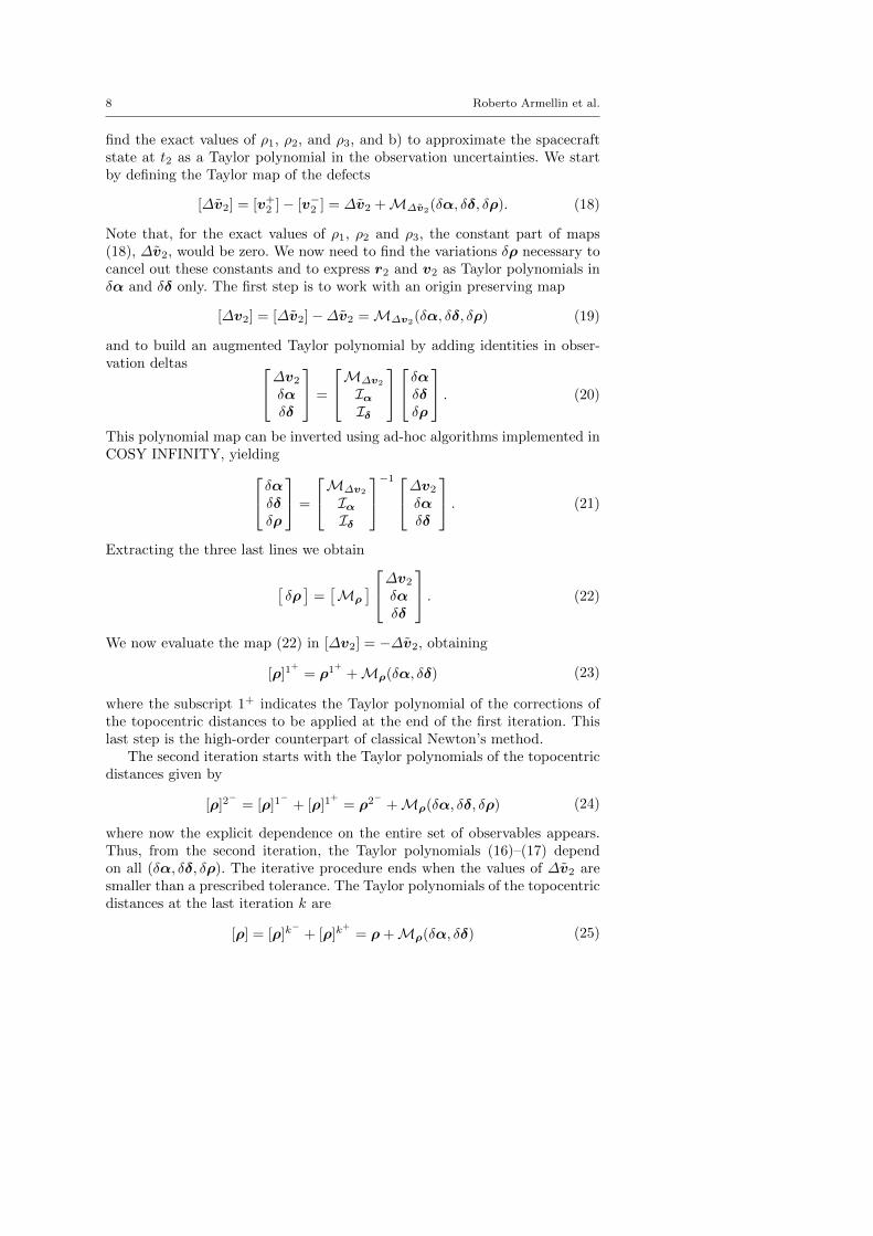
find the exact values of ρ1, ρ2, and ρ3, and b) to approximate the spacecraftstate at t2 as a Taylor polynomial in the observation uncertainties. We startby defining the Taylor map of the defects

[∆v2] = [v+2 ]− [v−2 ] = ∆v2 +M∆v2(δα, δδ, δρ). (18)

Note that, for the exact values of ρ1, ρ2 and ρ3, the constant part of maps(18), ∆v2, would be zero. We now need to find the variations δρ necessary tocancel out these constants and to express r2 and v2 as Taylor polynomials inδα and δδ only. The first step is to work with an origin preserving map

[∆v2] = [∆v2]−∆v2 =M∆v2(δα, δδ, δρ) (19)

and to build an augmented Taylor polynomial by adding identities in obser-vation deltas ∆v2δα

δδ

=

M∆v2

IαIδ

δαδδδρ

. (20)

This polynomial map can be inverted using ad-hoc algorithms implemented inCOSY INFINITY, yielding δαδδ

δρ

=

M∆v2

IαIδ

−1 ∆v2δαδδ

. (21)

Extracting the three last lines we obtain

[δρ]

=[Mρ

] ∆v2δαδδ

. (22)

We now evaluate the map (22) in [∆v2] = −∆v2, obtaining

[ρ]1+

= ρ1+

+Mρ(δα, δδ) (23)

where the subscript 1+ indicates the Taylor polynomial of the corrections ofthe topocentric distances to be applied at the end of the first iteration. Thislast step is the high-order counterpart of classical Newton’s method.

The second iteration starts with the Taylor polynomials of the topocentricdistances given by

[ρ]2−

= [ρ]1−

+ [ρ]1+

= ρ2−

+Mρ(δα, δδ, δρ) (24)

where now the explicit dependence on the entire set of observables appears.Thus, from the second iteration, the Taylor polynomials (16)–(17) dependon all (δα, δδ, δρ). The iterative procedure ends when the values of ∆v2 aresmaller than a prescribed tolerance. The Taylor polynomials of the topocentricdistances at the last iteration k are

[ρ] = [ρ]k−

+ [ρ]k+

= ρ+Mρ(δα, δδ) (25)


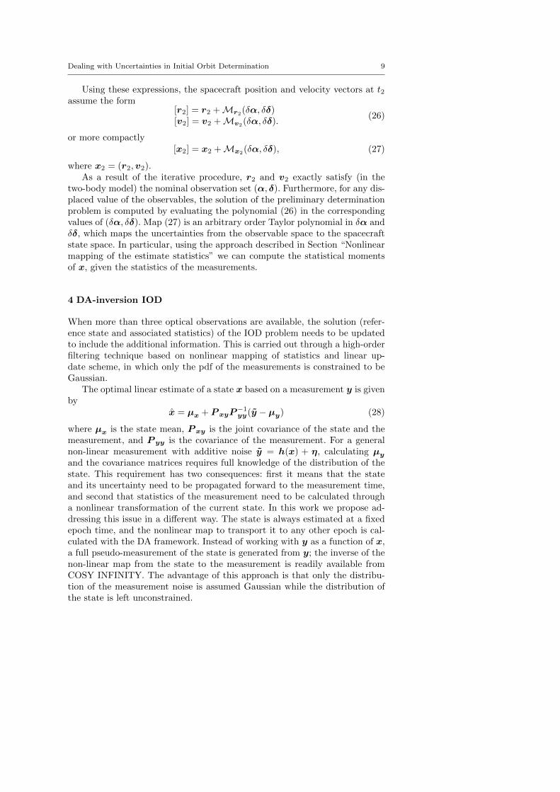
Using these expressions, the spacecraft position and velocity vectors at t2assume the form

[r2] = r2 +Mr2(δα, δδ)[v2] = v2 +Mv2(δα, δδ).

(26)

or more compactly[x2] = x2 +Mx2

(δα, δδ), (27)

where x2 = (r2,v2).As a result of the iterative procedure, r2 and v2 exactly satisfy (in the

two-body model) the nominal observation set (α, δ). Furthermore, for any dis-placed value of the observables, the solution of the preliminary determinationproblem is computed by evaluating the polynomial (26) in the correspondingvalues of (δα, δδ). Map (27) is an arbitrary order Taylor polynomial in δα andδδ, which maps the uncertainties from the observable space to the spacecraftstate space. In particular, using the approach described in Section “Nonlinearmapping of the estimate statistics” we can compute the statistical momentsof x, given the statistics of the measurements.

4 DA-inversion IOD

When more than three optical observations are available, the solution (refer-ence state and associated statistics) of the IOD problem needs to be updatedto include the additional information. This is carried out through a high-orderfiltering technique based on nonlinear mapping of statistics and linear up-date scheme, in which only the pdf of the measurements is constrained to beGaussian.

The optimal linear estimate of a state x based on a measurement y is givenby

x = µx + P xyP−1yy(y − µy) (28)

where µx is the state mean, P xy is the joint covariance of the state and themeasurement, and P yy is the covariance of the measurement. For a generalnon-linear measurement with additive noise y = h(x) + η, calculating µyand the covariance matrices requires full knowledge of the distribution of thestate. This requirement has two consequences: first it means that the stateand its uncertainty need to be propagated forward to the measurement time,and second that statistics of the measurement need to be calculated througha nonlinear transformation of the current state. In this work we propose ad-dressing this issue in a different way. The state is always estimated at a fixedepoch time, and the nonlinear map to transport it to any other epoch is cal-culated with the DA framework. Instead of working with y as a function of x,a full pseudo-measurement of the state is generated from y; the inverse of thenon-linear map from the state to the measurement is readily available fromCOSY INFINITY. The advantage of this approach is that only the distribu-tion of the measurement noise is assumed Gaussian while the distribution ofthe state is left unconstrained.


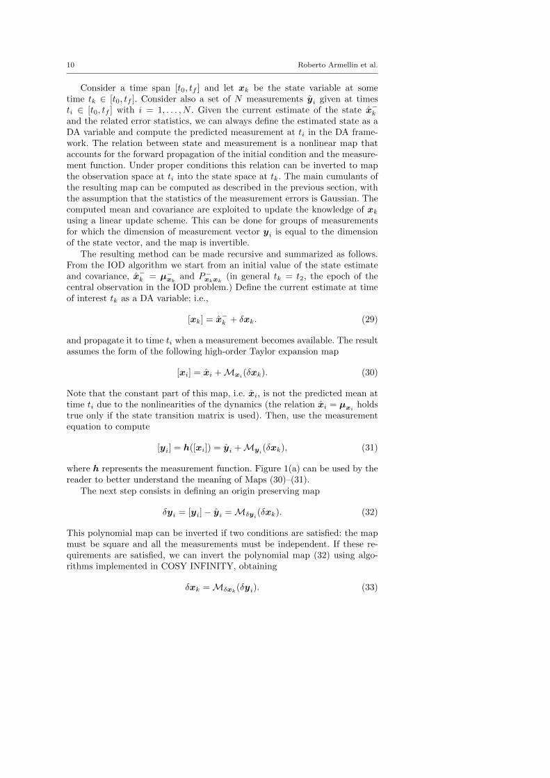
Consider a time span [t0, tf ] and let xk be the state variable at sometime tk ∈ [t0, tf ]. Consider also a set of N measurements yi given at timesti ∈ [t0, tf ] with i = 1, . . . , N . Given the current estimate of the state x−kand the related error statistics, we can always define the estimated state as aDA variable and compute the predicted measurement at ti in the DA frame-work. The relation between state and measurement is a nonlinear map thataccounts for the forward propagation of the initial condition and the measure-ment function. Under proper conditions this relation can be inverted to mapthe observation space at ti into the state space at tk. The main cumulants ofthe resulting map can be computed as described in the previous section, withthe assumption that the statistics of the measurement errors is Gaussian. Thecomputed mean and covariance are exploited to update the knowledge of xkusing a linear update scheme. This can be done for groups of measurementsfor which the dimension of measurement vector yi is equal to the dimensionof the state vector, and the map is invertible.

The resulting method can be made recursive and summarized as follows.From the IOD algorithm we start from an initial value of the state estimateand covariance, x−k = µ−xk

and P−xkxk(in general tk = t2, the epoch of the

central observation in the IOD problem.) Define the current estimate at timeof interest tk as a DA variable; i.e.,

[xk] = x−k + δxk. (29)

and propagate it to time ti when a measurement becomes available. The resultassumes the form of the following high-order Taylor expansion map

[xi] = xi +Mxi(δxk). (30)

Note that the constant part of this map, i.e. xi, is not the predicted mean attime ti due to the nonlinearities of the dynamics (the relation xi = µxi

holdstrue only if the state transition matrix is used). Then, use the measurementequation to compute

[yi] = h([xi]) = yi +Myi(δxk), (31)

where h represents the measurement function. Figure 1(a) can be used by thereader to better understand the meaning of Maps (30)–(31).

The next step consists in defining an origin preserving map

δyi = [yi]− yi =Mδyi(δxk). (32)

This polynomial map can be inverted if two conditions are satisfied: the mapmust be square and all the measurements must be independent. If these re-quirements are satisfied, we can invert the polynomial map (32) using algo-rithms implemented in COSY INFINITY, obtaining

δxk =Mδxk(δyi). (33)


δxk

δyi

x−k xi +Mxi

(δxk)xi

yi

yi +Myi(δxk)

(a) Direct maps representation

yi

x−k

yi

y i− y i

x−k+M z k

(δy i)

µzk

zk

zk − µzk

(b) Inverse map representation

Fig. 1: Sketch of the Taylor maps involved in the construction of the DA-basemap inversion nonlinear filter.

We now replace δxk in (29) with its expression from (33), yielding

[xk] = x−k +Mxk(δyi). (34)

This map now represents the pseudo-measurement of state xk based on theobservation yi, so it is renamed as

[zk] = x−k +Mzk(δyi). (35)

By construction the constant part of Eq. (35) is equal to the state estimateat step k, i.e. x−k , but its statistical moments are different to those of xk, dueto the nonlinear contribution of Mzk

(δyi) (as highlighted in Fig. 1(b)). Wecan now apply Eq. (9) to Taylor expansion (35) to compute the statistics of therandom variable zk and, in particular, the first two moments µzk

and P zkzk.

The computed mean can be treated as the “predicted measure” of the state attime tk, with measurement error defined by P zkzk

. Thus, we can update theinitial estimate and error covariance, using the least squares method. This canbe done using the Kalman filter update equations that, applied to the currentproblem, read

K =P−xkxk

(P−xkxk

+ P zkzk

)−1, (36)

x+k =x−k +K

(zk − µzk

), (37)

P+xkxk

= (I −K)P−xkxk(I −K)

T+KP zkzk

KT , (38)

where x+k is the updated estimate at time tk and P+

xkxkthe related updated

covariance matrix. When another measurement becomes available, we can de-fine the state at time tk as a new DA variable, centered in the new estimatex+k , and iterate the process. Note that zk is the true state-measurement at

ti mapped to time tk, which is readily available by evaluating Map (35) forδyi = yi − yi.

We said that the polynomial map in Eq. (32) must be square in order to beinvertible. It follows that if the measurement vector has smaller dimension thanthe state vector, after the first measurement is received we can not proceed


with the update, but we have to wait for additional measurements (i.e. inthe optical case three observations are needed). When the number of scalarmeasurements equals the dimension of the state variable, we can define anaugmented measurement vector that can be used to build Maps (31) and (32).

Once the final estimate of the state at time tk is obtained, the statisticsof the solution can be computed at any time via propagation and DA-basedexpectation evaluation.

5 Test Cases

The algorithms for IOD are run considering single-pass optical observations ofthree objects as listed in Table 1.

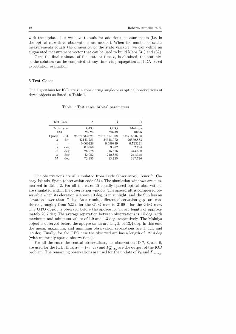
Table 1: Test cases: orbital parameters

Test Case A B C

Orbit type GEO GTO MolniyaSSC 26824 23238 40296

Epoch JED 2457163.2824 2457167.1008 2457165.0708a km 42143.781 24628.972 26569.833e – 0.000226 0.699849 0.723221i deg 0.0356 3.962 62.794Ω deg 26.278 315.676 344.538ω deg 42.052 240.885 271.348M deg 72.455 13.735 347.726

The observations are all simulated from Teide Observatory, Tenerife, Ca-nary Islands, Spain (observation code 954). The simulation windows are sum-marized in Table 2. For all the cases 15 equally spaced optical observationsare simulated within the observation window. The spacecraft is considered ob-servable when its elevation is above 10 deg, is in sunlight, and the Sun has anelevation lower than -7 deg. As a result, different observation gaps are con-sidered, ranging from 522 s for the GTO case to 2160 s for the GEO case.The GTO object is observed before the apogee for an arc length of approxi-mately 20.7 deg. The average separation between observations is 1.5 deg, withmaximum and minimum values of 1.9 and 1.3 deg, respectively. The Molniyaobject is observed before the apogee on an arc length of 13.4 deg. In this casethe mean, maximum, and minimum observation separations are 1, 1.1, and0.8 deg. Finally, for the GEO case the observed arc has a length of 127.4 deg(with uniformly spaced observations).

For all the cases the central observations, i.e. observation ID 7, 8, and 9,are used for the IOD; thus, x8 = (r8, v8) and P−x8,x8

are the output of the IODproblem. The remaining observations are used for the update of x8 and P−x8,x8

.


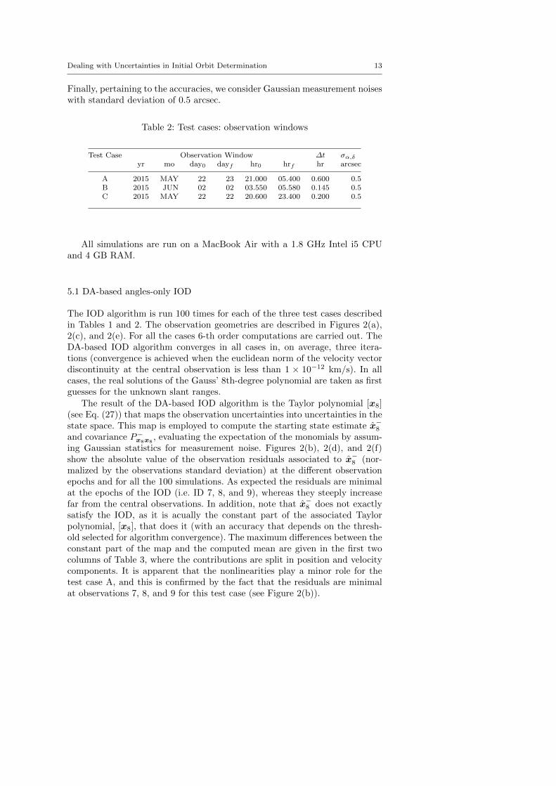
Finally, pertaining to the accuracies, we consider Gaussian measurement noiseswith standard deviation of 0.5 arcsec.

Table 2: Test cases: observation windows

Test Case Observation Window ∆t σα,δyr mo day0 dayf hr0 hrf hr arcsec

A 2015 MAY 22 23 21.000 05.400 0.600 0.5B 2015 JUN 02 02 03.550 05.580 0.145 0.5C 2015 MAY 22 22 20.600 23.400 0.200 0.5

All simulations are run on a MacBook Air with a 1.8 GHz Intel i5 CPUand 4 GB RAM.

5.1 DA-based angles-only IOD

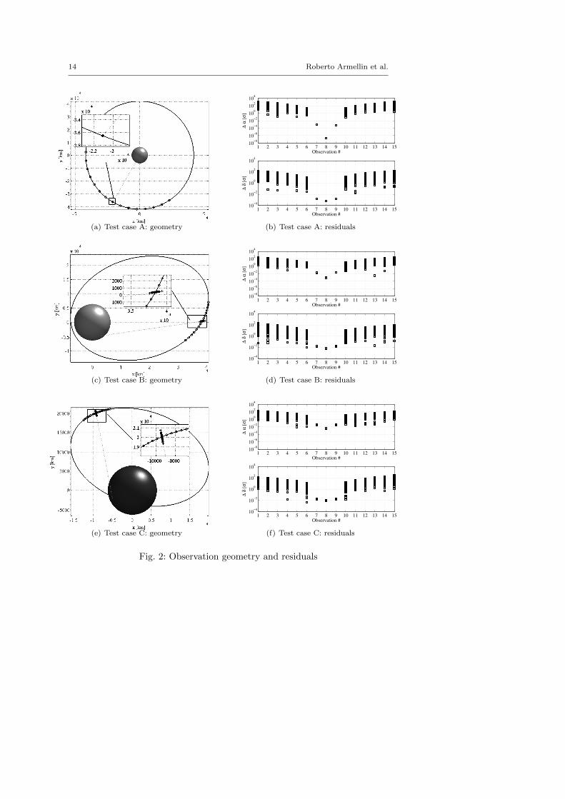
The IOD algorithm is run 100 times for each of the three test cases describedin Tables 1 and 2. The observation geometries are described in Figures 2(a),2(c), and 2(e). For all the cases 6-th order computations are carried out. TheDA-based IOD algorithm converges in all cases in, on average, three itera-tions (convergence is achieved when the euclidean norm of the velocity vectordiscontinuity at the central observation is less than 1 × 10−12 km/s). In allcases, the real solutions of the Gauss’ 8th-degree polynomial are taken as firstguesses for the unknown slant ranges.

The result of the DA-based IOD algorithm is the Taylor polynomial [x8](see Eq. (27)) that maps the observation uncertainties into uncertainties in thestate space. This map is employed to compute the starting state estimate x−8and covariance P−x8x8

, evaluating the expectation of the monomials by assum-ing Gaussian statistics for measurement noise. Figures 2(b), 2(d), and 2(f)show the absolute value of the observation residuals associated to x−8 (nor-malized by the observations standard deviation) at the different observationepochs and for all the 100 simulations. As expected the residuals are minimalat the epochs of the IOD (i.e. ID 7, 8, and 9), whereas they steeply increasefar from the central observations. In addition, note that x−8 does not exactlysatisfy the IOD, as it is acually the constant part of the associated Taylorpolynomial, [x8], that does it (with an accuracy that depends on the thresh-old selected for algorithm convergence). The maximum differences between theconstant part of the map and the computed mean are given in the first twocolumns of Table 3, where the contributions are split in position and velocitycomponents. It is apparent that the nonlinearities play a minor role for thetest case A, and this is confirmed by the fact that the residuals are minimalat observations 7, 8, and 9 for this test case (see Figure 2(b)).


(a) Test case A: geometry

1 2 3 4 5 6 7 8 9 10 11 12 13 14 1510

−8

10−6

10−4

10−2

100

102

104

Observation #

∆ α

[σ

]

1 2 3 4 5 6 7 8 9 10 11 12 13 14 1510

−4

10−2

100

102

104

Observation #

∆ δ

[σ

]

(b) Test case A: residuals

(c) Test case B: geometry

1 2 3 4 5 6 7 8 9 10 11 12 13 14 1510

−8

10−6

10−4

10−2

100

102

104

Observation #

∆ α

[σ

]

1 2 3 4 5 6 7 8 9 10 11 12 13 14 1510

−4

10−2

100

102

104

Observation #

∆ δ

[σ

]

(d) Test case B: residuals

(e) Test case C: geometry

1 2 3 4 5 6 7 8 9 10 11 12 13 14 1510

−8

10−6

10−4

10−2

100

102

104

Observation #

∆ α

[σ

]

1 2 3 4 5 6 7 8 9 10 11 12 13 14 1510

−4

10−2

100

102

104

Observation #

∆ δ

[σ

]

(f) Test case C: residuals

Fig. 2: Observation geometry and residuals


In all the cases the estimated covariance P−x8x8is stretched along the line of

sight directions as shown in the zoomed portions of Figures 2(a), 2(c), and 2(e).Higher nonlinearities affect test cases B and C, for which the uncertainty set ismuch more stretched. To quantify this, the maximum of the square root of theposition and velocity covariance matrix eigenvalues (indicated with maxσr8and maxσv8

) are reported in Table 3.

Table 3: IOD: uncertainty set description.

Test Case max ||r8 − r−8 || max ||v8 − v−

8 || maxσr8 maxσv8

km m/s km m/s

A 0.045 0.003 26.528 1.976B 7.579 0.349 340.993 14.611C 22.435 1.312 573.765 30.675

5.2 DA-based inversion IOD

The results obtained by applying the updating scheme presented in Sec. “DA-inversion IOD” are presented in this section. 100 simulations are run for eachtest case and all the computations are carried out at order 6, as for the DA-based IOD.

As we are considering 15 equally spaced optical observations, the maximumnumber of iterations (including the IOD using observations 7, 8, and 9) is 5.The updating scheme is stopped whenever the maximum number of iterationis reached or when the variation in the estimated state gets bigger than 5 timesthe maximum eigenvalues of the starting state covariance (this is consideredas an anomaly in the updating scheme).

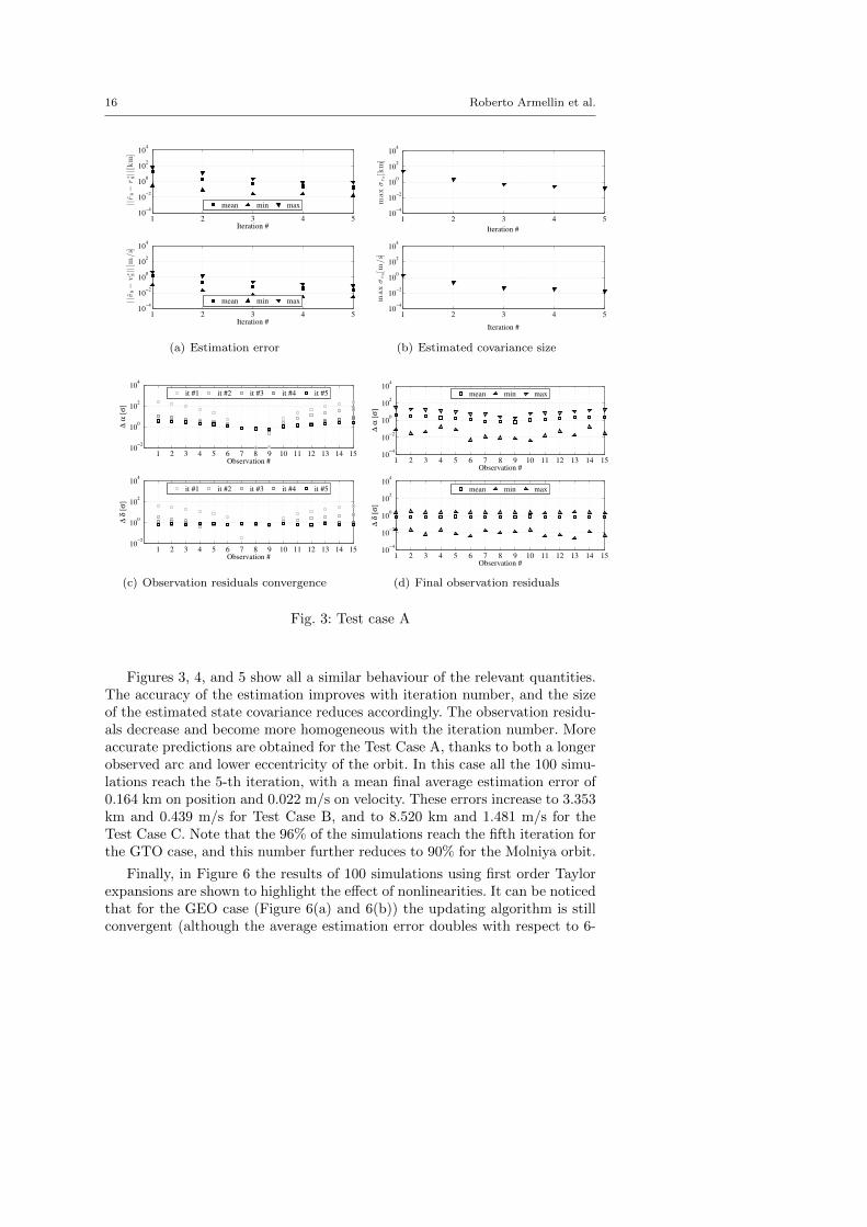
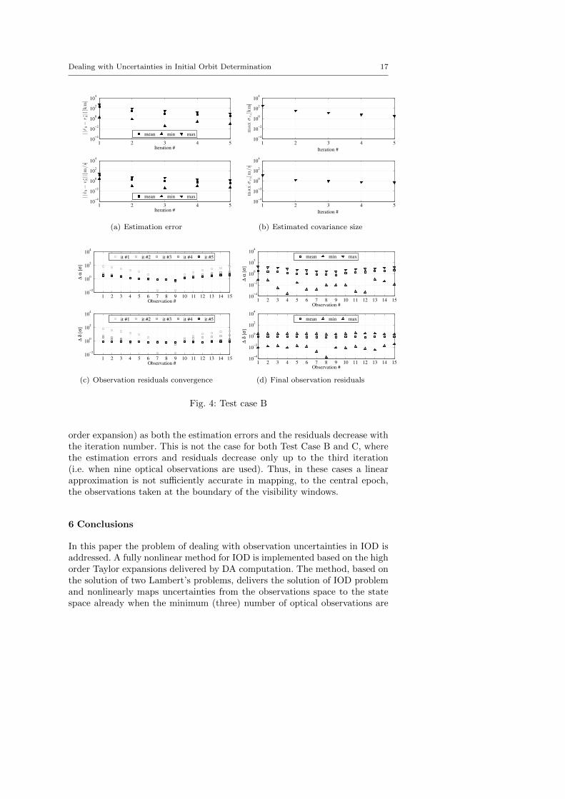
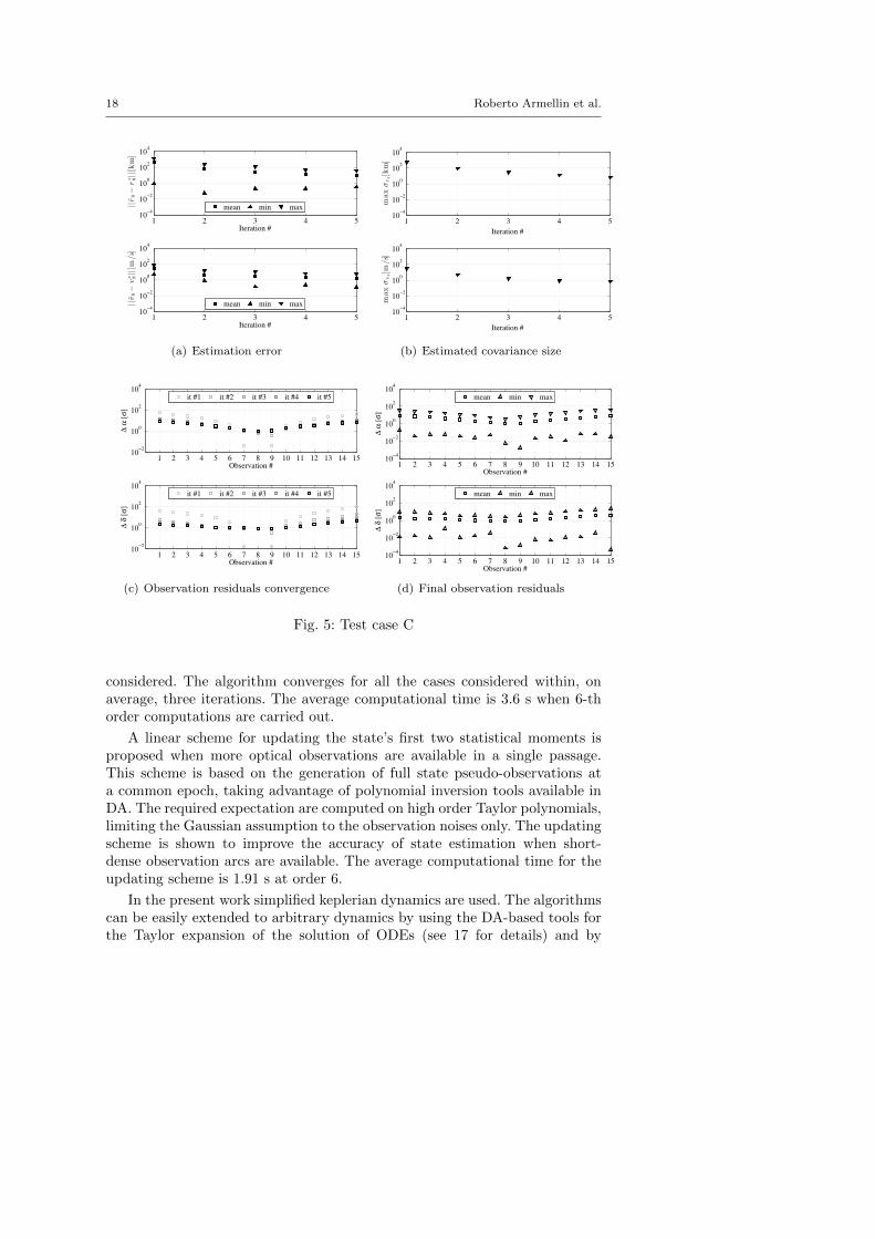
For all the cases a set of 4 plots is presented. In the first one the differencebetween the current state estimate and the true state (indicated as ||r8 − r∗8||for position and ||v8 − v∗8|| for velocity) is plotted as function of the iterationnumber. Mean, maximum and minimum values for the considered 100 simu-lations are shown with different markers. In the second figure the maximum(over the 100 simulations) of the maximum position and velocity eigenvaluesof the estimated covariance matrix are plotted as a function of the iterationnumber. Thus, the first two figures can be used to extract informations on stateaccuracy estimation and size of the estimated final uncertainty set. The thirdand fourth figures are about the observations residuals. More specifically, inthe third figure the evolution of the mean residuals with the iteration numberis highlighted using markers in gray scale (black markers for the last iteration);whereas in the fourth figure we plot the mean, maximum, and minimum valuesof the residuals (absolute value) at the the fifth iteration only.


1 2 3 4 510

−4

10−2

100

102

104

Iteration #

||r8−

r∗ 8||[km]

mean min max

1 2 3 4 510

−4

10−2

100

102

104

Iteration #

||v8−

v∗ 8||[m

/s]

mean min max

(a) Estimation error

1 2 3 4 510

−4

10−2

100

102

104

Iteration #

maxσr8[km]

1 2 3 4 510

−4

10−2

100

102

104

Iteration #

maxσv8[m

/s]

(b) Estimated covariance size

1 2 3 4 5 6 7 8 9 10 11 12 13 14 1510

−2

100

102

104

Observation #

∆ α

[σ

]

1 2 3 4 5 6 7 8 9 10 11 12 13 14 1510

−2

100

102

104

Observation #

∆ δ

[σ

]

it #1 it #2 it #3 it #4 it #5

it #1 it #2 it #3 it #4 it #5

(c) Observation residuals convergence

1 2 3 4 5 6 7 8 9 10 11 12 13 14 1510

−4

10−2

100

102

104

Observation #

∆ α

[σ

]

1 2 3 4 5 6 7 8 9 10 11 12 13 14 1510

−4

10−2

100

102

104

Observation #

∆ δ

[σ

]

mean min max

mean min max

(d) Final observation residuals

Fig. 3: Test case A

Figures 3, 4, and 5 show all a similar behaviour of the relevant quantities.The accuracy of the estimation improves with iteration number, and the sizeof the estimated state covariance reduces accordingly. The observation residu-als decrease and become more homogeneous with the iteration number. Moreaccurate predictions are obtained for the Test Case A, thanks to both a longerobserved arc and lower eccentricity of the orbit. In this case all the 100 simu-lations reach the 5-th iteration, with a mean final average estimation error of0.164 km on position and 0.022 m/s on velocity. These errors increase to 3.353km and 0.439 m/s for Test Case B, and to 8.520 km and 1.481 m/s for theTest Case C. Note that the 96% of the simulations reach the fifth iteration forthe GTO case, and this number further reduces to 90% for the Molniya orbit.

Finally, in Figure 6 the results of 100 simulations using first order Taylorexpansions are shown to highlight the effect of nonlinearities. It can be noticedthat for the GEO case (Figure 6(a) and 6(b)) the updating algorithm is stillconvergent (although the average estimation error doubles with respect to 6-


1 2 3 4 510

−4

10−2

100

102

104

Iteration #

||r8−

r∗ 8||[km]

mean min max

1 2 3 4 510

−4

10−2

100

102

104

Iteration #

||v8−

v∗ 8||[m

/s]

mean min max


1 2 3 4 510

−4

10−2

100

102

104

Iteration #

maxσr8[km]

1 2 3 4 510

−4

10−2

100

102

104

Iteration #

maxσv8[m

/s]


1 2 3 4 5 6 7 8 9 10 11 12 13 14 1510

−2

100

102

104

Observation #

∆ α

[σ

]

1 2 3 4 5 6 7 8 9 10 11 12 13 14 1510

−2

100

102

104

Observation #

∆ δ

[σ

]

it #1 it #2 it #3 it #4 it #5

it #1 it #2 it #3 it #4 it #5


1 2 3 4 5 6 7 8 9 10 11 12 13 14 1510

−4

10−2

100

102

104

Observation #

∆ α

[σ

]

1 2 3 4 5 6 7 8 9 10 11 12 13 14 1510

−4

10−2

100

102

104

Observation #

∆ δ

[σ

]

mean min max

mean min max


Fig. 4: Test case B

order expansion) as both the estimation errors and the residuals decrease withthe iteration number. This is not the case for both Test Case B and C, wherethe estimation errors and residuals decrease only up to the third iteration(i.e. when nine optical observations are used). Thus, in these cases a linearapproximation is not sufficiently accurate in mapping, to the central epoch,the observations taken at the boundary of the visibility windows.

6 Conclusions

In this paper the problem of dealing with observation uncertainties in IOD isaddressed. A fully nonlinear method for IOD is implemented based on the highorder Taylor expansions delivered by DA computation. The method, based onthe solution of two Lambert’s problems, delivers the solution of IOD problemand nonlinearly maps uncertainties from the observations space to the statespace already when the minimum (three) number of optical observations are


1 2 3 4 510

−4

10−2

100

102

104

Iteration #

||r8−

r∗ 8||[km]

mean min max

1 2 3 4 510

−4

10−2

100

102

104

Iteration #

||v8−

v∗ 8||[m

/s]

mean min max


1 2 3 4 510

−4

10−2

100

102

104

Iteration #

maxσr8[km]

1 2 3 4 510

−4

10−2

100

102

104

Iteration #

maxσv8[m

/s]


1 2 3 4 5 6 7 8 9 10 11 12 13 14 1510

−2

100

102

104

Observation #

∆ α

[σ

]

1 2 3 4 5 6 7 8 9 10 11 12 13 14 1510

−2

100

102

104

Observation #

∆ δ

[σ

]

it #1 it #2 it #3 it #4 it #5

it #1 it #2 it #3 it #4 it #5


1 2 3 4 5 6 7 8 9 10 11 12 13 14 1510

−4

10−2

100

102

104

Observation #

∆ α

[σ

]

1 2 3 4 5 6 7 8 9 10 11 12 13 14 1510

−4

10−2

100

102

104

Observation #

∆ δ

[σ

]

mean min max

mean min max


Fig. 5: Test case C

considered. The algorithm converges for all the cases considered within, onaverage, three iterations. The average computational time is 3.6 s when 6-thorder computations are carried out.

A linear scheme for updating the state’s first two statistical moments isproposed when more optical observations are available in a single passage.This scheme is based on the generation of full state pseudo-observations ata common epoch, taking advantage of polynomial inversion tools available inDA. The required expectation are computed on high order Taylor polynomials,limiting the Gaussian assumption to the observation noises only. The updatingscheme is shown to improve the accuracy of state estimation when short-dense observation arcs are available. The average computational time for theupdating scheme is 1.91 s at order 6.

In the present work simplified keplerian dynamics are used. The algorithmscan be easily extended to arbitrary dynamics by using the DA-based tools forthe Taylor expansion of the solution of ODEs (see 17 for details) and by


1 2 3 4 510

−4

10−2

100

102

104

Iteration #

||r8−

r∗ 8||[km]

mean min max

1 2 3 4 510

−4

10−2

100

102

104

Iteration #

||v8−

v∗ 8||[m

/s]

mean min max

(a) Estimation error (Test Case A)

1 2 3 4 5 6 7 8 9 10 11 12 13 14 1510

−2

100

102

104

Observation #

∆ α

[σ

]

1 2 3 4 5 6 7 8 9 10 11 12 13 14 1510

−2

100

102

104

Observation #

∆ δ

[σ

]

it #1 it #2 it #3 it #4 it #5

it #1 it #2 it #3 it #4 it #5

(b) Observation residuals convergence (TestCase A)

1 2 3 4 510

−4

10−2

100

102

104

Iteration #

||r8−

r∗ 8||[km]

mean min max

1 2 3 4 510

−4

10−2

100

102

104

Iteration #

||v8−

v∗ 8||[m

/s]

mean min max

(c) Estimation error (Test Case B)

1 2 3 4 5 6 7 8 9 10 11 12 13 14 1510

−2

100

102

104

Observation #

∆ α

[σ

]

1 2 3 4 5 6 7 8 9 10 11 12 13 14 1510

−2

100

102

104

Observation #

∆ δ

[σ

]

it #1 it #2 it #3 it #4 it #5

it #1 it #2 it #3 it #4 it #5

(d) Observation residuals convergence (TestCase B)

1 2 3 4 510

−4

10−2

100

102

104

Iteration #

||r8−

r∗ 8||[km]

mean min max

1 2 3 4 510

−4

10−2

100

102

104

Iteration #

||v8−

v∗ 8||[m

/s]

mean min max

(e) Estimation error (Test Case C)

1 2 3 4 5 6 7 8 9 10 11 12 13 14 1510

−2

100

102

104

Observation #

∆ α

[σ

]

1 2 3 4 5 6 7 8 9 10 11 12 13 14 1510

−2

100

102

104

Observation #

∆ δ

[σ

]

it #1 it #2 it #3 it #4 it #5

it #1 it #2 it #3 it #4 it #5

(f) Observation residuals convergence (TestCase C)

Fig. 6: Update results for 1st order computations


replacing the Lambert’s solver with a DA-based algorithm for expanding thesolution of two-point boundary values problems (as illustrated in 16). Theauthors plan to apply the algorithms to real observations including the caseof short-dense radar observations.

Acknowledgements R. Armellin acknowledges the support received by the Sklodowska-Curie grant 627111 (HOPT - Merging Lie perturbation theory and Taylor Differential algebrato address space debris challenges).

References

1. D. A. Vallado and W. D. McClain, Fundamentals of astrodynamics and applications,Vol. 12. Springer Science & Business Media, 2001.

2. C. F. Gauss and C. H. Davis, Theory of the Motion of the Heavenly Bodies Movingabout the Sun in Conic Sections. Courier Corporation, 2004.

3. P. Laplace, “Memoires de l’Academie Royale des Sciences,” Paris, Reprinted inLaplace’s Collected Works, Vol. 10, 1780.

4. G. Merton, “A modification of Gauss’s method for the determination of orbits,” MonthlyNotices of the Royal Astronomical Society, Vol. 85, 1925, p. 693.

5. A. Celletti and G. Pinzari, “Dependence on the observational time intervals and domainof convergence of orbital determination methods,” Periodic, Quasi-Periodic and ChaoticMotions in Celestial Mechanics: Theory and Applications, pp. 327–344, Springer, 2006.

6. G. F. Gronchi, “Multiple solutions in preliminary orbit determination from three obser-vations,” Celestial Mechanics and Dynamical Astronomy, Vol. 103, No. 4, 2009, pp. 301–326.

7. P. R. Escobal, “Methods of orbit determination,” New York: Wiley, 1965, Vol. 1, 1965.8. R. Gooding, “A new procedure for the solution of the classical problem of minimal orbit

determination from three lines of sight,” Celestial Mechanics and Dynamical Astron-omy, Vol. 66, No. 4, 1996, pp. 387–423.

9. R. Armellin, P. Di Lizia, and M. Lavagna, “High-order expansion of the solution of pre-liminary orbit determination problem,” Celestial Mechanics and Dynamical Astronomy,Vol. 112, No. 3, 2012, pp. 331–352.

10. O. Montebruck and E. Gill, Satellite Orbits. New York: Springer-Verlag, 2nd ed., 2001.11. M. Berz, Differential Algebraic Techniques, Entry in Handbook of Accelerator Physics

and Engineering. New York: World Scientific, 1999a.12. M. Berz, The new method of TPSA algebra for the description of beam dynamics to

high orders. Los Alamos National Laboratory, 1986. Technical Report AT-6:ATN-86-16.13. M. Berz, “The method of power series tracking for the mathematical description of

beam dynamics,” Nuclear Instruments and Methods A258, 1987.14. M. Berz, Modern Map Methods in Particle Beam Physics. Academic Press, 1999b.15. M. Berz and K. Makino, COSY INFINITY version 9 reference manual. Michigan State

University, East Lansing, MI 48824, 2006. MSU Report MSUHEP060803.16. P. Di Lizia, R. Armellin, and M. Lavagna, “Application of high order expansions of two-

point boundary value problems to astrodynamics,” Celestial Mechanics and DynamicalAstronomy, Vol. 102, No. 4, 2008, pp. 355–375.

17. M. Valli, R. Armellin, P. Di Lizia, and M. Lavagna, “Nonlinear mapping of uncertaintiesin celestial mechanics,” Journal of Guidance, Control, and Dynamics, Vol. 36, No. 1,2012, pp. 48–63.

18. R. Park and D. Scheeres, “Nonlinear Mapping of Gaussian Statistics: theory and Appli-cations to Spacecraft trajectory Design,” Journal of Guidance, Control and Dynamics,Vol. 29, No. 6, 2006.

19. G. Casella and R. Berger, Statistical inference. Duxbury Press, 2001.20. L. Isserlis, “On a formula for the product-moment coefficient of any order of a normal

frequency distribution in any number of variables,” Biometrika, Vol. 12, No. 1 and 2,1918.


21. R. Kan, “From moments of sum to moments of product,” Journal of Multivariate Anal-ysis, Vol. 99, No. 3, 2008.

22. R. Armellin, P. Di Lizia, F. Topputo, M. Lavagna, F. Bernelli-Zazzera, and M. Berz,“Gravity assist space pruning based on differential algebra,” Celestial mechanics anddynamical astronomy, Vol. 106, No. 1, 2010, pp. 1–24.

Documents

Dealing with Uncertainties in Initial Orbit Determinationsites.utexas.edu/renato/files/2017/04/Paper.pdf · Dealing with Uncertainties in Initial Orbit Determination ... Renato Zanetti