DEA PRICING SYSTEM

Journal of the Operations Research Society of Japan

Vol. 40, No. 2, June 1997

DEA PRICING SYSTEM

Toshiyuki Sueyoshi Science University of Tokyo

(Received October 23, 1995; Revised November 13, 1996)

Abstract This research presents a new application of Data Envelopment Analysis (DEA) to empirically determine prices of multiple products. The DEA technique is now widely applied to performance analysis and efficiency measurement in economics, business and other areas in social science. This study does not explore such conventional DEA uses, rather directing towards a new DEA application to the determination of a marginal cost pricing system or a profit-based pricing system. Nonlinear properties of the new DEA approach are explored in this research.

1. Introduction Data Envelopment Analysis, first proposed by Charnes et al. (1978), is now widely applied to performance (productivity) analysis and efficiency measurement in public and private sectors. The DEA applicability can be easily confirmed in the bibliography prepared by Seiford (1996) in which this study can find more than 500 previous DEA research efforts, including Sueyoshi (1991, 1992a,b,c, 1994).

Admitting the importance of such previous DEA contributions in efficiency analysis, this article needs to mention that DEA can serve as an empirical basis for determining market prices of multiple commodities. Unfortunately, such type of DEA applications have been not sufficiently explored in the conventional studies. [Exceptions may be found in Sueyoshi (1995c, 1996c).] To extend DEA further into a pricing mechanism, this article incorporates important economic concepts regarding pricing policy (e.g., a demand curve, an equilibrium market price, and market competition) into an DEA algorithmic framework. Thus, this research attempts to explore how a market price is determined in the DEA framework. [This article believes that DEA price-setting issue is as important as its traditional efficiency and productivity measurement. This article is a small but important step of such a new DEA research direct ion .]

The remaining structure of this article is organized as follows: The next (2) section reviews DEA from the perspective of its efficiency measurement. Section 3 discusses how DEA can be incorporated into a pricing mechanism. Nonlinear properties of an DEA pricing scheme are discussed in this section, as well. DEA pricing rule and efficiency concepts are presented in Section 4. After applying the proposed DEA approach to an illustrative data set, the next section (5) discusses the importance of the DEA-based pricing approach. Finally, conclusion and future research extensions are summarized in the last (6) section.

2. Traditional DEA Models DEA has been long considered as a data-oriented approach for relatively evaluating the performance of a group of entities referred to as "Decision Making Units (DMus)". In the DEA framework, DMus are regarded as decisional entities responsible for converting

© 1997 The Operations Research Society of Japan

DEA Pricing System 221

multiple inputs to outputs. Examples of such DMus include local authority departments, schools, hospitals, shops, bank branches, and other entities whose production activities are characterized by multiple inputs-outputs.

The original DEA model, first referred to as "CCR-ratio form" (Charnes et al., 1978), has opened up a new nonparametric scheme for the measurement of production-based efficiency. An important feature of DEA is that it promises analytical advantages in a case of the absence of need for the assignment of the supposed relative importance of various outputs and inputs. DEA also eliminates the need to explicitly specify underlying functional relationship that is supposed to analytically prescribe the relationship between inputs and outputs, as found in conventional parametric studies.

Hereafter, to initiate our mathematical description on the conventional use of DEA, this article starts with an assumption that there are n DMus, denoted by j E J = {j 1 j = l, 2, - - - , n}. The production process of each DMU is further characterized by an input (column) vector X, = (xi,, x2j, , xm,lT > 0 to produce an output (column) vector

Yi = ( Y l j , y2ji * , ysj}^ > 0. Here, the superscript "T" indicates a vector transpose. [For research convenience, this article excludes a case in which some components of the input and/or output vectors are zeros.] This model is now further extended to many different types of DEA formulations. Among these many DEA models, this article employs the following one to estimate the level of production-based efficiency on the specific kth DMU (Tone, 1993):

Minimize 6 n

subject to - x x j \ , + 6 X k > o ,

j= 1

A j > 0, and 6 > 0,

where A, ( j = 1, - - , n) is used to express a convex ball for connecting all the data points (X,, Y,} and its sum is restricted by its upper (ub 2 1) and lower (0 <: lb < ̂ 1) bounds in (1). The level of production-based DEA efficiency is determined by the optimal 6' score of

(1). The dual form of (1) becomes

Maximize ZYk + a\lb - n u b subject to -VXj + ZY, +o1 - (72 0, j = l , . - Â ¥ , n

VXk = 1, V > 0, Z > 0, o1 > 0 and o2 > 0.

Here, V and Z are two row vectors of dual variables related to the first and second sets of constraints of (l), respectively. Furthermore, both 0-1 and 0-2 are dual variables derived from the last constraint of (1).

The production-based DEA (1) can be further extendible to cost-based DEA measurement. In this case, it is assumed that each DMU can access the information regarding an input price (row) vector (W,). Given Wk and Yk, the minimized cost of the specific kth

Copyright © by ORSJ. Unauthorized reproduction of this article is prohibited.

222 T. Sueyoshi

DMU is measured by the following DEA model (Tone, 1993, and Sueyoshi, 1995a):

Minimize WkX n

subject to - x X j \ , J r X > O , j=l

y. Y . A 13- > Yk, j= 1

n

lb 5 A j 5 ub, j=l

X > 0, and A j > 0.

Here, the column vector X = (xl, - - , represents a vector of decision variables representing (unknown) input quantities. The level of cost-based DEA efficiency is determined by the ratio of cl to ck (Sueyoshi, 1995a). More formally, it becomes as follows:

Cost-Based DEA efficiency = ci/ck = WkX*/WkXk.

The dual form of (3) becomes

Maximize ZYk + q l b - 02ub subject to -VXj + Z y + o l -g2 < 0, j = l , . - - , n ,

V < W k 7 (5)

V > 0, Z > 0, ol > 0 and o2 > 0.

Here, V and Z are row vectors of dual variables related to the first and second sets of constraints of (3), respectively. The two dual variables o1 and o2 are related to the last constraint of (3).

Comparing (2) with (5), this study needs to describe two important differences between these dual forms. First, a structural difference can be identified in the last equation related to V. That is, VXk = 1 is required to be incorporated in (2), while the equation is changed to V <: Wk in (5). All the other constraints and the objective are exactly same in both (2) and (5). Second, the complementary slackness condition of linear programming proves that if X* > 0, then V* = Wk is maintained at optimality of (5), indicating that each component of V* equals to its corresponding input price of the kth DMU if all the components of X are all positive. Here, it is important to note that some component of Z* may become zero since Z* is not restricted as found in V*. Therefore, some form of restriction on Z in (5) is needed to avoid such zero in V*, consequently obtaining an acceptable DEA result. [See, for example, Shang and Sueyoshi (1995) and Sueyoshi (1995b, 1996a) for such requirement.]

3. DEA Models for Price Setting 3.1 DEA Models This section presents important properties related to DEA pricing mechanism and its derived equilibrium market price. In an effort to describe such a price setting scheme, this research reformulates the cost-based DEA model (3) to the following profit-based DEA:

Maximize Pk(Y)Y - WkX

subject to ExjAj - X < 0, j= l


DEA Pricing System

Ib Ai 5 ub,

X 3 0, Y > 0, and A, > 0.

Here, Y is a (column) vector representing decision variables and Pk(Y) is a (row) vector representing commodity prices. The objective of (6) indicates a total profit that is expressed by subtracting the total cost (WkX) from the total revenue (Pk(Y)Y).

An important feature of the price vector Pk(Y) is that it has S components (r = 1, + . . , S)

and the magnitude of each component depends upon its output quantity. For research convenience, this study assumes that the rth component of Pk(Y) can be expressed by a linear inverse demand curve: pk( yr ) = ar - br yr ( r = l , - - . , S). Hence, the total revenue may

S S

be expressed by Pk(Y)Y = x ( a , - bryr)yr = x ( a r y r - bry:), where Or (> 0) and br (> 0) r=l r = l

are, respectively, parameter coefficients to be measured by regression analysis. Thus, (6) can be considered as the maximization of a quadratic problem with linear constraints which produces the following profit- based DEA index:

Profit-Based DEA Index = [PkYk - W k X k ] / [ P p * ) Y * - WkX*] (7)

Hereafter, this article needs to provide the following three comments on the inverse demand curve. First, this study is fully aware of the fact that there are other types of inverse demand curves. This research employs the linear form for research convenience. [Nonlinear demand curves need to be explored in the near future.] Second, the two parameter coefficients can be estimated by conventional regression methods such as Ordinary Least Squares (OLS) and Least Absolute Value (LAV) estimation. Lastly, the rth price elasticity of demand is measured by

Er = p r / ~ r - - Pr -- r = 1;- ,S ,

9pr /9yr br Y?

since pr = ar - bryr and 9pr/9yr = -br. In order to compute (6), this study proposes the following algorithmic process:

Step 1: Estimate the parameter coefficients (ar and br) of the linear inverse demand curve via regressing the rth total revenue (Rr = aryr - bry2} by yr and y2 ( r = 1, . . , S). Let and b: (r = 1, - , S) be resulting parameter estimates.

Step 2: Apply Lernke7s Complementary Pivoting Algorithm to (6) after incorporating such parameter estimates into the objective of (6).

This computational process seeks for an DEA equilibrium point between producers and consumers. [A detailed description on Lernke7s Complementary Pivoting Algorithm can be found in his research effort of Lemke (1962) and many text books such as Bazaraa and Shetty (1979). We can easily access many computer softwares (e.g., LINDO by Schrage (1991) and QSB by Chang and Sullivan (1991)), incorporating the Lemke's algorithm to solve quadratic problems.] 3.2 A Visual Description on DEA Pricing Mechanism Figures 1 and 2 depict a structural change from a price vector P to P' due to a change in the magnitude of an output vector. The two coordinates of Figure 1 represent the magnitude


224 T. Sueyoshi

of two outputs (yl and y2) along with these prices and p^). In this figure there are 6 DMus (from A to F), among which A is inefficient but the others are efficient. An efficiency frontier may be depicted as the contour line (B-C-D-E-F) in Figure 1. A price vector of A (an DMU) is expressed by P = (pl, p2). Along with the given P, A can maximize its profit on C by increasing its outputs (Ayl, Ay2). The conventional use of DEA ends its description after the incremental change in Y. However, the DEA pricing mechanism proposed here does not end its description because the incremental change of Y is linked to the reducing change of P. Such a change may be visually explained in Figure 2. As indicated above, the production level (yl, y2) of A is changed to (yl + Ayl, y2 + Ay2) which requires the reduction of commodity (output) prices along with these price elasticities, expressed by the two lines of Figure 2. The reduced price vector is measured by P' = (pl - Apl, pa - Apa) in Figure 1. Along with P', the profit-maximizing point is shift from C to E in Figure 1. This iterative process between Y and P is repeated many times until it converges to a market equilibrium point.

Figure 1: Price Change Due To Output Change Figure 2: Price Elasticity

At the end of this subsection, this article needs to mention that the above two figures do not incorporate the perspective of a cost behavior in order to avoid a descriptive difficulty. Such feature will be discussed from an analytical view, hereafter, in detail. 3.3 DEA Pricing Properties In order to maintain descriptive simplicity, this study first reformulates DEA (6) as the following problem (P):

Maximize -YTBY + AY - W k X n

subject to

lb 5 Y, >, < ub, j= l

X > 0, Y > 0, and \y > 0.



This study further reformulates the problem (P) by changing the inequality of the first ( X ) constraints into equality:

Maximize -YTBY + AY - WkX n

subject to xXjAj = X, J'= 1

n

lb 5 Y, A j 5 ub, +l

X > 0, Y > 0, and A, > 0. It is important to note that two problems (P) and (Q) do not have a major difference in their formulations. However, the reformulation from (P) to (Q) provides its DEA feasible region with compactness (a closed and bounded set), simultaneously eliminating slack variables related to the first constraints. The compactness of the DEA feasible region attains the tractability of our theoretical extension concerning DEA pricing optimality.

Proposition 1: Problem (Q) always has an optimal solution. [Proof] The feasible region of problem (Q) is compact. Hence, the existence of an optimal solution is immediately obtained from the property of compactness. Q.E.D.

Proposition 2: Let (X*, y, A*) be an optimal solution of problem (Q). Then, the solution is optimal to problem (P). [Proof] Let (X,, 6, A p ) be a feasible solution of problem (P). Then, the objective of problem (P) may be expressed by - W p + ~ y p - wkxp and it may be further extendible as follows:

n

The equation Xp - X X d p j indicates a slack vector related to input constraints. This study j=1

eliminates the slack vector to obtain the following right hand side:

Meanwhile, (X*, y, X) is a feasible solution of ~ r o b l e m (P) and hence, it is an optimal solution to problem (P). Q.E.D.

Proposition 3: - Y T B y + AY - WkX is a concave function.

\ bl O 1 [Proof] Since bi , b2, + , bg are all positive, B = . 1 becomes negative definite.

Q.E.D.

Proposition 4: The Kuhn-Tucker condition of problem (Q) is necessary and sufficient to the optimality of problem (P).


226 T. Sueyoshi

[Proof] This proposition is immediately obtained from Propositions 2 and 3. Q.E.D.

The Kuhn-Tucker (K-T) condition of problem (Q) may be identified as

2BY* - + V, 2 0,

X T U ~ +W - us + U > 0, j= l , - . - , n ,

U; 2 0 , us 20 and U* 2 0 ,

where Ul and U2 are Lagrangian multiplier vectors related to the first and second constraints of problem (Q), respectively. Multiplier scalars regarding the last constraint are expressed by us and u4, respectively.

The K-T conditions have the following complementary slackness conditions:

Proposition 5: Given (X', , X i ) at the optimality of problem (Q), the K-T conditions indicate the existence of a positive equilibrium price vector at the optimality of problem

(Q). [Proof] (9-1) indicates that U',, = W;, (> O) , implying that the ith Lagrangian multiplier of U: equals to the ith input price of the kth DMU. Furthermore, (9-8) indicates that Or - 2bryk = uzr since yqr > 0 is assumed in this DEA study. This immediately implies that

* - the rth output price at optimality becomes such a positive equilibrium price p: = ar - bryqr - b,.y;. + U& > 0, because bry; > 0 and U; 2 0. The rth Lagrangian multiplier of U; (i.e., U&.) indicates the price difference between p: and bry;,. ( r = l , . - m ,S) . Q.E.D.

3.4 Extension As presented previously, it might be convenient to determine output prices, using only cost (c) and output quantities (V). In such a case, DEA (6) may be reformulated as follows (Sueyoshi, 1995f):

Maximize Pk (Y)Y - c

subject to

j=1

c >: 0, Y > 0, and A, > 0.



This article can further extend the applicability of (6) by incorporating a budget constraint into its formulation. The structure of (6) may be reformulated by including the following additional constraint :

wkx < bgt (l1)

implying that the expenditure (WkX) of the kth DMU must be at most equal to his/her budget limit (bgt). The hyperplane (WkX) is called a "wealth hyperplane" in economics (e.g., Debreu, 1959). [See Sueyoshi (1995a) for a visual description on the budget constraint .]

4. DEA Pricing Rule, Price Index and Efficiency 4.1 Marginal Cost Pricing Rule In order to estimate marginal costs related to multiple commodities, this study returns to the optimal condition between (1) and (4) which can be expressed by

The left hand side of (12) indicates the minimum cost (6 = WkX*) of the kth DMU, where X* are optimal solutions of (l); while Z*, 0: and o; are optimal solutions of (4). For descriptive simplicity, this study assumes that these DEA solutions are uniquely determined by (1) and (4). [See Sueyoshi (1996b) which discusses how to deal with multiple solutions.] As identified in Sueyoshi (1996b), c = X*Y + cr',lb - o*ub becomes a supporting hyperplane at (ck, Yk). Therefore, a slope of the hyperplane is measured by

The left hand side of (13) is the definition of marginal costs which are equivalent to dual variables ( g , & - . . , g ) of DEA dual form (4). Thus, this study can estimate marginal cost prices, using the dual variable vector Z*. The marginal costs imply multiple commodity prices when the profit of the kth DMU is expected to be zero. Thus, the resulting marginal costs can serve a theoretical basis to determine service charges of public utilities. 4.2 Profit-Based Pricing Rule The profit-based pricing is a straight forward matter. As proved in Proposition 5 of the

previous section, the Kuhn-Tuker (K-T) conditions indicate the existence of U' = (> O ) , implying that the ith Lagrangian multiplier of U," equals to the ith input price of the kth DMU. Furthermore, the K-T conditions prove that the rth output price a t optimality becomes positive such as p; = a, - bryT > 0 if y ' > 0 is maintained. Thus, (6) or (9) may be used for the price determination of multiple commodities produced in private economy. [See Kaplan (1982, p.224) in which a shortcoming of profit-based pricing is discussed from an accounting perspective.] 4.3 Price Index Based upon the fact that p* ( r = l, - - - , S ) can serve as a theoretical basis for the price determination, this study uses the following Price Index (PI) for the rth commodity of the kth DMU (Sueyoshi, 1995~) :

P I d = (prk -p;k)/~rk, = (l4)

as an index number. Here, prk indicates the rth observed price of the kth DMU and is the corresponding DEA equilibrium price measured by (6). The P I can be further extended to the following Average Price Index (API):


228 T. Sueyoshi

4.4 Efficiency Concepts Using DEA results from ( l ) , this article defines the following efficiency concepts (Sueyoshi, 1995a):

Definition 1 "Overall Efficiency (OE)" of a DMU (Xk, Yk) is measured by (3) after setting (ub, lb) = (1, 1) in (1).

Definition 2 "Overall and Scale Efficiency (OSE)" of a DMU (Xk, Yk) is measured by (3) after setting (ub,lb) = ( m , 0 ) in (1).

Definition 3 "Cost-Scale Efficiency (CSE)" of a DMU (Xk, Yk) is measured by CSE= OSEIOE.

In the above definitions, the term "scale" is included to express an assumption that constant returns-to-scale is incorporated in DEA.

Next, using (6), this study defines the following indexes:

Definition 4 "Profit Index" of a DMU (Xk,Yk) is measured by (7) after setting (ub, lb) = ( 1 , l ) in (6).

Definition 5 "Profit and Scale Index" of a DMU (Xk, Yk) is measured by (7) after setting (ub, lb) = (m, 0) in (6).

The "efficiencyn measure always exists between 0% and 100%, while the "index" measure may be below 0% or above 100%. This article uses the two terms (i.e., efficiency and index) in order to distinguish such a difference.

5. An Illustrative Example

Table 1: An Illustrative Data Set

DMU Inputs Revenue (lOOOyen)

14758.40 14663.33 14017.89 13046.09 13812.65 14273.64 13751.23 13469.32 11779.35 11987.13 11242.86 11246.99 12994.82 12193.49 10980.40 11007.68 10184.29 10721.05 9972.24

10315.08

Cost ( l OOOyen)

13638.75 13592.40 12961.59 12656.72 13096.45 13344.84 13061.10 12895.86 11763.48 11924.06 11016.57 11049.06 12245.66 11678.75 10930.24 10851.44 10232.30 10679.98 10075.81 1035 1.70

Profit (l OOOyen)

1119.65 1070.93 1056.30 389.37 716.20 928.80 690.13 573.46

15.87 63.07

226.29 197.93 750.16 514.74

50.16 156.24 -48 .O 1 41.07

-103.57 -36.62

Table 1 exhibits an illustrative data set, containing 20 Decision Making Units (DMus) with two outputs (y1 and y2), three inputs (x1,x2, and x3), revenue (plyl + p2y2), cost ( ~ 1 x 1 + ~ 2 x 2 + w3x3), and profit (revenue-cost). Here, pr ( r = 1, - - - , S ) and W; (i = 1, . - , m) indicate observed output and input prices, respectively. The data set is artificially



generated for an illustrative purpose. [The data set is created by modifying a real data set. Unfortunately, this study does not use such an original data set, because of confidentiality of a firm.]

It is important to note two comments. First, this illustration compares output prices with equilibrium market prices that are analytically computed by the algorithm of Section 3. Second, this research admits that the implication of findings documented in this section is limited only upon the presented data set. However, using the illustrative data set, this article can confirm analytical features of an DEA-pricing system. This research believes that this article is an initial (small but important) step towards the DEA-pricing, consequently maintaining other research opportunities to be further explored in the near future. All of such are important future research extensions of this article.

Tables 2-a and 2-b document resulting parameter estimates (a: and b 3 of two linear inverse demand curves: p d y r ) = ar - b d r ( r = l and 2), along with those standard errors.

Table 2-a: Parameter Estimates (The First Output)

DMU

Parameter

I a1 b i

R square

Table 2- b: Parameter Estimates (The Second Output)

Estimate (Standard Error) 10.6273 (0.1335**) 0.0027 (0.0002**)

0.9192

Note: ** indicates the 1% significance level for the t-test.

Table 3: Cost-Based DEA Efficiency Measures

Observed Cost

13638.75 13592.40 12961.59 12656.72 13096.45 13344.84 13061.10 12895.86 11763.48 11924.06 11016.57 11049.06 12245.66 11678.75 10930.24 10851.44 10232.30 10679.98 10075.81 10351.70

Constant Returns to Scale Cost

Estimate 13637.39 13592.40 12935.93 12627.06 13085.44 13344.84 13053.22 12891.14 11714.07 11875.24 10971.66 11019.88 12226.13 11650.34 10904.15 10813.39 10202.74 10639.16 10052.86 10308.94

Overall and Scale Efficiency

0.9999

Free Returns to Scale Cost

Estimate 13638.75 13592.40 12938.99 12642.76 13088.89 13344.84 13056.43 12895.86 11741.37 11906.70 11005.55 11045.00 12244.24 11678.75 10930.24 10851.44 10232.30 10675.15 10075.81 10346.06

Overall Efficiency

1.0000 1.0000 0.9983 0.9989 0.9994 1.0000 0.9996 1.0000 0.9981 0.9985 0.9990 0.9996 0.9999 1.0000 1.0000 1.0000 1.0000 0.9995 1.0000 0.9995

Cost-Scale Efficiency

0.9999 1 .oooo 0.9998 0.9988 0.9997 1 .oooo 0.9998 0.9996 0.9977 0.9974 0.9969 0.9977 0.9985 0.9976 0.9976 0.9965 0.9971 0.9966 0.9977 0.9964

Table 3 documents cost-based DEA efficiency measures, all of which are obtained by solving (3) and (4). A finding from Table 3 can be summarized as follows:

Finding 1: This study cannot find any major difference between overall efficiency (OE) and overall/scale efficiency (OSE), indicating that DMus in this data set have been operating under almost constant returns to scale. Consequently, the cos t-scale efficiency


230 T. Sueyoshi

(the ratio of OE to OSE) exhibits more than 99%, as listed at the last column of Table 3. This finding is due to the nature of the data set presented in Table 1. This article is fully aware of a possiblity that the cost-based DEA efficiency may produce other DEA results, depending upon the type of a data set.

-

Table 4-a: Optimal Outputs and Inputs (Constant RTS)

DMU Optimal O u t ~ u t s Optimal Inpu 7

Optimal Lambda [2] 0.6005 [2] 0.5915 [2] 0.5772 [2] 0.4861 [2] 0.5379 [2] 0.5696 [2] 0.5328 [2] 0.5152 [2] 0.4122 [2] 0.4222 [2] 0.3715 [2] 0.3604 [2] 0.4545 21 0.4179 [2] 0.3512 [2] 0.3483 [2] 0.3069 [2] 0.3339 [2] 0.2949 [2] 0.3137

Table 4-b: Price Index and Profit Index (Constant RTS)

DMU

1 2 3 4 5 6 7 8 9

10 11 12 13 14 15 16 17 18 19 20

Price Index (1st Output)

(%l -11.77 -11.88 - 10.77 -11.40 -11.56 -11.67 -11.41 -11.49 -11.05 -11.20

-8.21 -7.48 -6.23 -7.23 -9.74 -7.22 -8.32 -8.49 -8.41 -8.44

Price Index (2nd Output)

Average Price Index

(%l -15.19 -15.37 -13.88 -14.59 -14.74 -15.01 -14.64 -14.61 -14.05 -14.17 -10.16 -10.03

-9.59 -9.85

-11.14 -9.74

-10.24 -10.40 -10.32 -10.33

Optimal Profit

2032.36 1971.68 1877.37 1331.58 1630.27 1828.63 1599.76 1495.79 957.36

1004.42 777.66 731.99

1164.15 984.08 695.20 683.66 530.80 628.40 490.11 554.56

Profit Increase

912.71 900.75 821.07 942.21 914.07 899.83 909.63 922.33 941.49 941.35 551.37 534.06 413.99 469.34 645.04 527.42 578.81 587.33 593.68 591.18

Profit Index

(%l 55.09 54.32 56.26 29.24 43.93 50.79 43.14 38.34

1.66 6.28

29.10 27.04 64.44 52.31 7.22

22.85 -9.04 6.54

-21.13 -6.60



Next, this research sets lb = 0 and ub = cc in the profit-based DEA (G) , assuming the constant returns to scale, so as to measure profit-maximizing outputs (listed at the third and fourth columns), those related output prices (listed at the third and fourth columns), and three inputs (listed at the fourth, fifth and sixth columns), along with A estimates. The last column, labeled "Optimal Lambda," indicates a reference set and A estimate of each DMU. For example, the first DMU has A; = 0.6005 at its optimality, indicating that the second DMU is the reference DMU for the first one. All empirical results yielded by (6) are summarized in Table 4-a.

Based upon the price estimates of Table 4-a, Table 4-b documents price indexes (at the second and third columns) and profit index (at the last column). Findings from the two tables may be summarized in the following manner:

Finding 2: The comparison between Table 1 and Table 4-a indicates that a market equilibrium point is attained by reducing the quantity of inputs and outputs, simultaneously increasing output prices. A reference set, by which the efficiency level of DMus is determined, includes only the second DMU, as identified at the last column of Table 4-a.

It is important to note that the second DMU becomes a market equilibrium point on which a total revenue is maximized as formulated in (6). It is true that the conventional use of DEA produce several DMus as a reference set, serving as a basis for efficiency measurement. Furthermore, the selection of such a reference set depends upon which DMU is evaluated. Meanwhile, the market equilibrium point is determined in a whole market mechanism where supply (production) activities of producers are adjusted by both demands (consumption) of consumers and their production costs. The demands are determined by commodity prices in a market. The market mechanism converges a market equilibrium point. Consequently, the DEA pricing (6) has a much smaller reference set than conventional DEA applications, as found in Finding 2 (Table 4-a).

Finding 3: As a consequence of the above (second) finding, the two price index measures are negative for all the 20 DMUs. The average price index becomes negative as well, as identified in the fourth column of Table 4-b. The magnitude of those negative price indexes becomes larger when the size of DMus is increased.

The above finding may be due to the fact that the best strategy to attain the largest profit is to reduce the amount of outputs (sales), simultaneously increasing these sale prices through the market mechanism. Hence, large firms need more reduction in their production (output) sizes than small ones, as found in Table 4-b. The reduced production sizes increase commodity prices, consequently attaining the largest profit (= the increased price X the reduced output quantity). The increased prices (on the market equilibrium point) produce negative price indexes, as found in Table 4-b. As defined previously in (14) and (15), the price index indicates (pr - p*)/pr, ( r = l , - , S), or in other words, the ratio of the difference between pr (an observed price) and p* (its equilibrium price) to the observed price. A positive number in the price index implies that a firm needs to reduce a commodity price, simultaneously increasing its quantity. Conversely, a negative number indicates that the firm needs to increase a commodity price, simultaneously reducing its quantity. The latter strategy is applicable to all the firms in Table 4-b. [Of course, the use of such strategy may be limited upon only this data set. The structure of a data set determines the strategy.]

Finding 4: Positive profit estimates, larger than observed profits, can be found in all the DMUs. This is a straight-forward result since (6) is designed to maximize a profit of each DMU by comparing its performance with other DMUs. Furthermore, it is observed


232 T. Sueyoshi

that large DMus attain more profit gains than small DMus at the equilibrium point.

The above finding is due to a fact that such increased profits are attained by both the structure of a data set and the DEA pricing mechanism. As mentioned previously, both

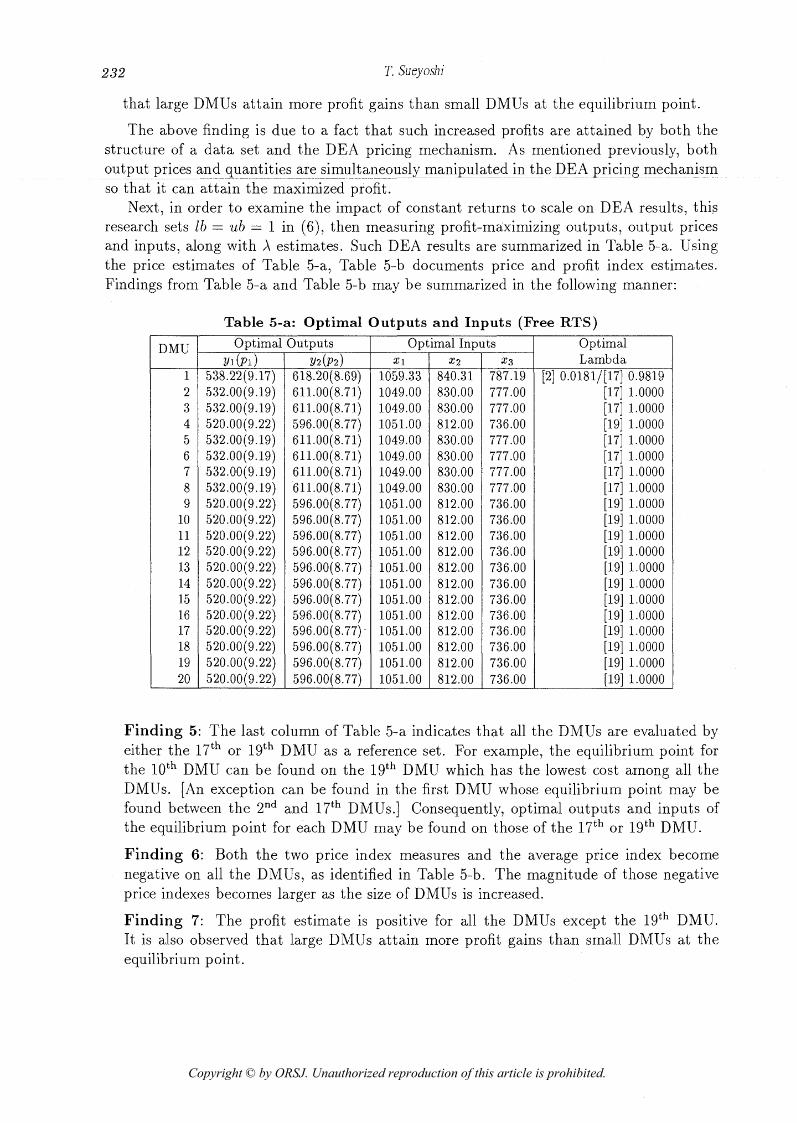
Next, in order to examine the impact of constant returns to scale on DEA results, this research sets lb = ub = 1 in (6), then measuring profit-maximizing outputs, output prices and inputs, along with A estimates. Such DEA results are summarized in Table 5-a. Using the price estimates of Table 5-a, Table 5-b documents price and profit index e~tima~tes. Findings from Table 5-a and Table 5-b may be summarized in the following manner:

Table 5-a: Optimal Outputs and Inputs (Free RTS)

DMU

1 2 3 4 5 6 7 8 9

10 11 12 13 14 15 16 17 18 19 20

Optimal Outputs Y l ( P I ) ~ 2 ( ~ 2 )

Optimal Inputs 7

Optimal Lambda

[2] 0.0181/[17] 0.9819 [l71 1.0000 [l71 1.0000 [l91 1.0000 [l71 1.0000 [l71 1.0000 [l71 1.0000 [l71 1.0000 [l91 1.0000 [l91 1.0000 [l91 1.0000 [l91 1.0000 [l91 1.0000 [l91 1.0000 [l91 1.0000 [l91 1.0000 [l91 1.0000 [l91 1.0000 [l91 1.0000 [l91 1.0000

Finding 5: The last column of Table 5-a indicates that all the DMus are evaluated by either the or lg th DMU as a reference set. For example, the equilibrium point for the loth DMU can be found on the 1gth DMU which has the lowest cost among all the DMUs. [An exception can be found in the first DMU whose equilibrium point may be found between the 2nd and 17th DMUs.] Consequently, optimal outputs and inputs of the equilibrium point for each DMU may be found on those of the or l g t h DMU.

Finding 6: Both the two price index measures and the average price index become negative on all the DMUs, as identified in Table 5-b. The magnitude of those negative price indexes becomes larger as the size of DMus is increased.

Finding 7: The profit estimate is positive for all the DMus except the lg th DMU. It is also observed that large DMus attain more profit gains than small DMus at the equilibrium point.


DEA Pricing System

Table 5-b: Price Index and Profit Index (Free RTS)

DMU

1 2 3 4 5 6 7 8 9

10 11 12 13 14 15 16 17 18 19 2 0

Price Index (1st Output)

(%l -11.29 -11.39

-9.93 -8.34 -9.54

-10.59 -9.27 -8.89 -6.10 -6.47 -2.33 -1.43 -2.56 -2.56 -3.25 -0.88 -0.88 -1.65 -0.66 -1.10

Price Index (2nd Output)

(%l -18.07 -18.18 -15.67 -13.02 -14.76 -16.60 -14.45 -13.56 -9.22 -9.76 -3.06 -3.06 -7.08 -5.16 -2.69 -2.33 -0.69 -1.86 -0.34 -1.04

Average Price Index

(%l -14.68 -14.79 -12.80 -10.68 -12.15 -13.60 -11.86 -11.22 -7.66 -8.11 -2.69 -2.24 -4.82 -3.86 -2.97 -1.60 -0.78 -1.76 -0.50 -1.07

Note: Profit Increase = Optimal Profit

Optimal Profit

1975.76 1913.53 1813.72 1199.42 1547.05 1763.53 1512.73 1393.67 715.98 781.16 446.68 375.12 991.20 750.28 312.63 290.85

19.84 201.01 -55.28 67.61

Profit Increase

856.11 842.60 757.42 810.05 830.85 834.73 822.60 820.21 700.11 718.09 220.39 177.19 24 1.04 235.54 262.47 134.61 67.85

159.94 48.29

104.23

Observed Profit

Profit Index

(%l 56.67 55.97 58.24 32.46 46.29 52.67 45.62 41.15

2.22 8.07

50.66 52.76 75.68 68.61 16.04 53.72

-241.99 20.43

187.36 -54.16

6. Conclusion and Future Extensions This article presents a new type of DEA application to the determination of a profit-based pricing system. A unique feature of this study is that it incorporates important economic concepts (e.g., a demand function, a profit-maximizing price, and a market equilibrium) into the DEA framework. Furthermore, the new DEA approach is reformulated by nonlinear programming and its pricing properties are explored from the Kuhn-Tuker condition. Thus, this article is an initial step to enhance DEA practicality in setting multiple commodity prices. The use of the proposed DEA pricing mechanism is confirmed with an illustrative data set.

There are two future research extensions to be mentioned. First, this article accepts an assumption that we can access an input price vector (W), along with an output price vector (P) which is unknown but computable from an output quantity vector ( V ) in this study. The determination of P on a market equilibrium is the objective of this research and such market equilibrium prices are compared with real prices. Meanwhile, a conventinal use of DEA assumes that it does not depend upon such accessibility to both W and P . It is true that if we can access such information regarding W, we should fully utilize the information. However, in many cases where we cannot obtain such information on W, DEA users can substitute W by DEA dual variables, as explored in Section 2 of this article, using some a priori information such as previous experience and theory. As an important research extension, this article will present another DEA approach for commodity pricing, omitting the need of W. This is a future research task. Another future research may be due to our research requirement, indicating that this study needs to apply the proposed DEA approach to the pricing issues of many commodities in private economics. This is another important future extension of the article. This future research task may be found in theoretical extensions on DEA pricing from the perspective of the general equilibrium


234 T. Sueyoshi

theory intensively investigated in economics. Finally, it is hoped that this article makes a small contribution on the establishment of

the DEA-based price setting system.

Reference Bazarra, M. S. and Shetty, C. M., Nonlinear Programming, John Wiley & Sons, 1979.

Chang, Y. and Sullivan, R. S., QSB (Quantitative Systems for Business Plus), Prentice Hall, 1991.

Charnes, A., Cooper, W. W. and Rhodes, E., "Measuring the Efficiency of Decision Making Units," European Journal of Operational Research, 2 (1978), 429-444.

Debreu, G., Theory of Value, Yale University Press, 1959.

Lemke, C. E., "A Method of Solution for Quadratic Programs", Management Science, 8 (1962), 442-455.

Kaplan, R. S., Advanced Management Accounting, Prentice-Hall, Inc., 1982.

Schrage, L., Linear, Integer and Quadratic Programming with LINDO, The Scientific Press, 1981.

Seiford, L. H., "Data Envelopment Analysis: The Evolution of the State of the Art (1978- 1995)", The Journal of Productivity Analysis, 7 (1996), 99-137.

Shang, J . and Sueyoshi, T. , "A Unified Framework for the Selection of a Flexible Manufac- turing System," European Journal of Operational Research, 85 (1995), 297-315.

Sueyoshi, T., "Estimation of Stochastic Frontier Cost Function Using Data Envelopment Analysis: An Application to the AT&T Divestiture," Journal of the Operational Re- search Society, 42 (1991), 463-477.

Sueyoshi, T., "Measuring Technical, Allocative and Overall Efficiencies using DEA Algo- rithm," Journal of the Operational Research Society, 43 (1992a), 141-155.

Sueyoshi, T., "Measuring Industrial Performance of Chinese Cities by Data Envelopment Analysis," Socio-Economic Planning Sciences, 26 (1992b), 75-88.

Sueyoshi, T., "Algorithmic Strategy for Assurance Region Analysis in DEA," Journal of the Operational Research Society of Japan, 35 (1992c), 62-76.

Sueyoshi, T., "Stochastic Frontier Production Analysis: Measuring Performance of Public Telecommunications in 24 OECD Countries," European Journal of Operational Re- search, 74 (1994), 466-478.

Sueyoshi, T., "Data Envelopment Analysis: Formulations and Economic Interpretation,'' Mathematical Japonica, 42 (1995a), 187-200.

Sueyoshi, T., "Production Analysis in Different Time Periods: An Application of Data Envelopment Analysis," European Journal of Operational Research, 86 (1995b), 216- 230.

Sueyoshi, T., "Ramsey Tariff Structure of NTT Basic Telephone Service: Marginal Cost- Based DEA Application (in Japanese)," Operations Research: Communication of the Operational Research Society of Japan, 40 (1995c), 701-705.

Sueyoshi, T., "Divestiture of Nippon Telegraph & Telephone," Management Science, 42 (1996a), 1326-1351.



Sueyoshi T., "Measuring Scale Efficiencies and Returns to Scale of Nippon Telegraph & Telephone in Production and Cost Analysis," Management Sciencq (Printing, 1996b).

Sueyoshi, T., "Tariff Structure of Japanese Electrical Power Services: Marginal Cost-Based DEA Application," Technical Report of Science University of Tokyo (1996~) .

Tone, K., Data Envelopment Analysis (in Japanese), 1st ed., Nippon Kagaku Gijutsu Ren- mei, Tokyo, 1993.

Toshiyuki Sueyoshi Science University of Tokyo Department of Industrial Administration 2641 Yamazaki, Noda-shi, Chiba 278, Japan


Documents

DEA PRICING SYSTEM