Embed Size (px)
Citation preview
Glasgow Theses Service http://theses.gla.ac.uk/
de Wert, Leoni (2012) Anti-predator adaptations and strategies in the Lepidoptera. PhD thesis http://theses.gla.ac.uk/3541/ Copyright and moral rights for this thesis are retained by the author A copy can be downloaded for personal non-commercial research or study, without prior permission or charge This thesis cannot be reproduced or quoted extensively from without first obtaining permission in writing from the Author The content must not be changed in any way or sold commercially in any format or medium without the formal permission of the Author When referring to this work, full bibliographic details including the author, title, awarding institution and date of the thesis must be given.
Anti-predator adaptations and strategies in the Lepidoptera
Leoni de Wert (MSci)
Submitted in fulfilment of the requirements for the degree of Doctor of Philosophy
Institute of Biodiversity, Animal Health &
Comparative Medicine. College of Medical, Veterinary & Life Sciences.
University of Glasgow
2012
© Leoni de Wert
2
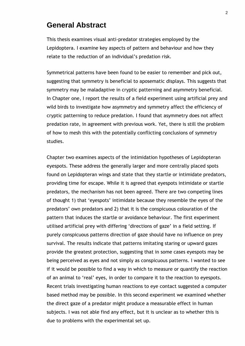
General Abstract
This thesis examines visual anti-predator strategies employed by the
Lepidoptera. I examine key aspects of pattern and behaviour and how they
relate to the reduction of an individual’s predation risk.
Symmetrical patterns have been found to be easier to remember and pick out,
suggesting that symmetry is beneficial to aposematic displays. This suggests that
symmetry may be maladaptive in cryptic patterning and asymmetry beneficial.
In Chapter one, I report the results of a field experiment using artificial prey and
wild birds to investigate how asymmetry and symmetry affect the efficiency of
cryptic patterning to reduce predation. I found that asymmetry does not affect
predation rate, in agreement with previous work. Yet, there is still the problem
of how to mesh this with the potentially conflicting conclusions of symmetry
studies.
Chapter two examines aspects of the intimidation hypotheses of Lepidopteran
eyespots. These address the generally larger and more centrally placed spots
found on Lepidopteran wings and state that they startle or intimidate predators,
providing time for escape. While it is agreed that eyespots intimidate or startle
predators, the mechanism has not been agreed. There are two competing lines
of thought 1) that ‘eyespots’ intimidate because they resemble the eyes of the
predators’ own predators and 2) that it is the conspicuous colouration of the
pattern that induces the startle or avoidance behaviour. The first experiment
utilised artificial prey with differing ‘directions of gaze’ in a field setting. If
purely conspicuous patterns direction of gaze should have no influence on prey
survival. The results indicate that patterns imitating staring or upward gazes
provide the greatest protection, suggesting that in some cases eyespots may be
being perceived as eyes and not simply as conspicuous patterns. I wanted to see
if it would be possible to find a way in which to measure or quantify the reaction
of an animal to ‘real’ eyes, in order to compare it to the reaction to eyespots.
Recent trials investigating human reactions to eye contact suggested a computer
based method may be possible. In this second experiment we examined whether
the direct gaze of a predator might produce a measurable effect in human
subjects. I was not able find any effect, but it is unclear as to whether this is
due to problems with the experimental set up.
3
In Chapter three I investigate a factor often over looked in the study of crypsis,
that of the behavioural adaptations that can enhance its efficiency. The larvae
of the early thorn moth (Selenia dentaria) masquerade as twigs, using both
colouration and behaviour adaptations. I compared the angle at which the larvae
rested, to the angle at which real twigs deviate from the main stem. The results
found that the larvae showed variation in their angle of rest and do not appear
to match the angle of real twigs on the host tree. This result suggests that
perfectly matching the angles of real twigs is not necessary to twig mimicry.
While carrying out this experiment it was noticed that a breeze appeared to
increase larval activity and induced a ‘swaying’ behaviour. This led me to
examine whether mimic species may utilise the visual ‘noise’ produced by windy
conditions to camouflage movement. Firstly, a small ‘proof of concept’ pilot was
carried out, followed by a larger study using 2 different twig mimic species. The
study involved measuring movement and swaying behaviour in 3 conditions (still
air, wind setting 1 and 2). The results suggest that cryptic and mimetic
lepidopteran species may use windy conditions to camouflage their movements
and that some species may employ specialised ‘swaying’ behaviours. Cryptic
species are limited in opportunities to move between foraging sites without
increasing detection by predators, therefore, any adaptation that might reduce
detection is extremely advantageous.
In Chapter four I examine how conspicuousness and colouration are affected by
living in a group, particularly in relation to other group members. A field
experiment using groups of artificial prey, with differing densities and group
sizes was used to explore the effect of group size and density on the predation
risk and detectibility of cryptic prey. My results show that, as expected, larger
groups are more likely to be detected, but that the increase is much slower than
a linear increase. This suggests that groups must increase considerably in size
before any individual group member will suffer increased predation risk.
The second experiment examines the ‘oddity effect’ and how it affects
predation. This hypothesises that when confronted by grouped prey, predators
can increase their kill rate by concentrating their efforts on capturing unusual or
‘odd’ prey, a strategy that reduces the ‘confusion effect’. A field experiment
was conducted with groups composed of differing proportions of two artificial
4
cryptic prey types. Groups with odd individuals did not suffer an increase in
conspicuousness and were not attacked more often. However, once located and
attacked the groups did suffer a greater predation rate. Odd individuals were
predated at a greater rate than normal individuals and the rate did not change
as more or less odd individuals were added to the group. A computer based
‘game’ was used to further investigate the oddity effect. The results from the
initial run of the game appeared to show strong evidence for the oddity effect,
with a further significant increase in this effect when attention is split between
foraging for prey and scanning for predators. To be confident of this result the
experiment was repeated with the ‘odd’ and ‘normal’ seed patterns reversed.
The new data set strongly suggested that much of the effect seen in the previous
experiment was due to a difference in pattern visibility between the two seed
patterns. Nevertheless, the results indicated that selecting odd seeds is quicker
than selecting normal seeds. The results from both the field and computer trials
suggest that preference for odd prey may improve predator foraging speed and
efficiency.
Chapter five investigates whether cryptic and non-defended prey could reduce
their predation risk by grouping with aposematic and defended prey. This was
tested using artificial prey in a field setting. My results show that undefended
non-aposematic prey can benefit by grouping with aposematic prey with no
evidence that predation rates for aposematic prey were adversely affected by
this association. If confirmed this might illuminate the origins of Batesian
mimicry.
I have investigated a range of anti-predator adaptations and strategies in the
Lepidoptera and in particular pattern elements and use of crypsis and
aposematic displays. These anti-predator strategies are important in that they
modify predation rate and so directly influence the evolution of species. While I
have been able to provide evidence for some current hypotheses, in many
respects my results demonstrate that there is still a lot to learn about visual
anti-predatory strategies.
5
Table of Contents
General Abstract ........................................................................... 2 Table of Contents .......................................................................... 5 List of Tables................................................................................ 7 List of Figures ............................................................................... 8 Acknowledgements........................................................................ 10 Author’s Declaration ...................................................................... 12 Introduction ................................................................................ 13 Chapter 1. Importance of asymmetry in the crypsis of model moths.............. 20
1.1.1 Materials and Methods.................................................... 23 1.1.2 Results ...................................................................... 26 1.1.3 Discussion................................................................... 27
Chapter 2. Effectiveness of Lepidopteran Eyespots in deterring predators. ..... 31 2.1 Is apparent direction of gaze important? ................................... 31
2.1.1 Materials & Methods ...................................................... 34 2.1.2 Results ...................................................................... 38 2.1.3 Discussion................................................................... 40
2.2 Does the direct gaze of a predator have any costs to prey? ............. 44 2.2.1 Materials & Methods ...................................................... 45 2.2.2 Results ...................................................................... 48 2.2.3 Discussion................................................................... 50
Chapter 3. Masquerade and cryptic behaviour in Lepidopteran larvae............ 52 3.1 How does resting position influence crypsis? ............................... 52
3.1.1 Materials and Methods.................................................... 55 3.1.2 Results ...................................................................... 58 3.1.3 Discussion................................................................... 60
3.2 Concealing movement. How does movement influence crypsis? ........ 64 3.2.1 Materials & Methods ...................................................... 67 3.2.2 Results ...................................................................... 72 3.2.3 Discussion................................................................... 76
Chapter 4. Effects of grouping and group composition on crypsis. ................ 80 4.1 Does group size or density have an effect on predation rate? ........... 80
4.1.1 Materials & Methods ...................................................... 81 4.1.2 Results ...................................................................... 85 4.1.3 Discussion................................................................... 87
4.2 Field test of the effect of ‘oddity’ within a group on predation risk. .. 90 4.2.1 Materials & Methods ...................................................... 93 4.2.2 Results ...................................................................... 96 4.2.3 Discussion................................................................... 97
4.3 Computer based test of the effect of ‘oddity’ within a group on predation risk. .........................................................................101
4.3.1 Materials & Methods .....................................................102 4.3.2 Analysis ....................................................................106 4.3.3 Results Part 1 .............................................................108 4.3.4 Results Part 2 .............................................................112 4.3.5 Discussion..................................................................115
Chapter 5. Protection by association: Evidence for Aposematic commensalism120 5.1.1 Methods & Materials .....................................................123 5.1.2 Results .....................................................................127 5.1.3 Discussion..................................................................130

6
General Discussion .......................................................................135 Appendix i. Colour and Shadow ........................................................139 Appendix ii. Comparison of Eyespot experimental techniques and methodologies..............................................................................................147 Appendix iii. British Caterpillar Database ............................................151 Supplementary Materials ................................................................152 List of References ........................................................................154
7
List of Tables
Table 2–1. Word list & images used..................................................... 46 Table 2–2. No. of each Image/Word string conditions used......................... 49 Table 3–1. Cross-tabulation - Matching Y(1)/N(0) * 90°/180° ...................... 60 Table 4–1. Probability of group predation over 3 temperature ranges ............ 85 Table 4–2. Group Spread - Probability of Attack...................................... 86 Table 4–3. Number of groups attacked by Group size and spread.................. 86 Table 4–4. Treatment Groups............................................................ 93 Table 4–5. Game parameters (All modifiable parameters).........................103 Table 4–6. Parameters of Pilot Study..................................................103 Table 4–7. Pilot Results..................................................................104 Table 4–8. Full Study Game Parameters ..............................................105 Table 4–9. List & definitions of data collected.......................................105 Table 4–10. Overview of Basic Figures & Results ....................................108 Table 4–11. Average time to pick odd & normal seeds for the first 10 seeds. ..109 Table 4–12. Average proportion of Odd & Normal seeds ...........................110 Table 4–13. Summary of seeds collected in Non-predator games. ................110 Table 4–14. Mean Odd/Normal Seeds in Predator & Non-predator treatments. 111 Table 4–15. Overview of Basic Figures & Results ....................................112 Table 4–16. Average time to pick odd & normal seeds for the first 10 seeds. ..113 Table 4–17. Average proportion of Odd & Normal seeds ...........................114 Table 4–18. Summary of Non-predator games........................................114 Table 4–19. Mean Odd/Normal Seeds in Predator & Non-predator treatments. 115 Table 5–1. Number and type of seed in each treatment Group. ..................123 Table 5–2. Mann-Whitney U Test, P Green & UnP Red seeds. .....................127 Table 5–3. Mann-Whitney U Test, UnP Green & P Red seeds. .....................129 Table 5–4. Mann-Whitney U Test, P Green & Red seeds. ...........................129 Table 5–5. Mann-Whitney U Test, across all experiments. .........................130
8
List of Figures
Figure 1–1. Peach blossom moth (Thyatira batis)..................................... 22 Figure 1–2. Asymmetrical Stimuli (not actual size)................................... 23 Figure 1–3. Asymmetry Stimuli, Cumulative survival probability................... 26 Figure 1–4. Combined Asymmetry Levels, Cumulative survival probability....... 27 Figure 2–1. Examples of two types of Eyespots ....................................... 32 Figure 2–2. Locations of experimental sites ........................................... 34 Figure 2–3. Eyegaze Stimuli (not actual size) ......................................... 35 Figure 2–4. Pollok Country Park - Mountain Bike Tracks ............................. 37 Figure 2–5. Graph depicting the fate of different stimuli types.................... 38 Figure 2–6. Cumulative survival probability ........................................... 39 Figure 2–7. Colour word and neutral signs ............................................. 45 Figure 2–8. Stimuli used in Phase 3 ..................................................... 46 Figure 2–9. Neutral Stimuli............................................................... 47 Figure 2–10. Time course of Phase 3 and example stimuli .......................... 48 Figure 2–11. Average Reaction Time for each Image/String condition with SE .. 49 Figure 3–1. Pacific tree frog (Hyla regilla) - green & brown colour morphs ...... 52 Figure 3–2. Resting positions S. dentaria .............................................. 54 Figure 3–3. Defining resting on 90° and 180° twigs .................................. 56 Figure 3–4. Measuring angle in GIMP 2.6 ............................................... 56 Figure 3–5. Direction of resting postiton............................................... 57 Figure 3–6. Frequency of angles (°)..................................................... 58 Figure 3–7. Angles of larva and Hawthorn (means and variance)................... 59 Figure 3–8. Snowshoe hare (Lepus americanus)....................................... 64 Figure 3–9. Duvaucel's gecko (Hoplodactylus duvaucelii)............................ 64 Figure 3–10. Clamp & twig set up (Image author’s own) ............................ 68 Figure 3–11. Clamp & artificial ‘twig’ set-up for Experiment 1 .................... 70 Figure 3–12. Experiment 2 set up, Enclosed Clamp & dowelling ................... 71 Figure 3–13. Proportion of larvae were scored as ‘swaying’ ........................ 72 Figure 3–14. Proportion of larvae scored as ‘travelling’............................. 73 Figure 3–15. Mean percentage ‘Travelling’ and ‘Swaying’ (S. dentaria) .......... 73 Figure 3–16. Mean percentage ‘Travelling’ and ‘Swaying’ (B. betularia) ......... 74 Figure 4–1. Experiment Site.............................................................. 81 Figure 4–2. Example seed groups........................................................ 82 Figure 4–3. Method for locating seed groups .......................................... 83 Figure 4–4. Group Size - Probability of Attack ........................................ 86 Figure 4–5. Study Site ..................................................................... 93 Figure 4–6. Treatments L-R: Control, Group 1, Group 2, Group 3.................. 94 Figure 4–7. Method for locating seed groups .......................................... 94 Figure 4–8. Percentage of individuals surviving per group .......................... 96 Figure 4–9. Number of Groups that have had at least 1 seed removed............ 97 Figure 4–10. Screen Print of Oddity Game............................................102 Figure 4–11. Seed Ids.....................................................................104 Figure 4–12. L-R: Odd Seed (9), Normal Seed (8). ...................................104 Figure 4–13. L-R: Normal Seed (9), Odd Seed (8). ...................................107 Figure 4–14. Time (in seconds) to pick seeds.........................................109 Figure 6–1. Cryptic patterning and resting position .................................136 Figure 6–2. Butterflies that are both cryptic and aposematic .....................137 Figure 6–3. Reflectance and absorption...............................................140 Figure 6–4. Absorbance spectra of free chlorophyll .................................141 Figure 6–5. Light Spectra. ...............................................................142

9
Figure 6–6. Small Copper (Lycaena phlaeas) .........................................144 Figure 6–7. Shape from Shading. .......................................................145 Figure 6–8. Peach blossom, (Thyatira batis) spots viewed as 'holes' ..............146

10
Acknowledgements
I would like to take time to thank all those who have helped and guided me
during my doctoral study.
Firstly and foremost I want to give me sincerest thanks to my supervisor, Prof.
Graeme Ruxton. His support, patience, perpetual energy and enthusiasm in
research has motivated and inspired many students here at Glasgow University
and I count myself as one of them. He was always accessible and willing to help
me with my research and as a result, research life has been a rewarding and
enjoyable experience.
Thanks also go to Dr. Andrew Higginson and Dr. John Skelhorn who kindly did
their best to answer my questions and emails. Special thanks to Dr Hannah
Rowland who was always happy to give me advice and encouragement. I also
need to thank her along with Dr John Delf and Richard Sutcliffe of the Glasgow
Museums for supplying me with the caterpillars I needed to finish my
experiments. Massive thanks to Patrick Costello, Kevin Mahon and Alison Shand
who became my legs after my knee injury and without whom I could not have
finished my fieldwork.
I also need to say how much I appreciated all the staff of the Graham Kerr
Building without whom the place would quickly descend into chaos! Special
thanks to; our amazing division secretaries Lorna Kennedy and Florence
McGarrity (who always know where you need to go or who you need to speak to);
Jeff Hancock and Maggie Reilly for their advice and help on numerous occasions;
the technical staff John Lawrie, Graham Law, Pat McLaughlin and Alastair Kirk,
who have provided much needed help on more than one project; and of course
our janitors Alan Pringle and George Gow, endlessly cheerful and always happy
to help; and finally to the many cleaners who have patiently cleaned around us
to make sure our office remains a pleasant place to work!
To my wonderful office mates, past and present, you have my unending
gratitude! Your jokes, banter and camaraderie kept me sane and upbeat even
when things weren’t going to plan. To the office ‘mum’ Ashley – you showed me
the ropes and always had good banter, cups of tea and cake. You were always

11
there to help, even when you had more than enough of your own work! I can’t
think of a better person to be teaching the next generation of scientists. To
Katherine – I have to especially thank you for introducing me to Sandy’s art class
in those last stressful months. They provided me with a well needed calm in the
sea of thesis writing. To Vic Paterson-Mackie - your cake and craft ideas
provided another very important (and tasty) distraction from writing up. Not
only have I finished my doctorate, I have gained new crafting skills! To Julissa
Tapia – near the end it was just the two of us and your cheerful smile and chat
were truly appreciated. To all the rest of the GK crew Sarah Al-Ateeqi, Eliza
Leat, Gus Cameron, Donald Reid, Emma Louise Lowe, Shaun Killen, Zara
Gladman and Gemma Jennings - thanks for all the chat, lunchtime clockword,
Skeptics and other random beer, cheese and cake related activities!
To my best friends Morna Fell, Aimee McMorrow, Naomi Spirit-Hawthorn and my
sister Nicole de Wert-Wightman. Thanks for putting up with me disappearing for
weeks on end when things were busy. Our regular ‘Ladies lunches’ and playing
with the babies was a welcome (if sometimes exhausting) change from research.
To my parents, who were always there with encouragement and support when I
needed it, I am eternally grateful. Without your support and advice, especially
after I tore my ACL, finishing would have been a far harder task. Thanks also to
my parents-in-law Marlene and Alexander Anderson for helping out so much
when I was on crutches and for the all important proof-reading. We wouldn’t
have managed without all your help and support.
Finally, to my wonderful husband David. Thank you for being my support and
strength. For putting up with the stress, tears and general oddness! On top of
your own work you had to look after me and our 3 cats through 2 knee
operations and almost 5 months of me hobbling around on crutches. I don’t know
how you did it, but I’m very glad you did. x

12
Author’s Declaration
I declare that the work recorded in this thesis is entirely my own and is of my
own composition. Patrick Costello and Alison Shand aided with data collection
for Chapter 1, Patrick Costello aided in collecting data for chapter 2 (Section
2.1) and Kevin Mahon aided with data collection for chapter 5. No part of this
thesis has been submitted for another degree.
Chapter 5 is to be published in the Biological Journal of the Linnean Society,
2012.

13
Introduction
No organism (from the smallest bacterial cell to the blue whale) lives or acts in
isolation. We interact with a host of other species every hour of every day and,
along with the physical environment, it is the sum of those interactions that acts
to shape life on Earth. We can broadly characterise these interactions into three
categories. The first and arguably the most widespread, since all organisms
experience it to some degree, is that of competition. Competition can occur as
both an inter-species and intra-species effect, and is where individuals compete
for a share of a limited resource. That resource can be anything from space
within a habitat, to food or a mate. Those organisms that compete successfully
are the most likely to survive and pass on their genetic information to the next
generation, making competition a vital component of evolutionary change.
Secondly there are those interactions that involve two or more species, where
the relationship benefits one or more of those species. Where only one party
benefits, but the other suffers no effect (positive or negative) the relationship is
described as commensalism and where all parties benefit from the relationship it
is termed mutualism. In some instances these relationships are obligatory, but
this is not always so.
Finally, there are those interactions in which one party is exploited or eaten by
another. These parasite-host and predator-prey interactions are characterised by
the dichotomy of the costs and benefits, with the negative effects all resting on
the host/prey end of the equation. A very simple food chain will have plants at
its base which are fed on by organism A, which is predated on by organism B,
which in turn is predated on by organism C, but it is very rare that such a simple
food chain is found in the natural world. More often organisms are part of a
larger food web, with each organism being party to multiple interactions,
feeding on and being predated on by multiple other species.
In such complex communities there is often intense competition between
predators for the various prey species. That competition ensures that only those
predators that are able to find and capture prey the most efficiently are the
most likely to survive to pass on their genes. This ensures that any adaptation or
specialisation that increases a predator’s ability to hunt and capture prey is
Introduction 14
maintained within the population. This selection for ever greater efficiency has
led some predators to evolve specialised adaptations to hunt one particular prey
type. For instance the aye-aye (Daubentonia madagascariensis) has a highly
specialised long, thin, third digit which is not used during locomotion, but is
used almost exclusively in the extraction of grubs from tree trunks (Lhota et al.,
2008) or the peregrine falcon (Falco peregrinus) that can accelerate to speeds
well in excess of 300km/h when diving to strike its prey (Baumgart, 2011). Yet,
still there are some grubs that are able to escape the aye-aye’s sensitive probing
finger and some birds that are able to evade the peregrine falcon’s dive, and
those individuals are the ones that are most likely to contribute their genes to
the next generation. This is the so often mentioned ‘evolutionary arms race’,
with prey evolving more elaborate and diverse defences against their predators
and predators evolving new mechanisms to combat them. This dynamic between
predator and prey is an important and powerful evolutionary force, leading to
adaptations on both sides of the predator-prey relationship constantly shifting
and changing over evolutionary time. However, while we understand the
importance of the predator-prey relationship we still do not understand many of
the intricacies of how certain defensive or predatory mechanisms work or what
steps led to their development. To fully understand these we need to ask very
specific questions about the mechanisms involved, and one of the best ways to
answer those questions is through field and laboratory experiments using real
organisms. To do this we need to select our study organism carefully.
The ubiquitous nature of the Lepidoptera has led them to be intensively studied,
beginning with the earliest naturalists and biologists. The anatomy and the
morphology of both the immature and adult stages have been extensively
studied and due to their availability are often used as experimental subjects for
anatomy and physiology studies (Ed. Capinera, 2008). The Lepidoptera are also
of interest in ecological studies, where the segregation of habitat, dietary
requirements and morphology between life stages has provided fertile ground for
study. They also make an effective ‘prey’ organism in studies investigating
predator-prey interactions as they are preyed upon by a wide variety of
organisms, from insects and arachnids to mammals and birds, which between
them have a diverse range of hunting techniques. For example avian predators
are predominantly visual predators and so most are well equipped to hunt using
Introduction 15
sight with sensitive tetrachromatic colour vision to search out and target prey
(Finger and Burkhardt, 1994). Therefore the most effective anti-predator
adaptations a Lepidopteran will have against avian attack is likely to be visual.
Predators that use sight to hunt are known to use shape, colour and pattern to
form search images to increase foraging efficiency (Pietrewicz and Kamil, 1979).
However, there are also a number of ways that colouration and pattern can be
utilised by prey organisms to reduce their chances of being predated. These fall
into three broad categories; those that reduce predation by avoiding detection
entirely by predators, by being detected but advertising their unsuitability as
prey (Ruxton et al., 2004) and by being detected but misclassified as something
non-edible (Skelhorn et al., 2010b). All three strategies described are found
within the Lepidoptera and in some cases a single species may use different
strategies at different points within their lifecycle(Gamberale and Tullberg,
1996).
The first group describes any type of crypsis or camouflage. In its simplest form
crypsis can take the form of background matching: this is where an organism’s
colouration matches the background colouration of its habitat. An example of
this is the white fur of the arctic fox (Vulpes lagopus) in winter, which blends in
its snowy habitat. This basic type of crypsis can be further enhanced by adding
countershading and/or disruptive patterning. Countershading, where the ventral
surface of an organism is a lighter colour than the rest of the body, is an
extremely common feature of animal colouration (Ruxton et al., 2004).
Disruptive patterning is a pattern that breaks up the body outline and often
includes pattern elements than appear to run over the true body edge or create
false body outlines (Stevens and Merilaita, 2009). Both countershading and
disruptive patterning hinder a predator’s ability to detect or recognise an
organism by disguising the organism’s true outline and have been found to
enhance crypsis and reduce predation by avian predators (Fraser et al., 2007;
Rowland et al., 2007; Stevens and Merilaita, 2009).
The next two groups both assume that the predator will detect the organism but
that it will choose not to attack. The first is arguably another, more complex,
form of crypsis. In this case the prey’s colouration or patterning is used to
mimic the appearance of an inedible model such as a pebble, twig or bird
Introduction 16
faeces. This type of cryptic patterning is called ‘Masquerade’ and when
successful causes predators to misidentify as the prey as its inedible model and
disregarded them (Skelhorn et al., 2010b). This effectively allows the prey
animal to ‘hide’ in plain sight.
Finally we have the use of aposematic or warning colouration. Unlike the
previous types of colouration and patterning, aposematic patterning does not
hide or disguise the prey animal at all. In fact, it does quite the opposite using
conspicuous behaviour, odour, sound or colouration (e.g. red, yellow, black or
orange) to announce unprofitability (usually due to toxicity or distastefulness)
(Cott, 1940; Poulton, 1890). Aposematic displays are generally very conspicuous,
a trait which is thought to 1) enable predators to easily distinguish defended
prey from undefended prey and 2) impose costs that only defended prey can
afford, such as increased detection rates (Sherratt and Beatty, 2003). In some
cases organisms will use a combination of conspicuous signals to startle and
deflect predators. For example the peacock butterfly (Inachis io) hibernates as
an adult with their wings closed hiding their large conspicuous wing spots.
However, if disturbed they flick their wings open and closed several times,
flashing the spots and making a hissing noise (Blest, 1957; Wiklund et al., 2008).
Effective aposematic signalling provides great advantages for survival, but
secondary defences such as toxins can be costly to produce. So why go to the
expense of developing secondary defences yourself when, by mimicking
characteristic patterns and behaviours of those that do, you can benefit without
them? It is not even completely necessary for mimics to perfectly match all
aspects of the model’s patterning, with even imperfect mimicry providing some
protection (Kikuchi and Pfennig, 2010). This type of mimicry is called Batesian
mimicry. A commonly used example of this is the relationship between some
colubrid snakes of the Pliocerus genus (non-venomous and rear-fanged) and the
Miccrurus coral snakes (venomous and front fanged) that live in many of the
same areas of Central America. Where they do co-habitat it has been found that
the patterning of the non-venomous colubrid snakes more closely resembles
their venomous model the coral snake (Greene and McDiarmid, 1981). However,
dishonest signals like those of Batesian mimics can change the effectiveness of
the warning signal. It has been shown that as the ratio of mimics to models
Introduction 17
increases, the effectiveness of the warning signal is reduced and predation rates
for both groups increase (Ruxton et al., 2004).
Conversely, when two or more unpalatable or defended prey species share
similar characteristics and/or patterning it can benefit both species by
strengthening a predator’s association between that pattern and
unprofitability(Mallet and Barton, 1989). This type of mimicry where all parties
are generating an honest signal of secondary defences is called Müllerian
mimicry, and its most celebrated example is that of the Heliconius butterflies of
South America. Here we find groups of heliconiine species, together with some
species from other lepidopteran groups, which all resemble one another in some
way (Brower, 1996).
As we can see, colour and patterning are important factors in determining
predation rates. However, how well these strategies work can also be affected
by whether an organism lives singly or as part of a larger group. Being part of a
larger group has a number of benefits, with the presence of the other group
members diluting the predation risk and making it difficult for predators to
either pick out an individual from the group or approach unseen(Krause and
Ruxton, 2002). However, a large group is unlikely to be able to remain as cryptic
as a single animal. In fact, there is a trade off between the dilution of risk and
increased conspicuousness, with increasing group size easing detection by
predators (Jackson et al., 2005).
Despite all we do know about predator-prey interactions there is still much to be
answered. Through a series of lab and field experiments I have attempted to
look at some of the outstanding questions. There is still much discussion over
asymmetry and its affect in cryptic patterning. In Chapter 1 I report on the
results of a field experiment examining whether asymmetry can enhance cryptic
patterning. To do this I used artificial baits of varying levels of asymmetry and
monitored the predations, with the view that any benefit of asymmetry should
be seen in an increased survival rate for those baits. From there I wanted to look
at one of the most common symmetrical pattern elements found in Lepidopteran
aposematic displays; the eyespot. How eyespots are interpreted by predators is
an important question still being discussed today and in chapter 2 I report on
two experiments I conducted in an attempt to provide evidence to answer this
Introduction 18
question. If eyespots are being interpreted as eyes we might expect that
changing the apparent direction of the ‘eyes’ might have an effect on their
ability to reduce predation rates. With this in mind I conducted an experiment
using artificial baits with the central circle of the ‘eyespot’ off centre so as to
appear to be gazing in different directions. In experiments with humans it has
been found the direct gaze of another person is automatically processed by the
brain. Therefore for my second experiment I wanted to examine if the direct
gaze of another species is able to elicit a similar response and whether there is
any difference made between the binocular gaze of a predatory species to that
of a prey species. To do this a computer trials were designed using the Stroop
test as a basis for measuring attention and reaction times. If a measurable
response was found this may lead to a way of determining if eyespots are being
reacted to in a similar manner to real eyes.
There are often behavioural adaptations that enhance aposematic displays, such
as the startling flashing of eyespots utilised by some Lepidopteran species.
However, comparatively little has been done to examine behavioural equivalents
that enhance camouflage. In Chapter 3 I look at how behaviour is used to
enhance masquerade in two Lepidopteran species with twig mimic larvae. I test
early thorn (Selenia dentaria) to assess whether they adapt their resting position
to better match their food plant. The results from this experiment may go
towards understanding how ‘perfect’ mimicry must be in order to effectively
reduce predation risk. I then used both early thorn (Selenia dentaria) and
peppered moth (Biston betularia) larvae to assess whether they are able to use
behavioural adaptations to camouflage their movement. The ability to move
between habitats or find new food resources without increasing predation risk
would represent a considerable benefit for species that must otherwise remain
still to maintain their masquerade defence.
In Chapter 4 I wanted to examine the effect of group composition on predation.
How does group, size, density and composition of your group affect your chances
of predation? Further does being different from the majority of your group
affect, both your own chance of being predated, and the predation rate for the
group as a whole? Could I find any evidence for the Oddity Effect? To investigate
this I designed field experiments using groups of sunflower seeds with
compositions designed to mimic these scenarios. These were set out and the
Introduction 19
local wild bird population was allowed to remove seeds at will for a set period of
time. In this way I was able to compare predation rates between the different
group types. I then wanted to examine if dividing attention between prey
selection and scanning for predators could change the way the Oddity Effect was
felt. To do this a computer game was designed so that I could use human
volunteers to act as predators and allow for more parameters to be measured
than was possible in the field experiments. Finally, in Chapter 5 I investigate the
effects of associating or grouping with aposematic species when using crypsis.
Here again sunflower seed groups were used as baits, with some baits made
aposematic with additives to change the colour and make the baits distasteful.
Chapter 1 20
Chapter 1. Importance of asymmetry in the crypsis of model moths.
Symmetry is found throughout the animal kingdom in the body plans of almost
all multi-cellular life, from the bilateral symmetry we can see in ourselves to the
radial symmetry found in the phyla Cnidaria and Echinoderamata. It is often
thought that developmental instabilities caused by stress can be seen in the
adult animal in the form of asymmetrical development of patterns and/or form,
making symmetry an honest and potentially important signal of individual quality
(Ciuti and Apollonio, 2011). The effect of symmetry on camouflage or warning
patterns has also been explored using a diverse range of subjects such as
pigeons(Delius and Nowak, 1982), humans (Attneave, 1954) and honey bees
(Horridge, 1996). These studies have shown that patterns that include lines of
symmetry are more easily detected, learnt and reproduced than those with
asymmetry. Consequently symmetry & asymmetry are of interest as pattern
elements in the study of crypsis and aposematism.
Aposematic patterns are conspicuous warning displays intended to advertise
unpalatability and deter predators (Ruxton et al., 2004) Therefore, any pattern
element that may make them more easily identified, recognised and/or
memorised should increase effectiveness. A number of studies have examined
the effect of symmetrical pattern elements in aposematic displays, but with
differing results. Forsman & Merilaita (1999) were able to show that domestic
chicks (Gallus gallus domesticus) were able to learn to avoid unpalatable
artificial prey faster when the pattern consisted of 2 spots of equal size than
when the pattern was asymmetrical in spot size. In a later study (Forsman and
Herrstrom, 2004) it was also shown that symmetry in shape, pattern and colour
enhanced the innate avoidance behaviour of chicks to conspicuous palatable
prey. These results suggested that conspicuous prey would be under strong
selection pressure to maintain symmetrical signals, as they increase innate
avoidance and the rate of aversion learning by predators, both of which have
strong fitness benefits.
However, since publication it has been suggested that the way in which the size
of the stimuli asymmetries & spot areas were calculated in Forsman and
Herstrom’s (2004) study may have confounded overall size differences with
Chapter 1 21
asymmetry differences. This meant that the threshold for discrimination
between symmetrical and asymmetrical stimuli by the birds was in fact between
20% & 32% (Swaddle and Johnson, 2007) rather than around 7.5% as reported.
Also when recalculated it was found that the asymmetrical stimuli used in the
size asymmetry trials had a spot area which was on average 7% smaller than the
symmetrical stimuli (Swaddle and Johnson, 2007) and as other studies have
indicated that conspicuous wing spots are more effective with increased size
(Stevens et al., 2008a) this makes it difficult to determine that differences were
caused by asymmetry alone.
Both of the previous studies mentioned were lab based with the Forsman &
Merilaita (1999) study allowing chicks to select prey from a large number of
artificial stimuli & Forsman & Herstrom’s (2004) study using a 2-way forced
choice design. Even taking in to account some of the possible problems with
Forsman & Herstrom’s study they provide some evidence that symmetry speeds
learning of patterns and that asymmetry in colour and shape increases
predation.
However, a later field study conducted by Stevens et al. (2009b) found that
there was no benefit to symmetry, with asymmetry in shape, size and position
conferring no extra survival cost. The reasons for the difference in results are
uncertain, although it may be that the design of the lab studies and in
particular, the 2-way forced choice test, may not provide results representative
of the decision making processes used by avian predators in the wild, who will
often encounter prey sequentially and make decisions to accept or reject, rather
than decisions about choosing one of two alternatives to accept.
Crypsis, unlike the aposematic patterning we describe above, is used to reduce
detection by matching the colours, patterning and texture of the background an
organism is sitting against(Ruxton et al., 2004). Predators which use vision to
locate cryptic prey must rely on noticing subtle differences in colour, shade,
pattern or texture between their prey and the background(Endler, 1978; Ruxton
et al., 2004). As very few natural substrates or backgrounds contain the type of
bilateral plane of symmetry typical of most animals, symmetry is though to be a
strong visual cue to their presence. In field experiments using artificial moth-
like stimuli, Cuthill et al. (2006a; 2006b) found that symmetry reduced the
Chapter 1 22
effectiveness of both disruptive and back-ground matching patterns with
symmetry incurring a significant fitness cost.
However, as the previous investigations into this phenomenon have used entirely
artificial patterns, we propose to use the patterning of the moth species the
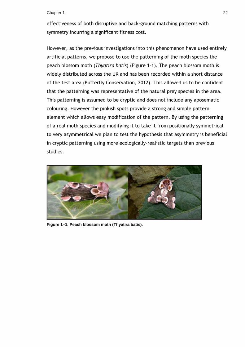
peach blossom moth (Thyatira batis) (Figure 1–1). The peach blossom moth is
widely distributed across the UK and has been recorded within a short distance
of the test area (Butterfly Conservation, 2012). This allowed us to be confident
that the patterning was representative of the natural prey species in the area.
This patterning is assumed to be cryptic and does not include any aposematic
colouring. However the pinkish spots provide a strong and simple pattern
element which allows easy modification of the pattern. By using the patterning
of a real moth species and modifying it to take it from positionally symmetrical
to very asymmetrical we plan to test the hypothesis that asymmetry is beneficial
in cryptic patterning using more ecologically-realistic targets than previous
studies.
Figure 1–1. Peach blossom moth ( Thyatira batis).
Chapter 1 23
1.1.1 Materials and Methods
This experiment was conducted over two seasons and at 3 sites. The first season
between 25th May & 30th Sept 2010 used mixed deciduous woodland at
Dawsholm Park, Glasgow (55°89'61.75"N, 4°31'59.98"W). The second season
between April 26th and July 23rd 2011 used two smaller sites, with the first at the
Glasgow Botanic Gardens, Glasgow, UK (55°52'53.57"N, 4°17'28.02"W) and the
other at Kelvingrove Park, Glasgow, UK (55°52'24.92"N, 4°16'49.50"W). In both
seasons different trees and trials were used to ensure that the same areas were
not used for consecutive trials. For the second season the two sites were used
alternately to ensure that each site was free from the artificial stimuli for a
minimum of 72 hours prior to Day 1 of any run.
Artificial baits were made using modified images of the Peach Blossom moth
(Thyatira batis). The baits were designed with 3 levels of asymmetry plus
controls of symmetrical baits with and without spots. There were 8 treatments
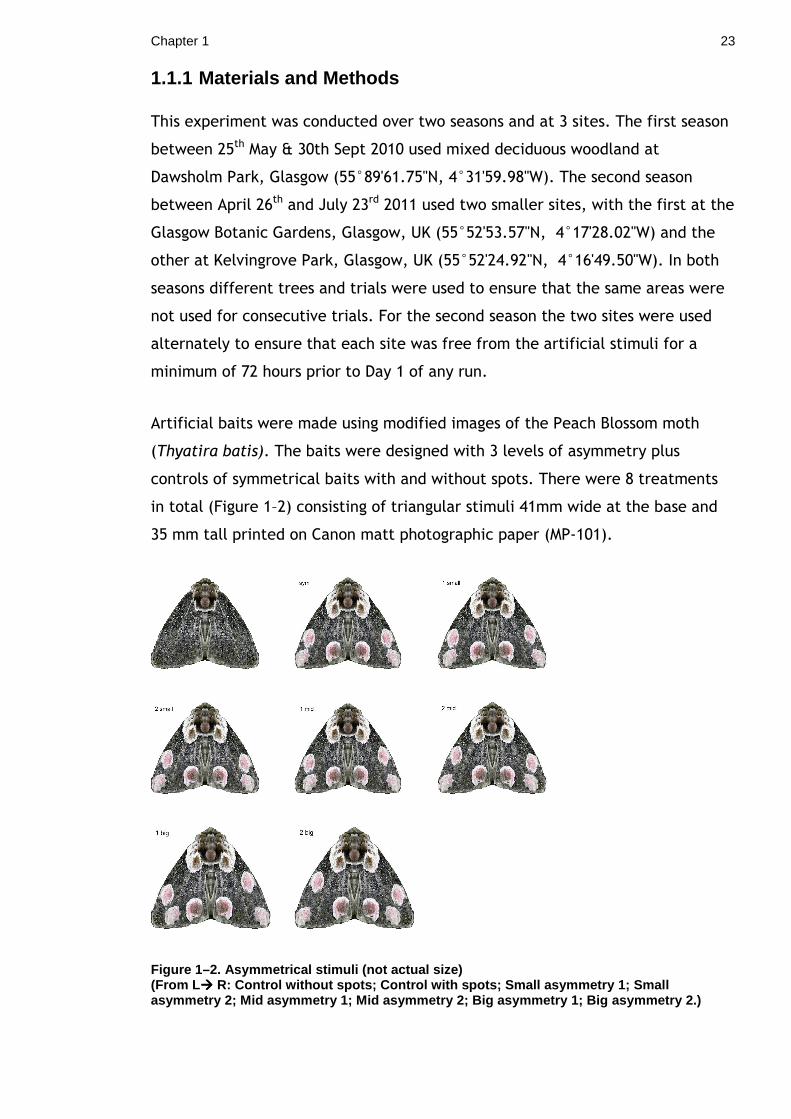
in total (Figure 1–2) consisting of triangular stimuli 41mm wide at the base and
35 mm tall printed on Canon matt photographic paper (MP-101).
Figure 1–2. Asymmetrical stimuli (not actual size) (From L ���� R: Control without spots; Control with spots; Smal l asymmetry 1; Small asymmetry 2; Mid asymmetry 1; Mid asymmetry 2; Big asymmetry 1; Big asymmetry 2.)

Chapter 1 24
Of the 8 stimuli, 2 were designed to act as controls, both with fully symmetrical
designs but one with spots and one without. This enabled us to control for any
effect of the spots and allowed us to compare the effect of symmetry with the
asymmetrical treatments. The 6 remaining stimuli were the treatment groups
with 3 levels of asymmetry. Each pair of stimuli had one which had the
asymmetrical element on the left and another on the right, which allowed us to
control for laterality. This is important as many species show lateralisation and a
preference for one side over another ((Magat and Brown, 2009)). To give a
measure of the relative levels of asymmetry we measured the distance between
the centres of the 2 spots on the outside edges of each stimulus and calculated
the percentage difference between the two sides. The small asymmetry stimuli
were found to be 80% asymmetrical, the medium stimuli are 150% asymmetrical
and the large stimuli 175% asymmetrical, all of which are well above the levels
of asymmetry known to be detectable (Swaddle and Johnson, 2007). With these
stimuli we hoped to be able to discern whether there was any effect of
asymmetry and the degree of asymmetry needed.
The edible component of each bait consisted of a mealworm (frozen overnight,
then thawed) pinned vertically to the centre of the underside of each stimuli.
The mealworm is pinned to the underside with only the tip projecting, rather
than on the surface, as it is important that there is no other source of
asymmetry other than the printed pattern.
On each of 14 days 72 trees (i.e. 9 replicates of each of the 8 baits) were
selected at random with a minimum gap of 10m between them. Only trees
without lichen covering the trunk and that were of at least 0.9m in
circumference were selected. Different sections of the wood were used in
rotation with the same sections of woodland not used in consecutive trials and
care taken to ensure that no tree was used more than once. Stimuli were
assigned randomly to a tree and attached a minimum of 1.5m up from the base
using dressmaker’s pins. Randomisation of the allocations was achieved by
assigning the stimuli to tree using a random number generated by the Excel
function RAND() and using the SORT function to put them in ascending order to
be placed on trees 1-72.
Chapter 1 25
The experiment was conducted over 48hrs with the baits put out on the morning
of day 1 and checked for survival at 2, 4, 24 and 48hrs. Avian predation was
taken to be indicated by complete or almost complete disappearance of the
mealworm. Non-avian predators such as slugs were indicated by the slime trails
left behind and spiders and harvestmen by the mealworms being hollowed out
leaving the empty exoskeleton. While the treatment groups were not watched a
number of different bird species were observed close to or in the immediate
area including blackbirds (Turdus merula), bluetits (Cyanistes caeruleus),
bullfinch (Pyrrhula pyrrhula), carrion crow (Corvus corone), house sparrows
(Passer domesticus), magpie (Pica pica), robin (Erithacus rubecula), rock pigeon
(Columba livia), starling (Sturnus vulgaris) and wood pigeon (Columba
palumbus). Every time the site was visited the date & time of arrival and
departure was noted. Weather conditions and temperature at 9am, 12pm and
5pm were taken from the Met Office website for each day of the experiment.
The collected data was analysed in SPSS and a Cox proportional hazards
regression used to accommodate the censored data and the varying predation
risk throughout the day (Cox, 1972; Klein J.P. & Moeschberger, 2003; Lawless,
2002). Effect sizes are given by the odds ratio (Exp(B)), which is the ratio of the
probability of predation in one treatment compared to the probability of
predation in another treatment. We compared all treatments to the symmetrical
control, so that the Exp (B) values given are the likelihood of predation when
compared with this treatment.
The data were analysed at both the individual stimuli level (8 treatments) and
with the stimuli grouped so that the mirrored stimuli from each asymmetry
grading (small, medium & large) were analysed together giving 5 treatment
groups.
Chapter 1 26
1.1.2 Results
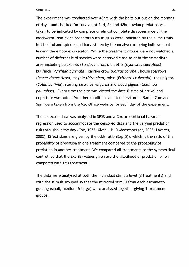
In total we had 23.6% of our stimuli predated by birds and 76.4% censored
stimuli (not eaten by birds), with the majority of stimuli taken within the first
24hrs after placement. None of the stimuli types differed significantly in survival
rate from the symmetrical control (Control/No spots, Wald statistic (WS) =
0.178, p = 0.67, Exp (B) = 1.04; 1S, WS = 2.26, p = 0.13, Exp (B) = 0.86; 2S, WS =
2.95, p = 0.09 Exp (B) = 1.17; 1M, WS = 0.84, p = 0.36, Exp (B) = 0.92; 2M, WS =
0.59, p = 0.44, Exp (B) = 0.93; 1B, WS = 0.36, p = 0.85, Exp (B) = 1.02; 2B, WS =
0.39, p = 0.53, Exp (B) = 0.94). The survival rates for all the stimuli are for the
most part tightly grouped, with no obvious pattern of difference between the
symmetrical and asymmetrical stimuli (Figure 1–3).
Figure 1–3. Asymmetry stimuli, cumulative survival probability - for the 8 stimuli types surviving avian predation over time.
Chapter 1 27
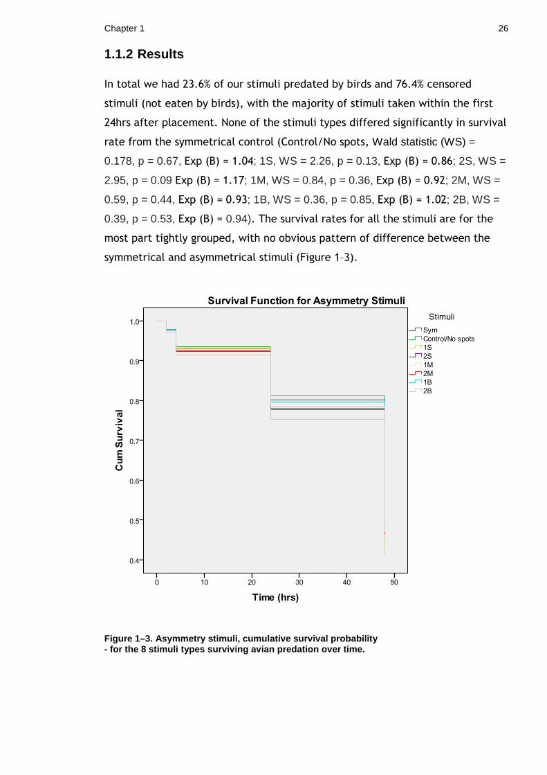
Figure 1–4. Combined asymmetry levels, cumulative s urvival probability - for the 2 control and 3 levels of asymmetry stimu li surviving avian predation over time.
When the stimuli were grouped by the extent of the asymmetry they show
(small, medium & large asymmetry) no significant difference was found between
the different levels of asymmetry (Control/No spots, Wald Statistic (WS) = 0.72,
p = 0.4, Exp (B) = 1.07; Small asymmetry, WS = 1.87, p = 0.17, Exp (B) = 0.89;
Medium asymmetry, WS = 1.14, p = .29, Exp (B) = 1.07; Large asymmetry, WS =
.001, p = .97, Exp (B) = 1.00) (Figure 1–4). Therefore, we conclude that there is
no effect of stimulus type on survival probability to the end of the 48 hour test
period.
1.1.3 Discussion
Our analysis found no significant difference in survival rate between any of the
treatment types. To increase our power to find even a weak effect we combined
data from the asymmetry pairs e.g. small 1 & 2 were combined in to one
treatment. Here, again, we found no significant difference between the stimuli
and again no clear trend or pattern can be seen in the graphed results. From
these results it appears as though asymmetry of wing pattern has no effect on
Chapter 1 28
the survival rate of the stimuli we used. However, we should also point out that
we had a much lower avian predation rate than those reported in some earlier
studies. In Stevens et al’s 2009 paper they described censored (number of
stimuli not taken by birds) rates of 27% and 17.3% which are considerably smaller
than the 76.4% we had.
There are a number of possibilities that might help explain this. It may in part
be due to longer trial durations used in some of the previous studies, with
Stevens et al. conducting trials over 48hrs (2008a), 72 hrs (2009a; 2009b) and 96
hrs (2009b). However, we would argue that by extending the duration of the
trials to achieve a greater predation ratio we risk losing a degree of realism. We
may have been harsher in our judgment of whether a stimulus had been
predated by ‘other’ predators and so censored a larger percentage of the
stimulus.
There may also have been a problem with identifying which predator was
responsible for bait being removed. On a number of our planned checks we
observed the common wasp (Vespula vulgaris) cutting up and removing the
mealworm baits. Since both in this and previous field studies the complete or
almost complete removal of the mealworm bait was used as a signifier of avian
predation, this behaviour by the wasps made determining whether a bait has
truly been removed by a bird extremely difficult. However, as wasps are likely
to locate prey by scent rather than by vision and should not be influenced by the
pattern on the stimuli, as long as the placement of the stimuli and baits is
sufficiently randomized, wasps may increase the average number of baits
removed, but should not affect the overall outcome. This added noise would
make detection of visually-mediated choices by avian predators more difficult to
detect. We suggest that future fieldwork using these techniques should be
carried out during the winter months when wasps are dormant, which would
allow us to be confident that this potentially confounding factor had been
removed.
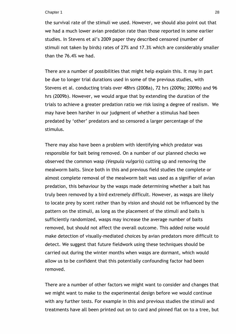
There are a number of other factors we might want to consider and changes that
we might want to make to the experimental design before we would continue
with any further tests. For example in this and previous studies the stimuli and
treatments have all been printed out on to card and pinned flat on to a tree, but
Chapter 1 29
for the majority of moth and butterfly species the naturally adopted resting
position is not flat against the substrate. This may be important as the angle at
which a pattern is viewed will change how much of the pattern as a whole is
seen and its symmetry. Perhaps by using a more 3 dimensional stimuli and bait it
would be possible to more accurately mimic the natural conditions in which the
patterns would be encountered. This may also change the way our stimuli are
seen, as there is a chance that by presenting our stimuli flat we have
inadvertently created paired eyespots where in a more natural position only one
of the spots would be visible at any time (Appendix i for further discussion). It
has been argued previously that only large levels of asymmetry benefit
camouflage and that the developmental changes and sizable mutations this
would require are statistically unlikely (Dawkins, 1976, 1996), however what we
have described above may be a way to work around these constraints.
This raises a couple of possibilities; the first is that if when in a natural resting
position the peach blossom moth only has one wing fully visible at any time, its
patterning will always be asymmetrical; the second is that it maybe that the
pattern can act as either aposematic when viewed directly from above and the
paired symmetrical ‘eyespots’ are visible or cryptic when viewed from any other
angle where only one spot is visible and the pattern is asymmetrical.
We chose, in this instance, to test our hypothesis in a field rather than lab
setting as this adds a degree of realism to the setting that we could not replicate
in the lab. However, there are several problems with this approach that limit
how we can interpret that data. The stimuli we used are not ‘real’ moths and so
we can not be sure that the birds interacting with them as they would a real
moth. It would be interesting to test this possibility with a laboratory study
perhaps with birds only able to approach a 3-dimensional stimulus from either
the side or head on and comparing their willingness to feed.
A potential middle ground between the lab and field studies would be an aviary
study using wild caught birds. An aviary would allow us greater control over the
environment, while still retaining some of the realism of a field experiment. We
would be better able to exclude non-avian predators and be certain that any
bait taken was indeed removed by a bird. We would also be able to observe a
Chapter 1 30
bird’s behaviour before removing the bait, do they observe the bait from a
distance first and from what angle do they approach?
In conclusion, our study found no effect of asymmetry on predation rates, but
there is much that can be done to examine this further. Our results agree with
those recent studies that have found no survival advantage of symmetrical over
asymmetrical markings, so it may be that response to symmetry is something
that only occurs in the simplified visual domain of laboratory test arenas. As
pattern symmetry is widespread throughout the animal kingdom the most
parsimonious explanation might be that, rather than having functional
importance in signalling, symmetry reflects underlying developmental or genetic
constraints.
Chapter 2 31
Chapter 2. Effectiveness of Lepidopteran Eyespots in deterring predators.
2.1 Is apparent direction of gaze important?
It is well known that prey organisms use a variety of patterns and markings to
reduce their risk of predation. These markings can take the form of camouflage,
mimicry and/or conspicuous warning colours(Cott, 1940; Ruxton et al., 2004). A
pattern which has produced quite considerable interest and debate is that of
paired circular ‘eyespots’ most commonly found on tropical fish and
lepidopteran species. Until recently these markings have not been well defined
within the literature and so for the purposes of this report we will use the
definition given by Stevens in his 2005 review.
“… approximately circular marking on the body of an animal, composed of colours contrasting
with the surrounding body area, often comprised of concentric rings and occurring in bilaterally
symmetrically pairs.” (Stevens, 2005)
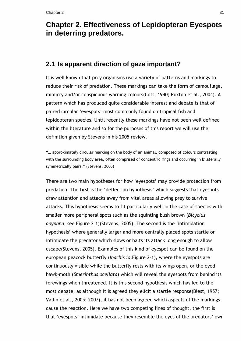
There are two main hypotheses for how ‘eyespots’ may provide protection from
predation. The first is the ‘deflection hypothesis’ which suggests that eyespots
draw attention and attacks away from vital areas allowing prey to survive
attacks. This hypothesis seems to fit particularly well in the case of species with
smaller more peripheral spots such as the squinting bush brown (Bicyclus
anynana, see Figure 2–1)(Stevens, 2005). The second is the ‘intimidation
hypothesis’ where generally larger and more centrally placed spots startle or
intimidate the predator which slows or halts its attack long enough to allow
escape(Stevens, 2005). Examples of this kind of eyespot can be found on the
european peacock butterfly (Inachis io,Figure 2–1), where the eyespots are
continuously visible while the butterfly rests with its wings open, or the eyed
hawk-moth (Smerinthus ocellata) which will reveal the eyespots from behind its
forewings when threatened. It is this second hypothesis which has led to the
most debate; as although it is agreed they elicit a startle response(Blest, 1957;
Vallin et al., 2005; 2007), it has not been agreed which aspects of the markings
cause the reaction. Here we have two competing lines of thought, the first is
that ‘eyespots’ intimidate because they resemble the eyes of the predators’ own
Chapter 2 32
predators and the second stating that it is the conspicuous colouration which
induces the startle or avoidance behaviour. In this second interpretation the
patterns are intimidating simply by being novel (Coppinger, 1969, 1970; Marples
and Kelly, 2001) and conspicuous (Blest, 1957) , rather than through
misidentification.
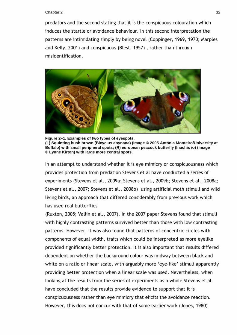
Figure 2–1. Examples of two types of eyespots. (L) Squinting bush brown ( Bicyclus anynana) (Image © 2005 Antónia Monteiro/University at Buffalo) with small peripheral spots; (R) european peacock butterfly ( Inachis io) (Image © Lynne Kirton) with large more central spots.
In an attempt to understand whether it is eye mimicry or conspicuousness which
provides protection from predation Stevens et al have conducted a series of
experiments (Stevens et al., 2009a; Stevens et al., 2009b; Stevens et al., 2008a;
Stevens et al., 2007; Stevens et al., 2008b) using artificial moth stimuli and wild
living birds, an approach that differed considerably from previous work which
has used real butterflies
(Ruxton, 2005; Vallin et al., 2007). In the 2007 paper Stevens found that stimuli
with highly contrasting patterns survived better than those with low contrasting
patterns. However, it was also found that patterns of concentric circles with
components of equal width, traits which could be interpreted as more eyelike
provided significantly better protection. It is also important that results differed
dependent on whether the background colour was midway between black and
white on a ratio or linear scale, with arguably more ‘eye-like’ stimuli apparently
providing better protection when a linear scale was used. Nevertheless, when
looking at the results from the series of experiments as a whole Stevens et al
have concluded that the results provide evidence to support that it is
conspicuousness rather than eye mimicry that elicits the avoidance reaction.
However, this does not concur with that of some earlier work (Jones, 1980)
Chapter 2 33
where the results were determined to be showing eye mimicry is key to the
avoidance response (Appendix ii for full comparison).
In Stevens et al 2009 paper they touched on the possibility that the apparent
direction of gaze may be a possible contributing factor to predator avoidance. It
has been shown that a number avian species are able to react to and follow
human gaze (Bugnyar et al., 2004; Hampton, 1994) and in a recent study it has
been shown that wild-caught European starlings (Sturnus vulgaris) are sensitive
to a predators’ direction of gaze, with a direct gaze resulting in increased time
to feeding resumption, reduced feeding rate and a reduced amount of food
consumed overall (Carter et al., 2008). Work with species as diverse as domestic
chickens, jewelfish and mouse lemurs (Microcebus murinus) has suggested that
eye contact or direct gaze is avoided (Coss, 1978, 1979; Gallup et al., 1972; Lill,
1968; McBride et al., 1963) showing that it may represent an aversive event.
These results suggest that if eyespots are being responded to as eye mimics and
not as conspicuous patterns, we may be able to manipulate predation rate by
changing the apparent direction of the ‘eyespots’ gaze. With this in mind we
plan to test the null hypothesis that apparent direction of gaze has no influence
on prey survival, and the alternative hypothesis that an apparent ‘staring’ or
‘straight’ gaze will work to reduce predation risk. For the null hypothesis to be
rejected we would require that there be a significant difference in survival rates
between the different treatments. For the alternative hypothesis to be accepted
we would have to find that there is a significant reduction in predation risk for
those stimuli with the ‘staring’ or ‘straight’ gaze in comparison to the other
stimuli.
Chapter 2 34
2.1.1 Materials & Methods
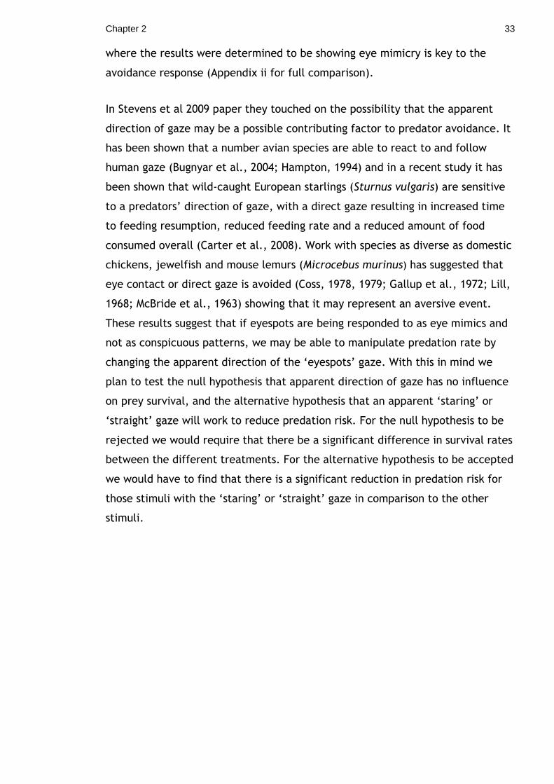
This experiment was conducted in mixed deciduous woodland across 3 sites
within the city of Glasgow, Strathclyde, UK. The data was collected over 2
seasons with the a short pilot study of 4 trials carried out between 25th June
2009 & 9th July 2009 and the large data set collected between the 4th October
2009 & 15th January 2010 at Pollok Country Park (55°49'53"N, 4°18'28"W, see
Figure 2–2). The second data set was collected from two smaller sites at the
Glasgow Botanic Gardens, Glasgow, UK (55°52'53.57"N, 4°17'28.02"W, see Figure
2–2) and Kelvingrove Park, Glasgow, UK (55°52'24.92"N, 4°16'49.50"W, see
Figure 2–2) between April 26th and July 23rd 2011. The two sites were used
alternately to ensure that each site was free from the artificial stimuli for a
minimum of 72 hours prior to Day 1 of any run. We specifically chose to carry out
the main body of this experiment in winter when wasps would not be active.
This was due to both wasps and birds being capable of entirely removing the bait
from the stimuli and so making it impossible to know which had been
responsible. However, we would not expect wasps to vary in their preference
between stimuli. By carrying out the experiment in winter we were able to
remove this potentially confounding factor.
Figure 2–2. Locations of experimental sites. (L: Pollok Country Park & R: Glasgow Botanic Garden s & Kelvingrove Park)
Artificial baits were made using printed ‘moth’ shapes on Canon matt
photographic paper (MP-101). There were 7 treatments in total (Figure 2–3)
consisting of triangular stimuli 44mm wide at the base and 36mm tall. The
stimuli were given a background colour of grey to ensure they were of a lighter
Chapter 2 35
colour than the trees they would be placed on. This is important as previous
work by Stevens et al. (2008a) has shown that eyespots on background matching
prey may actually increase predation.
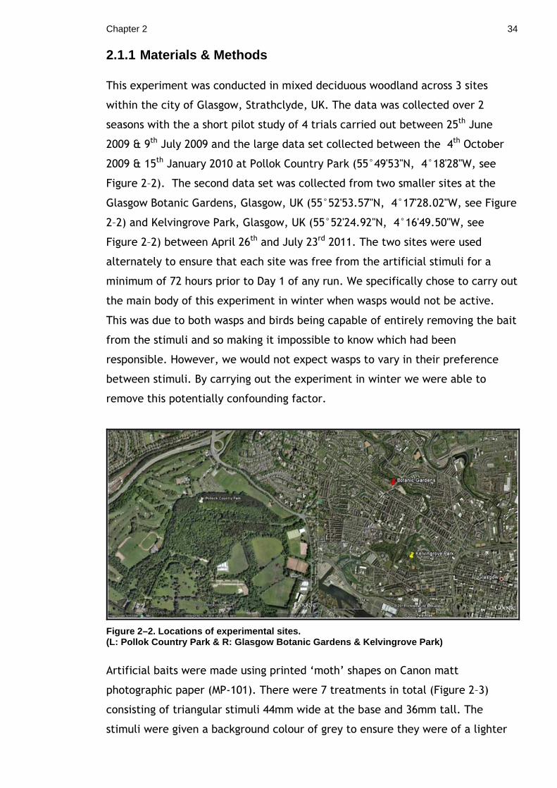
Figure 2–3. Eyegaze stimuli (not actual size). (From left to right stimuli ‘eyes’ are looking; dow n & left (DL); up & left (UL); down & right (DR); up & right (UR); up & out (UO); down & out (D O); straight (S).)
Artificial stimuli with a very basic design were decided upon as this allowed us to
control the levels of contrast and area of ink used. The stimuli designs all use
the same area of ink and had the same contrast, with the only difference
between them the direction of gaze. These 7 stimuli were used to attempt to
mimic all possible gaze directions; from the potentially threatening direct gaze,
looking away, unfocused or not resembling eyes at all. If these stimuli are
perceived as eyes then we might expect that the ‘straight’ stimuli would most
closely resemble direct eye contact or an intense stare of the kind which is
thought to elicit a fear response. The DL & DR and UL & UR are designed to
resemble eyes looking away. The UO & DO are designed to resemble a less direct
gaze or unfocused gaze which may not be perceived as eyes at all. These stimuli
are reasonably similar to the stimuli used by Stevens et al.(2008a).
Our methodology follows the same general procedure as Cuthill et al. (2005)
with the edible component of each bait consisting of a mealworm (Tenebrio
molitor larvae) frozen overnight, then thawed and pinned vertically to the
centre of each stimuli. Meal worms were not used if they were frozen for longer
than 48 hours or reused or refrozen. The mealworms were pinned to the front of
the stimuli to ensure that avian predators (who are unlikely to have encountered
anything similar before) could recognise that they contained an edible
component.
Chapter 2 36
At the start of each trial 70 trees (i.e. 10 replicates of each bait type) were
selected at random with a minimum gap of 10m between them, with only trees
with little or no lichen covering the trunk and of at least 0.9m in circumference
were used. Baits were assigned randomly to a tree (1-70) prior to arriving at the
site and attached a minimum of 1.5m up from the base using dressmaker’s pins.
Randomisation of the allocations was achieved by assigning baits a number
generated by the Excel function RAND() and using the SORT function to put them
in ascending order to be placed on trees 1-70. To aid relocation of the stimuli at
the 2009/2010 season at Pollok Country Park site three mountain bike trails
running through the experimental area were used as guide to pin out, with the
three tracks used sequentially (Figure 2–4) which ensured that there was a
minimum of 6 days between the use of each trail. For the 2011 season the two
sites (Botanical Gardens & Kelvingrove Park) were used alternately which
ensured a minimum of 72 hours between the use of each site. The minimum
distance between each stimuli and the rotation of different trails between trials
are features designed to reduce the likelihood of any one bird encountering
multiple stimuli. It was also decided that, as this area is a popular recreation
area and likely to be particularly busy at the weekends, to reduce disturbance
levels weekends were to be avoided as Day1 of any trial.
Every time the site was visited the date & time of arrival and departure was
noted. Weather conditions and temperature at 9am, 12pm and 5pm were taken
from the Met Office website for each day of the experiment.
Chapter 2 37
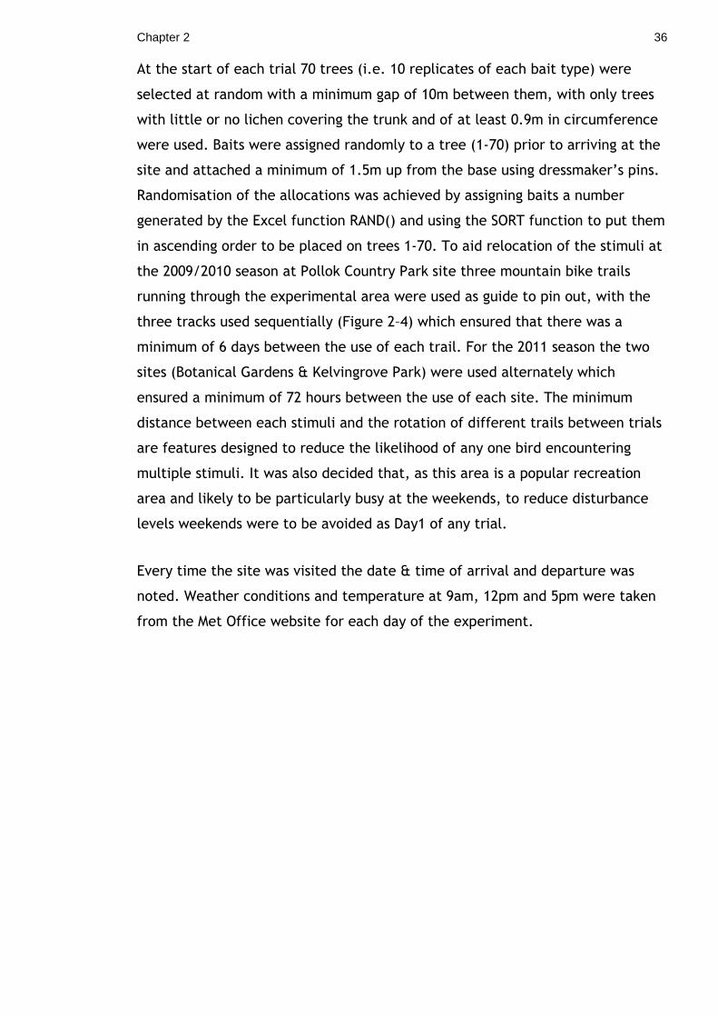
Figure 2–4. Pollok Country Park - Mountain bike tra cks (Image from http://www.flickr.com/photos/defmech/15 4929385/)
The experiment was conducted over 48hrs with the baits put out on the morning
of day 1 and checked for bait survival at 2, 4, 24 and 48hrs. Avian predation was
taken to be indicated by complete or almost complete disappearance of the
mealworm. Non-avian predators such as slugs were indicated by slime trails left
behind and spiders by the baits being sucked dry leaving only hollow
exoskeletons. Harvestmen were also seen eating the baits but similar to the
spiders would eat the insides leaving the exoskeleton. Once all data had been
collected the total number of each stimuli used across all trials was calculated
along with survival and predator type. The predation of the bait by avian and
non-avian predators or the ‘survival’ of the bait to the end of the trial, were all
treated as censored values in the survival analysis.
The survival analysis was conducted in SPSS and a Cox proportional hazards
regression used to accommodate the censored data and the varying predation
risk throughout the day (Cox, 1972; Klein J.P. & Moeschberger, 2003; Lawless,
2002). Significance was then tested using the Wald statistic and effect sizes are
given by the odds ratio (Exp(B)), which is the ratio of the probability of
predation in one treatment to the probability of predation in another treatment.
Chapter 2 38
2.1.2 Results
Although 260 of each stimulus were put out some were dislodged, lost or
damaged due to weather and therefore not included in the final analysis so that
there was a minimum of 254 included for each treatment.
Stimuli Fate
0%
10%
20%
30%
40%
50%
60%
70%
80%
90%
100%
S RD RU LD LU DO UO
Stimuli types
Per
cent
age Survived 48hrs
Predated by 'other'
Avian predation
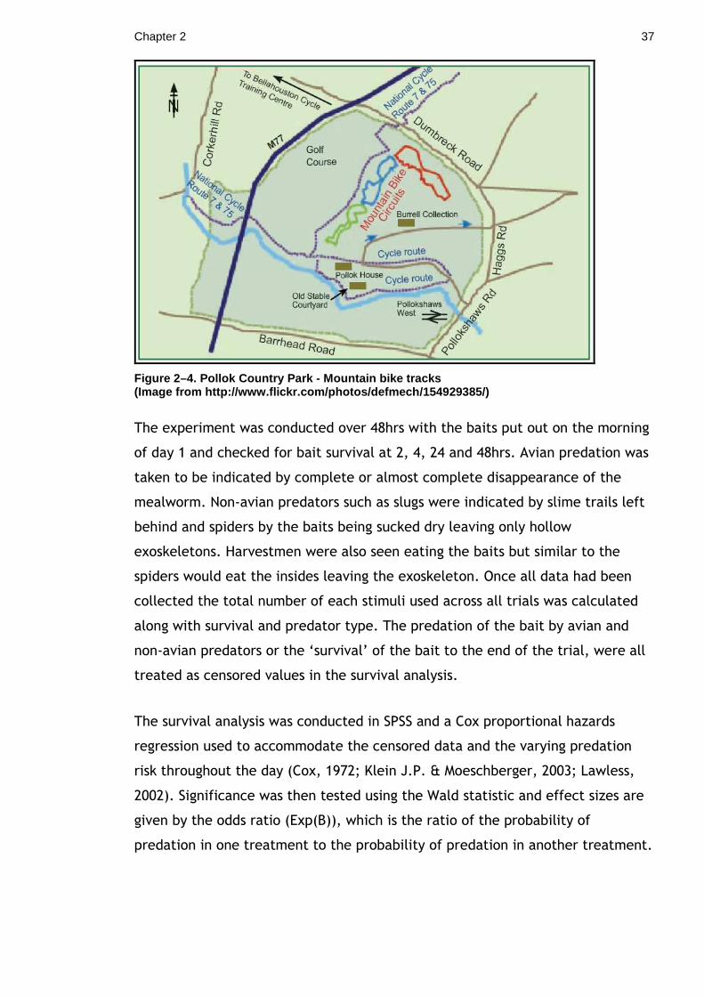
Figure 2–5. Graph depicting the fate of different s timuli types. (S = straight, RD= Right & Down, RU = Right & Up, L D = Left & Down, LU = Left & Up, DO = Down & Out, UO = Up & Out)
Looking at the percentage of the total stimuli that where predated by avian or
‘other’ predators or survived to the end of the 48hrs, we can see here that
roughly 50% of each stimuli type survived to the end of the 48hr trial (Figure 2–
5).
The survival analysis carried out examined each stimulus type when compared to
the stimulus with an apparent ‘straight’ or ‘direct’ gaze. It was found that
survival rates for the downward looking stimuli LD, RD and DO are significantly
different than the S (straight) stimuli with p-values of <0.05 (LD <0.000; RD
<0.000; DO <0.019). The upward looking stimuli LU, RU and UO do not differ
significantly from the S stimuli survival rate.
Chapter 2 39
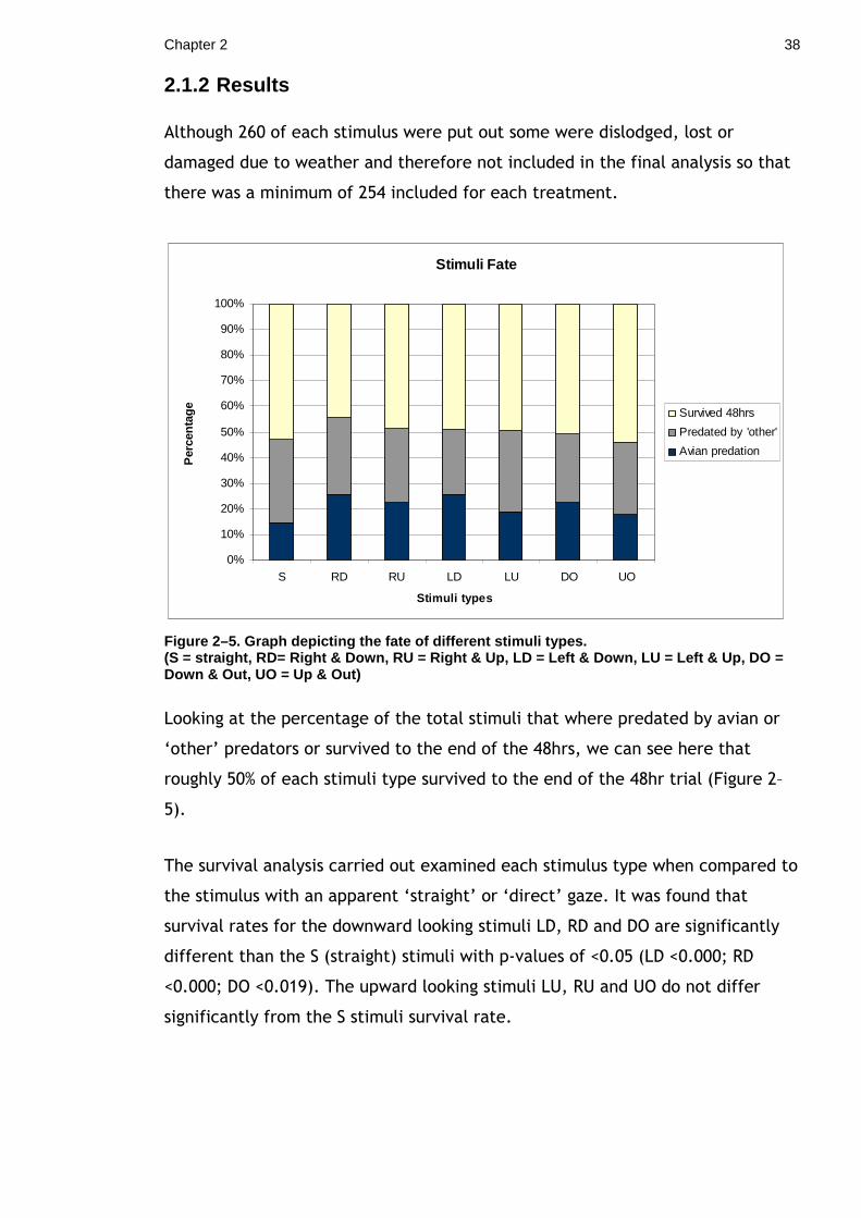
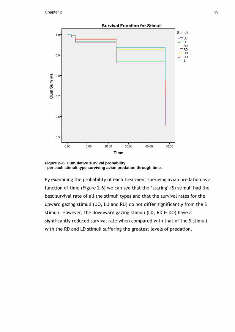
Figure 2–6. Cumulative survival probability - per each stimuli type surviving avian predation t hrough time.
By examining the probability of each treatment surviving avian predation as a
function of time (Figure 2–6) we can see that the ‘staring’ (S) stimuli had the
best survival rate of all the stimuli types and that the survival rates for the
upward gazing stimuli (UO, LU and RU) do not differ significantly from the S
stimuli. However, the downward gazing stimuli (LD, RD & DO) have a
significantly reduced survival rate when compared with that of the S stimuli,
with the RD and LD stimuli suffering the greatest levels of predation.
Chapter 2 40
2.1.3 Discussion
For this experiment we are only interested in those stimuli that were predated
upon by birds, since other predators are not expected to be affected by the
treatments. From (Figure 2–5) we can see that only a small proportion of the
stimuli were taken by birds, with the majority with of the stimuli either
surviving to the end of the 48hr trial (50%) or predated by non-avian predators
such as slugs, harvestmen and spiders (29%). The results of the survival analysis
shows us that the all stimuli with patterns designed to give the impression of a
downward gaze (LD, RD and DO) suffered a greater predation rate than the
stimuli with the direct staring gaze (S) (Figure 2–6). On the other hand, the
stimuli with the upward gazes (LU, RU and UO) showed no significant difference
in predation rate when compared to direct gaze stimuli. As all the stimuli used
were identical in contrast and area of colour, these results would indicate that
the apparent direction of the printed eyes was affecting the predation rates,
with patterns imitating a staring or upward gaze providing a greater degree of
protection from predation than patterns imitating a downward gaze.
One obvious contrast between our study and some previous studies carried out
by other workers was that we experienced considerably smaller predation ratios
with only 21% of the stimuli we used being predated by birds. Other studies such
as Stevens et al. (2009b) had the censored data (not eaten by birds) for two
experiments totalling 27% and 17.3% respectively. This difference may in part be
due to longer trial durations used in some of the previous studies, with Stevens
et al. conducting trials over 48hrs (2008a), 72 hrs (2009a; 2009b) and 96 hrs
(2009b). However, we would argue that by extending the duration of the trials
to achieve a greater predation ratio we risk losing a degree of realism. We must
also consider what might be a ‘normal’ predation rate for a wild population.
Although unable to locate any studies in the UK that look at natural predation
rates for lepidopteran populations we were able to compare our results with a
study examining the predation rates of lepidopteran larvae in a Neoptropical
environment (Koh and Menge, 2006). This study found that predation rates were
anywhere between 30-60%. However, this was not limited to avian predation and
included any predatory attack. Nevertheless, our results fall within these levels
and with some of the previous studies showing what appear to be considerably
higher predation rates. Obviously this is not the most ideal of comparisons and
Chapter 2 41
there are obvious differences between the neotropical forest used in this study
and the highly disturbed temperate woodland used in the UK studies. It is
possible that predation rates experienced may be considerably higher in a
neotropical environment or that the distribution of avian and other predators
differ considerably. For a true picture of what ‘natural’ predation rates are we
really to carry out a similar study within the UK.
The large central eyespots that our stimuli are intended to mimic are, as
discussed previously, thought to be startling when suddenly revealed during an
attack. This means that having the eyespots in full view, motionless and in the
same position for a number of days is a highly unnatural situation, with the
potential for neo-phobic or startle reactions to be overcome due to continued
exposure.
We had anticipated that the staring stimuli would have a greater survival rate,
but these results seem to also indicate a possible difference between the way
the upward and downward stares are being perceived, with the staring and
upward looking stimuli both apparently conferring a greater protective value. To
provide a greater understanding of this result, we feel that future work may
have to look at the angle and height at which birds are first encountering the
stimuli. The stimuli were attached to trees at a minimum of 1.5m, a height
which would mean that the majority of birds would be approaching the stimuli
from above. In this case the upward looking stimuli although not apparently
staring directly at the birds may have appeared more vigilant and therefore
more threatening than the downward looking stimuli. Whatever the mechanism,
this result would lend support to the hypothesis that it is similarity to eyes which
give eyespots their aversive qualities and not conspicuous colouration or
contrast. However, this is not to say that conspicuous colouration has no part to
play as having highly contrasting and conspicuous markings is likely to enhance
and add to any effect.
It would be interesting in future investigations to look more closely at the
apparent difference between the upward and downward looking stimuli. A
potential improvement would be to find some method to control the direction
from which the stimuli are approached and may require an aviary experiment.
Would we for instance still have the same result if the stimuli were approached
Chapter 2 42
from below? The use of motion sensitive photography would allow us to
determine the angle at which birds approach the stimuli and perhaps also
determine how long if at all birds observe the stimuli before attacking. Any
delay in attack, a long observation period or repeated visits before the stimuli is
attacked might give us a greater insight into how the patterns affect predation.
It is also generally assumed that eyespots are startling due to their resemblance
to the predator’s own predators, with staring stimuli most closely resembling an
actively hunting predator. However, our results might hint at some aspect of
implied vigilance, with predators perhaps less willing to attack an apparently
vigilant prey? We may also want to investigate whether all eyes are equally
startling i.e. predator vs. non-predator eyes. Birds of prey and big cats have
often been noted to have highly conspicuously coloured irises surrounding a dark
and strongly contrasting pupil and although this has been touched on to some
extent by Stevens et al. (2009), it may be of interest to examine in more detail
whether this type of eye is any more startling or aversive than the eyes of non-
predatory species. Another potential avenue of investigation is to look at the
evidence that “bigger may be better”, with larger eyespots potentially providing
greater protection. The theory behind this hypothesis is that larger eyes may be
used to estimate the size of the animals, with larger eyes indicating a larger
animal and potential more dangerous predator. Again, this has been touched on
by Stevens et al. (2008b), but has also been suggested by work with reptiles
(Burger et al., 1991) which were shown to flee more quickly in response to a
large rather than a small eye.
We chose, in this instance, to test our hypothesis in a field rather than lab
setting as this adds a degree of realism to the setting that we could not replicate
in the lab. However, there are several problems with this approach that limit
how we can interpret that data. The stimuli we used are not ‘real’ butterflies
and so we can not be sure that the birds interacting with them as they would a
real butterfly. The larger, more eye like, eyespots that we are attempting to
investigate are the type that are usually revealed suddenly or flashed at an
attacker in order to startle, but our eyespots were on continuous display and
motionless and therefore not being seen as they would in nature.

Chapter 2 43
A potential middle ground between the lab and field studies would be an aviary
study using wild caught birds. An aviary would allow us greater control over the
environment, while still retaining a degree of realism when compared to lab
studies. We would be better able to exclude non-avian predators and be certain
that any bait taken was indeed removed by a bird. We would also be able to
observe a bird’s behaviour before removing the bait. Do they observe the bait
from a distance first and from what angle do they approach? A further
improvement would be to better mimic the behaviour of the model butterflies
with eyespots that are suddenly revealed when a bird approaches.
As can be seen from the above there is still a large amount of work that needs to
be done to disentangle the effects of conspicuousness and eye mimicry. What do
predators use to identify eyes, if they do at all? There is of course the possibility
that eyespots are effective because they are conspicuous and that eye mimicry
increases their effectiveness in certain circumstances.
In conclusion, while there still much more worked needing to be done our
findings that the apparent direction of gaze affects predation rates, is evidence
that at least in some cases eyespots may be being perceived as eyes and not
simply as a conspicuous pattern.
Chapter 2 44
2.2 Does the direct gaze of a predator have any cos ts to prey?
Aversion to two facing eyes can be found throughout the animal kingdom, with
species of fish, mammals and birds all shown to show some kind of innate
aversion or flight response to their presence (Coss, 1978, 1979; Hampton, 1994;
Jones, 1980; Stevens, 2005). In almost all of these experiments the greatest
responses have been elicited from paired horizontally orientated stimuli, but
have varied from simple black dots or concentric circles to a real human gaze.
The apparent ubiquity of this response would seem to indicate that aversion to
gaze is perhaps an important and primitive defensive mechanism. In fact
eyespots are well known to be used by both Lepidopteran and fish species to
intimidate or startle predators allowing them time to escape, although the
mechanism is still being debated and not all researchers argue that intimidation
is achieved by mimicry of a potential predator’s eyes (see Stevens, 2005).
Primates have been shown to have a strong bias towards looking at the eyes
when presented with faces of their own and other primate species (Emery,
2000). Humans also show a strong response to the gaze of another with evidence
that people are both more generous and more honest when being ‘watched’ by
the image of a pair of eyes (Bateson et al., 2006; Haley and Fessler, 2005), a
reaction which appears to be entirely unconscious. An interesting aspect is that
it is not necessary for the image used to be photographic or realistic as, Haley &
Fessler were able to elicit a response using a stylised image. It also appears that
we find it extremely difficult to ignore a direct gaze, with a recent paper (Conty
et al., 2010) suggesting that we find it almost impossible to refrain from
processing a direct gaze even when concentrating on another task.
PET scans have been used to investigate brain activation when carrying out
discrimination tasks between eye-contact and no eye-contact conditions. It was
found that the amygdala showed significant activation, with the left active in
both conditions and the right during the eye-contact condition(Kawashima et al.,
1999). The amygdala is responsible for some of our more primitive and
instinctual responses such as the fight or flight response. That eye-contact is
able to activate this area of the brain may suggests that it has an important and
perhaps primitive role. For the most part experiments investigating human
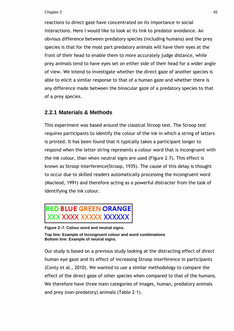
Chapter 2 45
reactions to direct gaze have concentrated on its importance in social
interactions. Here I would like to look at its link to predator avoidance. An
obvious difference between predatory species (including humans) and the prey
species is that for the most part predatory animals will have their eyes at the
front of their head to enable them to more accurately judge distance, while
prey animals tend to have eyes set on either side of their head for a wider angle
of view. We intend to investigate whether the direct gaze of another species is
able to elicit a similar response to that of a human gaze and whether there is
any difference made between the binocular gaze of a predatory species to that
of a prey species.
2.2.1 Materials & Methods
This experiment was based around the classical Stroop test. The Stroop test
requires participants to identify the colour of the ink in which a string of letters
is printed. It has been found that it typically takes a participant longer to
respond when the letter string represents a colour word that is incongruent with
the ink colour, than when neutral signs are used (Figure 2–7). This effect is
known as Stroop interference(Stroop, 1935). The cause of this delay is thought
to occur due to skilled readers automatically processing the incongruent word
(Macleod, 1991) and therefore acting as a powerful distracter from the task of
identifying the ink colour.
Figure 2–7. Colour word and neutral signs.
Top line: Example of incongruent colour and word co mbinations Bottom line: Example of neutral signs.
Our study is based on a previous study looking at the distracting effect of direct
human eye gaze and its effect of increasing Stroop interference in participants
(Conty et al., 2010). We wanted to use a similar methodology to compare the
effect of the direct gaze of other species when compared to that of the humans.
We therefore have three main categories of images, human, predatory animals
and prey (non-predatory) animals (Table 2–1).
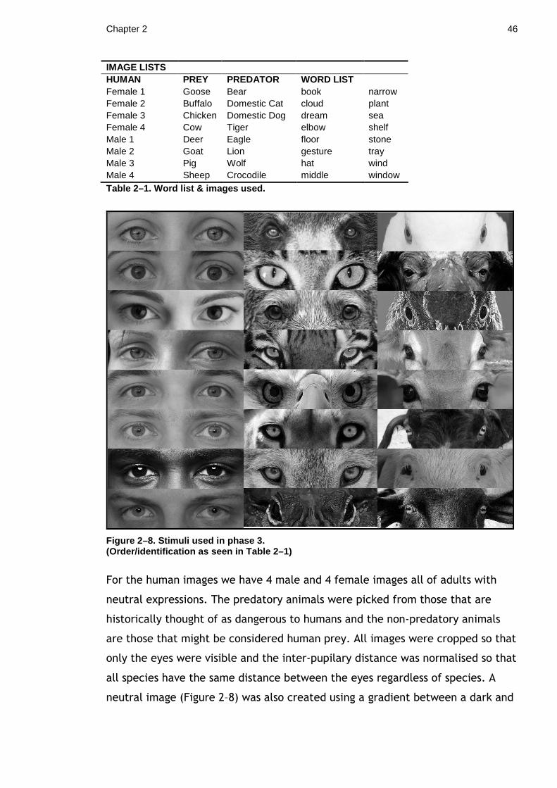
Chapter 2 46
IMAGE LISTS HUMAN PREY PREDATOR WORD LIST Female 1 Goose Bear book narrow Female 2 Buffalo Domestic Cat cloud plant Female 3 Chicken Domestic Dog dream sea Female 4 Cow Tiger elbow shelf Male 1 Deer Eagle floor stone Male 2 Goat Lion gesture tray Male 3 Pig Wolf hat wind Male 4 Sheep Crocodile middle window Table 2–1. Word list & images used.
Figure 2–8. Stimuli used in phase 3. (Order/identification as seen in Table 2–1)
For the human images we have 4 male and 4 female images all of adults with
neutral expressions. The predatory animals were picked from those that are
historically thought of as dangerous to humans and the non-predatory animals
are those that might be considered human prey. All images were cropped so that
only the eyes were visible and the inter-pupilary distance was normalised so that
all species have the same distance between the eyes regardless of species. A
neutral image (Figure 2–8) was also created using a gradient between a dark and
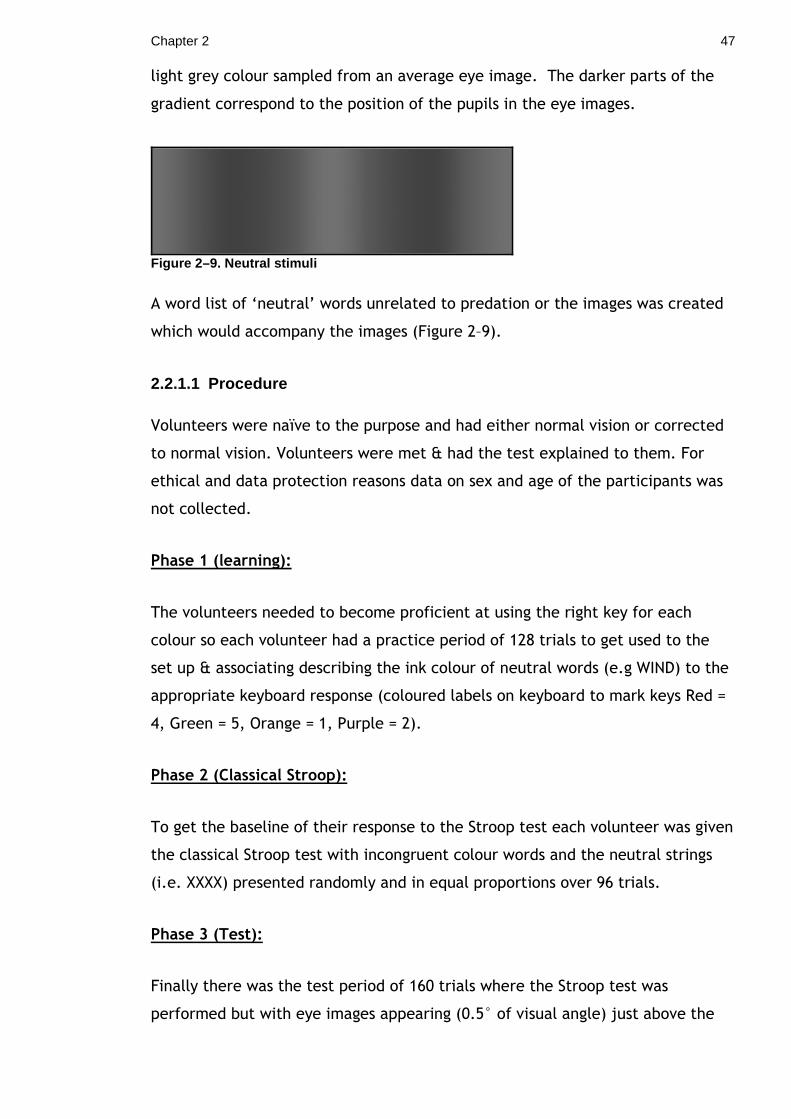
Chapter 2 47
light grey colour sampled from an average eye image. The darker parts of the
gradient correspond to the position of the pupils in the eye images.
Figure 2–9. Neutral stimuli
A word list of ‘neutral’ words unrelated to predation or the images was created
which would accompany the images (Figure 2–9).
2.2.1.1 Procedure
Volunteers were naïve to the purpose and had either normal vision or corrected
to normal vision. Volunteers were met & had the test explained to them. For
ethical and data protection reasons data on sex and age of the participants was
not collected.
Phase 1 (learning):
The volunteers needed to become proficient at using the right key for each
colour so each volunteer had a practice period of 128 trials to get used to the
set up & associating describing the ink colour of neutral words (e.g WIND) to the
appropriate keyboard response (coloured labels on keyboard to mark keys Red =
4, Green = 5, Orange = 1, Purple = 2).
Phase 2 (Classical Stroop):
To get the baseline of their response to the Stroop test each volunteer was given
the classical Stroop test with incongruent colour words and the neutral strings
(i.e. XXXX) presented randomly and in equal proportions over 96 trials.
Phase 3 (Test):
Finally there was the test period of 160 trials where the Stroop test was
performed but with eye images appearing (0.5° of visual angle) just above the
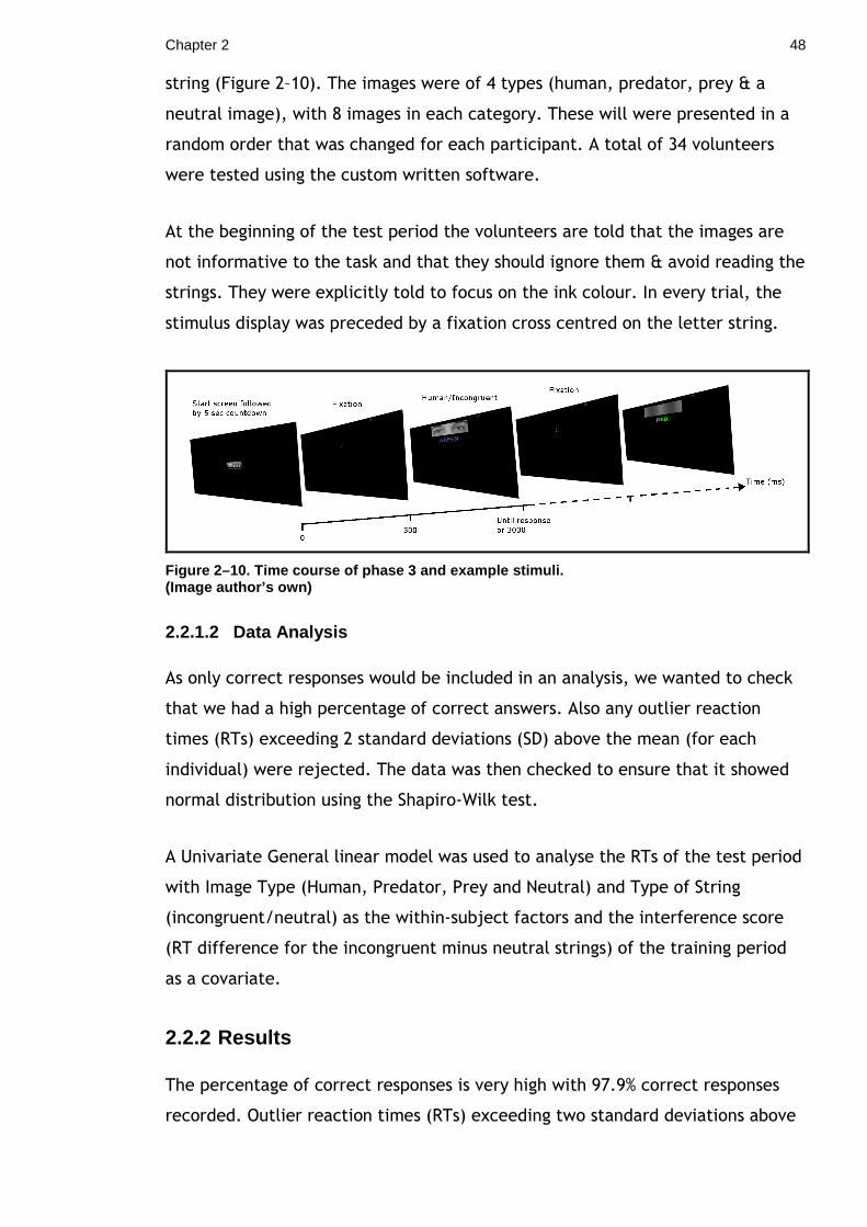
Chapter 2 48
string (Figure 2–10). The images were of 4 types (human, predator, prey & a
neutral image), with 8 images in each category. These will were presented in a
random order that was changed for each participant. A total of 34 volunteers
were tested using the custom written software.
At the beginning of the test period the volunteers are told that the images are
not informative to the task and that they should ignore them & avoid reading the
strings. They were explicitly told to focus on the ink colour. In every trial, the
stimulus display was preceded by a fixation cross centred on the letter string.
Figure 2–10. Time course of phase 3 and example sti muli. (Image author’s own)
2.2.1.2 Data Analysis
As only correct responses would be included in an analysis, we wanted to check
that we had a high percentage of correct answers. Also any outlier reaction
times (RTs) exceeding 2 standard deviations (SD) above the mean (for each
individual) were rejected. The data was then checked to ensure that it showed
normal distribution using the Shapiro-Wilk test.
A Univariate General linear model was used to analyse the RTs of the test period
with Image Type (Human, Predator, Prey and Neutral) and Type of String
(incongruent/neutral) as the within-subject factors and the interference score
(RT difference for the incongruent minus neutral strings) of the training period
as a covariate.
2.2.2 Results
The percentage of correct responses is very high with 97.9% correct responses
recorded. Outlier reaction times (RTs) exceeding two standard deviations above
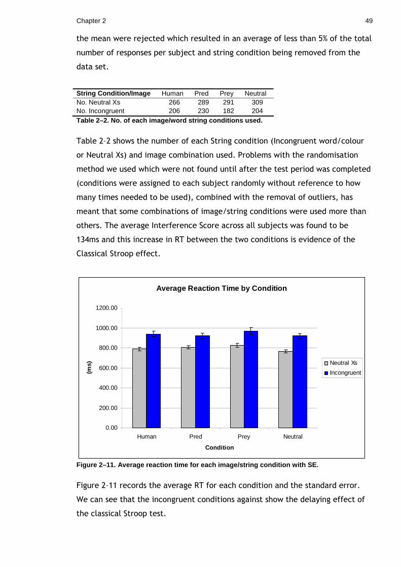
Chapter 2 49
the mean were rejected which resulted in an average of less than 5% of the total
number of responses per subject and string condition being removed from the
data set.
String Condition/Image Human Pred Prey Neutral No. Neutral Xs 266 289 291 309 No. Incongruent 206 230 182 204 Table 2–2. No. of each image/word string conditions used.
Table 2–2 shows the number of each String condition (Incongruent word/colour
or Neutral Xs) and image combination used. Problems with the randomisation
method we used which were not found until after the test period was completed
(conditions were assigned to each subject randomly without reference to how
many times needed to be used), combined with the removal of outliers, has
meant that some combinations of image/string conditions were used more than
others. The average Interference Score across all subjects was found to be
134ms and this increase in RT between the two conditions is evidence of the
Classical Stroop effect.
Average Reaction Time by Condition
0.00
200.00
400.00
600.00
800.00
1000.00
1200.00
Human Pred Prey Neutral
Condition
(ms) Neutral Xs
Incongruent
Figure 2–11. Average reaction time for each image/s tring condition with SE.
Figure 2–11 records the average RT for each condition and the standard error.
We can see that the incongruent conditions against show the delaying effect of
the classical Stroop test.
Chapter 2 50
We checked for normal distribution using the Shapiro-Wilk Test as this is more
appropriate for small sample sizes (< 50 samples) but can also handle sample
sizes as large as 2000. For this reason, we used the Shapiro-Wilk test as our
numerical means of assessing normality. The data we used was the square root
of the average RT per subject, per condition.
The Incon-Human, Incon-Pred and NeutralX-Neutral conditions were found to
significantly deviate from a normal distribution (Incon-Human, W= 0.94, d.f. =
37, p = 0.03; NeutralX-Human, W= 0.98, d.f. = 37, p = 0.76; Incon-Pred, W=
0.93, d.f. = 37, p = 0.03 ; NeutralX-Pred, W= 0.96, d.f. = 37, p = 0.18; Incon-
Prey, W= 0.96, d.f. = 37, p = 0.18; NeutralX-Prey, W= 0.99, d.f. = 37, p = 0.88;
Incon-Neutral, W= 0.12, d.f. = 37, p = 0.17; and NeutralX-Neutral, W= 0.92, d.f.
= 37, p = 0.015). Although not all of our data is normal, we have used a General
Linear Model to analyse our data and they are known to be robust in dealing with
non-normal data distributions.
From the analysis we found no significant interactions for any of the conditions
tested and thus there is no evidence that the subjects were distracted
differentially by the different types of image (GLM, F = 0.131, p = 0.94)
2.2.3 Discussion
As expected out participants showed the classical Stroop interference. However,
the type of eyes above the strings had absolutely no effect on the size of the
Stroop effect. This does not match the results reported in Conty et al’s (2010)
study, where it was found that direct human eye contact significantly increased
the size of the Stroop effect. In this study neither the human, animal or neutral
image had any significant effect.
As mentioned previously (Chapter 2.1), direct gaze has a measurable effect in
other species with species as diverse as domestic chickens, jewelfish and mouse
lemurs (Microcebus murinus) finding that eye contact or direct gaze is avoided
(Coss, 1978, 1979; Gallup et al., 1972; Lill, 1968; McBride et al., 1963) and may
represent an aversive event. There is also work that shows that this effect can
be seen across species with a number of avian species able to react to and
follow human gaze (Bugnyar et al., 2004; Hampton, 1994). In a recent study it
Chapter 2 51
was shown that wild-caught European starlings (Sturnus vulgaris) are sensitive to
a predators’ direction of gaze, with a direct gaze resulting in increased time to
feeding resumption, reduced feeding rate and a reduced amount of food
consumed overall (Carter et al., 2008).
With this evidence and what we know about the effect of the gaze of other
humans has (Bateson et al., 2006; Haley and Fessler, 2005) it may be too early
to determine that there definitely no effect to be found here. It is possible that
the effect we were looking for is too small to be found with this sample size or
that some aspect of our experimental set up meant that we were unable to
replicate the previous study’s results and it would be prudent to attempt to
repeat this experiment to be sure that this is not the case.
Eyespots are a common component of the aposematic or startling displays and in
particular within the Lepidoptera (Ruxton et al., 2004; Stevens, 2005) and there
is debate as to whether these eyespots are intimidating due to their
resemblance to the eyes of the predators’ own predators or that it is their
conspicuous colouration that induces the startle or avoidance behaviour. In this
second interpretation the patterns are intimidating simply by being novel
(Coppinger, 1969, 1970; Marples and Kelly, 2001) and conspicuous (Blest, 1957) ,
rather than through misidentification. If we are able to accurately measure the
response to real eyes, we might be able to use this approach to test whether
humans respond to Lepidopteran eyespots in the same way.
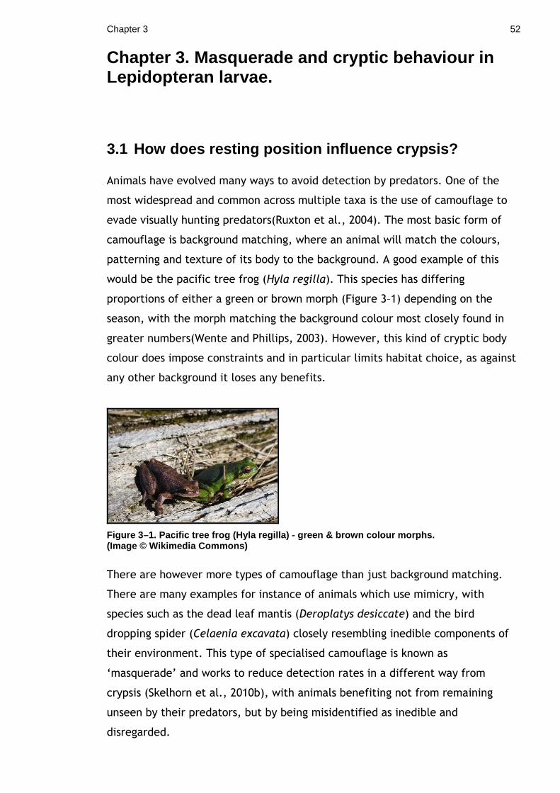
Chapter 3 52
Chapter 3. Masquerade and cryptic behaviour in Lepidopteran larvae.
3.1 How does resting position influence crypsis?
Animals have evolved many ways to avoid detection by predators. One of the
most widespread and common across multiple taxa is the use of camouflage to
evade visually hunting predators(Ruxton et al., 2004). The most basic form of
camouflage is background matching, where an animal will match the colours,
patterning and texture of its body to the background. A good example of this
would be the pacific tree frog (Hyla regilla). This species has differing
proportions of either a green or brown morph (Figure 3–1) depending on the
season, with the morph matching the background colour most closely found in
greater numbers(Wente and Phillips, 2003). However, this kind of cryptic body
colour does impose constraints and in particular limits habitat choice, as against
any other background it loses any benefits.
Figure 3–1. Pacific tree frog ( Hyla regilla) - green & brown colour morphs. (Image © Wikimedia Commons)
There are however more types of camouflage than just background matching.
There are many examples for instance of animals which use mimicry, with
species such as the dead leaf mantis (Deroplatys desiccate) and the bird
dropping spider (Celaenia excavata) closely resembling inedible components of
their environment. This type of specialised camouflage is known as
‘masquerade’ and works to reduce detection rates in a different way from
crypsis (Skelhorn et al., 2010b), with animals benefiting not from remaining
unseen by their predators, but by being misidentified as inedible and
disregarded.
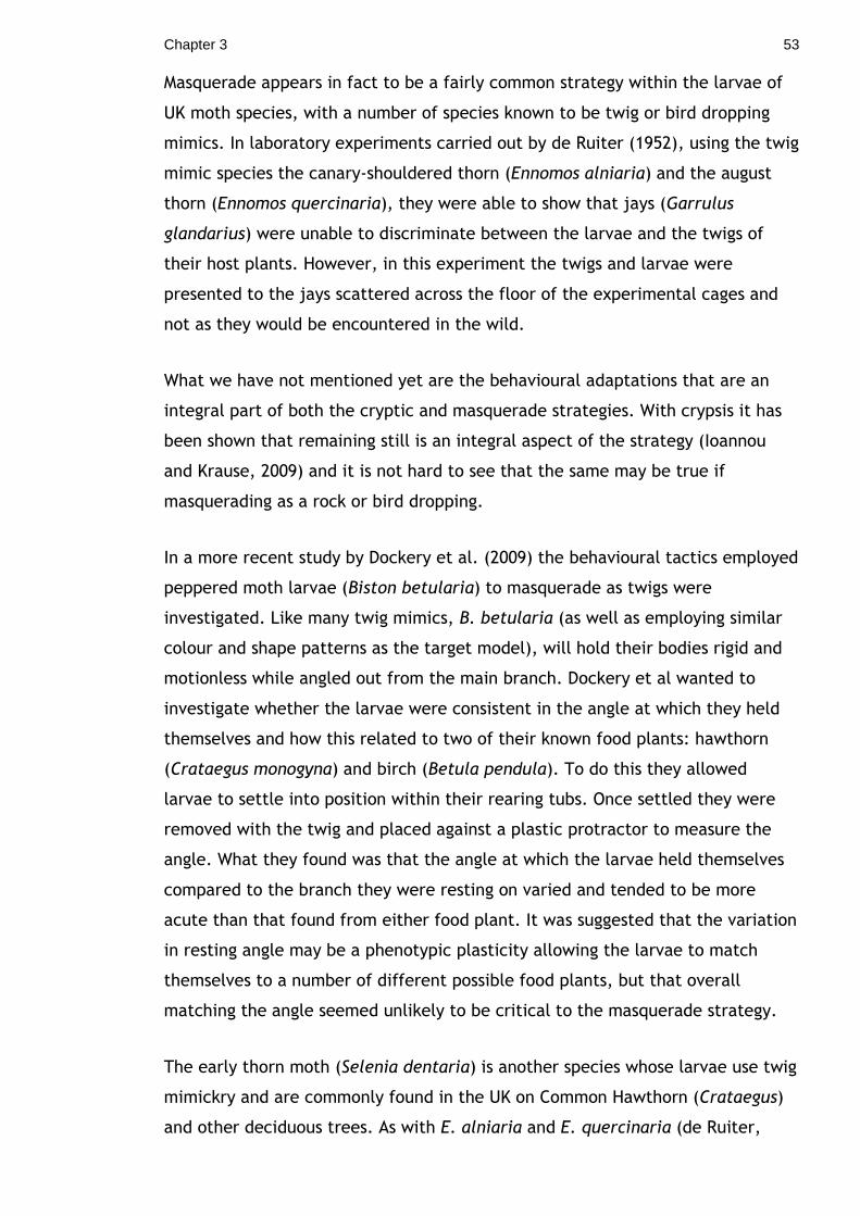
Chapter 3 53
Masquerade appears in fact to be a fairly common strategy within the larvae of
UK moth species, with a number of species known to be twig or bird dropping
mimics. In laboratory experiments carried out by de Ruiter (1952), using the twig
mimic species the canary-shouldered thorn (Ennomos alniaria) and the august
thorn (Ennomos quercinaria), they were able to show that jays (Garrulus
glandarius) were unable to discriminate between the larvae and the twigs of
their host plants. However, in this experiment the twigs and larvae were
presented to the jays scattered across the floor of the experimental cages and
not as they would be encountered in the wild.
What we have not mentioned yet are the behavioural adaptations that are an
integral part of both the cryptic and masquerade strategies. With crypsis it has
been shown that remaining still is an integral aspect of the strategy (Ioannou
and Krause, 2009) and it is not hard to see that the same may be true if
masquerading as a rock or bird dropping.
In a more recent study by Dockery et al. (2009) the behavioural tactics employed
peppered moth larvae (Biston betularia) to masquerade as twigs were
investigated. Like many twig mimics, B. betularia (as well as employing similar
colour and shape patterns as the target model), will hold their bodies rigid and
motionless while angled out from the main branch. Dockery et al wanted to
investigate whether the larvae were consistent in the angle at which they held
themselves and how this related to two of their known food plants: hawthorn
(Crataegus monogyna) and birch (Betula pendula). To do this they allowed
larvae to settle into position within their rearing tubs. Once settled they were
removed with the twig and placed against a plastic protractor to measure the
angle. What they found was that the angle at which the larvae held themselves
compared to the branch they were resting on varied and tended to be more
acute than that found from either food plant. It was suggested that the variation
in resting angle may be a phenotypic plasticity allowing the larvae to match
themselves to a number of different possible food plants, but that overall
matching the angle seemed unlikely to be critical to the masquerade strategy.
The early thorn moth (Selenia dentaria) is another species whose larvae use twig
mimickry and are commonly found in the UK on Common Hawthorn (Crataegus)
and other deciduous trees. As with E. alniaria and E. quercinaria (de Ruiter,
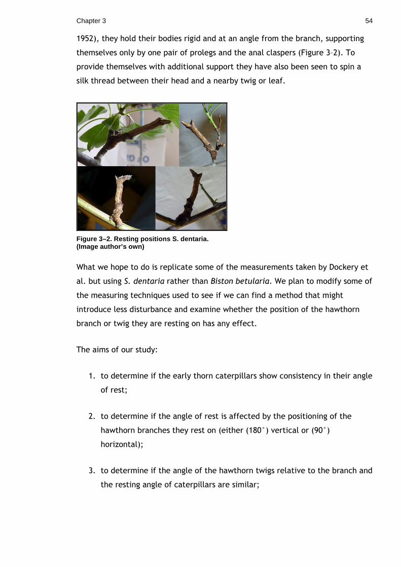
Chapter 3 54
1952), they hold their bodies rigid and at an angle from the branch, supporting
themselves only by one pair of prolegs and the anal claspers (Figure 3–2). To
provide themselves with additional support they have also been seen to spin a
silk thread between their head and a nearby twig or leaf.
Figure 3–2. Resting positions S. dentaria. (Image author’s own)
What we hope to do is replicate some of the measurements taken by Dockery et
al. but using S. dentaria rather than Biston betularia. We plan to modify some of
the measuring techniques used to see if we can find a method that might
introduce less disturbance and examine whether the position of the hawthorn
branch or twig they are resting on has any effect.
The aims of our study:
1. to determine if the early thorn caterpillars show consistency in their angle
of rest;
2. to determine if the angle of rest is affected by the positioning of the
hawthorn branches they rest on (either (180°) vertical or (90°)
horizontal);
3. to determine if the angle of the hawthorn twigs relative to the branch and
the resting angle of caterpillars are similar;
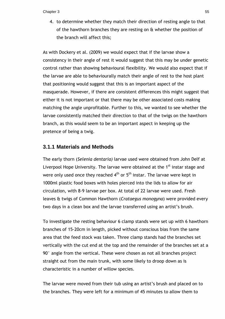
Chapter 3 55
4. to determine whether they match their direction of resting angle to that
of the hawthorn branches they are resting on & whether the position of
the branch will affect this;
As with Dockery et al. (2009) we would expect that if the larvae show a
consistency in their angle of rest it would suggest that this may be under genetic
control rather than showing behavioural flexibility. We would also expect that if
the larvae are able to behaviourally match their angle of rest to the host plant
that positioning would suggest that this is an important aspect of the
masquerade. However, if there are consistent differences this might suggest that
either it is not important or that there may be other associated costs making
matching the angle unprofitable. Further to this, we wanted to see whether the
larvae consistently matched their direction to that of the twigs on the hawthorn
branch, as this would seem to be an important aspect in keeping up the
pretence of being a twig.
3.1.1 Materials and Methods
The early thorn (Selenia dentaria) larvae used were obtained from John Delf at
Liverpool Hope University. The larvae were obtained at the 1st instar stage and
were only used once they reached 4th or 5th instar. The larvae were kept in
1000ml plastic food boxes with holes pierced into the lids to allow for air
circulation, with 8-9 larvae per box. At total of 22 larvae were used. Fresh
leaves & twigs of Common Hawthorn (Crataegus monogyna) were provided every
two days in a clean box and the larvae transferred using an artist’s brush.
To investigate the resting behaviour 6 clamp stands were set up with 6 hawthorn
branches of 15-20cm in length, picked without conscious bias from the same
area that the feed stock was taken. Three clamp stands had the branches set
vertically with the cut end at the top and the remainder of the branches set at a
90° angle from the vertical. These were chosen as not all branches project
straight out from the main trunk, with some likely to droop down as is
characteristic in a number of willow species.
The larvae were moved from their tub using an artist’s brush and placed on to
the branches. They were left for a minimum of 45 minutes to allow them to
Chapter 3 56
settle. Once settled those that were determined to be exhibiting the desired
behavioural response, i.e. with the body rigid and still and held at an angle from
the Hawthorn branch were carefully photographed using a digital camera
(Panasonic DMC-TZ7) so as not to touch or disturb the larvae. Once
photographed the larvae were returned to their tubs. Since no larvae were
photographed more than once in 24 hours and the larvae were free to settle
anywhere they chose each picture was regarded as independent.
The pictures were then sorted into those where the larvae were resting on
vertical (180°) or horizontal (90°) Hawthorn branches (Figure 3–3).
Figure 3–3. Defining resting on 90° and 180° twigs. (Image author’s own)
The digital photographs were then used to determine the angle of the larvae.
This was done using the ‘measure tool’ of the image manipulation program GIMP
2.6 which measures angles and distances (Figure 3–4).
Figure 3–4. Measuring angle in GIMP 2.6. (The angle was measured from a point equidistant be tween the last 2 prolegs along a line as close to the middle of the larvae as possible and a long the plane of the twig.) (Image author’s own)
In order to maximise consistency in measurements all measurements were taken
by the same individual. The first image used was measured 10 times in order to
assess whether the measurements were consistent. The difference between the
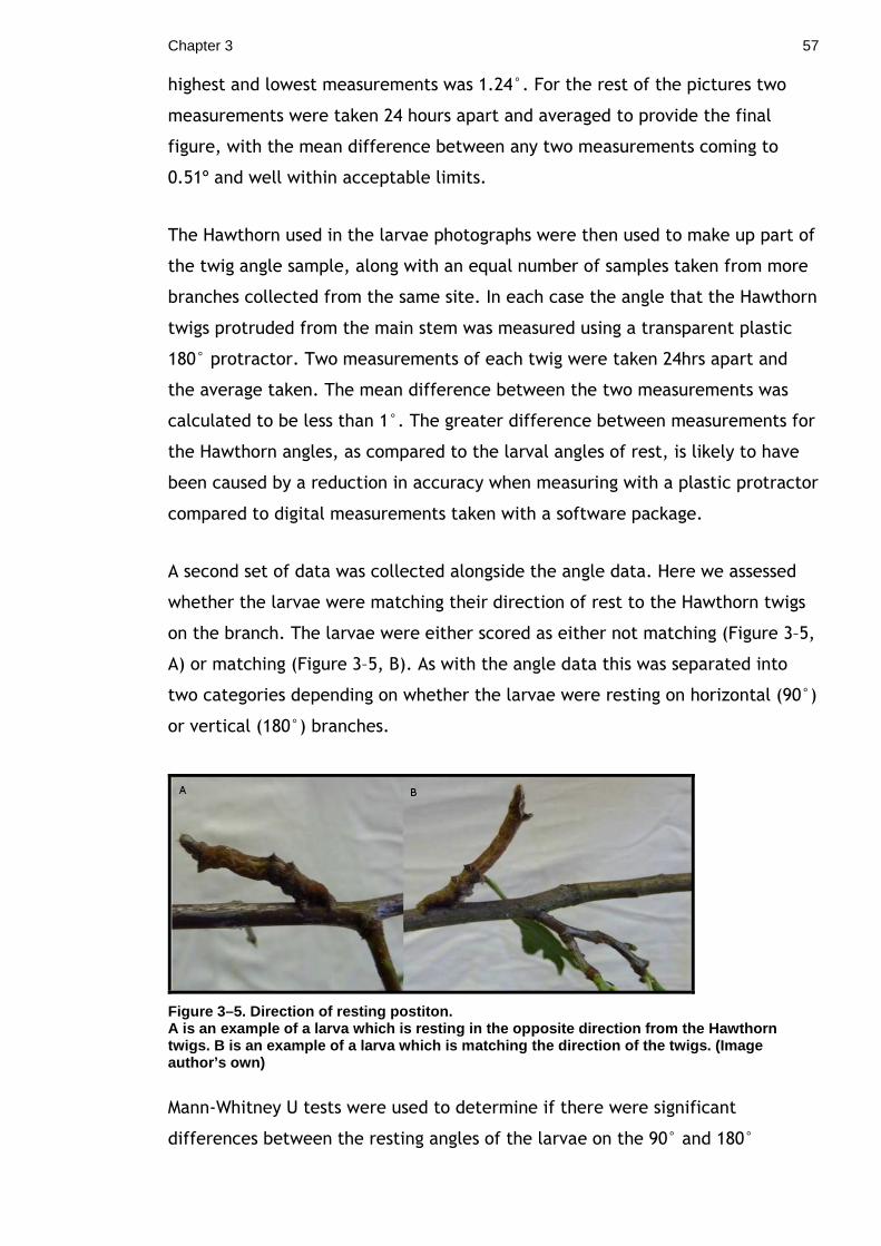
Chapter 3 57
highest and lowest measurements was 1.24°. For the rest of the pictures two
measurements were taken 24 hours apart and averaged to provide the final
figure, with the mean difference between any two measurements coming to
0.51º and well within acceptable limits.
The Hawthorn used in the larvae photographs were then used to make up part of
the twig angle sample, along with an equal number of samples taken from more
branches collected from the same site. In each case the angle that the Hawthorn
twigs protruded from the main stem was measured using a transparent plastic
180° protractor. Two measurements of each twig were taken 24hrs apart and
the average taken. The mean difference between the two measurements was
calculated to be less than 1°. The greater difference between measurements for
the Hawthorn angles, as compared to the larval angles of rest, is likely to have
been caused by a reduction in accuracy when measuring with a plastic protractor
compared to digital measurements taken with a software package.
A second set of data was collected alongside the angle data. Here we assessed
whether the larvae were matching their direction of rest to the Hawthorn twigs
on the branch. The larvae were either scored as either not matching (Figure 3–5,
A) or matching (Figure 3–5, B). As with the angle data this was separated into
two categories depending on whether the larvae were resting on horizontal (90°)
or vertical (180°) branches.
Figure 3–5. Direction of resting postiton. A is an example of a larva which is resting in the opposite direction from the Hawthorn twigs. B is an example of a larva which is matching the direction of the twigs. (Image author’s own)
Mann-Whitney U tests were used to determine if there were significant
differences between the resting angles of the larvae on the 90° and 180°
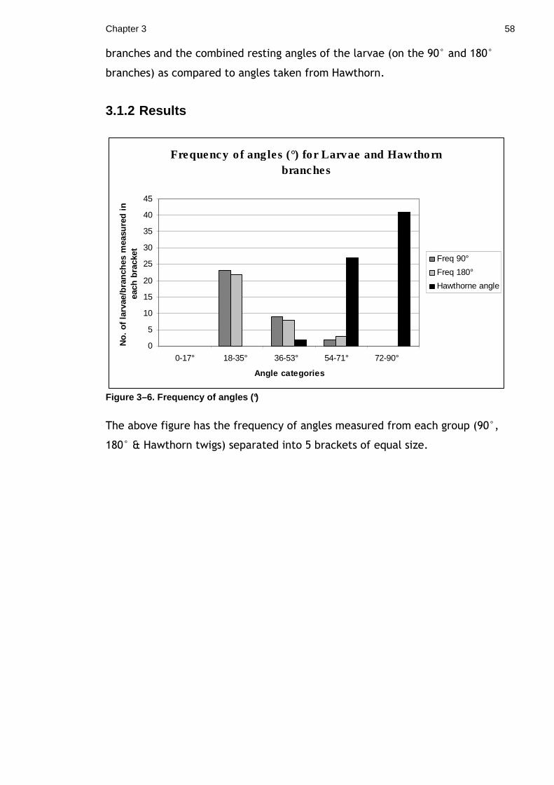
Chapter 3 58
branches and the combined resting angles of the larvae (on the 90° and 180°
branches) as compared to angles taken from Hawthorn.
3.1.2 Results
Frequency of angles (°) for Larvae and Hawthorn branches
0
5
10
15
20
25
30
35
40
45
0-17° 18-35° 36-53° 54-71° 72-90°
Angle categories
No.
of l
arva
e/br
anch
es m
easu
red
in
each
bra
cket Freq 90°
Freq 180°
Hawthorne angle
Figure 3–6. Frequency of angles (°)
The above figure has the frequency of angles measured from each group (90°,
180° & Hawthorn twigs) separated into 5 brackets of equal size.
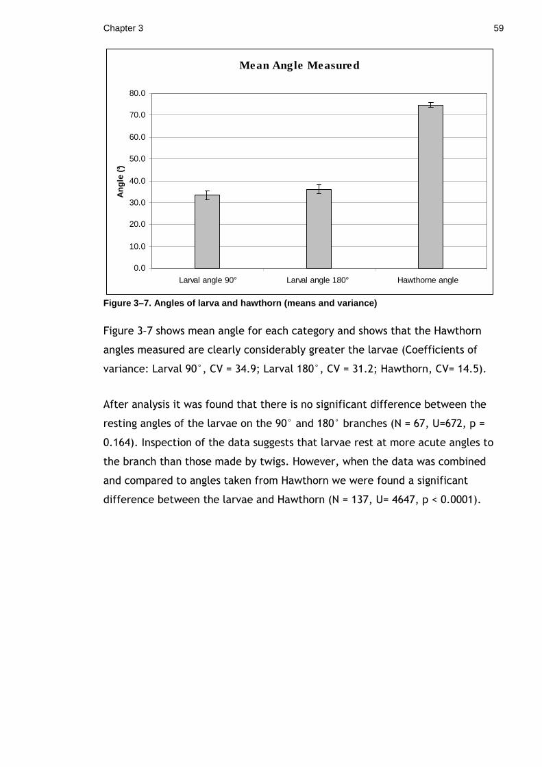
Chapter 3 59
Mean Angle Measured
0.0
10.0
20.0
30.0
40.0
50.0
60.0
70.0
80.0
Larval angle 90° Larval angle 180° Hawthorne angle
Ang
le (
°)
Figure 3–7. Angles of larva and hawthorn (means and variance)
Figure 3–7 shows mean angle for each category and shows that the Hawthorn
angles measured are clearly considerably greater the larvae (Coefficients of
variance: Larval 90°, CV = 34.9; Larval 180°, CV = 31.2; Hawthorn, CV= 14.5).
After analysis it was found that there is no significant difference between the
resting angles of the larvae on the 90° and 180° branches (N = 67, U=672, p =
0.164). Inspection of the data suggests that larvae rest at more acute angles to
the branch than those made by twigs. However, when the data was combined
and compared to angles taken from Hawthorn we were found a significant
difference between the larvae and Hawthorn (N = 137, U= 4647, p < 0.0001).
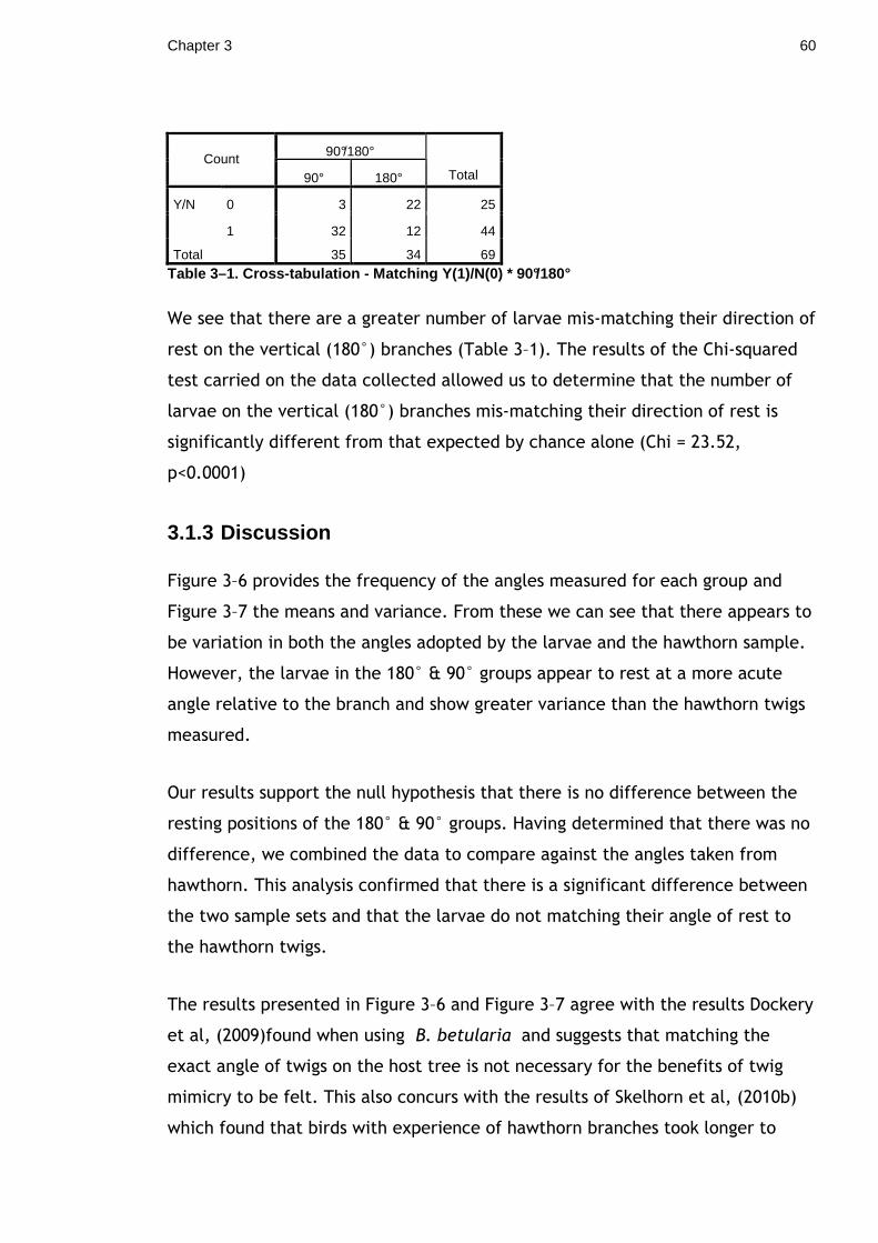
Chapter 3 60
90°/180° Count 90° 180° Total
0 3 22 25 Y/N
1 32 12 44
Total 35 34 69
Table 3–1. Cross-tabulation - Matching Y(1)/N(0) * 90°/180°
We see that there are a greater number of larvae mis-matching their direction of
rest on the vertical (180°) branches (Table 3–1). The results of the Chi-squared
test carried on the data collected allowed us to determine that the number of
larvae on the vertical (180°) branches mis-matching their direction of rest is
significantly different from that expected by chance alone (Chi = 23.52,
p<0.0001)
3.1.3 Discussion
Figure 3–6 provides the frequency of the angles measured for each group and
Figure 3–7 the means and variance. From these we can see that there appears to
be variation in both the angles adopted by the larvae and the hawthorn sample.
However, the larvae in the 180° & 90° groups appear to rest at a more acute
angle relative to the branch and show greater variance than the hawthorn twigs
measured.
Our results support the null hypothesis that there is no difference between the
resting positions of the 180° & 90° groups. Having determined that there was no
difference, we combined the data to compare against the angles taken from
hawthorn. This analysis confirmed that there is a significant difference between
the two sample sets and that the larvae do not matching their angle of rest to
the hawthorn twigs.
The results presented in Figure 3–6 and Figure 3–7 agree with the results Dockery
et al, (2009)found when using B. betularia and suggests that matching the
exact angle of twigs on the host tree is not necessary for the benefits of twig
mimicry to be felt. This also concurs with the results of Skelhorn et al, (2010b)
which found that birds with experience of hawthorn branches took longer to
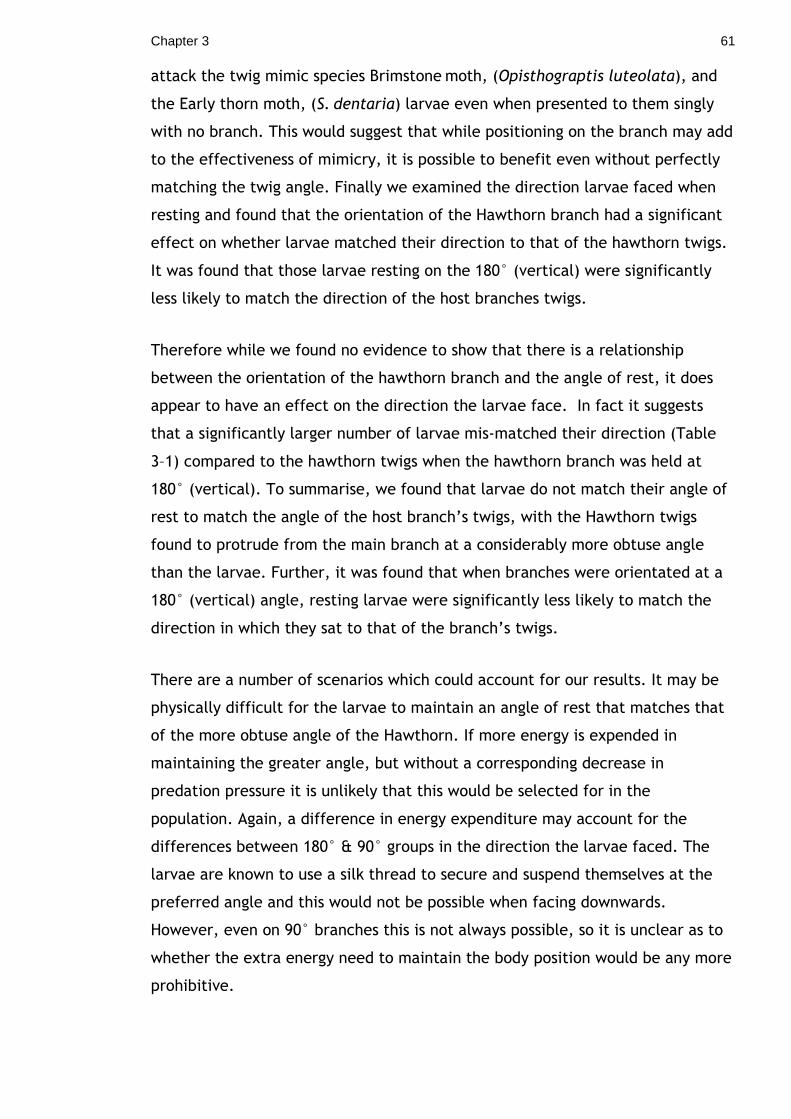
Chapter 3 61
attack the twig mimic species Brimstone moth, (Opisthograptis luteolata), and
the Early thorn moth, (S. dentaria) larvae even when presented to them singly
with no branch. This would suggest that while positioning on the branch may add
to the effectiveness of mimicry, it is possible to benefit even without perfectly
matching the twig angle. Finally we examined the direction larvae faced when
resting and found that the orientation of the Hawthorn branch had a significant
effect on whether larvae matched their direction to that of the hawthorn twigs.
It was found that those larvae resting on the 180° (vertical) were significantly
less likely to match the direction of the host branches twigs.
Therefore while we found no evidence to show that there is a relationship
between the orientation of the hawthorn branch and the angle of rest, it does
appear to have an effect on the direction the larvae face. In fact it suggests
that a significantly larger number of larvae mis-matched their direction (Table
3–1) compared to the hawthorn twigs when the hawthorn branch was held at
180° (vertical). To summarise, we found that larvae do not match their angle of
rest to match the angle of the host branch’s twigs, with the Hawthorn twigs
found to protrude from the main branch at a considerably more obtuse angle
than the larvae. Further, it was found that when branches were orientated at a
180° (vertical) angle, resting larvae were significantly less likely to match the
direction in which they sat to that of the branch’s twigs.
There are a number of scenarios which could account for our results. It may be
physically difficult for the larvae to maintain an angle of rest that matches that
of the more obtuse angle of the Hawthorn. If more energy is expended in
maintaining the greater angle, but without a corresponding decrease in
predation pressure it is unlikely that this would be selected for in the
population. Again, a difference in energy expenditure may account for the
differences between 180° & 90° groups in the direction the larvae faced. The
larvae are known to use a silk thread to secure and suspend themselves at the
preferred angle and this would not be possible when facing downwards.
However, even on 90° branches this is not always possible, so it is unclear as to
whether the extra energy need to maintain the body position would be any more
prohibitive.
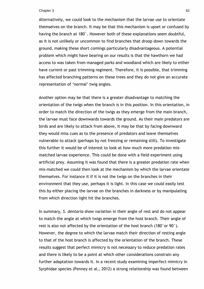
Chapter 3 62
Alternatively, we could look to the mechanism that the larvae use to orientate
themselves on the branch. It may be that this mechanism is upset or confused by
having the branch at 180°. However both of these explanations seem doubtful,
as it is not unlikely or uncommon to find branches that droop down towards the
ground, making these short comings particularly disadvantageous. A potential
problem which might have bearing on our results is that the hawthorn we had
access to was taken from managed parks and woodland which are likely to either
have current or past trimming regiment. Therefore, it is possible, that trimming
has affected branching patterns on these trees and they do not give an accurate
representation of ‘normal’ twig angles.
Another option may be that there is a greater disadvantage to matching the
orientation of the twigs when the branch is in this position. In this orientation, in
order to match the direction of the twigs as they emerge from the main branch,
the larvae must face downwards towards the ground. As their main predators are
birds and are likely to attack from above, it may be that by facing downward
they would miss cues as to the presence of predators and leave themselves
vulnerable to attack (perhaps by not freezing or remaining still). To investigate
this further it would be of interest to look at how much more predation mis-
matched larvae experience. This could be done with a field experiment using
artificial prey. Assuming it was found that there is a greater predation rate when
mis-matched we could then look at the mechanism by which the larvae orientate
themselves. For instance it if it is not the twigs on the branches in their
environment that they use, perhaps it is light. In this case we could easily test
this by either placing the larvae on the branches in darkness or by manipulating
from which direction light hit the branches.
In summary, S. dentaria show variation in their angle of rest and do not appear
to match the angle at which twigs emerge from the host branch. Their angle of
rest is also not affected by the orientation of the host branch (180°or 90°).
However, the degree to which the larvae match their direction of resting angle
to that of the host branch is affected by the orientation of the branch. These
results suggest that perfect mimicry is not necessary to reduce predation rates
and there is likely to be a point at which other considerations constrain any
further adaptation towards it. In a recent study examining imperfect mimicry in
Syrphidae species (Penney et al., 2012) a strong relationship was found between
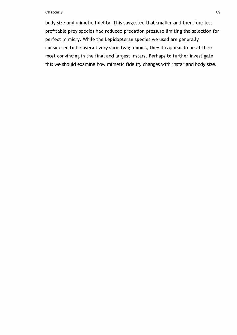
Chapter 3 63
body size and mimetic fidelity. This suggested that smaller and therefore less
profitable prey species had reduced predation pressure limiting the selection for
perfect mimicry. While the Lepidopteran species we used are generally
considered to be overall very good twig mimics, they do appear to be at their
most convincing in the final and largest instars. Perhaps to further investigate
this we should examine how mimetic fidelity changes with instar and body size.
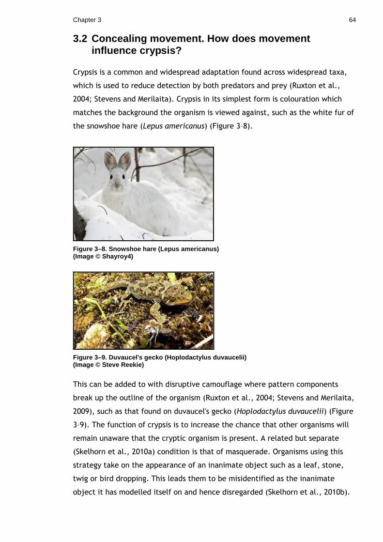
Chapter 3 64
3.2 Concealing movement. How does movement influence crypsis?
Crypsis is a common and widespread adaptation found across widespread taxa,
which is used to reduce detection by both predators and prey (Ruxton et al.,
2004; Stevens and Merilaita). Crypsis in its simplest form is colouration which
matches the background the organism is viewed against, such as the white fur of
the snowshoe hare (Lepus americanus) (Figure 3–8).
Figure 3–8. Snowshoe hare ( Lepus americanus) (Image © Shayroy4)
Figure 3–9. Duvaucel's gecko ( Hoplodactylus duvaucelii) (Image © Steve Reekie)
This can be added to with disruptive camouflage where pattern components
break up the outline of the organism (Ruxton et al., 2004; Stevens and Merilaita,
2009), such as that found on duvaucel's gecko (Hoplodactylus duvaucelii) (Figure
3–9). The function of crypsis is to increase the chance that other organisms will
remain unaware that the cryptic organism is present. A related but separate
(Skelhorn et al., 2010a) condition is that of masquerade. Organisms using this
strategy take on the appearance of an inanimate object such as a leaf, stone,
twig or bird dropping. This leads them to be misidentified as the inanimate
object it has modelled itself on and hence disregarded (Skelhorn et al., 2010b).
Chapter 3 65
Masqueraders are in fact hiding in plain view. Masquerade is about avoiding
being recognised, whereas crypsis is about avoiding being identified as an entity
at all.
The benefits associated with crypsis and masquerade are however likely to come
with associated costs. If you want to be a convincing stone you must have the
associated behavioural traits, which means in this case that any movement may
give the game away. In fact there is evidence to show that once a distant
predator has been detected camouflaged prey will ‘freeze’ (Broom and Ruxton,
2005; Eilam, 2005). Although a long standing belief, with a large body of
anecdotal evidence, there has in fact been little data collected from controlled
experiments to support the importance of stillness to crypsis. However, in a
recent paper Ioannou and Krause (2009) were able to test this hypothesis with
the use of three-spined sticklebacks and their chironomid larvae prey presented
against a red (cryptic) or white (conspicuous) background. The effects of both
background matching and motion were compared as to their effect on detection
rates. Ioannou and Krause were able to show that for crypsis to be effective
background matching needs to be coupled with remaining motionless and that
movement significantly increases detection by predators. This restriction on
movement of course has a significant impact on an organism’s ability to perform
a number of tasks including foraging for resources, mate finding, and adopting a
preferred microclimate in response to changing environmental conditions.
However, for those organisms using masquerade there may be some contexts in
which movement may occur without reducing the effectiveness of masquerade.
Examples may be founding in leaf and twig mimics, such as stick insects and
mantids both of which are known to walk with low amplitude swaying
movements which may be a form of movement concealment (Edmunds and
Brunner, 1999; Robinson, 1966), where the swaying movement may enhance
resemblance by imitating the effect of wind on the leafs or twigs(Bedford, 1978;
Cott, 1940). The mantid Hierodula patellifera is a well-documented leaf mimic,
a strategy used to reduce detection by both potential prey and predators. In a
recent study it was found that both in the field and under laboratory conditions
walking and swaying were more frequently observed in windy conditions and
increased with wind velocity (Watanabe and Yano, 2009). In the same study, lab
experiments also found that the discovery rate of the mantids by predators was
Chapter 3 66
significantly lower on swaying versus fixed leaves. These results suggest that the
mantids were actively responding to the changes in wind condition and that
swaying may be an adaptive behaviour to reduce predation.
In a recent study it has been found that foraging birds change their behaviour in
windy conditions and become much less sensitive (shows as a reduced tendency
to flush) to potentially threatening movement with increasing wind speed(Carr
and Lima, 2010). The authors suggest that this may be a learned behaviour that
serves to avoid the cost of repeated false alarms, with the increased experience
of non-threatening wind-blown debris in windy conditions causing habituation.
This may introduce a situation which predators can use to increase their chances
of remaining undetected.
It is likely that the increase in the background movement introduced by windy
conditions will complicate detection of prey and/or predators for visual
organisms. It has been shown that the lizard Amphibolurus muricatus is less
accurate in responding to targets which more closely mimic background
movement (Woo et al., 2009). Windy conditions may therefore provide an
opportunity for cryptic and masquerading organisms to move without incurring
greater risk of detection.
The larvae of the early thorn moth (Selenia dentaria) are twig mimics commonly
found in the UK on Common Hawthorn (Crataegus) and other deciduous trees.
When allowed to settle on a branch, they will assume a rigid posture pointing
out from the main branch in a similar manner to a twig. In our previous
experiences with this species we had noted that under windy conditions larvae
appeared to sway back and forth as if mimicking a twig moving with the wind.
Although anecdotal in nature, it presented an interesting possibility that this
may be a behavioural strategy.
It has previously been considered that in some cryptic species such as mantids
and crickets the swaying back and forth motion could be explained as an
attempt to determine distance (Kral, 2009; Poteser and Kral, 1995), with
mantids needing to judge striking distances to capture prey and the crickets to
judge distances before a jump. However, our moth larvae have no need to
Chapter 3 67
accurately judge distances and so any swaying behaviour may be more
convincingly attributed as a behavioural adaptation for masquerade.
We wanted to carry out a small pilot study to see if we could replicate the
behaviour we had previously identified and to examine whether the swaying
motion was in fact produced by the larvae themselves or could be explained by
other factors such as the larvae magnifying the movement of the branch. By
firmly clamping and immobilising the branch on which the larvae are sitting we
can be certain the any swaying behaviour we find is not due to the transfer of
movement from the twig to the larvae. We also wanted to investigate whether
there was any effect of wind on the time taken by the larvae to settle. After the
initial confirmation we want to see if we could replicate our previous results
using a larger sample size and improve on the experimental design by using a
more standard ‘twig’ that could be clamped more firmly to prevent any
movement transfer. To test whether this behaviour was limited to S. dentaria or
could potentially be found in other twig mimic species we wanted to carry out
the same tests on the larvae of the peppered moth (Biston betularia), which is
also a twig-mimic. Further to this we wanted to determine if this change in
behaviour is triggered visually or mechanically. Are the larvae responding to the
visual cue of the leaves and twigs around them moving or is it a response to the
air current passing over the hairs?
3.2.1 Materials & Methods
3.2.1.1 Larvae
For the initial pilot experiment the early thorn (Selenia dentaria) larvae were
obtained from John Delf, formerly of Liverpool Hope University. The larvae were
obtained at the 1st instar stage and were only used once they reached 4th or 5th
instar. A total of 12 larvae were used for this experiment, with each caterpillar
used a maximum of once in 24 hrs.
For main study we used two species of lepidopteran larvae. Peppered moths
(Biston betularia) were obtained from Dr Hannah Rowland from the University of
Glasgow and early thorn (Selenia dentaria) obtained from Glasgow Museums
Research Manager for Natural History, Richard Sutcliffe. The larvae were
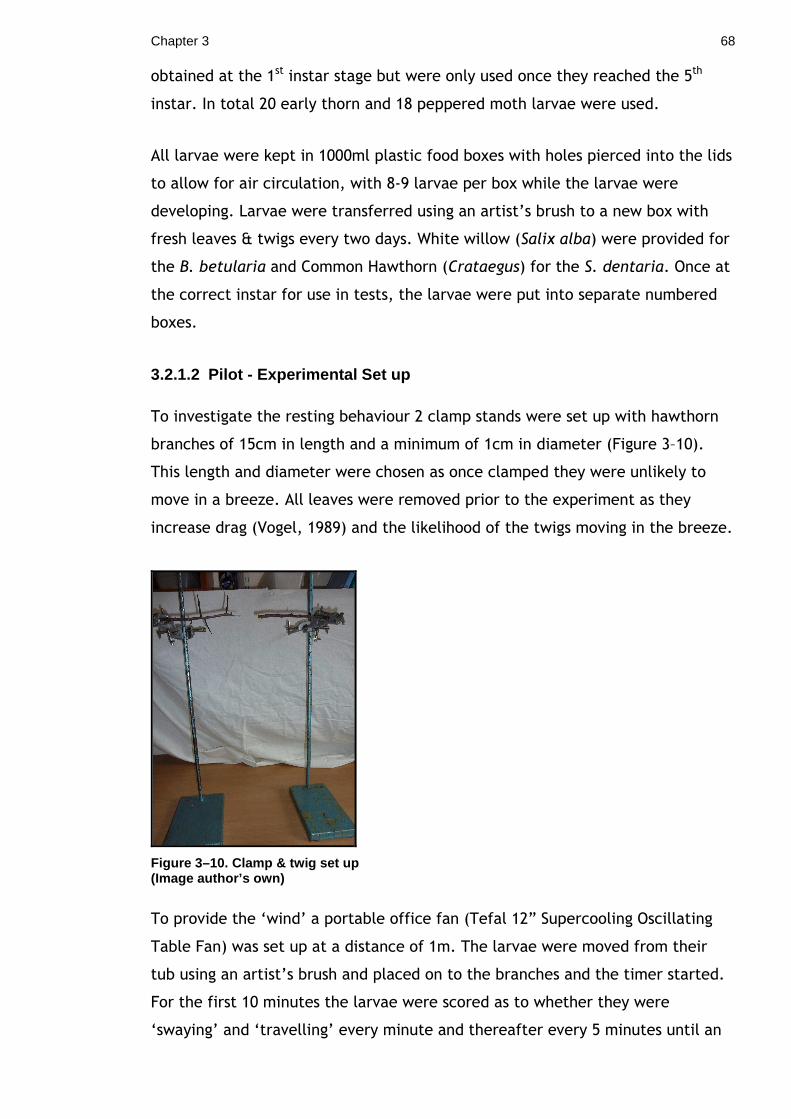
Chapter 3 68
obtained at the 1st instar stage but were only used once they reached the 5th
instar. In total 20 early thorn and 18 peppered moth larvae were used.
All larvae were kept in 1000ml plastic food boxes with holes pierced into the lids
to allow for air circulation, with 8-9 larvae per box while the larvae were
developing. Larvae were transferred using an artist’s brush to a new box with
fresh leaves & twigs every two days. White willow (Salix alba) were provided for
the B. betularia and Common Hawthorn (Crataegus) for the S. dentaria. Once at
the correct instar for use in tests, the larvae were put into separate numbered
boxes.
3.2.1.2 Pilot - Experimental Set up
To investigate the resting behaviour 2 clamp stands were set up with hawthorn
branches of 15cm in length and a minimum of 1cm in diameter (Figure 3–10).
This length and diameter were chosen as once clamped they were unlikely to
move in a breeze. All leaves were removed prior to the experiment as they
increase drag (Vogel, 1989) and the likelihood of the twigs moving in the breeze.
Figure 3–10. Clamp & twig set up (Image author’s own)
To provide the ‘wind’ a portable office fan (Tefal 12” Supercooling Oscillating
Table Fan) was set up at a distance of 1m. The larvae were moved from their
tub using an artist’s brush and placed on to the branches and the timer started.
For the first 10 minutes the larvae were scored as to whether they were
‘swaying’ and ‘travelling’ every minute and thereafter every 5 minutes until an
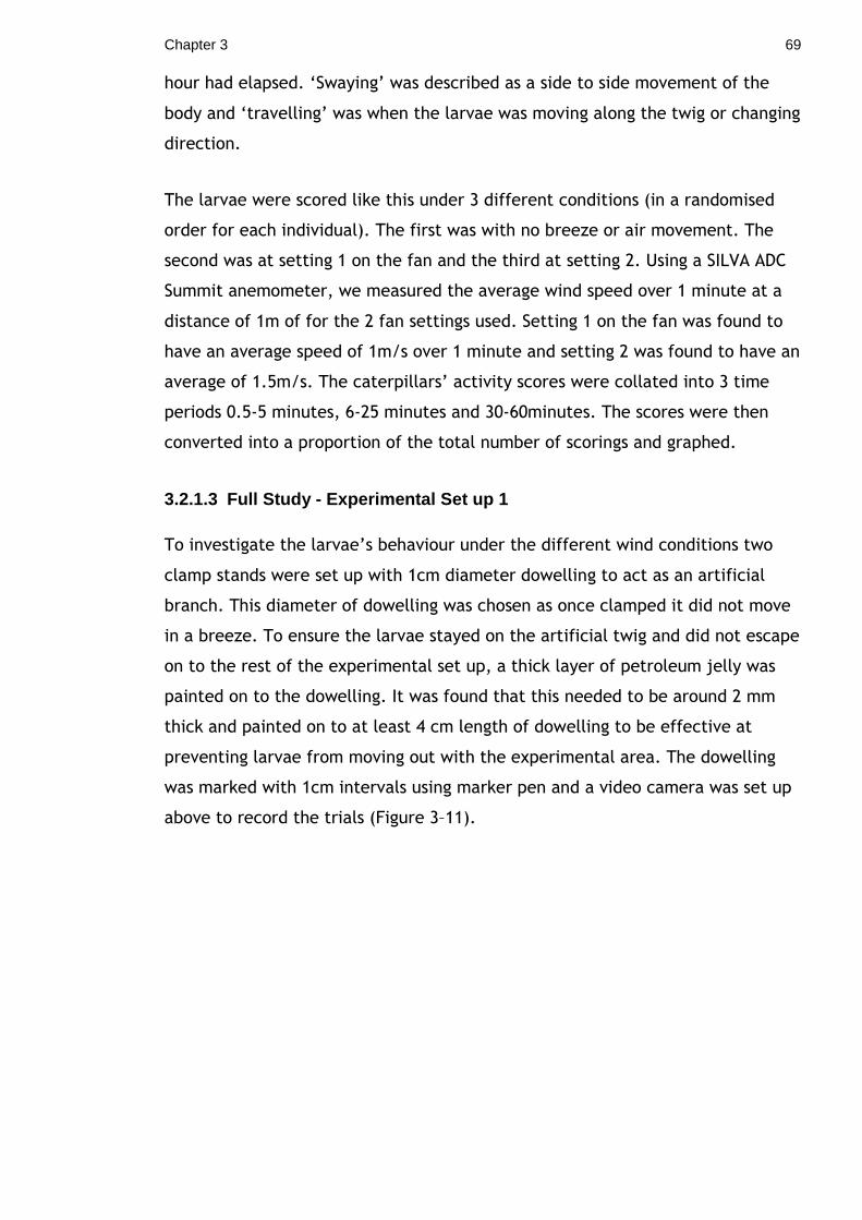
Chapter 3 69
hour had elapsed. ‘Swaying’ was described as a side to side movement of the
body and ‘travelling’ was when the larvae was moving along the twig or changing
direction.
The larvae were scored like this under 3 different conditions (in a randomised
order for each individual). The first was with no breeze or air movement. The
second was at setting 1 on the fan and the third at setting 2. Using a SILVA ADC
Summit anemometer, we measured the average wind speed over 1 minute at a
distance of 1m of for the 2 fan settings used. Setting 1 on the fan was found to
have an average speed of 1m/s over 1 minute and setting 2 was found to have an
average of 1.5m/s. The caterpillars’ activity scores were collated into 3 time
periods 0.5-5 minutes, 6-25 minutes and 30-60minutes. The scores were then
converted into a proportion of the total number of scorings and graphed.
3.2.1.3 Full Study - Experimental Set up 1
To investigate the larvae’s behaviour under the different wind conditions two
clamp stands were set up with 1cm diameter dowelling to act as an artificial
branch. This diameter of dowelling was chosen as once clamped it did not move
in a breeze. To ensure the larvae stayed on the artificial twig and did not escape
on to the rest of the experimental set up, a thick layer of petroleum jelly was
painted on to the dowelling. It was found that this needed to be around 2 mm
thick and painted on to at least 4 cm length of dowelling to be effective at
preventing larvae from moving out with the experimental area. The dowelling
was marked with 1cm intervals using marker pen and a video camera was set up
above to record the trials (Figure 3–11).
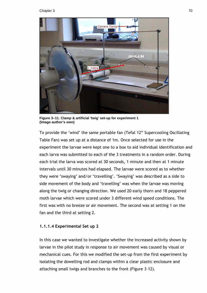
Chapter 3 70
Figure 3–11. Clamp & artificial ‘twig’ set-up for e xperiment 1 (Image author’s own)
To provide the ‘wind’ the same portable fan (Tefal 12” Supercooling Oscillating
Table Fan) was set up at a distance of 1m. Once selected for use in the
experiment the larvae were kept one to a box to aid individual identification and
each larva was submitted to each of the 3 treatments in a random order. During
each trial the larva was scored at 30 seconds, 1 minute and then at 1 minute
intervals until 30 minutes had elapsed. The larvae were scored as to whether
they were ‘swaying’ and/or ‘travelling’. ‘Swaying’ was described as a side to
side movement of the body and ‘travelling’ was when the larvae was moving
along the twig or changing direction. We used 20 early thorn and 18 peppered
moth larvae which were scored under 3 different wind speed conditions. The
first was with no breeze or air movement. The second was at setting 1 on the
fan and the third at setting 2.
1.1.1.4 Experimental Set up 2
In this case we wanted to investigate whether the increased activity shown by
larvae in the pilot study in response to air movement was caused by visual or
mechanical cues. For this we modified the set-up from the first experiment by
isolating the dowelling rod and clamps within a clear plastic enclosure and
attaching small twigs and branches to the front (Figure 3–12).
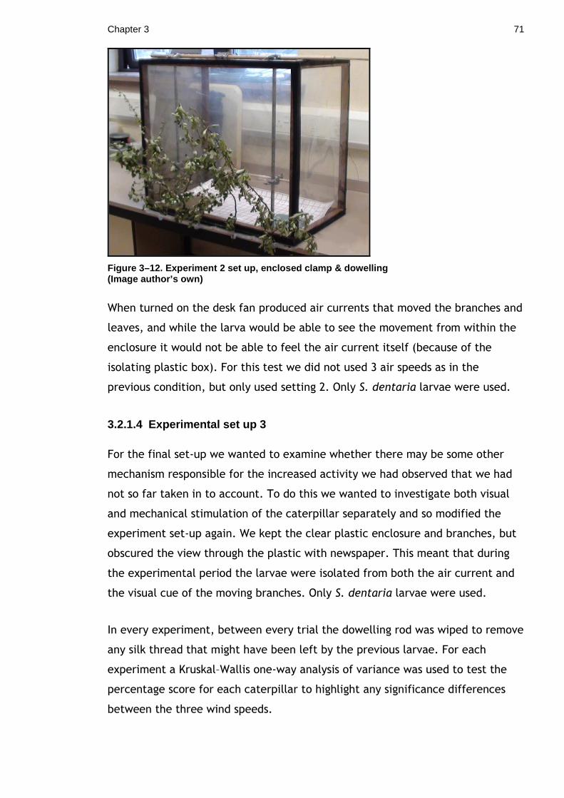
Chapter 3 71
Figure 3–12. Experiment 2 set up, enclosed clamp & dowelling (Image author’s own)
When turned on the desk fan produced air currents that moved the branches and
leaves, and while the larva would be able to see the movement from within the
enclosure it would not be able to feel the air current itself (because of the
isolating plastic box). For this test we did not used 3 air speeds as in the
previous condition, but only used setting 2. Only S. dentaria larvae were used.
3.2.1.4 Experimental set up 3
For the final set-up we wanted to examine whether there may be some other
mechanism responsible for the increased activity we had observed that we had
not so far taken in to account. To do this we wanted to investigate both visual
and mechanical stimulation of the caterpillar separately and so modified the
experiment set-up again. We kept the clear plastic enclosure and branches, but
obscured the view through the plastic with newspaper. This meant that during
the experimental period the larvae were isolated from both the air current and
the visual cue of the moving branches. Only S. dentaria larvae were used.
In every experiment, between every trial the dowelling rod was wiped to remove
any silk thread that might have been left by the previous larvae. For each
experiment a Kruskal–Wallis one-way analysis of variance was used to test the
percentage score for each caterpillar to highlight any significance differences
between the three wind speeds.
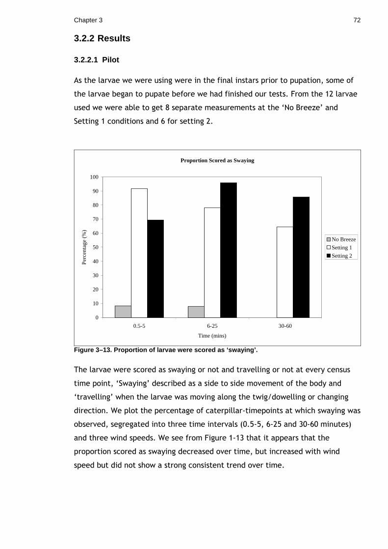
Chapter 3 72
3.2.2 Results
3.2.2.1 Pilot
As the larvae we were using were in the final instars prior to pupation, some of
the larvae began to pupate before we had finished our tests. From the 12 larvae
used we were able to get 8 separate measurements at the ‘No Breeze’ and
Setting 1 conditions and 6 for setting 2.
Proportion Scored as Swaying
0
10
20
30
40
50
60
70
80
90
100
0.5-5 6-25 30-60
Time (mins)
Per
cent
age
(%)
No Breeze
Setting 1
Setting 2
Figure 3–13. Proportion of larvae were scored as ‘s waying’.
The larvae were scored as swaying or not and travelling or not at every census
time point, ‘Swaying’ described as a side to side movement of the body and
‘travelling’ when the larvae was moving along the twig/dowelling or changing
direction. We plot the percentage of caterpillar-timepoints at which swaying was
observed, segregated into three time intervals (0.5-5, 6-25 and 30-60 minutes)
and three wind speeds. We see from Figure 1-13 that it appears that the
proportion scored as swaying decreased over time, but increased with wind
speed but did not show a strong consistent trend over time.
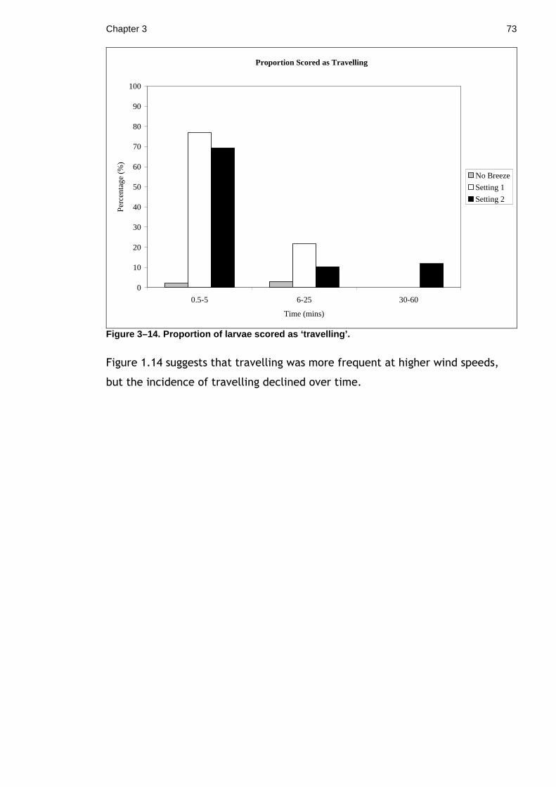
Chapter 3 73
Proportion Scored as Travelling
0
10
20
30
40
50
60
70
80
90
100
0.5-5 6-25 30-60
Time (mins)
Per
cent
age
(%)
No Breeze
Setting 1
Setting 2
Figure 3–14. Proportion of larvae scored as ‘travel ling’.
Figure 1.14 suggests that travelling was more frequent at higher wind speeds,
but the incidence of travelling declined over time.
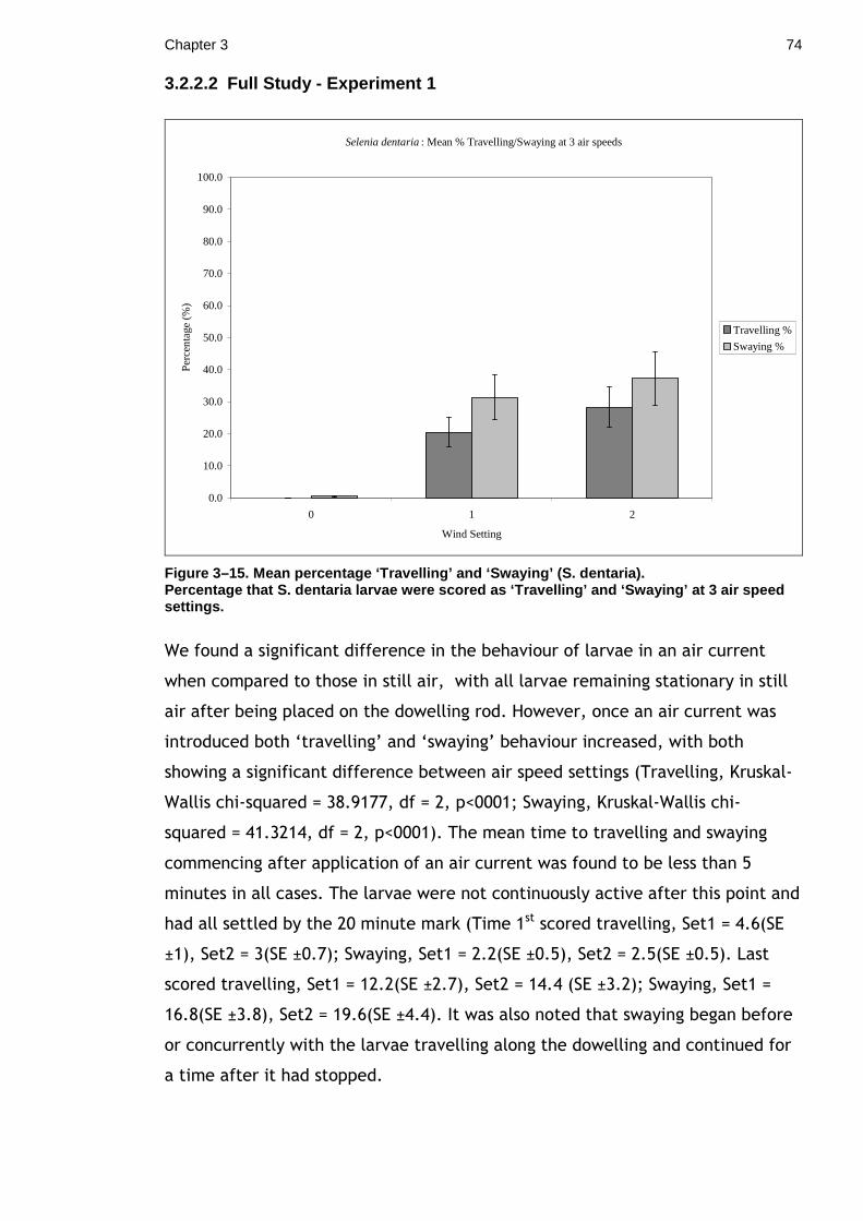
Chapter 3 74
3.2.2.2 Full Study - Experiment 1
Selenia dentaria : Mean % Travelling/Swaying at 3 air speeds
0.0
10.0
20.0
30.0
40.0
50.0
60.0
70.0
80.0
90.0
100.0
0 1 2
Wind Setting
Per
cent
age
(%)
Travelling %
Swaying %
Figure 3–15. Mean percentage ‘Travelling’ and ‘Sway ing’ (S. dentaria). Percentage that S. dentaria larvae were scored as ‘ Travelling’ and ‘Swaying’ at 3 air speed settings.
We found a significant difference in the behaviour of larvae in an air current
when compared to those in still air, with all larvae remaining stationary in still
air after being placed on the dowelling rod. However, once an air current was
introduced both ‘travelling’ and ‘swaying’ behaviour increased, with both
showing a significant difference between air speed settings (Travelling, Kruskal-
Wallis chi-squared = 38.9177, df = 2, p<0001; Swaying, Kruskal-Wallis chi-
squared = 41.3214, df = 2, p<0001). The mean time to travelling and swaying
commencing after application of an air current was found to be less than 5
minutes in all cases. The larvae were not continuously active after this point and
had all settled by the 20 minute mark (Time 1st scored travelling, Set1 = 4.6(SE
±1), Set2 = 3(SE ±0.7); Swaying, Set1 = 2.2(SE ±0.5), Set2 = 2.5(SE ±0.5). Last
scored travelling, Set1 = 12.2(SE ±2.7), Set2 = 14.4 (SE ±3.2); Swaying, Set1 =
16.8(SE ±3.8), Set2 = 19.6(SE ±4.4). It was also noted that swaying began before
or concurrently with the larvae travelling along the dowelling and continued for
a time after it had stopped.
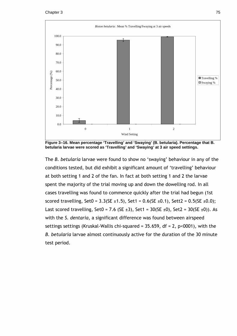
Chapter 3 75
Biston betularia : Mean % Travelling/Swaying at 3 air speeds
0.0
10.0
20.0
30.0
40.0
50.0
60.0
70.0
80.0
90.0
100.0
0 1 2
Wind Setting
Per
cent
age
(%)
Travelling %
Swaying %
Figure 3–16. Mean percentage ‘Travelling’ and ‘Sway ing’ ( B. betularia). Percentage that B. betularia larvae were scored as ‘Travelling’ and ‘Swaying’ a t 3 air speed settings.
The B. betularia larvae were found to show no ‘swaying’ behaviour in any of the
conditions tested, but did exhibit a significant amount of ‘travelling’ behaviour
at both setting 1 and 2 of the fan. In fact at both setting 1 and 2 the larvae
spent the majority of the trial moving up and down the dowelling rod. In all
cases travelling was found to commence quickly after the trial had begun (1st
scored travelling, Set0 = 3.3(SE ±1.5), Set1 = 0.6(SE ±0.1), Sett2 = 0.5(SE ±0.0);
Last scored travelling, Set0 = 7.6 (SE ±3), Set1 = 30(SE ±0), Set2 = 30(SE ±0)). As
with the S. dentaria, a significant difference was found between airspeed
settings settings (Kruskal-Wallis chi-squared = 35.659, df = 2, p<0001), with the
B. betularia larvae almost continuously active for the duration of the 30 minute
test period.
Chapter 3 76
3.2.2.3 Full Study - Experiment 2
When isolated from air currents, but able to view the movement the air
produced in leaves and twigs set up between the fan and enclosure, the S.
dentaria larvae spent 0.3 % (SE ±0.1) of their time travelling compared to 28.2%
(SE±6.3) found without the barrier. Although a small amount of ‘swaying’ was
seen this was very much reduced from the non-isolated condition with 21.4%
(SE±6.18) compared to the previous 37.3 (SE±8.3). Both swaying and travelling
were found to differ significantly between the Isolated condition and the non-
isolated condition (Exp1) (Travelling, Mann-Whitney U = 1, p<0.001; Swaying, U =
21, p<0.001).
3.2.2.4 Full Study - Experiment 3
When isolated from air currents and unable to see the effects of the air currents
the larvae behaved as they did when no air currents were being generated with
very little ‘swaying’ or ‘travelling’ behaviour (% time travelling = 0.3 SE ±0.3;
swaying = 1.6 SE ±1.09).
Both travelling and swaying were found to be significantly different when
compared against the original non-isolated and blinded test (Exp1) (Travelling, U
= 1, p<0.001; Swaying, U = 5, p<0.001).Travelling was not found to be
significantly different between the isolated (Exp2) and the isolated and blinded
larvae (Exp3) (Travelling, U = 72, p = 1). Swaying behaviour was found to be
significantly different (Swaying, U = 37, p<0.001) between the isolated and
isolated and blinded conditions.
3.2.3 Discussion
The results of our first experiment show that, as expected for a species that
relies upon masquerade to reduce predation, under still air conditions S.
dentaria larvae remain very still. However, in conditions that mimic a natural
breeze, the larvae became active moving around the artificial twig before
settling in to the typical resting ‘twig’ like pose before the end of the test
period. Also of note is that the S. dentaria larvae displayed a characteristic side
to side swaying movement which began either concurrently with or just before
the larvae began to move along the artificial twig. We do however have to
Chapter 3 77
consider the possibility that the swaying is not generated by the larvae
themselves. As described in the methods section we took a number of
precautions to ensure that the twigs in the pilot study and the dowelling rod in
the main study remained still throughout the experiment and so we feel
confident that movement is not being transferred in this way. Further, the
larvae stopped swaying when they eventually settled on a fixed position on the
substrate. The air currents the larvae were tested in are the equivalent of 1 on
the Beaufort Scale (light air) and considerable lower than what might be
expected on an average British summer’s day, making it unlikely that the larvae
were forced to move due to discomfort caused by the strength of the air
current. This suggests some sort of adaptive behaviour particularly as early thorn
larvae are twig mimics for which movement against a still background
potentially introduces a greater risk of discovery (Ioannou and Krause 2009).
The behaviour we have described may be evidence that S. dentaria uses the
visually confusing movement of leaves and branches moving around in windy
conditions to camouflage their movement. Seen in other cryptic and mimetic
species such as leaf mimics and stick insects (Edmunds and Brunner, 1999;
Robinson, 1966) the swaying movement is thought to be a form of cryptic
movement designed to blend in with background movement of leaves and
branches. What we propose is that by moving in windy conditions and using a
swaying-like movement to mimic the movement of background vegetation larvae
are able to move between foraging locations without incurring the costs we
would normally associate with a cryptic or masquerading species being active
during daylight hours. The fact that the caterpillars eventually stopped swaying
when they stopped moving suggests that this behaviour acts to reduced dangers
associated with movement on their host-plant, rather than being a more
generalised mimicking of visual movement in the background.
Of course if an increase in background noise can increase crypsis it also has
implications for species that use visual signals for intra-species communication
and some recent studies have suggested this. For example some lizard species
that use body movements for territorial displays and signalling, have been found
to modify their signalling movements in response to increased vegetation
movement in windy conditions (Ord et al., 2007; Peters et al., 2007). Similarly,
insects that use vibrations to signal potential mates have been found to
Chapter 3 78
predominately signal in still wind conditions and are less successful in the
presence of wind induced vibrations (McNett et al., 2010). These results strongly
suggest that wind can adversely affect detection not only by unintended
recipients (such as predators) but by intended targets.
When we then tested B. betularia under the same conditions it was found that
while both S. dentaria and B. betularia remained still in the still air conditions,
B. betula was considerably more active than S. dentaria in the ‘windy’
conditions and did not show any ‘swaying’ behaviour. In fact the B. betula larvae
we tested spent almost the entirety of the trial periods walking up and down the
artificial twig. It is difficult to say why this difference should exist as both
species are typical twig mimics, with both strongly resembling the inedible twigs
of their host plant species. It may be possible that differences in host tree
species flexibility, leaf shape and branch distribution may produce considerable
differences in their movement in windy conditions. Theses differences are likely
to change the effectiveness of cryptic movement and other anti-predator
strategies. It may also be possible that the slightly larger body size of B.
betularia in comparison to S. dentaria makes holding the typical ‘twig’ pose
more difficult in more open and wind blown positions, but this seems unlikely
when the air currents we used in this test were well below the average wind
strength you might expect over a British summer. Finally, it may be that B.
betularia is pickier in their selection of resting site and while the air currents
were available to camouflage their movement they are unwilling to settle until a
more suitable site than the artificial twig we provided.
In the second and third experiments we conducted we wanted to investigate
whether the larvae were using physical or visual cues to determine when to use
the cryptic movement strategy. The travelling and swaying scores from the
experiments in which the larvae were either isolated from the air movement by
a perspex sheet (Exp2) or isolated and blinded to the visual effects of the sir
currents, differed significantly from the equivalent wind speed setting for the
non-isolated or blinded first experiments (Exp1). When compared against each
other the isolated and isolated and blinded results, not significantly different
from each other for travelling, did differ for the swaying results, with the
isolated individuals only showing greater swaying than the isolated and blinded
tests.
Chapter 3 79
Our results suggest that the larvae are most likely using mechanical stimulation
from air currents passing over their body as a physical cue to conditions, rather
than visual or other cues to determine air conditions. The cues are therefore
most likely from air currents disturbing hairs and bristles on the larvae’s body
surface. However, the percentage swaying scores for Experiment 2 where the
larvae were isolated from air currents but able to see their effects on leaves and
twigs outside the enclosure, were considerably greater than expected. This may
indicate that perhaps the swaying behaviour has some visual component to it.
However, when examined further it was noted that the majority of the
unexpected result came from 1 outlier (larva 8) and if this one data point is
removed the results become considerably closer to what we saw in the isolated
and blinded experiment.
It is also possible that the slight increase in travelling and swaying seen in the
isolated conditions when compared to the still air conditions may be due to our
experimental set-up not perfectly sheltering the larvae from all the air
movement generated. In both experiments it was noted that small air
movements were still evident near the top opening of the enclosure and from
some corner joints. While very small it is possible that this was detected by the
larvae and may in fact explain a problem we had with larvae repeatedly
dropping off the twig. This behaviour is consistent with dropping as an anti-
predator behaviour noted in other lepidopteran species. In this instance small air
vibrations from the wings of predatory insects such as bees or wasps can cause
larvae to freeze and drop off their host plant (Tautz, 1978; Tautz and Markl,
1978; Tautz and Rostás, 2008).
A useful development from our study might be to examine the effect on
predation rate of being cryptic and remaining stationary against a moving
background. In Ioannou and Krause’s 2009 paper they found that remaining
motionless was an important component in preventing detection in cryptic
organism, but their study was carried out against a static background. It would
be interesting to see if there was a corresponding cost to remaining still when
against a moving background. For instance if you are a twig or leaf mimic in
windy conditions, but do not mimic the movement are you more easily spotted?
We suggest that this could be tested with the use of video or computer graphics
which either have a static or swaying stimuli in front of a moving background of
Chapter 3 80
vegetation. To test for a difference in survival human volunteers (or birds
trained to peck a screen, (Dittrich et al., 2010; Taylor et al., 2002) could be
timed to see how quickly and accurately they can pick out the different stimuli.
In conclusion our results suggest that twig-mimicking lepidopteran species may
be using wind generated movement of the leaves and twigs of their host plants
to camouflage their own movements. There is also evidence that in some cases
larvae may utilise specialised ‘swaying’ movements to further camouflage their
movements. As cryptic species are generally limited in their opportunities to
move between sites due to the increased risk of detection by predators, any
adaptation that reduces predation while allowing movement between foraging
sites could be extremely advantageous.
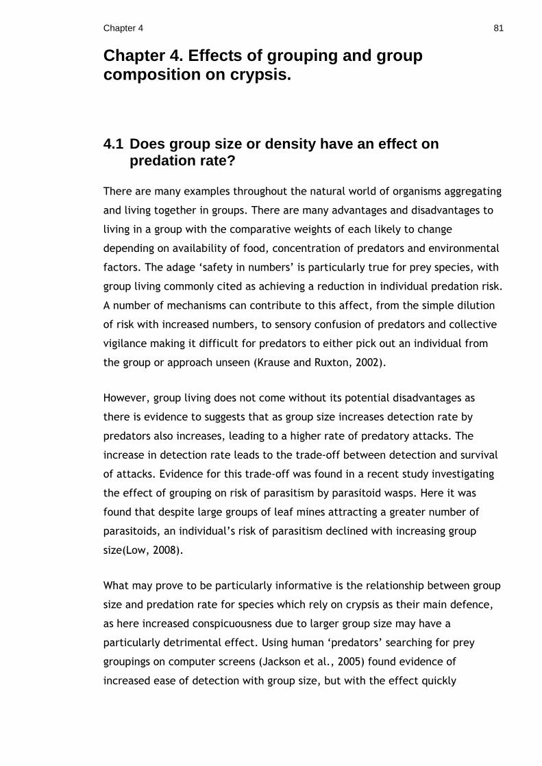
Chapter 4 81
Chapter 4. Effects of grouping and group composition on crypsis.
4.1 Does group size or density have an effect on predation rate?
There are many examples throughout the natural world of organisms aggregating
and living together in groups. There are many advantages and disadvantages to
living in a group with the comparative weights of each likely to change
depending on availability of food, concentration of predators and environmental
factors. The adage ‘safety in numbers’ is particularly true for prey species, with
group living commonly cited as achieving a reduction in individual predation risk.
A number of mechanisms can contribute to this affect, from the simple dilution
of risk with increased numbers, to sensory confusion of predators and collective
vigilance making it difficult for predators to either pick out an individual from
the group or approach unseen (Krause and Ruxton, 2002).
However, group living does not come without its potential disadvantages as
there is evidence to suggests that as group size increases detection rate by
predators also increases, leading to a higher rate of predatory attacks. The
increase in detection rate leads to the trade-off between detection and survival
of attacks. Evidence for this trade-off was found in a recent study investigating
the effect of grouping on risk of parasitism by parasitoid wasps. Here it was
found that despite large groups of leaf mines attracting a greater number of
parasitoids, an individual’s risk of parasitism declined with increasing group
size(Low, 2008).
What may prove to be particularly informative is the relationship between group
size and predation rate for species which rely on crypsis as their main defence,
as here increased conspicuousness due to larger group size may have a
particularly detrimental effect. Using human ‘predators’ searching for prey
groupings on computer screens (Jackson et al., 2005) found evidence of
increased ease of detection with group size, but with the effect quickly
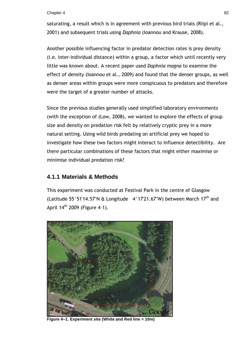
Chapter 4 82
saturating, a result which is in agreement with previous bird trials (Riipi et al.,
2001) and subsequent trials using Daphnia (Ioannou and Krause, 2008).
Another possible influencing factor in predator detection rates is prey density
(i.e. inter-individual distance) within a group, a factor which until recently very
little was known about. A recent paper used Daphnia magna to examine the
effect of density (Ioannou et al., 2009) and found that the denser groups, as well
as denser areas within groups were more conspicuous to predators and therefore
were the target of a greater number of attacks.
Since the previous studies generally used simplified laboratory environments
(with the exception of (Low, 2008), we wanted to explore the effects of group
size and density on predation risk felt by relatively cryptic prey in a more
natural setting. Using wild birds predating on artificial prey we hoped to
investigate how these two factors might interact to influence detectibility. Are
there particular combinations of these factors that might either maximise or
minimise individual predation risk?
4.1.1 Materials & Methods
This experiment was conducted at Festival Park in the centre of Glasgow
(Latitude 55°51'14.57"N & Longitude 4°17'21.67"W) between March 17th and
April 14th 2009 (Figure 4–1).
Figure 4–1. Experiment site (White and Red line = 1 0m)

Chapter 4 83
Each trial took place over 1 hour with 18 different treatments per trial and a
total of 45 trials over the experimental period. The treatments consisted of
either Black or Striped sunflower seeds in group sizes of 5, 15, or 30 seeds
spread over an area of 4cm, 10cm or 20cm diameter (Figure 4–2) for example
groups). To ensure that the seeds from each group were spread over the desired
area circular cardboard ‘stencils’ cut to the correct diameters were used.
Figure 4–2. Example seed groups. 30 striped sunflower seed groups spread over 10cm d iameter (Left) and 4cm (Right) diameter areas. (Image Author’s own)
The 18 treatments were set out in a different randomly generated order each
day and assayed for predation 1 hour later in the same order. The groups were
set out with a minimum of 10m between them and after the experimental period
had elapsed the remaining seeds from each treatment were counted and totals
recorded. To ensure the remaining seeds were found quickly on return to the
site, markers (golf tees) were placed 2m from each group. In order to more
easily and quickly find the seed groups a stick was placed at the edge of the
seed group and a golf tee placed at the other end (Figure 4–3). Once the stick is
removed we believe the tee was sufficiently distant from the seed group as to
prevent it being used as a cue. When retrieving the seeds the coloured golf tee
is more easily found than the seeds and when placed next to the tee the stick
points directly at the seed group.
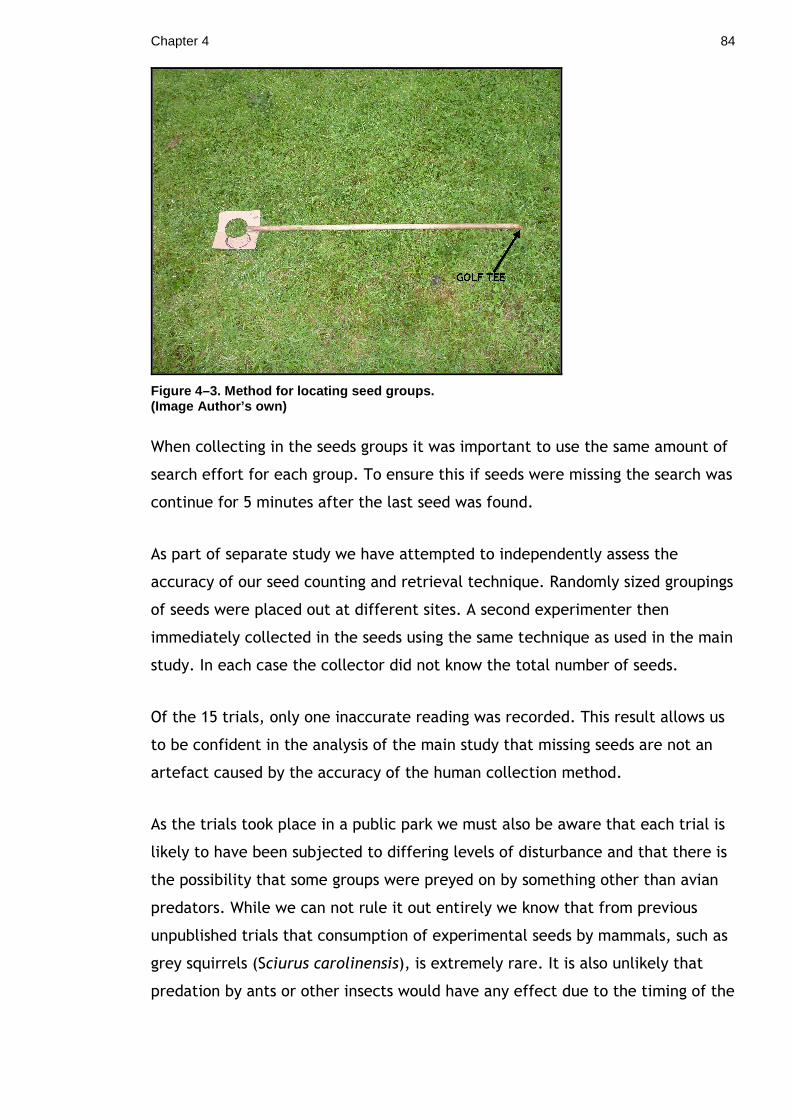
Chapter 4 84
Figure 4–3. Method for locating seed groups. (Image Author’s own)
When collecting in the seeds groups it was important to use the same amount of
search effort for each group. To ensure this if seeds were missing the search was
continue for 5 minutes after the last seed was found.
As part of separate study we have attempted to independently assess the
accuracy of our seed counting and retrieval technique. Randomly sized groupings
of seeds were placed out at different sites. A second experimenter then
immediately collected in the seeds using the same technique as used in the main
study. In each case the collector did not know the total number of seeds.
Of the 15 trials, only one inaccurate reading was recorded. This result allows us
to be confident in the analysis of the main study that missing seeds are not an
artefact caused by the accuracy of the human collection method.
As the trials took place in a public park we must also be aware that each trial is
likely to have been subjected to differing levels of disturbance and that there is
the possibility that some groups were preyed on by something other than avian
predators. While we can not rule it out entirely we know that from previous
unpublished trials that consumption of experimental seeds by mammals, such as
grey squirrels (Sciurus carolinensis), is extremely rare. It is also unlikely that
predation by ants or other insects would have any effect due to the timing of the

Chapter 4 85
trials in early spring and by having the test period during the day we minimised
the likelihood of rodent predation.
The data recorded for each trial included the date, the time at which the
treatments were placed out and collected in and the time at which the site was
left. The temperature and weather conditions for Glasgow were recorded for
9am and 12pm from the MET office website
(http://www.metoffice.gov.uk/education/archive/uk/).
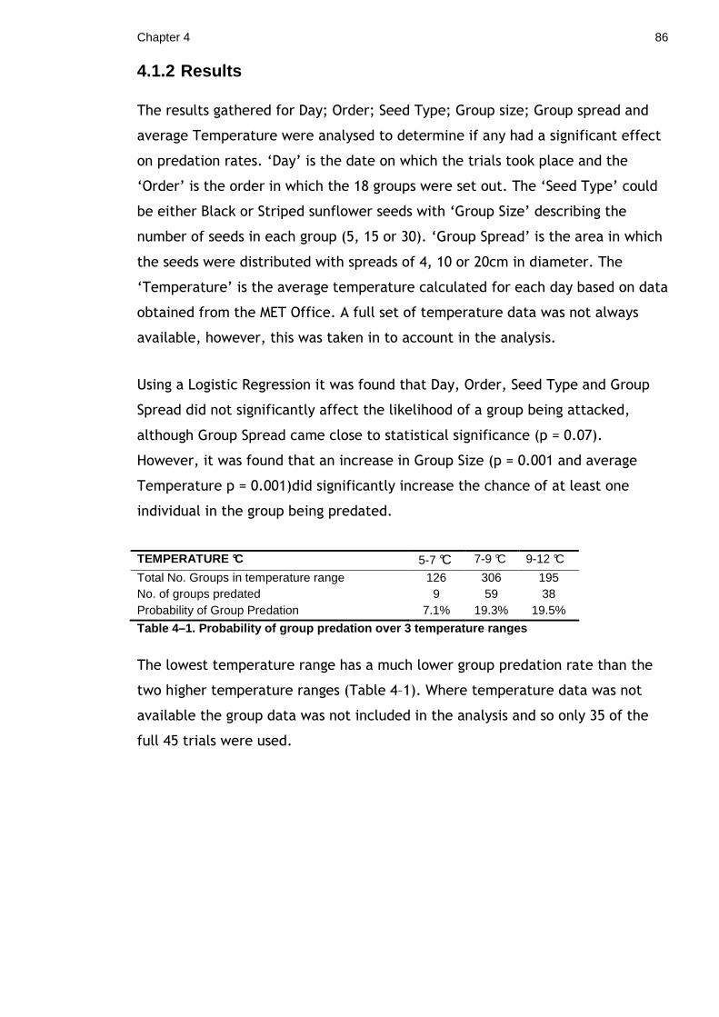
Chapter 4 86
4.1.2 Results
The results gathered for Day; Order; Seed Type; Group size; Group spread and
average Temperature were analysed to determine if any had a significant effect
on predation rates. ‘Day’ is the date on which the trials took place and the
‘Order’ is the order in which the 18 groups were set out. The ‘Seed Type’ could
be either Black or Striped sunflower seeds with ‘Group Size’ describing the
number of seeds in each group (5, 15 or 30). ‘Group Spread’ is the area in which
the seeds were distributed with spreads of 4, 10 or 20cm in diameter. The
‘Temperature’ is the average temperature calculated for each day based on data
obtained from the MET Office. A full set of temperature data was not always
available, however, this was taken in to account in the analysis.
Using a Logistic Regression it was found that Day, Order, Seed Type and Group
Spread did not significantly affect the likelihood of a group being attacked,
although Group Spread came close to statistical significance (p = 0.07).
However, it was found that an increase in Group Size (p = 0.001 and average
Temperature p = 0.001)did significantly increase the chance of at least one
individual in the group being predated.
TEMPERATURE °C 5-7 °C 7-9 °C 9-12 °C
Total No. Groups in temperature range 126 306 195 No. of groups predated 9 59 38 Probability of Group Predation 7.1% 19.3% 19.5%
Table 4–1. Probability of group predation over 3 te mperature ranges
The lowest temperature range has a much lower group predation rate than the
two higher temperature ranges (Table 4–1). Where temperature data was not
available the group data was not included in the analysis and so only 35 of the
full 45 trials were used.
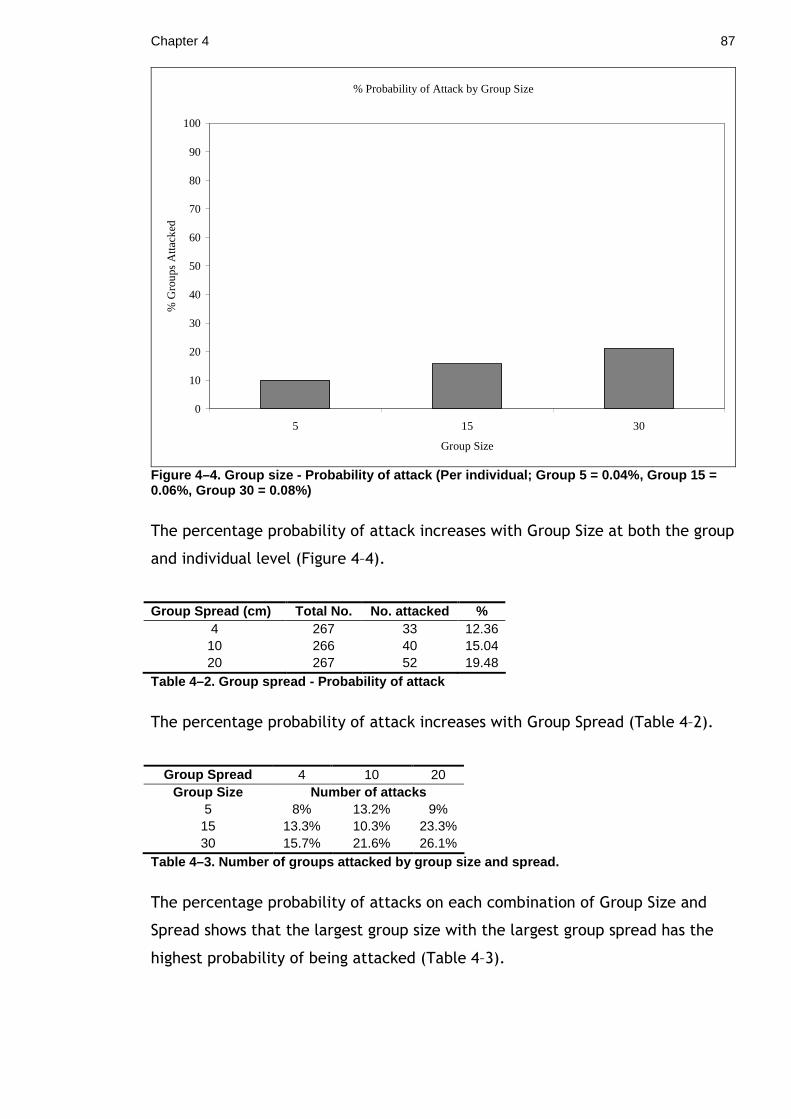
Chapter 4 87
% Probability of Attack by Group Size
0
10
20
30
40
50
60
70
80
90
100
5 15 30
Group Size
% G
roup
s A
ttack
ed
Figure 4–4. Group size - Probability of attack (Per individual; Group 5 = 0.04%, Group 15 = 0.06%, Group 30 = 0.08%)
The percentage probability of attack increases with Group Size at both the group
and individual level (Figure 4–4).
Group Spread (cm) Total No. No. attacked % 4 267 33 12.36 10 266 40 15.04 20 267 52 19.48
Table 4–2. Group spread - Probability of attack
The percentage probability of attack increases with Group Spread (Table 4–2).
Group Spread 4 10 20 Group Size Number of attacks
5 8% 13.2% 9% 15 13.3% 10.3% 23.3% 30 15.7% 21.6% 26.1%
Table 4–3. Number of groups attacked by group size and spread.
The percentage probability of attacks on each combination of Group Size and
Spread shows that the largest group size with the largest group spread has the
highest probability of being attacked (Table 4–3).
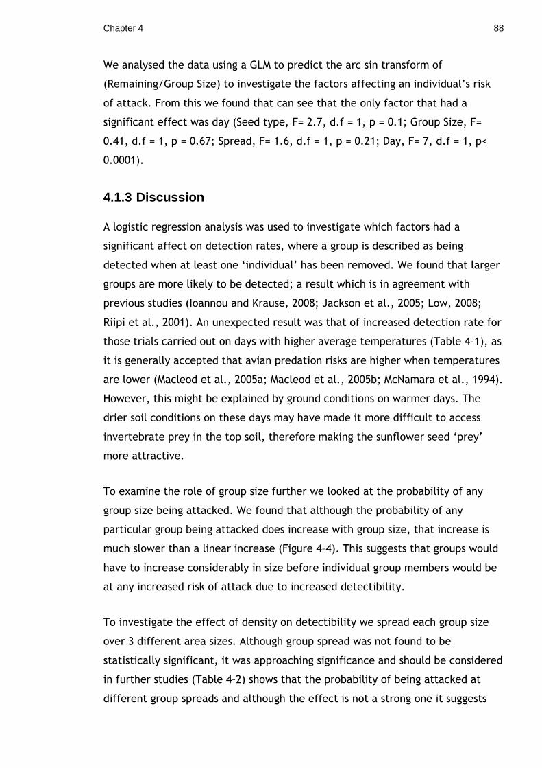
Chapter 4 88
We analysed the data using a GLM to predict the arc sin transform of
(Remaining/Group Size) to investigate the factors affecting an individual’s risk
of attack. From this we found that can see that the only factor that had a
significant effect was day (Seed type, F= 2.7, d.f = 1, p = 0.1; Group Size, F=
0.41, d.f = 1, p = 0.67; Spread, F= 1.6, d.f = 1, p = 0.21; Day, F= 7, d.f = 1, p<
0.0001).
4.1.3 Discussion
A logistic regression analysis was used to investigate which factors had a
significant affect on detection rates, where a group is described as being
detected when at least one ‘individual’ has been removed. We found that larger
groups are more likely to be detected; a result which is in agreement with
previous studies (Ioannou and Krause, 2008; Jackson et al., 2005; Low, 2008;
Riipi et al., 2001). An unexpected result was that of increased detection rate for
those trials carried out on days with higher average temperatures (Table 4–1), as
it is generally accepted that avian predation risks are higher when temperatures
are lower (Macleod et al., 2005a; Macleod et al., 2005b; McNamara et al., 1994).
However, this might be explained by ground conditions on warmer days. The
drier soil conditions on these days may have made it more difficult to access
invertebrate prey in the top soil, therefore making the sunflower seed ‘prey’
more attractive.
To examine the role of group size further we looked at the probability of any
group size being attacked. We found that although the probability of any
particular group being attacked does increase with group size, that increase is
much slower than a linear increase (Figure 4–4). This suggests that groups would
have to increase considerably in size before individual group members would be
at any increased risk of attack due to increased detectibility.
To investigate the effect of density on detectibility we spread each group size
over 3 different area sizes. Although group spread was not found to be
statistically significant, it was approaching significance and should be considered
in further studies (Table 4–2) shows that the probability of being attacked at
different group spreads and although the effect is not a strong one it suggests
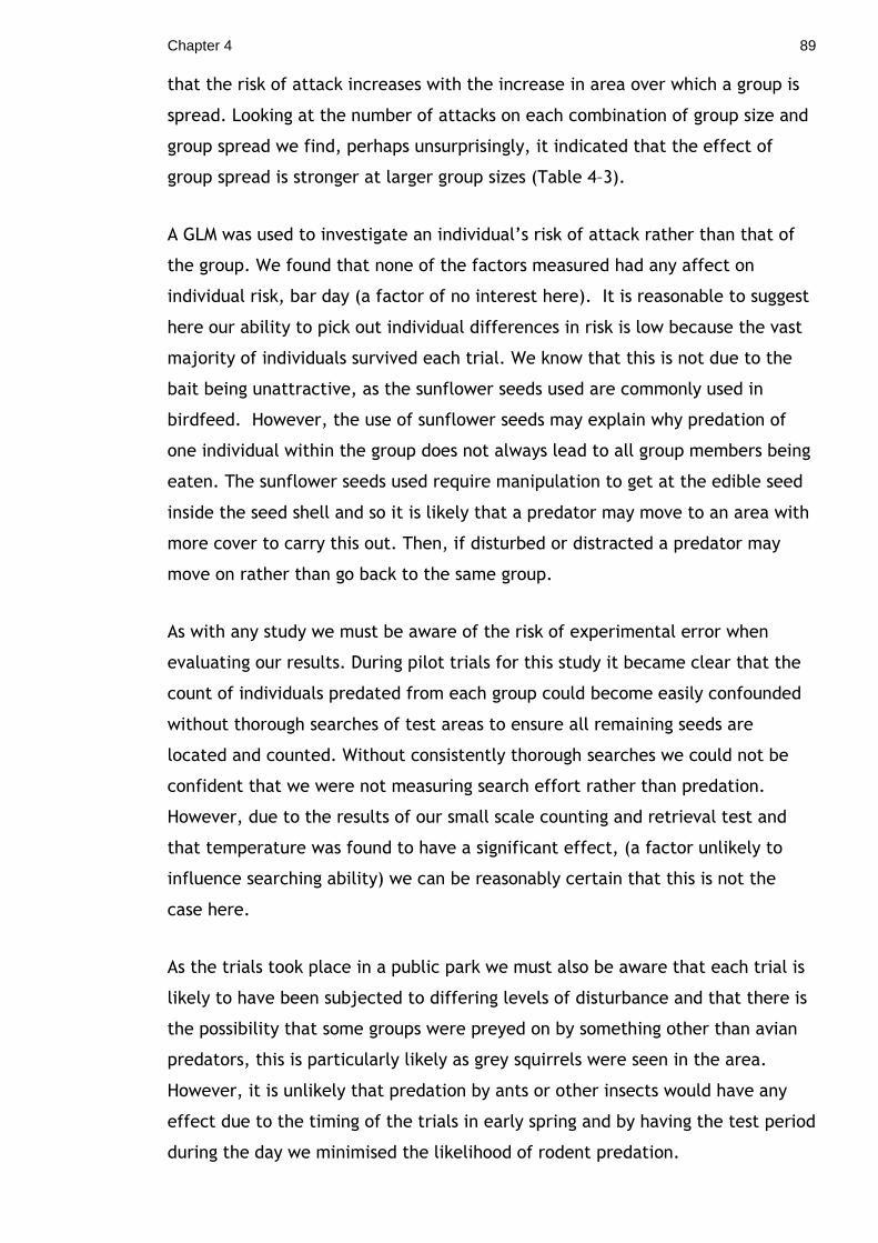
Chapter 4 89
that the risk of attack increases with the increase in area over which a group is
spread. Looking at the number of attacks on each combination of group size and
group spread we find, perhaps unsurprisingly, it indicated that the effect of
group spread is stronger at larger group sizes (Table 4–3).
A GLM was used to investigate an individual’s risk of attack rather than that of
the group. We found that none of the factors measured had any affect on
individual risk, bar day (a factor of no interest here). It is reasonable to suggest
here our ability to pick out individual differences in risk is low because the vast
majority of individuals survived each trial. We know that this is not due to the
bait being unattractive, as the sunflower seeds used are commonly used in
birdfeed. However, the use of sunflower seeds may explain why predation of
one individual within the group does not always lead to all group members being
eaten. The sunflower seeds used require manipulation to get at the edible seed
inside the seed shell and so it is likely that a predator may move to an area with
more cover to carry this out. Then, if disturbed or distracted a predator may
move on rather than go back to the same group.
As with any study we must be aware of the risk of experimental error when
evaluating our results. During pilot trials for this study it became clear that the
count of individuals predated from each group could become easily confounded
without thorough searches of test areas to ensure all remaining seeds are
located and counted. Without consistently thorough searches we could not be
confident that we were not measuring search effort rather than predation.
However, due to the results of our small scale counting and retrieval test and
that temperature was found to have a significant effect, (a factor unlikely to
influence searching ability) we can be reasonably certain that this is not the
case here.
As the trials took place in a public park we must also be aware that each trial is
likely to have been subjected to differing levels of disturbance and that there is
the possibility that some groups were preyed on by something other than avian
predators, this is particularly likely as grey squirrels were seen in the area.
However, it is unlikely that predation by ants or other insects would have any
effect due to the timing of the trials in early spring and by having the test period
during the day we minimised the likelihood of rodent predation.
Chapter 4 90
Future studies of group size and density would greatly benefit from a much
larger sample size, particularly if we want to be able to see the effects at an
individual level. Another possible avenue of investigation is suggested by the
fact that there appeared to be no predator preference shown to either the
striped or black sunflower seeds used. We have taken this idea further by using
them in mixed groups and manipulating the proportion of each seed type and
using them to investigate whether there is any effect of prey ‘oddity’ on
predator preference (See Chapter 4).
Chapter 4 91
4.2 Field test of the effect of ‘oddity’ within a g roup on predation risk.
It is well known that prey species form groups to defend themselves from
predator attack, with group members benefiting from the accumulation of many
different anti-predator mechanisms(Krause and Ruxton, 2002). The ‘confusion
effect’ is a well-documented phenomenon found across a wide range of
predatory taxa (Jeschke and Tollrian, 2007), which effectively reduces a
predator’s attack to kill ratio. It does this by limiting their ability to single out
and successfully attack one individual within a group, with the effect further
enhanced with visually similar prey (Krakauer, 1995; Tosh et al., 2006).
The effectiveness of grouping at reducing predation has led to speculation as to
how predators might overcome this problem. A well documented candidate is
the ‘oddity effect’. This hypothesises that when confronted by grouped prey
predators can increase their kill rate by concentrating their efforts on capturing
unusual or ‘odd’ prey. These ‘odd’ prey types stand out of the crowd with the
effect of reducing or potentially overcoming the ‘confusion effect’ entirely
(Landeau and Terborgh, 1986; Ohguchi, 1978). While this is an attractive idea,
and one which has historically been used to explain cases where rare or ‘odd’
individuals appear to have been preferentially targeted, there have been
comparatively few studies which have been able to conclusively demonstrate
this effect. There are also possible confounding issues to be looked at such as
whether ‘odd’ individuals are in fact just more highly sought after prey items, or
whether they are more conspicuous within the environment regardless of other
group members. There may also be other complicating factors such as
differences in defence capabilities (Mathis and Chivers, 2003) and prey density
(Allen et al., 1998) both of which have been shown to modify prey selection.
An often-cited study of the oddity effect is that of Landeau & Terborgh (1986)
where the interactions of largemouth bass (Micropterus salmoides) and groups of
silvery minnows (Hybognathus nuchalis) were used. They were able to show that
by including one or two ‘odd’ individuals in a group of 8 prey successful capture
of both the odd and normal prey was greatly increased, and that this effect
disappeared as the number of ‘odd’ individuals was increased to 50%. There was
also the suggestion that the oddity effect may be confined to small group sizes,
Chapter 4 92
but more recent studies have not been able to find any evidence to support this
(Krakauer, 1995; Ruxton et al., 2007). However, they were able to confirm that
the oddity effect disappeared as the ‘odd’ phenotype increased to 50%(Ruxton
et al., 2007).
Another well known and related concept is that of apostatic selection where
predators show a preference for the more common prey type (Endler, 1991) with
anti-apostatic selection describing a preference for rare morphs. From this we
can see that the description given for anti-apostatic selection is very similar to
that of the oddity effect. The main differences are those of scale: with apostatic
selection generally considered at population level and the oddity effect within
smaller groupings where prey are viewed simultaneously by predators. Further
reasoning for this separation is that the oddity effect is generally invoked as a
method of mediating the effects of the confusion effect, an effect generally
assumed to require aggregations of moving prey. However, Krakauer’s (1995)
paper which is often cited as theoretical evidence for the confusion effect,
found evidence of both the confusion and oddity effects within a static prey
system. We would therefore like to expand upon this and investigate whether
predators of slow moving or sedentary prey aggregations might be benefiting
from the oddity effect.
Recent studies investigating the diversity of fish assemblages inhabiting coral
reefs have provided support for the idea that predators may reduce species
diversity within a system by targeting rare species (Almany et al., 2006; Almany
and Webster, 2004). In these cases it was found that although not more
vulnerable to predators due to appearance or colouration, rare prey species
suffered consistently greater predation. Work investigating prey choices in wild
bird populations has found that they switch prey types in response to changes in
morph frequency to maintain anti-apostatic selection (Allen and Weale, 2005).
These studies suggest that anti-apostatic selection and the oddity effect are
mechanisms by which predators can be strong influences on diversity at both the
species and community level and provide credence to those proposing that
frequency-dependent selection such as apostatic selection or the oddity effect
may be a major force driving evolution with the power to cause the divergence
or convergence of phenotypic traits(Greenwood, 1985). There are also
potentially important implications for rare prey species conservation as there
Chapter 4 93
may be a tipping point at which predators will switch prey preferences to
already dwindling populations.
It is for these reasons we feel that it is important to investigate and understand
the circumstances under which anti-apostatic selection and/or oddity effects
occur. We propose to use wild birds as our predator assemblage, as to our
knowledge no previous study exploring the effect of oddity has used wild-living
predators. We have elected to use groups of inert prey in the form of either
black or striped sunflowers seeds to avoid any confounding factors generated by
within-group interactions between mobile prey. Previous studies within the
experimental area have found that the resident wild bird population does not
show a preference when presented with same-sized groups of each morph. This
provides us with the opportunity to use mixed groups to look for any effect of
oddity. We hope to answer 3 questions:
1) Do ‘odd’ individuals within a group suffer greater predation risk than their
‘normal’ group mates?
2) Does the presence of ‘odd’ individuals increase the predation risk of other
individuals within the group?
3) Is there any evidence for the oddity effect in groups of stationary prey?
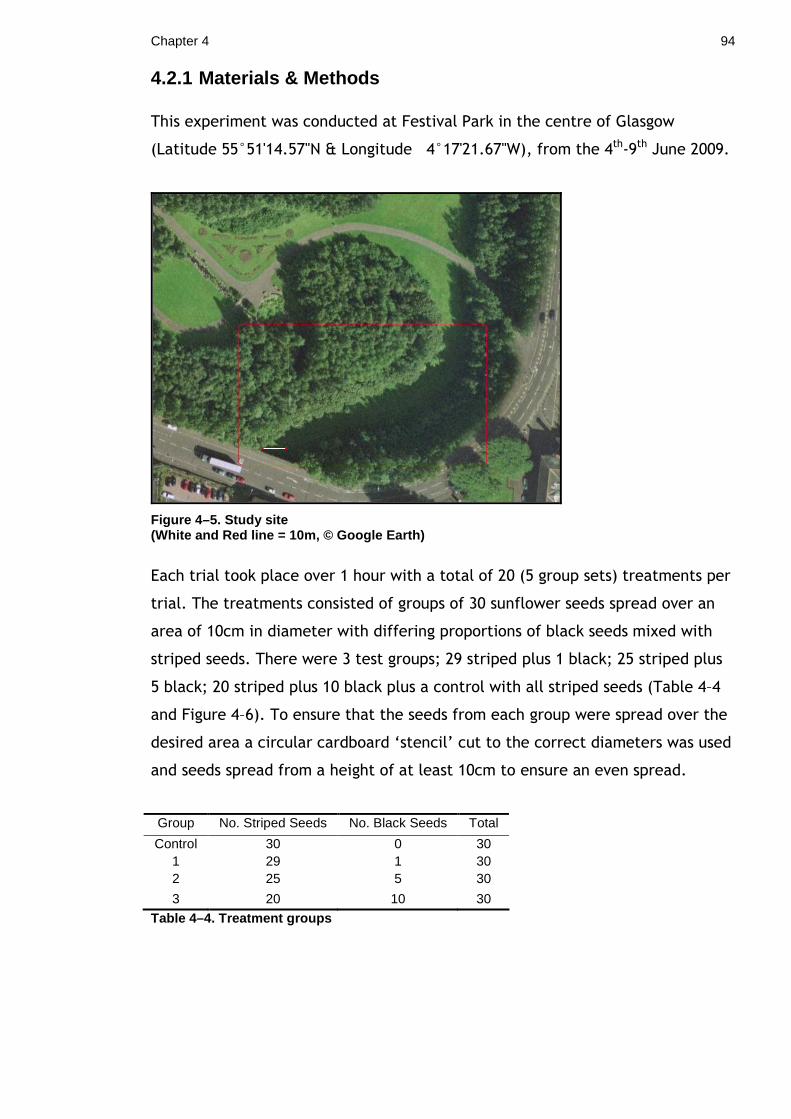
Chapter 4 94
4.2.1 Materials & Methods
This experiment was conducted at Festival Park in the centre of Glasgow
(Latitude 55°51'14.57"N & Longitude 4°17'21.67"W), from the 4th-9th June 2009.
Figure 4–5. Study site (White and Red line = 10m, © Google Earth)
Each trial took place over 1 hour with a total of 20 (5 group sets) treatments per
trial. The treatments consisted of groups of 30 sunflower seeds spread over an
area of 10cm in diameter with differing proportions of black seeds mixed with
striped seeds. There were 3 test groups; 29 striped plus 1 black; 25 striped plus
5 black; 20 striped plus 10 black plus a control with all striped seeds (Table 4–4
and Figure 4–6). To ensure that the seeds from each group were spread over the
desired area a circular cardboard ‘stencil’ cut to the correct diameters was used
and seeds spread from a height of at least 10cm to ensure an even spread.
Group No. Striped Seeds No. Black Seeds Total
Control 30 0 30 1 29 1 30 2 25 5 30
3 20 10 30
Table 4–4. Treatment groups
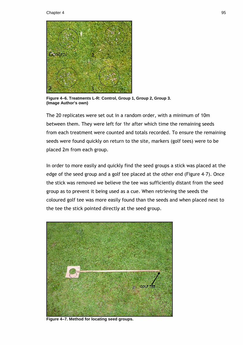
Chapter 4 95
Figure 4–6. Treatments L-R: Control, Group 1, Group 2, Group 3. (Image Author’s own)
The 20 replicates were set out in a random order, with a minimum of 10m
between them. They were left for 1hr after which time the remaining seeds
from each treatment were counted and totals recorded. To ensure the remaining
seeds were found quickly on return to the site, markers (golf tees) were to be
placed 2m from each group.
In order to more easily and quickly find the seed groups a stick was placed at the
edge of the seed group and a golf tee placed at the other end (Figure 4–7). Once
the stick was removed we believe the tee was sufficiently distant from the seed
group as to prevent it being used as a cue. When retrieving the seeds the
coloured golf tee was more easily found than the seeds and when placed next to
the tee the stick pointed directly at the seed group.
Figure 4–7. Method for locating seed groups.
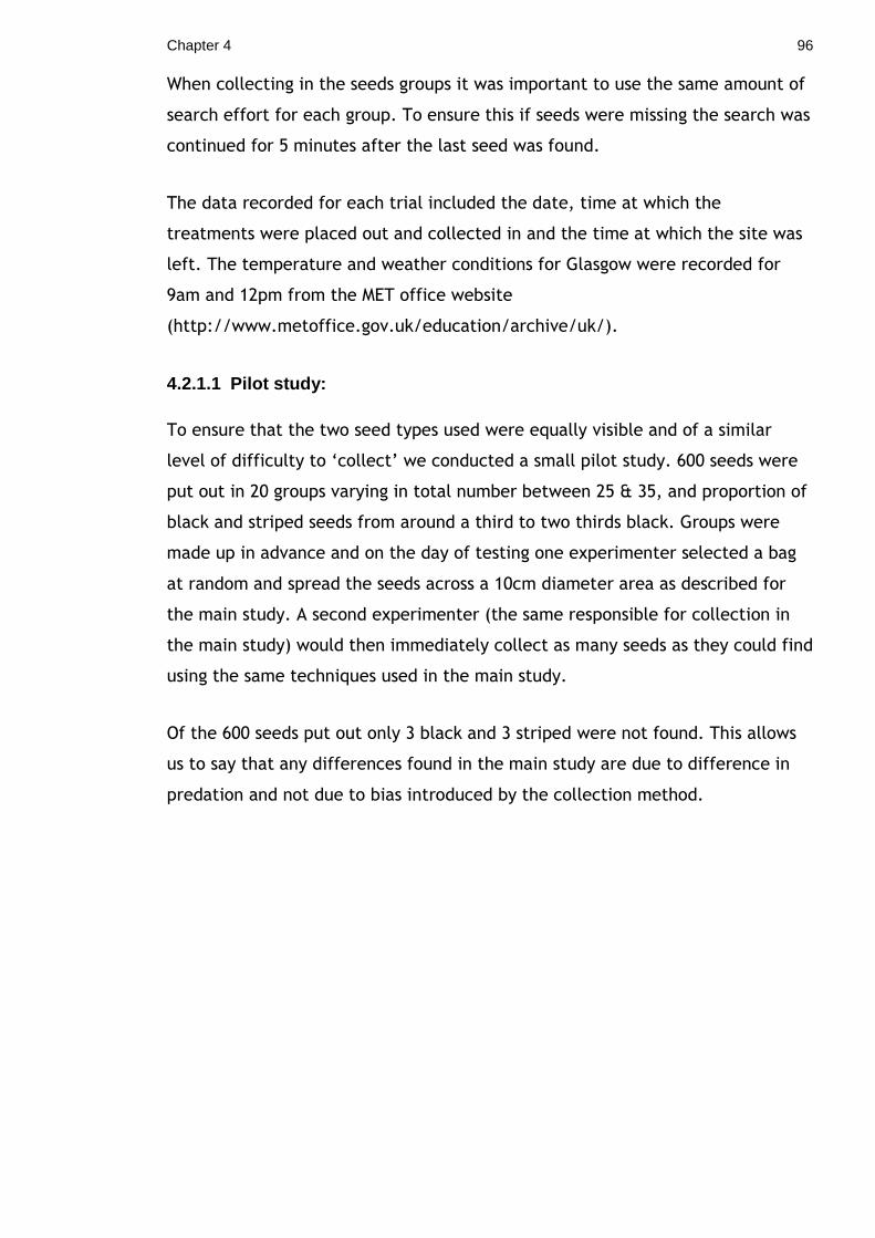
Chapter 4 96
When collecting in the seeds groups it was important to use the same amount of
search effort for each group. To ensure this if seeds were missing the search was
continued for 5 minutes after the last seed was found.
The data recorded for each trial included the date, time at which the
treatments were placed out and collected in and the time at which the site was
left. The temperature and weather conditions for Glasgow were recorded for
9am and 12pm from the MET office website
(http://www.metoffice.gov.uk/education/archive/uk/).
4.2.1.1 Pilot study:
To ensure that the two seed types used were equally visible and of a similar
level of difficulty to ‘collect’ we conducted a small pilot study. 600 seeds were
put out in 20 groups varying in total number between 25 & 35, and proportion of
black and striped seeds from around a third to two thirds black. Groups were
made up in advance and on the day of testing one experimenter selected a bag
at random and spread the seeds across a 10cm diameter area as described for
the main study. A second experimenter (the same responsible for collection in
the main study) would then immediately collect as many seeds as they could find
using the same techniques used in the main study.
Of the 600 seeds put out only 3 black and 3 striped were not found. This allows
us to say that any differences found in the main study are due to difference in
predation and not due to bias introduced by the collection method.
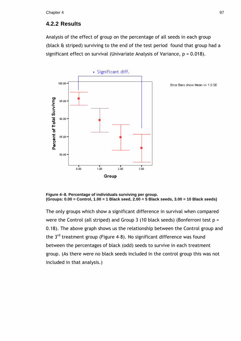
Chapter 4 97
4.2.2 Results
Analysis of the effect of group on the percentage of all seeds in each group
(black & striped) surviving to the end of the test period found that group had a
significant effect on survival (Univariate Analysis of Variance, p = 0.018).
Figure 4–8. Percentage of individuals surviving per group. (Groups: 0.00 = Control, 1.00 = 1 Black seed, 2.00 = 5 Black seeds, 3.00 = 10 Black seeds)
The only groups which show a significant difference in survival when compared
were the Control (all striped) and Group 3 (10 black seeds) (Bonferroni test p =
0.18). The above graph shows us the relationship between the Control group and
the 3rd treatment group (Figure 4–8). No significant difference was found
between the percentages of black (odd) seeds to survive in each treatment
group. (As there were no black seeds included in the control group this was not
included in that analysis.)
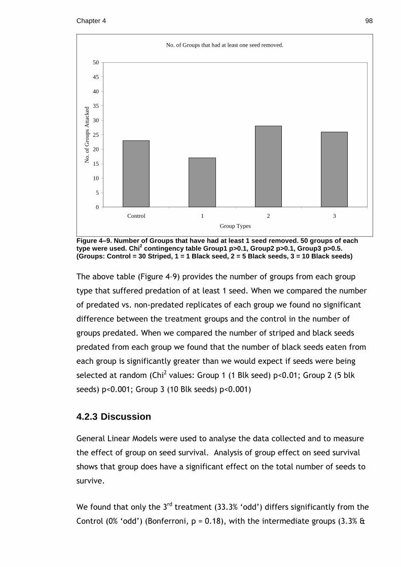
Chapter 4 98
No. of Groups that had at least one seed removed.
0
5
10
15
20
25
30
35
40
45
50
Control 1 2 3
Group Types
No.
of
Gro
ups
Atta
cked
Figure 4–9. Number of Groups that have had at least 1 seed removed. 50 groups of each type were used. Chi 2 contingency table Group1 p>0.1, Group2 p>0.1, Grou p3 p>0.5. (Groups: Control = 30 Striped, 1 = 1 Black seed, 2 = 5 Black seeds, 3 = 10 Black seeds)
The above table (Figure 4–9) provides the number of groups from each group
type that suffered predation of at least 1 seed. When we compared the number
of predated vs. non-predated replicates of each group we found no significant
difference between the treatment groups and the control in the number of
groups predated. When we compared the number of striped and black seeds
predated from each group we found that the number of black seeds eaten from
each group is significantly greater than we would expect if seeds were being
selected at random (Chi2 values: Group 1 (1 Blk seed) p<0.01; Group 2 (5 blk
seeds) p<0.001; Group 3 (10 Blk seeds) p<0.001)
4.2.3 Discussion
General Linear Models were used to analyse the data collected and to measure
the effect of group on seed survival. Analysis of group effect on seed survival
shows that group does have a significant effect on the total number of seeds to
survive.
We found that only the 3rd treatment (33.3% ‘odd’) differs significantly from the
Control (0% ‘odd’) (Bonferroni, p = 0.18), with the intermediate groups (3.3% &

Chapter 4 99
16.6% ‘odd’) having no significant effect seed survival to the end of the trial.
This result tells us that seeds in the 3rd treatment group had a significantly
greater chance of being predated.
A previous investigation carried out by Landeau & Terborgh (1986) has found
that groups with 1 or 2 ‘odd’ (12.5-25%) individuals in a group of 8 suffered
greater risk, but when this was increased to 3 or 4 (37.5-50%) the effect
disappeared. A subsequent study by Ruxton et al (2007) has confirmed this upper
limit of 50%. This combined with our results may suggest that there may be a
range where ‘odd’ individuals will increase the predation risk of individuals with
a group.
We examined how group affected the predation of ‘odd’ (black) seeds and found
that there was no significant difference between groups. This suggests that
although groups with more ‘odd’ individuals may suffer greater predation the
risk, the predation rate felt by ‘odd’ individuals is not influenced by the number
of other ‘odd’ individuals in their group.
From our analysis we can be reasonably sure that treatment did not have any
effect on the number of groups that suffered predation (Figure 4–9). This
suggests that the presence of odd individuals does not have any effect on a
group’s overall risk of predation, but does influence the way that risk is
distributed between group members.
We then wanted to investigate whether predators showed any preference for
‘odd’ or ‘normal’ seeds. After analysis we were able to show that ‘odd’ seeds
were removed at a rate greater than would be expected for random prey
selection. This suggests that they are either more conspicuous against the
substrate or in some way preferable and being actively selected. However, a
previous study (unpublished Group experiment) using groups of either all black
(‘odd’) or all striped (‘normal’) seeds found no difference in predation rates
between the groups, suggesting that it is the group composition and their
position within it that is driving the increase in predation risk.
Great care was taken to ensure that all seeds remaining after the trial period
were located and counted. Despite this it is not possible to say that no seeds
Chapter 4 100
were missed. This however, would only be problematic if we believed that one
seed type was more likely to be missed than the other and from the results of
the pilot study carried out we can be reasonably sure that there was no bias in
collection towards either black or striped seeds.
In summary, although the presence of ‘odd’ individuals does not change the
group predation risk (how likely the group is to be attacked) as a whole (1) ‘odd’
prey suffer a greater rate of predation than ‘normal’ conspecifics within the
same group. This effect is not altered by the number of other ‘odd’ prey within
that group. However, (2) the greater the number of ‘odd’ prey within a group
the greater the predation risk felt by all individuals within the group (increased
number removed from the group). Our results also suggest that (3) there is
evidence of the oddity effect within this system despite using static prey, an
observation which concurs with the previous theoretical work carried out by
Krakauer (1995).
What we now need to consider is the reason for birds using this strategy with
stationary prey. When confronted with a group of moving prey it makes sense
that predators need to be able to quickly single out one individual for a
successful attack, but with stationary prey it would seem that there should not
be the same problems. The experimental area used in this study was within a
public park and therefore subject to pedestrian traffic. It is likely that this
limited the length of feeding bouts. Therefore, what we might be seeing here is
the predator using the oddity effect to speed up prey selection which will allow
them to minimise the time spent in the open and/or devote greater attention to
scanning for predators. A recent paper by T. Waite (2008) has suggested that
predators may use a ‘unique choice heuristic’. He proposed that by using a
general rule of thumb where odd prey items are given automatic preference,
predators can skip the deliberating phase of the choice process thereby leaving
more time to scan for danger.
What we need to examine next is the effect of time/predation pressure and how
this affects prey choice and the oddity effect. Further to this it would be
interesting to examine factors other than visual oddity or other aspects of visual
oddity such as prey movement. There has for instance been some indication that
having a different pace or gait may generate the oddity effect (Hatle et al.,
Chapter 4 101
2002) and it may be interesting to look at whether non-visual predators take use
the oddity effect with sound or smell. Examples might be found where there are
groups which share a common scent. Overall there is still much that we need to
look at with regards to the oddity effect, its ecological consequences and
implications for the maintenance of multiple colour morphs within a population.
Chapter 4 102
4.3 Computer based test of the effect of ‘oddity’ w ithin a group on predation risk.
This experiment continues on from our previous study of the oddity effect where
we looked to see if there was any evidence for the oddity effect when predators
are faced with groups of stationary prey. Our results suggested that predators
may be using the oddity effect to select prey. Therefore, we now need to
consider why predators might use this strategy with stationary prey. When
confronted with a group of moving prey it makes sense that predators need to be
able to quickly single out one individual for a successful attack, but with
stationary prey there would appear to be ample time to pick out and consume as
many prey as wanted.
However, this view does not take in to account the risk the predator may face
from its own predators. Therefore, what we may be seeing is a predator using
the oddity effect to speed up prey selection, which then allows them to
minimise the time spent in the open and/or to devote greater attention to
scanning for predators. A recent paper by T. Waite (2008) in which he tested
blue jays (Cyanocitta cristata) for their preference for oddity suggested that
predators may use a ‘unique choice heuristic’. He proposed that by using a
general rule of thumb, where odd prey items are given automatic preference,
predators can skip the deliberating phase of the choice process thereby leaving
more time to scan for danger. Although Waite’s experiment did not use cryptic
prey we might expect to be able to see evidence of this.
For that reason what we wanted to examine in this study is the effect of
time/predation pressure and how this affects prey choice and the oddity effect
when searching for cryptic prey in static groups. Can preference for oddity be
explained by the need to divide attention between multiple tasks?
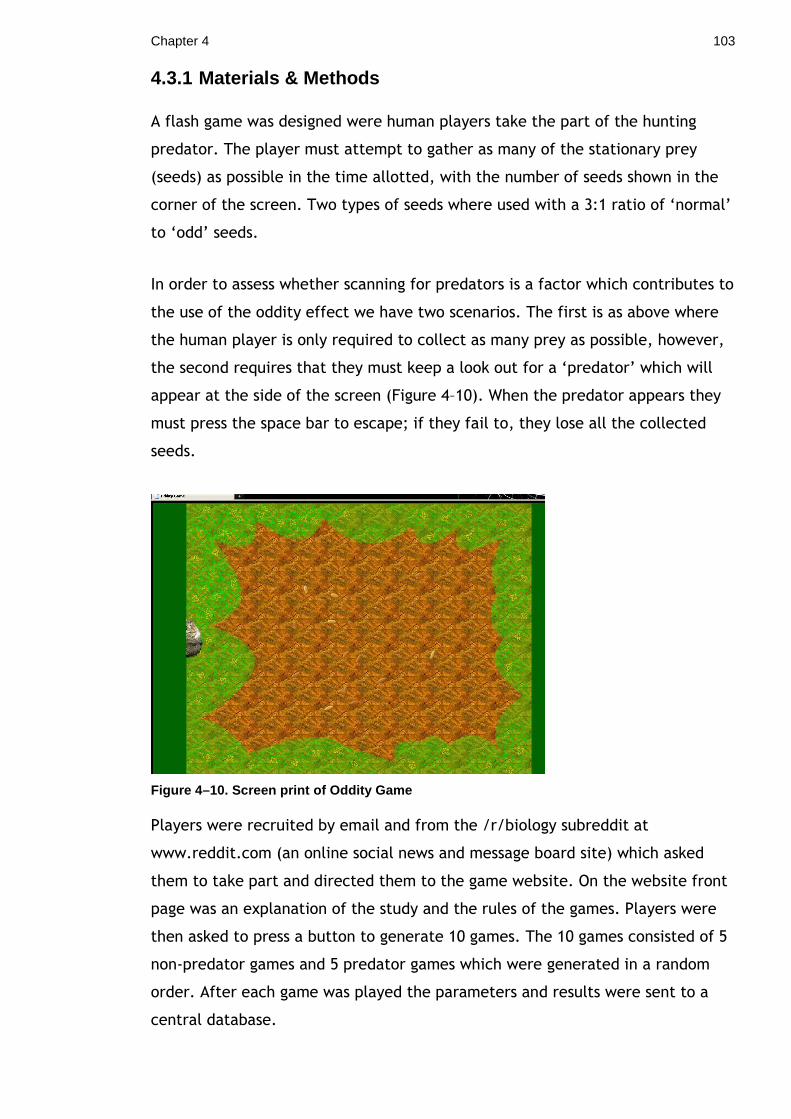
Chapter 4 103
4.3.1 Materials & Methods
A flash game was designed were human players take the part of the hunting
predator. The player must attempt to gather as many of the stationary prey
(seeds) as possible in the time allotted, with the number of seeds shown in the
corner of the screen. Two types of seeds where used with a 3:1 ratio of ‘normal’
to ‘odd’ seeds.
In order to assess whether scanning for predators is a factor which contributes to
the use of the oddity effect we have two scenarios. The first is as above where
the human player is only required to collect as many prey as possible, however,
the second requires that they must keep a look out for a ‘predator’ which will
appear at the side of the screen (Figure 4–10). When the predator appears they
must press the space bar to escape; if they fail to, they lose all the collected
seeds.
Figure 4–10. Screen print of Oddity Game Players were recruited by email and from the /r/biology subreddit at
www.reddit.com (an online social news and message board site) which asked
them to take part and directed them to the game website. On the website front
page was an explanation of the study and the rules of the games. Players were
then asked to press a button to generate 10 games. The 10 games consisted of 5
non-predator games and 5 predator games which were generated in a random
order. After each game was played the parameters and results were sent to a
central database.
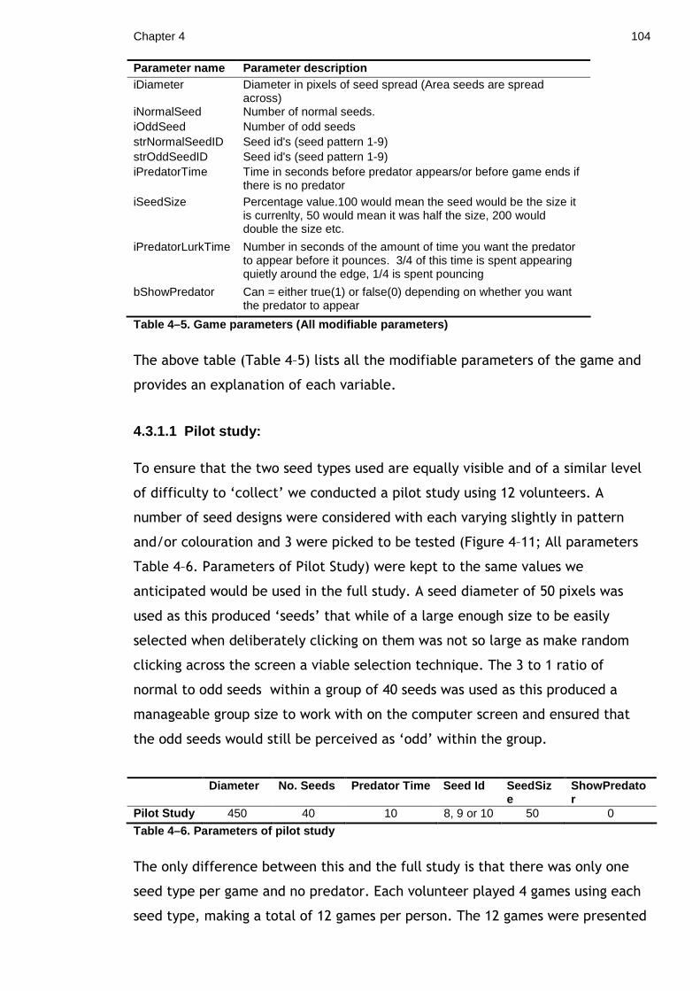
Chapter 4 104
Parameter name Parameter description iDiameter Diameter in pixels of seed spread (Area seeds are spread
across) iNormalSeed Number of normal seeds. iOddSeed Number of odd seeds strNormalSeedID Seed id's (seed pattern 1-9) strOddSeedID Seed id's (seed pattern 1-9) iPredatorTime Time in seconds before predator appears/or before game ends if
there is no predator iSeedSize Percentage value.100 would mean the seed would be the size it
is currenlty, 50 would mean it was half the size, 200 would double the size etc.
iPredatorLurkTime Number in seconds of the amount of time you want the predator to appear before it pounces. 3/4 of this time is spent appearing quietly around the edge, 1/4 is spent pouncing
bShowPredator Can = either true(1) or false(0) depending on whether you want the predator to appear
Table 4–5. Game parameters (All modifiable paramete rs)
The above table (Table 4–5) lists all the modifiable parameters of the game and
provides an explanation of each variable.
4.3.1.1 Pilot study:
To ensure that the two seed types used are equally visible and of a similar level
of difficulty to ‘collect’ we conducted a pilot study using 12 volunteers. A
number of seed designs were considered with each varying slightly in pattern
and/or colouration and 3 were picked to be tested (Figure 4–11; All parameters
Table 4–6. Parameters of Pilot Study) were kept to the same values we
anticipated would be used in the full study. A seed diameter of 50 pixels was
used as this produced ‘seeds’ that while of a large enough size to be easily
selected when deliberately clicking on them was not so large as make random
clicking across the screen a viable selection technique. The 3 to 1 ratio of
normal to odd seeds within a group of 40 seeds was used as this produced a
manageable group size to work with on the computer screen and ensured that
the odd seeds would still be perceived as ‘odd’ within the group.
Diameter No. Seeds Predator Time Seed Id SeedSize
ShowPredator
Pilot Study 450 40 10 8, 9 or 10 50 0
Table 4–6. Parameters of pilot study
The only difference between this and the full study is that there was only one
seed type per game and no predator. Each volunteer played 4 games using each
seed type, making a total of 12 games per person. The 12 games were presented
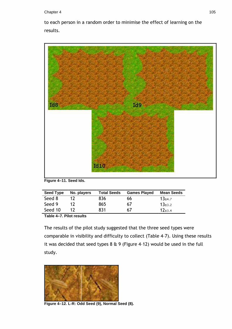
Chapter 4 105
to each person in a random order to minimise the effect of learning on the
results.
Figure 4–11. Seed Ids.
Seed Type No. players Total Seeds Games Played Mea n Seeds
Seed 8 12 836 66 13±4.7 Seed 9 12 865 67 13±3.2 Seed 10 12 831 67 12±3.4 Table 4–7. Pilot results
The results of the pilot study suggested that the three seed types were
comparable in visibility and difficulty to collect (Table 4–7). Using these results
it was decided that seed types 8 & 9 (Figure 4–12) would be used in the full
study.
Figure 4–12. L-R: Odd Seed (9), Normal Seed (8).
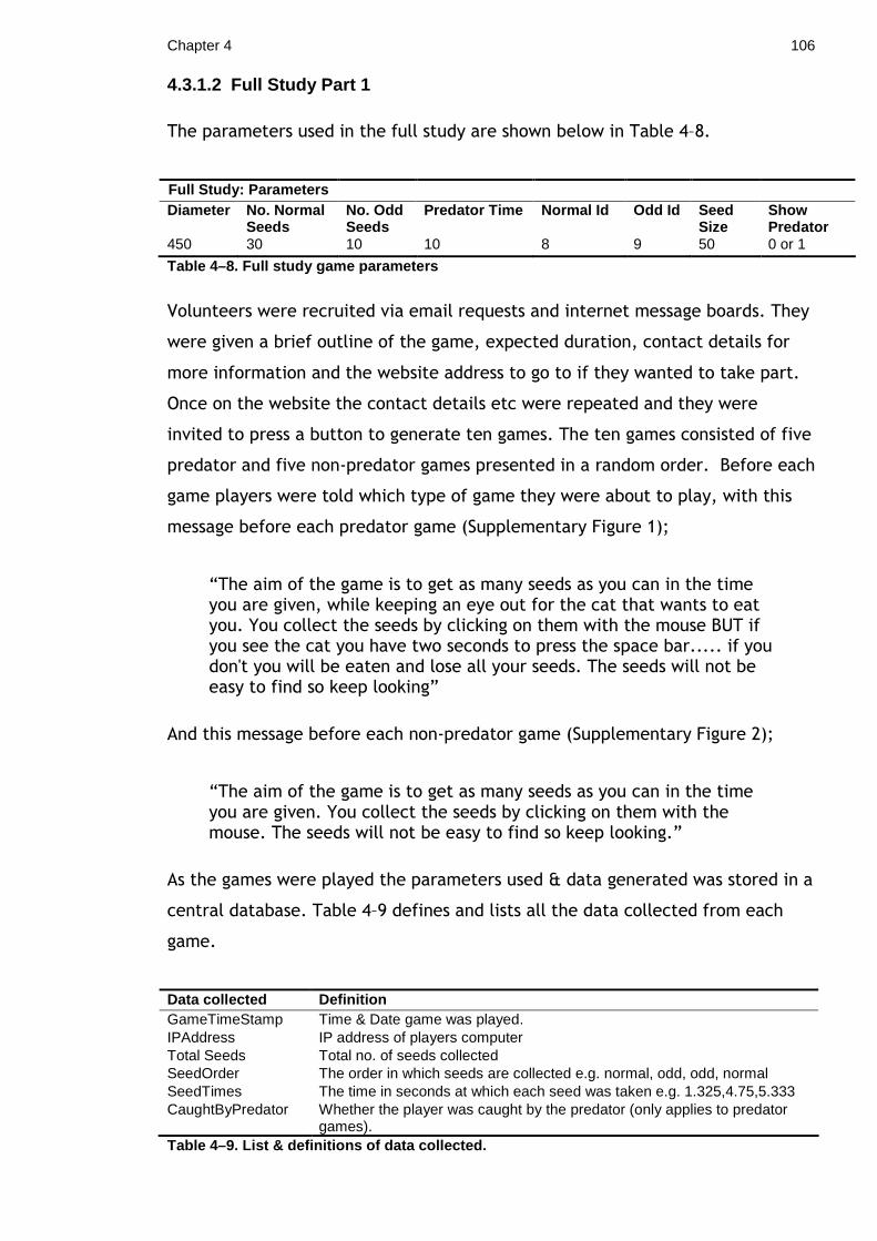
Chapter 4 106
4.3.1.2 Full Study Part 1
The parameters used in the full study are shown below in Table 4–8.
Full Study: Parameters Diameter No. Normal
Seeds No. Odd Seeds
Predator Time Normal Id Odd Id Seed Size
Show Predator
450 30 10 10 8 9 50 0 or 1
Table 4–8. Full study game parameters
Volunteers were recruited via email requests and internet message boards. They
were given a brief outline of the game, expected duration, contact details for
more information and the website address to go to if they wanted to take part.
Once on the website the contact details etc were repeated and they were
invited to press a button to generate ten games. The ten games consisted of five
predator and five non-predator games presented in a random order. Before each
game players were told which type of game they were about to play, with this
message before each predator game (Supplementary Figure 1);
“The aim of the game is to get as many seeds as you can in the time you are given, while keeping an eye out for the cat that wants to eat you. You collect the seeds by clicking on them with the mouse BUT if you see the cat you have two seconds to press the space bar..... if you don't you will be eaten and lose all your seeds. The seeds will not be easy to find so keep looking”
And this message before each non-predator game (Supplementary Figure 2);
“The aim of the game is to get as many seeds as you can in the time you are given. You collect the seeds by clicking on them with the mouse. The seeds will not be easy to find so keep looking.”
As the games were played the parameters used & data generated was stored in a
central database. Table 4–9 defines and lists all the data collected from each
game.
Data collected Definition GameTimeStamp Time & Date game was played. IPAddress IP address of players computer Total Seeds Total no. of seeds collected SeedOrder The order in which seeds are collected e.g. normal, odd, odd, normal SeedTimes The time in seconds at which each seed was taken e.g. 1.325,4.75,5.333 CaughtByPredator Whether the player was caught by the predator (only applies to predator
games). Table 4–9. List & definitions of data collected.
Chapter 4 107
The only information kept besides game data is a time stamp for each game and
the originating IP address. This information was used to identify and group
games played by the same individual. Any games that could not be grouped in
this way (for instance if two players at the same IP address played at the same
time) were discarded. Once grouped, each set of games was given a unique
‘Personal ID’ e.g. ID1, ID2, ID3, etc.
4.3.2 Analysis
To look at the results gained from all games played we first looked at the ratio
of odd to normal seeds taken. Using a Chi-squared Goodness of Fit table, we
examined whether the ratio taken differs from the 3:1 ratio of normal to odd we
would expect if there were no effect of oddity. This was then repeated to look
at only the first seeds taken in each game.
Using unpaired t-tests we compared the time it takes for an odd or normal seed
to be picked out from the group. This was done by looking both at the first seed
taken in each game and across all seeds taken. We then compared the time
taken to pick a seed at each position in the order taken (1st, 2nd, 3rd, etc) and
the average ‘selection’ time for the first 10 seeds from each game.
To examine if the type of seed picked first has any effect or predicative ability
in regard to the rest of the seeds picked in that game, we examined the
proportion of odd seeds picked when either an odd or normal seed are selected
first. We then compared results between the predator and non-predator
treatments. Once again we looked at the ratio of normal to odd seeds and the
first seed taken from each game.
To carry out the comparison we will use the statistical package R to carry out a
Generalized Linear Model. The model will compare the ratios between the two
game types (predator & non-predator) with individual players taken into account
as a random effect.
R Model input: m1<lmer(cbind(Normal,ODD)~ShowPredator+(1|PersonalID),family=binomial)
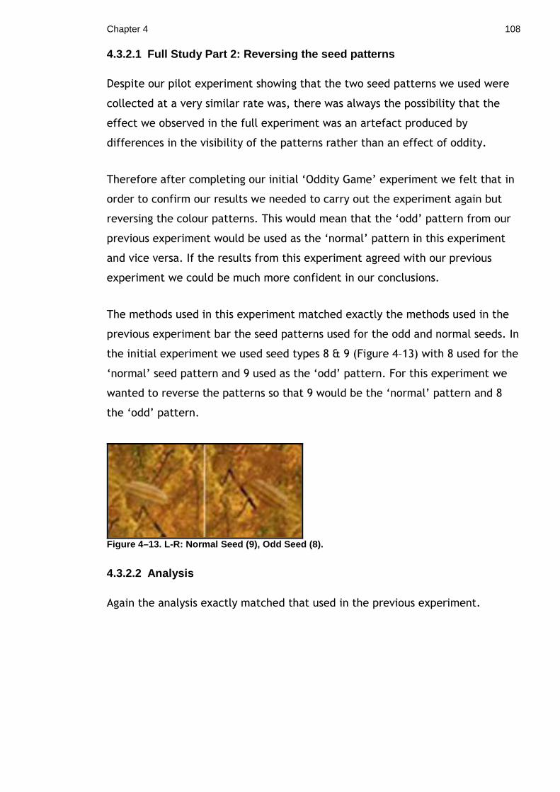
Chapter 4 108
4.3.2.1 Full Study Part 2: Reversing the seed patte rns
Despite our pilot experiment showing that the two seed patterns we used were
collected at a very similar rate was, there was always the possibility that the
effect we observed in the full experiment was an artefact produced by
differences in the visibility of the patterns rather than an effect of oddity.
Therefore after completing our initial ‘Oddity Game’ experiment we felt that in
order to confirm our results we needed to carry out the experiment again but
reversing the colour patterns. This would mean that the ‘odd’ pattern from our
previous experiment would be used as the ‘normal’ pattern in this experiment
and vice versa. If the results from this experiment agreed with our previous
experiment we could be much more confident in our conclusions.
The methods used in this experiment matched exactly the methods used in the
previous experiment bar the seed patterns used for the odd and normal seeds. In
the initial experiment we used seed types 8 & 9 (Figure 4–13) with 8 used for the
‘normal’ seed pattern and 9 used as the ‘odd’ pattern. For this experiment we
wanted to reverse the patterns so that 9 would be the ‘normal’ pattern and 8
the ‘odd’ pattern.
Figure 4–13. L-R: Normal Seed (9), Odd Seed (8).
4.3.2.2 Analysis
Again the analysis exactly matched that used in the previous experiment.
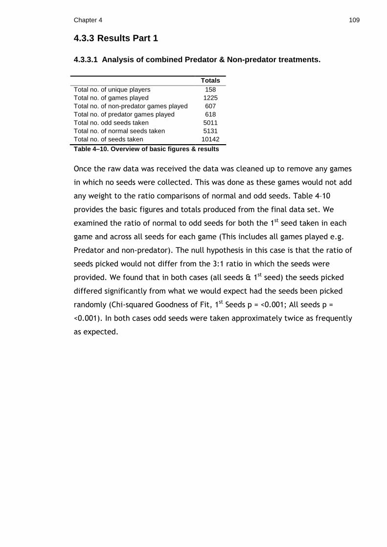
Chapter 4 109
4.3.3 Results Part 1
4.3.3.1 Analysis of combined Predator & Non-predato r treatments.
Totals Total no. of unique players 158 Total no. of games played 1225 Total no. of non-predator games played 607 Total no. of predator games played 618 Total no. odd seeds taken 5011 Total no. of normal seeds taken 5131 Total no. of seeds taken 10142
Table 4–10. Overview of basic figures & results
Once the raw data was received the data was cleaned up to remove any games
in which no seeds were collected. This was done as these games would not add
any weight to the ratio comparisons of normal and odd seeds. Table 4–10
provides the basic figures and totals produced from the final data set. We
examined the ratio of normal to odd seeds for both the 1st seed taken in each
game and across all seeds for each game (This includes all games played e.g.
Predator and non-predator). The null hypothesis in this case is that the ratio of
seeds picked would not differ from the 3:1 ratio in which the seeds were
provided. We found that in both cases (all seeds & 1st seed) the seeds picked
differed significantly from what we would expect had the seeds been picked
randomly (Chi-squared Goodness of Fit, 1st Seeds p = <0.001; All seeds p =
<0.001). In both cases odd seeds were taken approximately twice as frequently
as expected.
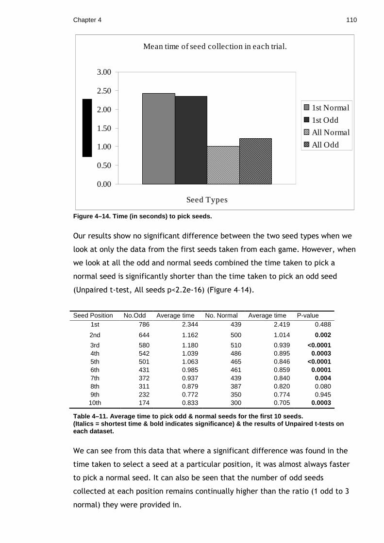
Chapter 4 110
Mean time of seed collection in each trial.
0.00
0.50
1.00
1.50
2.00
2.50
3.00
Seed Types
1st Normal
1st Odd
All Normal
All Odd
Figure 4–14. Time (in seconds) to pick seeds.
Our results show no significant difference between the two seed types when we
look at only the data from the first seeds taken from each game. However, when
we look at all the odd and normal seeds combined the time taken to pick a
normal seed is significantly shorter than the time taken to pick an odd seed
(Unpaired t-test, All seeds p<2.2e-16) (Figure 4–14).
Seed Position No.Odd Average time No. Normal Average time P-value 1st 786 2.344 439 2.419 0.488
2nd 644 1.162 500 1.014 0.002
3rd 580 1.180 510 0.939 <0.0001 4th 542 1.039 486 0.895 0.0003 5th 501 1.063 465 0.846 <0.0001 6th 431 0.985 461 0.859 0.0001 7th 372 0.937 439 0.840 0.004 8th 311 0.879 387 0.820 0.080 9th 232 0.772 350 0.774 0.945 10th 174 0.833 300 0.705 0.0003
Table 4–11. Average time to pick odd & normal seeds for the first 10 seeds. (Italics = shortest time & bold indicates significance) & t he results of Unpaired t-tests on each dataset.
We can see from this data that where a significant difference was found in the
time taken to select a seed at a particular position, it was almost always faster
to pick a normal seed. It can also be seen that the number of odd seeds
collected at each position remains continually higher than the ratio (1 odd to 3
normal) they were provided in.
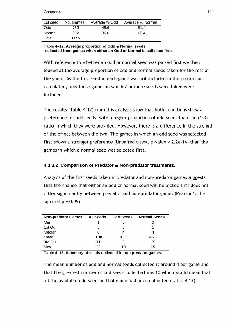
Chapter 4 111
1st seed No. Games Average % Odd Average % Normal Odd 753 48.6 51.4 Normal 392 36.6 63.4 Total 1145
Table 4–12. Average proportion of Odd & Normal seed s -collected from games when either an Odd or Normal is collected first.
With reference to whether an odd or normal seed was picked first we then
looked at the average proportion of odd and normal seeds taken for the rest of
the game. As the first seed in each game was not included in the proportion
calculated, only those games in which 2 or more seeds were taken were
included.
The results (Table 4–12) from this analysis show that both conditions show a
preference for odd seeds, with a higher proportion of odd seeds than the (1:3)
ratio in which they were provided. However, there is a difference in the strength
of the effect between the two. The games in which an odd seed was selected
first shows a stronger preference (Unpaired t-test, p-value < 2.2e-16) than the
games in which a normal seed was selected first.
4.3.3.2 Comparison of Predator & Non-predator treat ments.
Analysis of the first seeds taken in predator and non-predator games suggests
that the chance that either an odd or normal seed will be picked first does not
differ significantly between predator and non-predator games (Pearson’s chi-
squared p = 0.95).
Non-predator Games All Seeds Odd Seeds Normal Seeds Min 1 0 0 1st Qu. 5 3 1 Median 8 4 4 Mean 8.38 4.11 4.28 3rd Qu. 11 6 7 Max 22 10 15
Table 4–13. Summary of seeds collected in non-preda tor games.
The mean number of odd and normal seeds collected is around 4 per game and
that the greatest number of odd seeds collected was 10 which would mean that
all the available odd seeds in that game had been collected (Table 4–13).
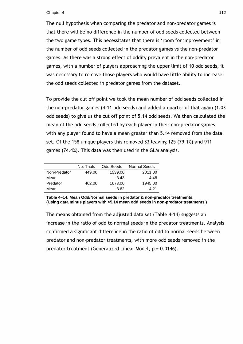
Chapter 4 112
The null hypothesis when comparing the predator and non-predator games is
that there will be no difference in the number of odd seeds collected between
the two game types. This necessitates that there is ‘room for improvement’ in
the number of odd seeds collected in the predator games vs the non-predator
games. As there was a strong effect of oddity prevalent in the non-predator
games, with a number of players approaching the upper limit of 10 odd seeds, it
was necessary to remove those players who would have little ability to increase
the odd seeds collected in predator games from the dataset.
To provide the cut off point we took the mean number of odd seeds collected in
the non-predator games (4.11 odd seeds) and added a quarter of that again (1.03
odd seeds) to give us the cut off point of 5.14 odd seeds. We then calculated the
mean of the odd seeds collected by each player in their non-predator games,
with any player found to have a mean greater than 5.14 removed from the data
set. Of the 158 unique players this removed 33 leaving 125 (79.1%) and 911
games (74.4%). This data was then used in the GLM analysis.
No. Trials Odd Seeds Normal Seeds Non-Predator 449.00 1539.00 2011.00 Mean 3.43 4.48 Predator 462.00 1673.00 1945.00 Mean 3.62 4.21
Table 4–14. Mean Odd/Normal seeds in predator & non -predator treatments. (Using data minus players with >5.14 mean odd seeds in non-predator treatments.)
The means obtained from the adjusted data set (Table 4–14) suggests an
increase in the ratio of odd to normal seeds in the predator treatments. Analysis
confirmed a significant difference in the ratio of odd to normal seeds between
predator and non-predator treatments, with more odd seeds removed in the
predator treatment (Generalized Linear Model, p = 0.0146).
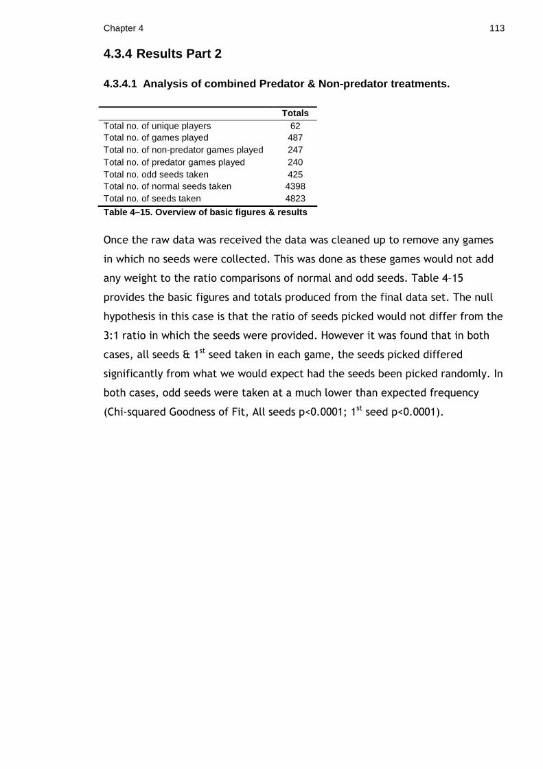
Chapter 4 113
4.3.4 Results Part 2
4.3.4.1 Analysis of combined Predator & Non-predato r treatments.
Totals Total no. of unique players 62 Total no. of games played 487 Total no. of non-predator games played 247 Total no. of predator games played 240 Total no. odd seeds taken 425 Total no. of normal seeds taken 4398 Total no. of seeds taken 4823
Table 4–15. Overview of basic figures & results
Once the raw data was received the data was cleaned up to remove any games
in which no seeds were collected. This was done as these games would not add
any weight to the ratio comparisons of normal and odd seeds. Table 4–15
provides the basic figures and totals produced from the final data set. The null
hypothesis in this case is that the ratio of seeds picked would not differ from the
3:1 ratio in which the seeds were provided. However it was found that in both
cases, all seeds & 1st seed taken in each game, the seeds picked differed
significantly from what we would expect had the seeds been picked randomly. In
both cases, odd seeds were taken at a much lower than expected frequency
(Chi-squared Goodness of Fit, All seeds p<0.0001; 1st seed p<0.0001).
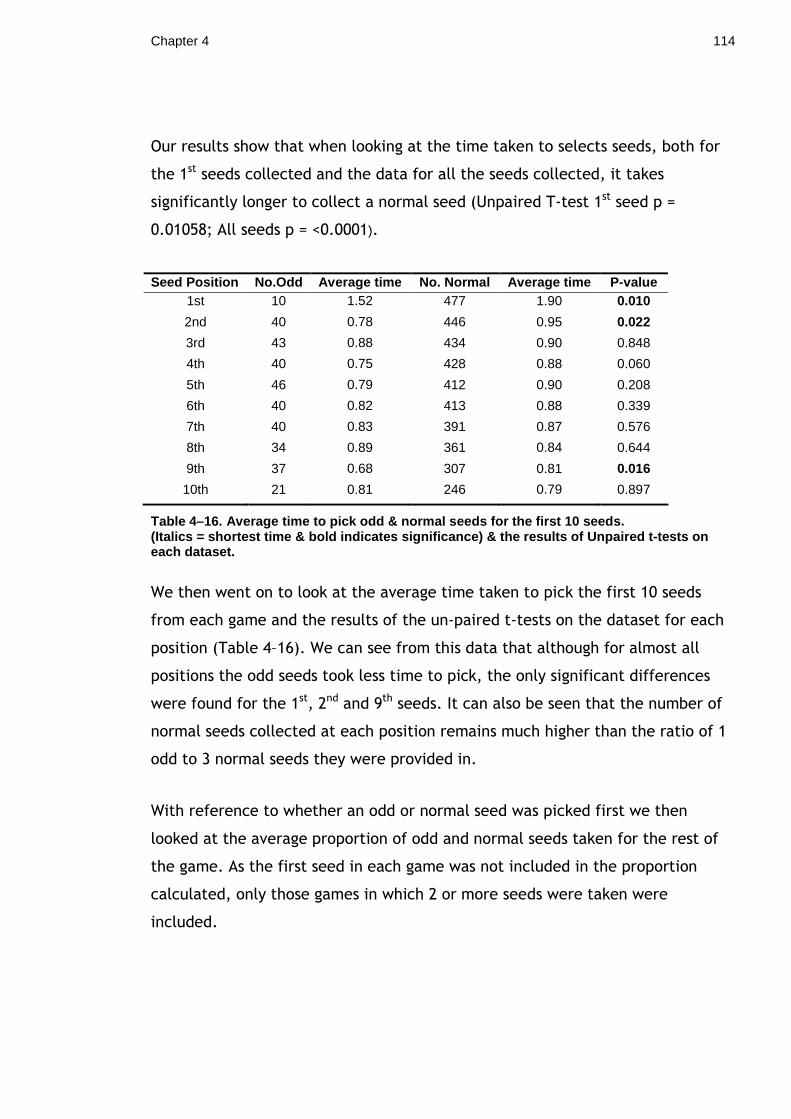
Chapter 4 114
Our results show that when looking at the time taken to selects seeds, both for
the 1st seeds collected and the data for all the seeds collected, it takes
significantly longer to collect a normal seed (Unpaired T-test 1st seed p =
0.01058; All seeds p = <0.0001).
Seed Position No.Odd Average time No. Normal Average time P-value 1st 10 1.52 477 1.90 0.010
2nd 40 0.78 446 0.95 0.022
3rd 43 0.88 434 0.90 0.848
4th 40 0.75 428 0.88 0.060
5th 46 0.79 412 0.90 0.208
6th 40 0.82 413 0.88 0.339
7th 40 0.83 391 0.87 0.576
8th 34 0.89 361 0.84 0.644
9th 37 0.68 307 0.81 0.016
10th 21 0.81 246 0.79 0.897
Table 4–16. Average time to pick odd & normal seeds for the first 10 seeds. (Italics = shortest time & bold indicates significance) & t he results of Unpaired t-tests on each dataset.
We then went on to look at the average time taken to pick the first 10 seeds
from each game and the results of the un-paired t-tests on the dataset for each
position (Table 4–16). We can see from this data that although for almost all
positions the odd seeds took less time to pick, the only significant differences
were found for the 1st, 2nd and 9th seeds. It can also be seen that the number of
normal seeds collected at each position remains much higher than the ratio of 1
odd to 3 normal seeds they were provided in.
With reference to whether an odd or normal seed was picked first we then
looked at the average proportion of odd and normal seeds taken for the rest of
the game. As the first seed in each game was not included in the proportion
calculated, only those games in which 2 or more seeds were taken were
included.
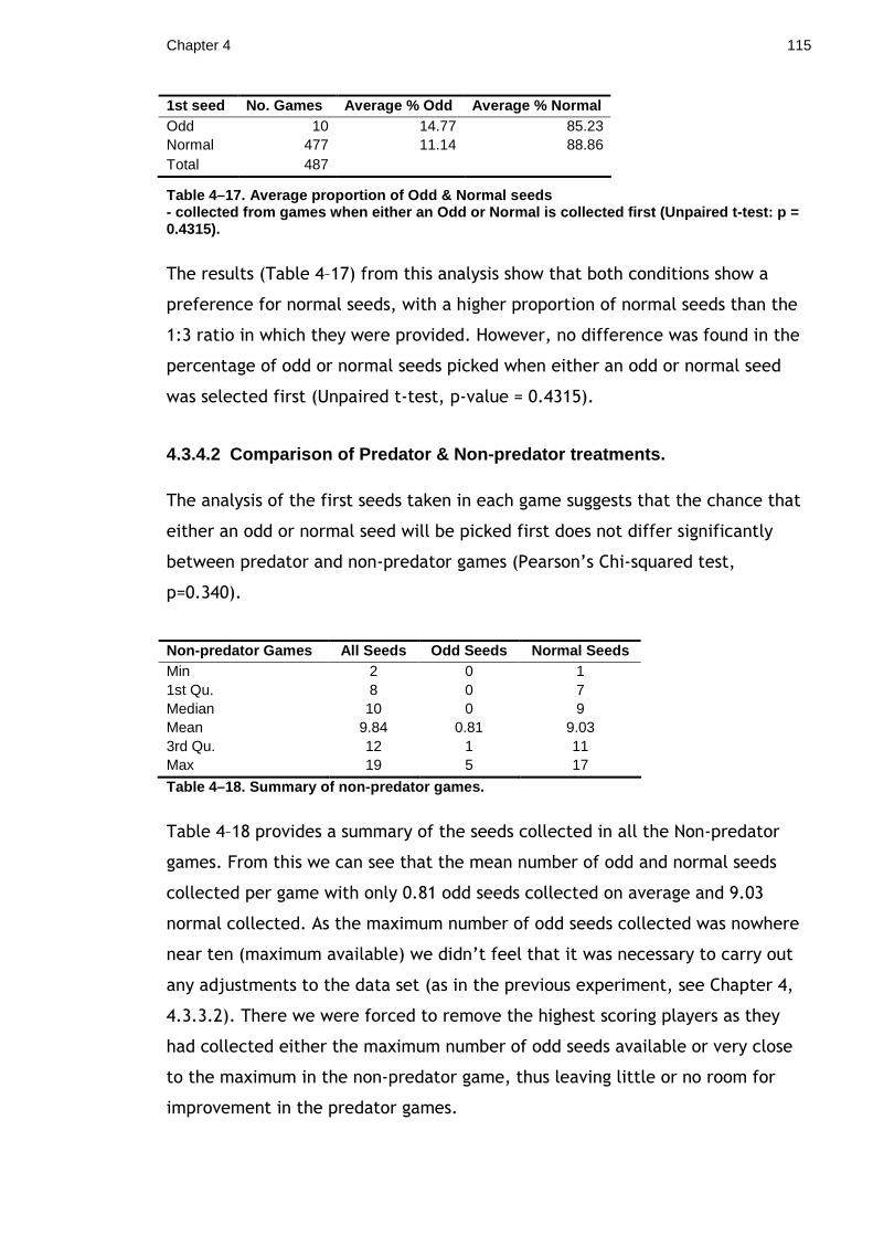
Chapter 4 115
1st seed No. Games Average % Odd Average % Normal Odd 10 14.77 85.23 Normal 477 11.14 88.86 Total 487
Table 4–17. Average proportion of Odd & Normal seed s - collected from games when either an Odd or Normal is collected first (Unpaired t-test: p = 0.4315).
The results (Table 4–17) from this analysis show that both conditions show a
preference for normal seeds, with a higher proportion of normal seeds than the
1:3 ratio in which they were provided. However, no difference was found in the
percentage of odd or normal seeds picked when either an odd or normal seed
was selected first (Unpaired t-test, p-value = 0.4315).
4.3.4.2 Comparison of Predator & Non-predator treat ments.
The analysis of the first seeds taken in each game suggests that the chance that
either an odd or normal seed will be picked first does not differ significantly
between predator and non-predator games (Pearson’s Chi-squared test,
p=0.340).
Non-predator Games All Seeds Odd Seeds Normal Seeds Min 2 0 1 1st Qu. 8 0 7 Median 10 0 9 Mean 9.84 0.81 9.03 3rd Qu. 12 1 11 Max 19 5 17
Table 4–18. Summary of non-predator games.
Table 4–18 provides a summary of the seeds collected in all the Non-predator
games. From this we can see that the mean number of odd and normal seeds
collected per game with only 0.81 odd seeds collected on average and 9.03
normal collected. As the maximum number of odd seeds collected was nowhere
near ten (maximum available) we didn’t feel that it was necessary to carry out
any adjustments to the data set (as in the previous experiment, see Chapter 4,
4.3.3.2). There we were forced to remove the highest scoring players as they
had collected either the maximum number of odd seeds available or very close
to the maximum in the non-predator game, thus leaving little or no room for
improvement in the predator games.
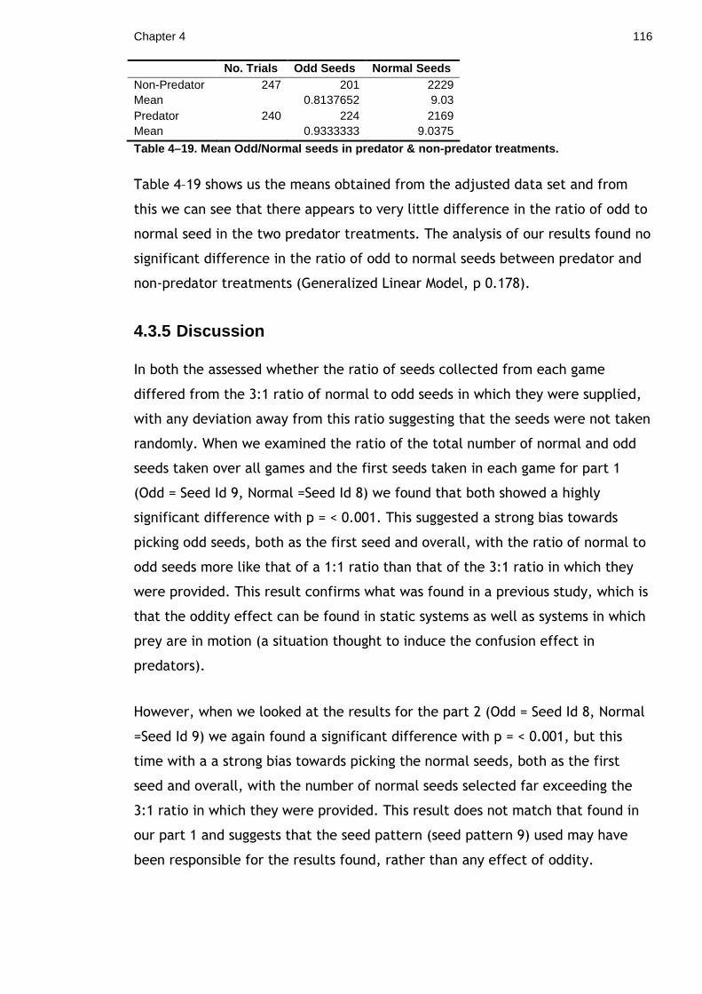
Chapter 4 116
No. Trials Odd Seeds Normal Seeds Non-Predator 247 201 2229 Mean 0.8137652 9.03 Predator 240 224 2169 Mean 0.9333333 9.0375
Table 4–19. Mean Odd/Normal seeds in predator & non -predator treatments.
Table 4–19 shows us the means obtained from the adjusted data set and from
this we can see that there appears to very little difference in the ratio of odd to
normal seed in the two predator treatments. The analysis of our results found no
significant difference in the ratio of odd to normal seeds between predator and
non-predator treatments (Generalized Linear Model, p 0.178).
4.3.5 Discussion
In both the assessed whether the ratio of seeds collected from each game
differed from the 3:1 ratio of normal to odd seeds in which they were supplied,
with any deviation away from this ratio suggesting that the seeds were not taken
randomly. When we examined the ratio of the total number of normal and odd
seeds taken over all games and the first seeds taken in each game for part 1
(Odd = Seed Id 9, Normal =Seed Id 8) we found that both showed a highly
significant difference with p = < 0.001. This suggested a strong bias towards
picking odd seeds, both as the first seed and overall, with the ratio of normal to
odd seeds more like that of a 1:1 ratio than that of the 3:1 ratio in which they
were provided. This result confirms what was found in a previous study, which is
that the oddity effect can be found in static systems as well as systems in which
prey are in motion (a situation thought to induce the confusion effect in
predators).
However, when we looked at the results for the part 2 (Odd = Seed Id 8, Normal
=Seed Id 9) we again found a significant difference with p = < 0.001, but this
time with a a strong bias towards picking the normal seeds, both as the first
seed and overall, with the number of normal seeds selected far exceeding the
3:1 ratio in which they were provided. This result does not match that found in
our part 1 and suggests that the seed pattern (seed pattern 9) used may have
been responsible for the results found, rather than any effect of oddity.
Chapter 4 117
We then examined the time it taken for a seed to be picked. For the first seed in
each game this was taken to be the time from the start of the game until the
first seed was picked and for all other seeds it was the time from the last seed
taken until the seed was picked. We hypothesised that predators use the oddity
effect to decrease the time taken to isolate and pick prey from a group,
therefore for this to be true we would expect odd seeds to be picked faster than
normal seeds. Looking at Part 1 first of all we found no significant difference
was between odd and normal seeds the time taken for the first seed to be
selected in each game (Figure 4–14). This suggested that despite there being
considerably fewer odd seeds within the group, it does not take any longer for
them to be selected. When we then analysed the results from all the seeds taken
over all games the relationship changed with odd seeds now taking significantly
longer to select than a normal seed (p = < 2.2E-16), with the mean odd time 0.25
seconds slower than the normal seeds. This might suggest a unique choice
heuristic with odd seeds chosen preferentially it does not increase the time to
select until the pool of odd prey begins to be depleted.
We then looked at the results for part 2 where the seed designs had been
reversed for odd and normal the results seem to support our hypothesis that
preferentially selecting odd seeds maybe an adaptation to speed up prey
acquisition. For the first seed taken from each game it was found that there was
a significant (p = 0.01) difference between odd and normal seeds, with the mean
odd time found to be 0.38 seconds faster than normal seeds. We then analysed
the time results for all seeds taken over all the games played & we found that
once again there is a significant difference with the mean odd time 0.17 seconds
faster than the mean normal time.
To look more closely at this we then compared the time taken to pick seeds at
each position for the first 10 seeds in each game using Un-paired t-tests and
comparing the average time. This showed that again there are significant
differences between the odd and normal seed, but that almost all positions it
would be quicker to pick a normal seed. However, despite the apparent
disadvantage of taking longer to select, odd seeds continued to be selected
preferentially in higher numbers than we would expect by chance alone. We
again checked this against the results from the reversed pattern results and
again we found a significant difference between the selection times (1st, 2nd &
Chapter 4 118
9th seeds), with odd seeds taking less time to select than normal seeds (Table 4–
11) . That it is still quicker to select the odd seeds in part 2 despite normal
seeds being more numerous and more conspicuous adds weight to the hypothesis
that a preference for oddity may reduce selection deliberation time.
Next we examined whether having an odd or normal seed being selected first
had any relation to the total proportion of odd or normal seeds taken in each
game. We hypothesised that those players that selected an odd seed first may
continue to show an increased preference for oddity in their seed selection. Our
results suggest that the first seed selected in each game does appear to have an
effect or relationship with the seeds that are subsequently selected (Table 4–
12). While both conditions show a higher than expected number of odd seeds
picked, the effect appears to be stronger in those games where an odd seed is
selected first. However, when we looked at the results for part 2 we that the
first seed selected did not have any effect or relationship with the seeds that
are subsequently selected (Table 4–17). Due to the confounding effect of the
difference in conspicuousness between the seed patterns used we can not say
whether there is any effect.
The second part of our experiment was to look at whether there was any
difference between the predator and non-predator games. The purpose of this
was to examine whether the oddity effect would be stronger in situations where
attention is divided between prey selection and scanning for predators. Analysis
of the first seeds taken from each game for both parts 1 and 2 showed no
significant difference between the ratios of odd to normal seeds taken from the
two sets of games. This result does not support our hypothesis, although due to
what appears to be a very strong effect of seed pattern it might be that any
other effect are effectively drowned out.
To examine this further we wanted to look at the ratio of all the seeds taken in
each game. However, when looking at the summary statistics for part 1, the
non-predator games (Table 4–13) it was realised that there were a number of
individuals that removed a very high proportion of the odd seeds available in the
control (non-predator) games and in some cases 100%. Obviously this would
mean that for those players there is little or no room to increase the number of
odd seeds they collect in the predator games. Since including these players in
Chapter 4 119
the analysis could mask an increase shown by the rest of the players it was
decided that they should be removed from this analysis (see methods for
details). This was found to not be necessary for the part 2 results.
A model was then used to compare the ratios of odd to normal seeds across the
two game types. For part 1 the analysis showed that there was a significant
increase in the ratio of odd seeds taken in the predator games (Table 4–14).
However, for part 2 where the seed patterns had been swapped round there was
no significant change in the ratio of odd seeds taken in the predator games
(Table 4–19). This suggests that the difference we found in part 1 is likely to be
caused by a difference in the level of conspicuousness between the seed
patterns and does not provide support for the hypothesis that a preference for
odd prey may be a way to reduce selection time when attention must be split
between prey selection and scanning for predators.
Previous studies that have examined the behaviour of foraging birds have
suggested that they are limited by the amount of attention they can give to both
foraging and scanning for predators and that this limit in attention may be a
major cause of mortality in the wild (Dukas and Kamil, 2000). This may provide
us with some insight as to why the oddity effect would still be evident in prey
selection by predators from grouped but static prey, where we would expect
them to suffer less from the confusion effect. This combined with knowledge
that the preference for odd seeds continues even when apparently
disadvantageous suggest that what we may be seeing is the effects of Waite’s
(2008) suggested ‘odd choice heuristic’. This rule of thumb should dictate that
oddity should always be selected preferentially, potentially short-cutting the
deliberating phase of prey selection. This would allow a greater proportion of
the limited attention a predator has to be put towards scanning for danger and
thereby increasing survival.
The use of search images may also have a role to play here, with predators that
using shape, colour and pattern to form search images to increase foraging
efficiency (Pietrewicz and Kamil, 1979). Another paper by Dukas and Kamil
(2001) examined the effect of dividing attention by searching for two distinct
cryptic prey types. For this they used blue jays (Cyanocitta cristata) trained to
search for two types of cryptic prey on a computer monitor. In the first

Chapter 4 120
treatment cues were given to signal which prey item to search for and no cost
was seen in switching between searching for each prey type. Conversely, in the
second treatment where no cues where given and the jays had to divide their
attention between searching for two prey types they paid for this with a lower
detection rate. This might suggest that once a predator has locked in to using
the odd search image there would be penalties for switching to a new search
image.
In summary our results suggest that selecting odd individuals takes less time
than selecting normal group members and supports the hypothesis that selecting
odd prey may be an adaptation to reduce selection time. While in this case we
use the term seeds when describing the on screen stimuli these results are
equally applicable to lepidopteran larvae and other prey species that rely on
crypsis. Unfortunately, due to the differences in conspicuousness we can not say
anything further. If as we suspect the pattern used for the normal seed in this
case was more conspicuous this may lend even more weight to the idea that a
preference for oddity reduces selection deliberation time i.e. that despite
normal seeds being more numerous and being more visible it is quick to pick an
odd seed.
In future we need to find a better way to assess the conspicuousness of the
seeds patterns we use. The results from both experiments along with the pilot
test we carried out suggest that the context in which the seed patterns are
viewed can strongly affect the predation rate. In this case we found that while
the seeds patterns have very similar predation rates when presented in single
pattern groups, when we then presented them as part of a mixed group the
differences in conspicuousness became far more explicit. Therefore we propose
testing the seed patterns in pairs with a 50:50 pattern mix. This should allow us
to select 2 patterns which appear equally conspicuous when presented together.
Our findings on the effect of group context on the conspicuousness of cryptic
patterning, also has implications for crypsis in the field. It potentially points to a
scenario in which two groups combine and despite both having previously
suffered similar levels of predation, one phenotype may find that it now suffers
a far higher percentage of the predation burden.
Chapter 5 121
Chapter 5. Protection by association: Evidence for Aposematic commensalism
Many foragers hunt by sight, using shape, colour and pattern to form search
images which increase foraging efficiency (Pietrewicz and Kamil, 1979). Most
avian foragers are well equipped with sensitive tetrachromatic colour vision to
search out and target prey (Finger and Burkhardt, 1994).
There are a number of ways that colouration and pattern are utilised by
organisms to reduce predation and they generally fall in to three categories; (1)
Crypsis, in which the prey reduces predation by avoiding detection by predators
entirely; (2) aposematism, where the prey is easily detected but advertise their
unsuitability as prey (Ruxton et al., 2004); and (3) masquerade, in which the
prey may be detected but is misclassified as something non-edible (Skelhorn et
al., 2010b). In the first category we include any type of crypsis or camouflage,
such as background matching and/or disruptive patterning. The effect of these
patterns is to hinder detection of an organism so that predators pass by without
detecting their presence. In the case of disruptive patterning, this is achieved by
breaking up an organisms distinctive outline (Stevens and Merilaita, 2009). The
next two categories do not prevent detection of the organism, but change a
predator’s estimation of profitability so that they choose not to attack. This is
achieved either by ‘masquerade’ where colouration or patterning mimic the
appearance of something inedible such as a twig or bird faeces (Skelhorn et al.,
2010b) or with the use of aposematic signals such as conspicuous behaviour,
odour, sound or colouration to indicate unprofitability and advertise
defences(Cott, 1940; Poulton, 1890). The conspicuousness nature of aposematic
displays is thought to (1) enable predators to easily distinguish defended prey
from undefended prey and (2) impose costs that only prey displaying an ‘honest’
signal of unsuitability can afford, such as increased detection rates(Sherratt and
Beatty, 2003).
Effective aposematic signalling provides great advantages for survival and
therefore, great opportunities for cheats. Why go to the expense of developing
secondary defences when, by mimicking the characteristic warning signals of an
Chapter 5 122
unpalatable or otherwise defended model organism, you can benefit without
them? This type of mimicry is called Batesian mimicry. Nonetheless, it is not
necessary for mimics to perfectly match all aspects of the model’s patterning
because even imperfect mimicry provides some protection(Kikuchi and Pfennig).
However, dishonest signals, like those of Batesian mimics, can change the
effectiveness of the warning signal. A number of studies have shown that, as the
ratio of mimics to models increases, it reduces the effectiveness of the warning
signal and predation rates for both groups increase(Ruxton et al., 2004).
To understand selection for the evolution of Batesian mimicry we must evaluate
the fitness consequences of being non-mimetic. How does being in close
proximity to aposematic prey affect undefended cryptic prey? One may predict
that they would suffer greater predation, with the aposematic prey drawing the
attention of predators to the location, which then turn to the more palatable
and profitable prey once identified. Alternatively, non-signalling and palatable
prey may benefit from their proximity to their aposematic neighbours. A
laboratory study conducted by Mappes, Tuomi & Alatalo (1999) investigated this
issue using wild caught birds presented with aposematic (unpalatable) and
palatable prey in groups of either purely palatable, aposematic or mixed prey
types. Their results suggest that palatable prey, in fact, benefit from a
reduction in predation risk when grouped with aposematic prey through
‘aposematic commensalism’. That is, palatable prey appear to benefit from
being offered alongside unpalatable prey even when there was no strong
similarity in appearance between the prey types. This might occur if predators
avoid locations where they have had noxious experiences, or if an aversive
experience causes a period of disinterest in food of any kind. Importantly,
commensal relationships and associations between cryptic and aposematic
species may be an important ‘first step’ towards the evolution of Batesian
mimicry.
A parallel to this type of relationship, where one species benefits from
association with another, may be found in botany. In this case, ‘magnet species’
(Molina-Montenegro et al., 2008) that are particularly attractive to pollinators
do not divert most of the pollinators away from less attractive plants nearby, as
may be expected. In fact, they appear in some cases to increase the number of
visits those plants receive. This means that less attractive species can increase

Chapter 5 123
their chances of being pollinated and, therefore, increase the number of seeds
they produce, just by growing in close proximity to more attractive species.
Mappes’ original research (Mappes et al., 1999) was conducted in a lab setting
and under idealised conditions with prey items presented either singly or in pairs
on a wooden plate. We, therefore, decided that it would be beneficial to
generalise this study with a larger sample size and with the prey items presented
in a more ecologically realistic setting to examine whether the observed effect
would still be found in a less carefully controlled environment. Additionally, in
the original experiment all 5 treatments, namely, (1) 1 aposematic prey item;
(2) 1 palatable prey item; (3) 2 aposematic prey items; (4) 2 palatable prey
items; (5) 1 palatable and 1 aposematic prey items were presented
simultaneously, whereas, in nature predator-prey encounters are more likely to
occur sequentially. The change from simultaneous to sequential presentation
changes the predators’ task from that of a comparison followed by a decision on
whether to attack, to purely a choice between attacking or leaving without
feeding. In a lab experiment like this, birds may also learn that whichever item
they do not choose is removed, making the comparison stage a more important
step in the process. We might also want to consider that predators may use the
number of prey presented as a cue to the general availability of food, with a
choice between two or more prey items indicating a greater availability of food.
This may mean that when presented with an individual food item there is a
greater perceived uncertainty in the future availability of food and therefore
greater pressure to attack.
We further tested the hypothesis that non-conspicuous and undefended prey
could reduce their predation rate by associating with aposematic prey by using
groups of sunflower seeds (5 or 10 seeds) made either, conspicuous and
unpalatable (UnP), or cryptic and palatable (P). The seeds were presented in
mixed or single treatment groups within a field setting and the local wild bird
assemblage was allowed to select and remove seeds, at will, over a set period of
time. This allowed us to compare the survival rate of each seed/group type at
the end of each trial.

Chapter 5 124
5.1.1 Methods & Materials
This experiment was conducted between October 2010 and March 2011 in areas
of park land in the centre of Glasgow, Scotland (Latitude: 55° 52' N, Longitude:
4° 15' W).
Groups of coloured seeds were left out at selected sites at 9am and their
remaining numbers were checked at 4pm. There were 20 replicates of each of
the 5 different treatments used (Table 5–1). This included 4 groups of
homogenous colouring (i.e. all seeds within each group being of the same
colouring & palatability) and 1 treatment of mixed seeds, the groups of which
were composed of half and half of each colour being used.
Treatment Unpalatable Palatable Total 1 5 5 10 2 5 0 5 3 0 5 5 4 10 0 10 5 0 10 10
Table 5–1. Number and type of seed in each treatmen t Group.
To ensure that the seeds from each group were spread evenly over the desired
area, a circular cardboard ‘stencil’ was cut to 10 cm in diameter and used to
ensure the grouped seeds remained within the set area. The pre-prepared seed
groups were then sprinkled from a height of at least 10cm to ensure an even but
random distribution. Treatments were placed out in a random order with a
minimum of 10 metres between each group. To aid in collection of groups
following experiments, a coloured golf tee was placed three paces to the north
of each group. As an extra precaution, a brief note of the golf tee’s location was
also taken.
The sites were revisited at 4pm each day and the remaining seeds were counted
and recorded. To ensure that missing seeds could be considered to be eaten and
not just displaced; searching continued for 5 minutes after the last seed had
been found. Seeds recovered were also examined to see if they had been
‘discreetly’ eaten (where the kernel had been removed via a small hole in the
husk which on casual inspection may look intact).
Chapter 5 125
There were three parts to this experiment. In part one we used unpalatable red
seeds and palatable green seeds. This was carried out over 1 month from 28th
October 2010 at Site 1 with one replicate of each treatment set out per day (a
total of 5 groups of seeds per day over 20 days). In part 2, using the same
methodology, we carried out the reciprocal experiment from 15th January 2011
to 6th February at Site 2, with unpalatable green seeds and palatable red seeds.
As we expected the incongruity of the colour and palatability to reduce the
effect of the conspicuous colouring and unpalatability on the predation rate we
carried out an extra 10 replicates (30 in total). We carried out the final part
from 7th February to 1st March, at site 1, with 20 replicates using palatable green
and red seeds. In all cases, it was assumed that the green seeds were cryptic
against the green background and that the red seeds were more conspicuous.
However, our design was counterbalanced for colour and, thus, our
interpretation was not contingent on the validity of these assumptions.
5.1.1.1 Site selection
The sites were selected for a combination of high bird activity and reduced
human activity levels (human activity could not be avoided all together due to
the inner city location). In particular, areas known to have regular bird feeding
activity by humans were avoided, as these were likely to have many human
visitors. While the treatment groups were not watched throughout the day a
number of different bird species were observed close to or in the immediate
area including blackbirds (Turdus merula), bluetits (Cyanistes caeruleus),
bullfinch (Pyrrhula pyrrhula), carrion crow (Corvus corone), house sparrows
(Passer domesticus), magpie (Pica pica), robin (Erithacus rubecula), rock pigeon
(Columba livia), starling (Sturnus vulgaris) and wood pigeon (Columba
palumbus). From observations carried out in previous unpublished work we knew
that these species have also been seen to take interest in and feed from seed
groups left out and that consumption of experimental seeds by mammals, such
as grey squirrels (Sciurus carolinensis), is extremely rare.
The two sites selected, Site 1 (55°52'24.92"N 4°16'49.50"W) and Site 2
(55°52'54.47"N 4°17'27.62"W), were within 1 mile of each other. Both sites
were of a sufficiently large area to prevent the need for repeated trials in the
same space and overlap of area usage was minimised. In the weeks prior to the
Chapter 5 126
experiment, wild bird seed was scattered to encourage birds to return to the
sites throughout the winter months. Following the first experiment, a new site
was chosen in which to conduct the second experiment in an attempt to ensure
that different birds would be exposed to the new treatments and, thus, the
problems with learning and conditioning would be greatly reduced. To maximise
undisturbed foraging time seed groups were placed on open areas of grass, away
from footpaths and other areas of high traffic. Trials were not conducted during
periods of heavy rainfall where muddy conditions would make differentiating
seed colour difficult and would reduce feeding activity in the bird population.
Treatments were also not conducted during the extended snowfall in late
November and December 2010.
5.1.1.2 Seed Treatments
Four types of bait were prepared, 1) palatable green seeds; 2) palatable red
seeds; 3) unpalatable green seeds; and 4) unpalatable red seeds. In addition to
their colouring, the ‘unpalatable’ seeds were treated with quinine
hydrochloride, a chemical substance with a pronounced bitter taste known to be
aversive to both domestic and wild birds (Halpin et al., 2008; Rowland et al.,
2010; Skelhorn et al., 2008; Speed et al., 2000).
Standard striped sunflower seeds were dyed using Sugar Flairs food dye Holly
Green and Red Extra. The dye concentrates were diluted using 200ml water with
75ml dye gel. 165g of striped sunflower seeds were mixed with 20ml of the dye
solution and 200ml of water. This was brought to a simmer and left for 15mins,
stirring occasionally. To make the unpalatable seeds 2 tablespoons (~34g) of
quinine were added to the water and dye before simmering. The liquid was
reduced as much as possible and, after simmering, the seeds and any remaining
liquid were spread out on a baking tray to ensure that little dye or quinine was
lost. To dry the seeds out completely a domestic oven was set to its lowest
setting (50°C) and the seeds were spread on a baking tray. The seeds were
checked and turned regularly. Once all traces of surface water had evaporated
and the seeds were dry they were removed from the oven. The seeds retained
their striped pattern after this treatment.
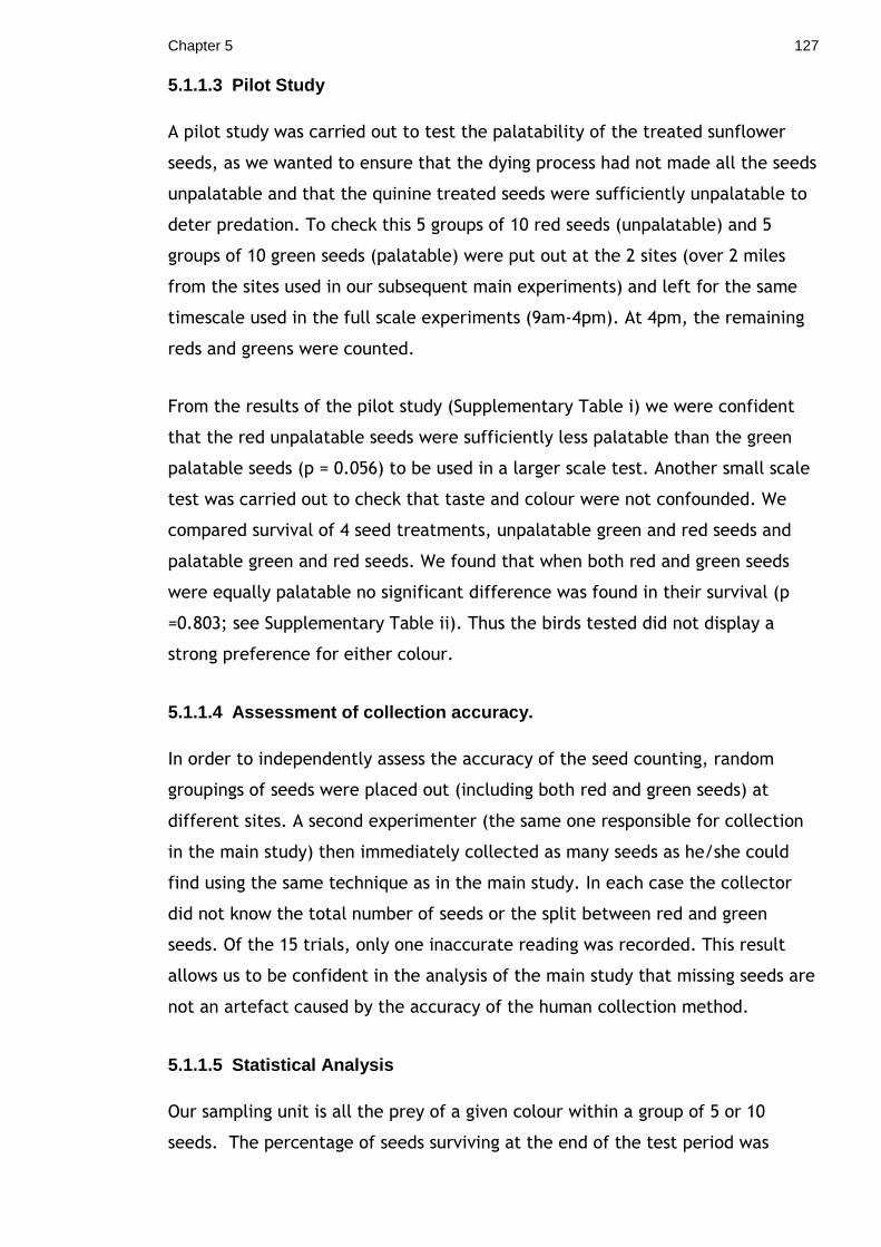
Chapter 5 127
5.1.1.3 Pilot Study
A pilot study was carried out to test the palatability of the treated sunflower
seeds, as we wanted to ensure that the dying process had not made all the seeds
unpalatable and that the quinine treated seeds were sufficiently unpalatable to
deter predation. To check this 5 groups of 10 red seeds (unpalatable) and 5
groups of 10 green seeds (palatable) were put out at the 2 sites (over 2 miles
from the sites used in our subsequent main experiments) and left for the same
timescale used in the full scale experiments (9am-4pm). At 4pm, the remaining
reds and greens were counted.
From the results of the pilot study (Supplementary Table i) we were confident
that the red unpalatable seeds were sufficiently less palatable than the green
palatable seeds (p = 0.056) to be used in a larger scale test. Another small scale
test was carried out to check that taste and colour were not confounded. We
compared survival of 4 seed treatments, unpalatable green and red seeds and
palatable green and red seeds. We found that when both red and green seeds
were equally palatable no significant difference was found in their survival (p
=0.803; see Supplementary Table ii). Thus the birds tested did not display a
strong preference for either colour.
5.1.1.4 Assessment of collection accuracy.
In order to independently assess the accuracy of the seed counting, random
groupings of seeds were placed out (including both red and green seeds) at
different sites. A second experimenter (the same one responsible for collection
in the main study) then immediately collected as many seeds as he/she could
find using the same technique as in the main study. In each case the collector
did not know the total number of seeds or the split between red and green
seeds. Of the 15 trials, only one inaccurate reading was recorded. This result
allows us to be confident in the analysis of the main study that missing seeds are
not an artefact caused by the accuracy of the human collection method.
5.1.1.5 Statistical Analysis
Our sampling unit is all the prey of a given colour within a group of 5 or 10
seeds. The percentage of seeds surviving at the end of the test period was
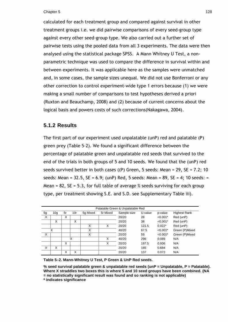
Chapter 5 128
calculated for each treatment group and compared against survival in other
treatment groups i.e. we did pairwise comparisons of every seed-group type
against every other seed-group type. We also carried out a further set of
pairwise tests using the pooled data from all 3 experiments. The data were then
analysed using the statistical package SPSS. A Mann Whitney U Test, a non-
parametric technique was used to compare the difference in survival within and
between experiments. It was applicable here as the samples were unmatched
and, in some cases, the sample sizes unequal. We did not use Bonferroni or any
other correction to control experiment-wide type 1 errors because (1) we were
making a small number of comparisons to test hypotheses derived a priori
(Ruxton and Beauchamp, 2008) and (2) because of current concerns about the
logical basis and powers costs of such corrections(Nakagawa, 2004).
5.1.2 Results
The first part of our experiment used unpalatable (unP) red and palatable (P)
green prey (Table 5–2). We found a significant difference between the
percentage of palatable green and unpalatable red seeds that survived to the
end of the trials in both groups of 5 and 10 seeds. We found that the (unP) red
seeds survived better in both cases ((P) Green, 5 seeds: Mean = 29, SE = 7.2; 10
seeds: Mean = 32.5, SE = 6.9; (unP) Red, 5 seeds: Mean = 89, SE = 4; 10 seeds: =
Mean = 82, SE = 5.3, for full table of average % seeds surviving for each group
type, per treatment showing S.E. and S.D. see Supplementary Table iii).
Palatable Green & Unpalatable Red 5g 10g 5r 10r 5g Mixed 5r Mixed Sample size U-value p-value Highest Rank X X 20/20 28 <0.001* Red (unP) X X 20/20 38 <0.001* Red (unP) X X 20/20 121.5 0.022* Red (unP)
X X 40/20 67.5 <0.001* Green (P)Mixed X X 20/20 59 <0.001* Green (P)Mixed X X 40/20 296 0.089 N/A
X X 20/20 197.5 0.936 N/A X X 20/20 185 0.684 N/A X X 20/20 137 0.072 N/A
Table 5–2. Mann-Whitney U Test, P Green & UnP Red s eeds.
% seed survival palatable green & unpalatable red s eeds (unP = Unpalatable, P = Palatable). Where X straddles two boxes this is where 5 and 10 seed groups have been combined. (NA = no statistically significant result was found and so ranking is not applicable) * indicates significance
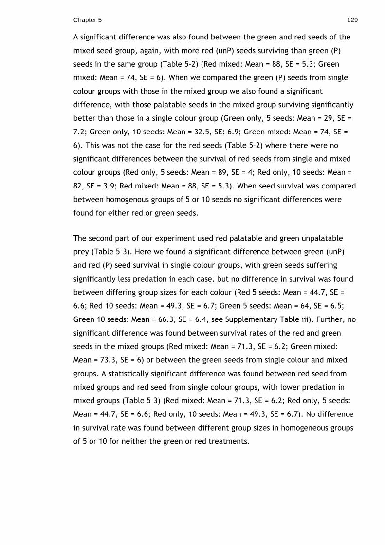
Chapter 5 129
A significant difference was also found between the green and red seeds of the
mixed seed group, again, with more red (unP) seeds surviving than green (P)
seeds in the same group (Table 5–2) (Red mixed: Mean = 88, SE = 5.3; Green
mixed: Mean = 74, SE = 6). When we compared the green (P) seeds from single
colour groups with those in the mixed group we also found a significant
difference, with those palatable seeds in the mixed group surviving significantly
better than those in a single colour group (Green only, 5 seeds: Mean = 29, SE =
7.2; Green only, 10 seeds: Mean = 32.5, SE: 6.9; Green mixed: Mean = 74, SE =
6). This was not the case for the red seeds (Table 5–2) where there were no
significant differences between the survival of red seeds from single and mixed
colour groups (Red only, 5 seeds: Mean = 89, SE = 4; Red only, 10 seeds: Mean =
82, SE = 3.9; Red mixed: Mean = 88, SE = 5.3). When seed survival was compared
between homogenous groups of 5 or 10 seeds no significant differences were
found for either red or green seeds.
The second part of our experiment used red palatable and green unpalatable
prey (Table 5–3). Here we found a significant difference between green (unP)
and red (P) seed survival in single colour groups, with green seeds suffering
significantly less predation in each case, but no difference in survival was found
between differing group sizes for each colour (Red 5 seeds: Mean = 44.7, SE =
6.6; Red 10 seeds: Mean = 49.3, SE = 6.7; Green 5 seeds: Mean = 64, SE = 6.5;
Green 10 seeds: Mean = 66.3, SE = 6.4, see Supplementary Table iii). Further, no
significant difference was found between survival rates of the red and green
seeds in the mixed groups (Red mixed: Mean = 71.3, SE = 6.2; Green mixed:
Mean = 73.3, SE = 6) or between the green seeds from single colour and mixed
groups. A statistically significant difference was found between red seed from
mixed groups and red seed from single colour groups, with lower predation in
mixed groups (Table 5–3) (Red mixed: Mean = 71.3, SE = 6.2; Red only, 5 seeds:
Mean = 44.7, SE = 6.6; Red only, 10 seeds: Mean = 49.3, SE = 6.7). No difference
in survival rate was found between different group sizes in homogeneous groups
of 5 or 10 for neither the green or red treatments.
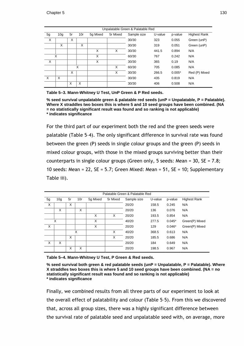
Chapter 5 130
Unpalatable Green & Palatable Red
5g 10g 5r 10r 5g Mixed 5r Mixed Sample size U-value p-value Highest Rank
X X 30/30 323 0.055 Green (unP)
X X 30/30 319 0.051 Green (unP)
X X 30/30 441.5 0.894 N/A
X X 60/30 767 0.242 N/A
X X 30/30 365 0.19 N/A
X X 60/30 705 0.085 N/A
X X 30/30 266.5 0.005* Red (P) Mixed
X X 30/30 435 0.819 N/A
X X 30/30 406 0.508 N/A
Table 5–3. Mann-Whitney U Test, UnP Green & P Red s eeds.
% seed survival unpalatable green & palatable red s eeds (unP = Unpalatable, P = Palatable). Where X straddles two boxes this is where 5 and 10 seed groups have been combined. (NA = no statistically significant result was found and so ranking is not applicable) * indicates significance
For the third part of our experiment both the red and the green seeds were
palatable (Table 5–4). The only significant difference in survival rate was found
between the green (P) seeds in single colour groups and the green (P) seeds in
mixed colour groups, with those in the mixed groups surviving better than their
counterparts in single colour groups (Green only, 5 seeds: Mean = 30, SE = 7.8;
10 seeds: Mean = 22, SE = 5.7; Green Mixed: Mean = 51, SE = 10; Supplementary
Table iii).
Palatable Green & Palatable Red
5g 10g 5r 10r 5g Mixed 5r Mixed Sample size U-value p-value Highest Rank
X X 20/20 158.5 0.245 N/A
X X 20/20 136 0.076 N/A
X X 20/20 193.5 0.854 N/A
X X 40/20 277.5 0.045* Green(P) Mixed
X X 20/20 129 0.046* Green(P) Mixed
X X 40/20 368.5 0.613 N/A
X X 20/20 185.5 0.686 N/A
X X 20/20 184 0.649 N/A
X X 20/20 198.5 0.967 N/A
Table 5–4. Mann-Whitney U Test, P Green & Red seeds .
% seed survival both green & red palatable seeds (u nP = Unpalatable, P = Palatable). Where X straddles two boxes this is where 5 and 10 seed g roups have been combined. (NA = no statistically significant result was found and so r anking is not applicable) * indicates significance
Finally, we combined results from all three parts of our experiment to look at
the overall effect of palatability and colour (Table 5–5). From this we discovered
that, across all group sizes, there was a highly significant difference between
the survival rate of palatable seed and unpalatable seed with, on average, more
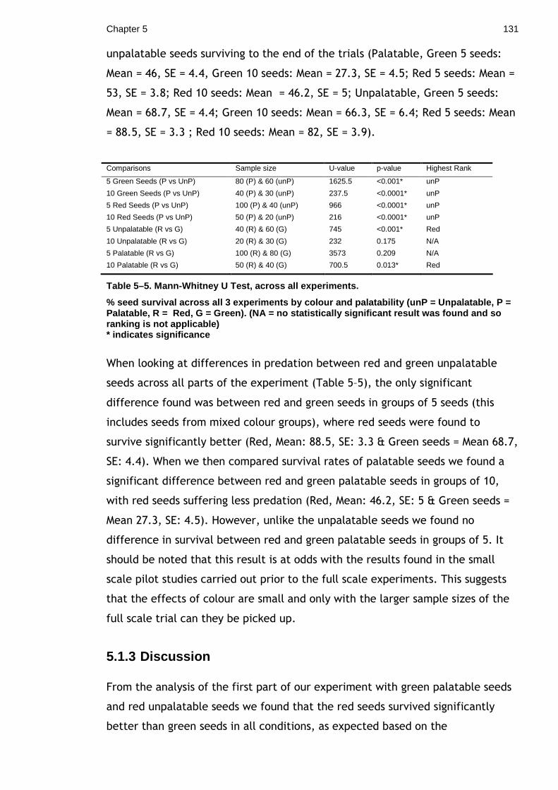
Chapter 5 131
unpalatable seeds surviving to the end of the trials (Palatable, Green 5 seeds:
Mean = 46, SE = 4.4, Green 10 seeds: Mean = 27.3, SE = 4.5; Red 5 seeds: Mean =
53, SE = 3.8; Red 10 seeds: Mean = 46.2, SE = 5; Unpalatable, Green 5 seeds:
Mean = 68.7, SE = 4.4; Green 10 seeds: Mean = 66.3, SE = 6.4; Red 5 seeds: Mean
= 88.5, SE = 3.3 ; Red 10 seeds: Mean = 82, SE = 3.9).
Comparisons Sample size U-value p-value Highest Rank
5 Green Seeds (P vs UnP) 80 (P) & 60 (unP) 1625.5 <0.001* unP
10 Green Seeds (P vs UnP) 40 (P) & 30 (unP) 237.5 <0.0001* unP
5 Red Seeds (P vs UnP) 100 (P) & 40 (unP) 966 <0.0001* unP
10 Red Seeds (P vs UnP) 50 (P) & 20 (unP) 216 <0.0001* unP
5 Unpalatable (R vs G) 40 (R) & 60 (G) 745 <0.001* Red
10 Unpalatable (R vs G) 20 (R) & 30 (G) 232 0.175 N/A
5 Palatable (R vs G) 100 (R) & 80 (G) 3573 0.209 N/A
10 Palatable (R vs G) 50 (R) & 40 (G) 700.5 0.013* Red
Table 5–5. Mann-Whitney U Test, across all experime nts.
% seed survival across all 3 experiments by colour and palatability (unP = Unpalatable, P = Palatable, R = Red, G = Green). (NA = no statistic ally significant result was found and so ranking is not applicable) * indicates significance
When looking at differences in predation between red and green unpalatable
seeds across all parts of the experiment (Table 5–5), the only significant
difference found was between red and green seeds in groups of 5 seeds (this
includes seeds from mixed colour groups), where red seeds were found to
survive significantly better (Red, Mean: 88.5, SE: 3.3 & Green seeds = Mean 68.7,
SE: 4.4). When we then compared survival rates of palatable seeds we found a
significant difference between red and green palatable seeds in groups of 10,
with red seeds suffering less predation (Red, Mean: 46.2, SE: 5 & Green seeds =
Mean 27.3, SE: 4.5). However, unlike the unpalatable seeds we found no
difference in survival between red and green palatable seeds in groups of 5. It
should be noted that this result is at odds with the results found in the small
scale pilot studies carried out prior to the full scale experiments. This suggests
that the effects of colour are small and only with the larger sample sizes of the
full scale trial can they be picked up.
5.1.3 Discussion
From the analysis of the first part of our experiment with green palatable seeds
and red unpalatable seeds we found that the red seeds survived significantly
better than green seeds in all conditions, as expected based on the
Chapter 5 132
unpalatability of the quinine. Moreover, we found that there was a significant
difference in green seed survival between groups, with those in mixed groups
alongside red seeds having a significantly better survival rate than those in
green-only groups. This result supports the “aposematic commensalism”
hypothesis, with the palatable cryptic prey suffering significantly less predation
when grouped together with aposematic neighbours. In comparison, no
difference was found between red seeds in mixed groups and those in red only
groups. This also supports the “aposematic commensalism” hypothesis, as the
added protection the palatable seeds gain apparently does not impose any
corresponding costs on the aposematic seeds they are grouped with.
For the second part of our experiment we investigated how much of the effect
was generated by colour and how much by palatability and, thus, we reversed
the treatment by using green unpalatable seeds and red palatable seeds. Here,
as expected due to the uncoupling of palatability and conspicuous colouring, we
found that the treatment effects were much weaker. Nevertheless, our results
were close to significant (p = 0.055 & 0.051) and might suggest a non-significant
trend in single colour groups with the unpalatable seeds (green) surviving in
greater numbers than the palatable (red) seeds. In this part of the experiment,
no significant difference was found between red and green seed survival in
mixed colour groups, but when red seeds from the single colour groups of 5
seeds were compared with red seeds from mixed groups, it was found that those
grouped with the unpalatable green seeds survived significantly better. This
again supports “aposematic commensalism” and, as in the first part of our
experiment, this demonstrates that there is a benefit for undefended prey to
group with defended prey. However, here, the effect may be weaker when the
unpalatability and aposematic colouring are not tied. In other words, by
combining unpalatability with the classically aposematic colour red(Roper and
Marples, 1997), it is likely there will be a stronger combined aversion than when
combined with the colour green, since many birds have an innate aversion to
red(Mastrota and Mench, 1995).
For the third and final part of our experiment we used groups in which both the
red and green seeds were palatable (). We found that there were no significant
differences in survival for the majority of the comparisons. However, we did find
that the green palatable seed survived significantly better when it was grouped
Chapter 5 133
with red palatable seed. This suggested that, even in the absence of chemical
defences, when in a mixed group of red and green seeds, the green seeds still
appeared to benefit from their proximity to the conspicuous red seeds.
This may be relevant when considering selection pressures on potential Batesian
mimics, with the conspicuous colouring dishonestly signalling unpalatability. In
this case we presented predators with prey groups with no honest signals. We
know that as the ratio of dishonest to honest signals is increased the
effectiveness of the warning signal is reduced and predation rates for both
groups increase(Ruxton et al., 2004). For this experiment we did our best to
minimise learning effects, but we would expect that had we continued
presenting the same predators with groups of all palatable red seeds they would
eventually learn to ignore the red colouration. However, without the time to
learn this, red colouration is still effective in improving the survival rate of
nearby prey, but to a lesser extent than when the conspicuous signal is
supported by chemical defences. Furthermore, these results confirm our
hypothesis that palatable prey can improve their survival rate by grouping with
neighbours that predators may be pre-adapted to interpret as defended.
Finally, we wanted to analyse the effect of colour and unpalatability across all
three parts of the experiment (Table 5–5). We should note that as this analysis
pools the data from the 3 separate experiments conducted between early
autumn and mid-winter, they may be confounded by the time of year. Here we
found that, in all cases, whether coloured red or green, unpalatable seeds had a
greater survival rate than palatable seeds. We found that in groups of palatable
seeds of homogenous colour, red seeds in the larger groups (10 seeds vs. 5)
survived better than green seeds but that there was no difference in the smaller
groups. This might suggest that, where the aposematic signal is dishonest, it
takes the greater stimulus of a larger group and a greater area of warning
colouration to illicit a reaction from predators, which confirms an effect found
in previous studies(Gamberale and Tullberg, 1998).
We had expected that, when looking at the unpalatable seeds, in those cases
where seeds were both red (warning coloured) and unpalatable, these seeds
would survive better than unpalatable green seeds. What we found, however,
was that only in the groups of 5 seeds did red seeds survive significantly better
Chapter 5 134
than green. We are unsure as to why this was not the case for the groups of 10
seeds but it may be that this is a product of the smaller sample size obtained for
the 10 seed groups. In summary, our results show that (1) undefended non-
aposematic prey can benefit by grouping with aposematic and defended prey
and that (2) there is no evidence that the aposematic prey suffered greater
predation by their association with the palatable prey.
It is important to take protection by association or ‘aposematic commensalism’
in to account when talking about the evolution of aposematic signals. Is this an
effect of proximity? Perhaps predators avoid locations where they have had
noxious experiences, with all prey within a certain distance lumped together and
avoided? Or perhaps, rather than proximity in space, should we consider
proximity in time, with unpalatable prey or an aversive experience causing a
period of disinterest in food, of any kind? This could be tested by providing
distasteful prey within a test area and observing whether there is any latency to
the selection of further prey items and if this changed by moving to a new test
area. We might also want to investigate what cues are being used; are they
purely visual or might odour be playing some part? We know that odour can be
used in conjunction with colour to advertise unprofitability(Kelly and Marples,
2004), and, with the effects of wind, dispersal odour cues are likely to have a
much less defined effective area than that of colour. This may mean that
neighbouring undefended prey can benefit from aversive odour cues emitted by
others by grouping with them. The prey items we used were very different in
colour. In all other ways, such as size and shape, they were very similar. Had we
had used palatable prey that were different in those aspects, would they still
have benefited from their aposematic neighbours?
We speculate that it would be of particular relevance to the evolution of
aposematic colouring if we were to find that these benefits could cross
kingdoms, with palatable animals able to benefit by grouping with unpalatable
plants or vice versa. It is thought that some defended plants use aposematic
signals similar to animals(Inbar et al., ; Lev-Yadun, 2009; Rubino and McCarthy).
If animals were able to benefit by association with these plant species and vice
versa, it might help to explain the convergence of signals between these very
different groups. We might also consider that warning signals might have first
Chapter 5 135
evolved within plants, with animals, later, co-opting an already established
system by close association with defended plant species.
A similar phenomenon to the one we describe here has been also been found in
plants with the discovery of ‘magnet species’(Molina-Montenegro et al., 2008). It
was found that species with flowers that were less attractive or profitable to
pollinators were able to increase pollination and their seed production by
associating with more attractive species. This, along with our results, leads us to
speculate that perhaps this type of commensal relationship may be
comparatively common within the natural world.
Our results may also point to potential consequences for the evolution of
Batesian mimicry. One of the biggest questions on mimicry that remains to be
answered is how a species can survive through the intermediate stages of
evolving a conspicuous display. Assuming an undefended species initially begins
with cryptic patterning, there is presumably a point at which they are neither
fully cryptic nor conspicuous and therefore at very high risk of predation (being
both easily visible and undefended). We speculate that if such a species was
able to reduce their predation rate by associating closely with their defended
model, they may be able to survive long enough to evolve a better mimicry.
Eventually, increasingly more accurate mimicry could free them to associate less
closely with their models. However, the mechanism explored here may also act
to reduce the likelihood of Batesian mimicry evolving, because the anti-
predatory advantage of close association without mimicry may reduce the fitness
advantage of changing appearance towards mimicry, particularly where the
model and mimic closely share habitat requirements. To properly examine this
we will need to carry out further experiments to examine how differing levels of
mimicry affect fitness.
The results shown here suggest that a full understanding of selection pressures
associated with mimicry requires consideration of the benefits of close
association without mimicry. Although mimicry has been closely studied because
of its evolutionary significance most prey species do not evolve to be Batesian
mimics and the aposematic commensalism highlighted here may be an important
but hitherto neglected factor in explaining this phenomenon.
General Discussion 136
General Discussion
Using both field and lab experiments I have examined adaptations that reduce
predation rate and in particular how colouration and patterning reduce risk of
predation, both as a single organism or as part of a group when against the
natural environment. While each of the strategies I have examined are
important in their own right, it is however important to realise that they do not
occur in isolation and they are often encountered simultaneously, either as part
of a community or within the same animal and so their effects are likely to be
modified. I also did not consider the genetic basis of the traits I studied and any
constraints here may have considerable effects on the evolution of anti-predator
strategies. Gene studies are also extremely useful in examining the origins of an
adaptation and our understanding of how they spread throughout a population.
For example some recent work examining the mimetic history of the Heliconius
butterflies has redefined our understanding of their colour pattern evolution.
Previous studies using neutral markers (not linked to the colour pattern loci)
suggested that similar colour patterns had arisen independently, multiple times,
in each species with populations partitioned by geographic region. However, this
most recent study used markers linked to the colour pattern loci and a gene
which controls red colour pattern variation. The results of this approach
suggested a single origin of the pattern element within each species and
demonstrated the importance of using markers from the phenotypic-determining
genomic region to understand the evolutionary history of an adaptive trait(Hines
et al.).
Symmetry of body plan is something common to most complex organisms and
may be to some extent a constraint on the types of patterning an organism can
evolve. In chapters 1 and 2 I examined aspects of cryptic and aposematic
patterning, both of which have been studied in respect to the effect of
symmetry on their anti-predator effects. In chapter 1 I found that asymmetry
has no effect on predation rate, a result that is in agreement with other recent
studies. However, we must still find a way to marry these findings with
symmetry studies that have found symmetrical patterns are more easily
detected, learnt and reproduced. These two set of results seem to be
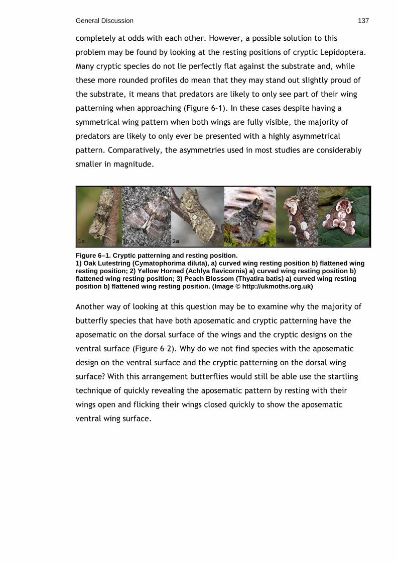
General Discussion 137
completely at odds with each other. However, a possible solution to this
problem may be found by looking at the resting positions of cryptic Lepidoptera.
Many cryptic species do not lie perfectly flat against the substrate and, while
these more rounded profiles do mean that they may stand out slightly proud of
the substrate, it means that predators are likely to only see part of their wing
patterning when approaching (Figure 6–1). In these cases despite having a
symmetrical wing pattern when both wings are fully visible, the majority of
predators are likely to only ever be presented with a highly asymmetrical
pattern. Comparatively, the asymmetries used in most studies are considerably
smaller in magnitude.
Figure 6–1. Cryptic patterning and resting position . 1) Oak Lutestring (Cymatophorima diluta), a) curved wing resting position b) flattened wing resting position; 2) Yellow Horned (Achlya flavicor nis) a) curved wing resting position b) flattened wing resting position; 3) Peach Blossom ( Thyatira batis) a) curved wing resting position b) flattened wing resting position. (Image © http://ukmoths.org.uk)
Another way of looking at this question may be to examine why the majority of
butterfly species that have both aposematic and cryptic patterning have the
aposematic on the dorsal surface of the wings and the cryptic designs on the
ventral surface (Figure 6–2). Why do we not find species with the aposematic
design on the ventral surface and the cryptic patterning on the dorsal wing
surface? With this arrangement butterflies would still be able use the startling
technique of quickly revealing the aposematic pattern by resting with their
wings open and flicking their wings closed quickly to show the aposematic
ventral wing surface.
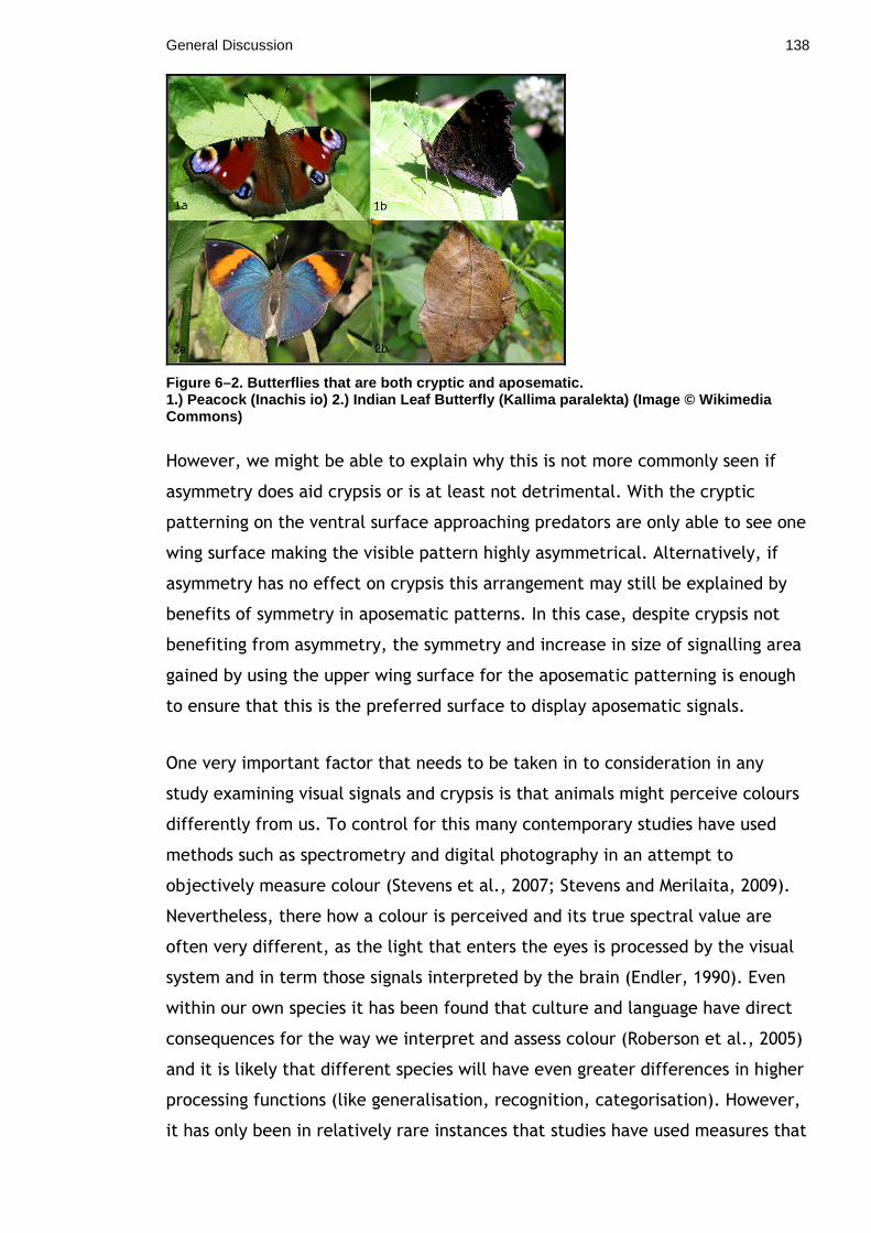
General Discussion 138
Figure 6–2. Butterflies that are both cryptic and a posematic. 1.) Peacock ( Inachis io) 2.) Indian Leaf Butterfly ( Kallima paralekta) (Image © Wikimedia Commons)
However, we might be able to explain why this is not more commonly seen if
asymmetry does aid crypsis or is at least not detrimental. With the cryptic
patterning on the ventral surface approaching predators are only able to see one
wing surface making the visible pattern highly asymmetrical. Alternatively, if
asymmetry has no effect on crypsis this arrangement may still be explained by
benefits of symmetry in aposematic patterns. In this case, despite crypsis not
benefiting from asymmetry, the symmetry and increase in size of signalling area
gained by using the upper wing surface for the aposematic patterning is enough
to ensure that this is the preferred surface to display aposematic signals.
One very important factor that needs to be taken in to consideration in any
study examining visual signals and crypsis is that animals might perceive colours
differently from us. To control for this many contemporary studies have used
methods such as spectrometry and digital photography in an attempt to
objectively measure colour (Stevens et al., 2007; Stevens and Merilaita, 2009).
Nevertheless, there how a colour is perceived and its true spectral value are
often very different, as the light that enters the eyes is processed by the visual
system and in term those signals interpreted by the brain (Endler, 1990). Even
within our own species it has been found that culture and language have direct
consequences for the way we interpret and assess colour (Roberson et al., 2005)
and it is likely that different species will have even greater differences in higher
processing functions (like generalisation, recognition, categorisation). However,
it has only been in relatively rare instances that studies have used measures that

General Discussion 139
relate directly to the visual processing of the receiver (Cassey et al., 2008;
Hastad et al., 2005; Langmore et al., 2009; Lovell et al., 2005; Stevens and
Cuthill, 2006; Tanaka et al., 2011)
Taking all this into account, I hope I have demonstrated that there still are many
fascinating questions left to explore in the field of visual anti-predator
adaptations. However, future work should (i) take predator physiology and
psychology into account, (ii) look at trade-offs between functions, (iii) look at
developmental (iv) and genetic constraints
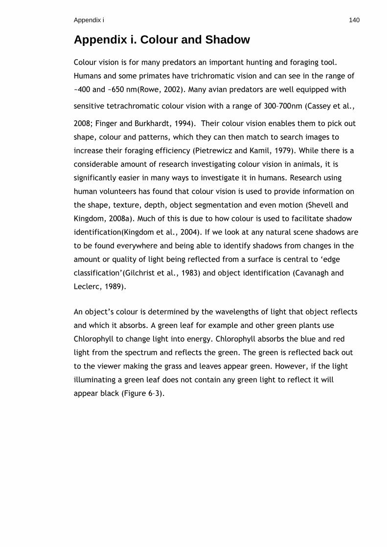
Appendix i 140
Appendix i. Colour and Shadow
Colour vision is for many predators an important hunting and foraging tool.
Humans and some primates have trichromatic vision and can see in the range of
~400 and ~650 nm(Rowe, 2002). Many avian predators are well equipped with
sensitive tetrachromatic colour vision with a range of 300–700 nm (Cassey et al.,
2008; Finger and Burkhardt, 1994). Their colour vision enables them to pick out
shape, colour and patterns, which they can then match to search images to
increase their foraging efficiency (Pietrewicz and Kamil, 1979). While there is a
considerable amount of research investigating colour vision in animals, it is
significantly easier in many ways to investigate it in humans. Research using
human volunteers has found that colour vision is used to provide information on
the shape, texture, depth, object segmentation and even motion (Shevell and
Kingdom, 2008a). Much of this is due to how colour is used to facilitate shadow
identification(Kingdom et al., 2004). If we look at any natural scene shadows are
to be found everywhere and being able to identify shadows from changes in the
amount or quality of light being reflected from a surface is central to ‘edge
classification’(Gilchrist et al., 1983) and object identification (Cavanagh and
Leclerc, 1989).
An object’s colour is determined by the wavelengths of light that object reflects
and which it absorbs. A green leaf for example and other green plants use
Chlorophyll to change light into energy. Chlorophyll absorbs the blue and red
light from the spectrum and reflects the green. The green is reflected back out
to the viewer making the grass and leaves appear green. However, if the light
illuminating a green leaf does not contain any green light to reflect it will
appear black (Figure 6–3).
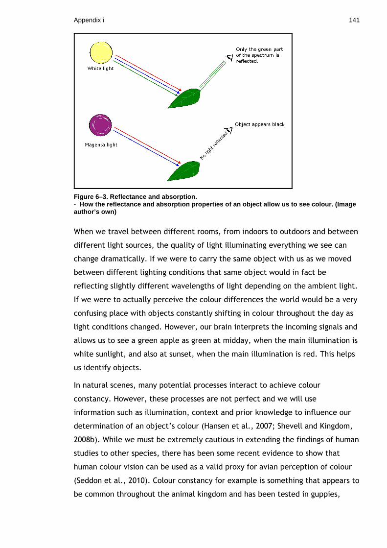
Appendix i 141
Figure 6–3. Reflectance and absorption. - How the reflectance and absorption properties of an object allow us to see colour. (Image author’s own)
When we travel between different rooms, from indoors to outdoors and between
different light sources, the quality of light illuminating everything we see can
change dramatically. If we were to carry the same object with us as we moved
between different lighting conditions that same object would in fact be
reflecting slightly different wavelengths of light depending on the ambient light.
If we were to actually perceive the colour differences the world would be a very
confusing place with objects constantly shifting in colour throughout the day as
light conditions changed. However, our brain interprets the incoming signals and
allows us to see a green apple as green at midday, when the main illumination is
white sunlight, and also at sunset, when the main illumination is red. This helps
us identify objects.
In natural scenes, many potential processes interact to achieve colour
constancy. However, these processes are not perfect and we will use
information such as illumination, context and prior knowledge to influence our
determination of an object’s colour (Hansen et al., 2007; Shevell and Kingdom,
2008b). While we must be extremely cautious in extending the findings of human
studies to other species, there has been some recent evidence to show that
human colour vision can be used as a valid proxy for avian perception of colour
(Seddon et al., 2010). Colour constancy for example is something that appears to
be common throughout the animal kingdom and has been tested in guppies,
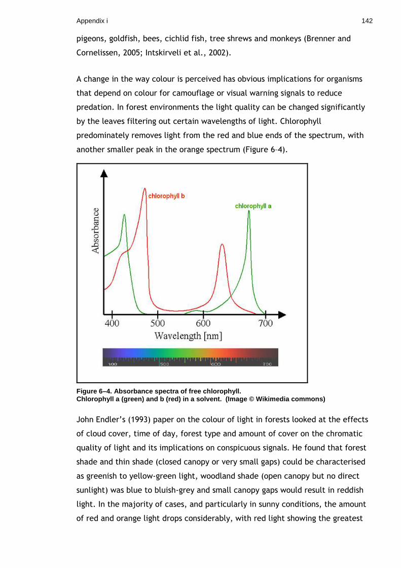
Appendix i 142
pigeons, goldfish, bees, cichlid fish, tree shrews and monkeys (Brenner and
Cornelissen, 2005; Intskirveli et al., 2002).
A change in the way colour is perceived has obvious implications for organisms
that depend on colour for camouflage or visual warning signals to reduce
predation. In forest environments the light quality can be changed significantly
by the leaves filtering out certain wavelengths of light. Chlorophyll
predominately removes light from the red and blue ends of the spectrum, with
another smaller peak in the orange spectrum (Figure 6–4).
Figure 6–4. Absorbance spectra of free chlorophyll. Chlorophyll a (green) and b (red) in a solvent. (I mage © Wikimedia commons)
John Endler’s (1993) paper on the colour of light in forests looked at the effects
of cloud cover, time of day, forest type and amount of cover on the chromatic
quality of light and its implications on conspicuous signals. He found that forest
shade and thin shade (closed canopy or very small gaps) could be characterised
as greenish to yellow-green light, woodland shade (open canopy but no direct
sunlight) was blue to bluish-grey and small canopy gaps would result in reddish
light. In the majority of cases, and particularly in sunny conditions, the amount
of red and orange light drops considerably, with red light showing the greatest
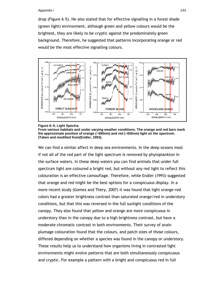
Appendix i 143
drop (Figure 6–5). He also stated that for effective signalling in a forest shade
(green light) environment, although green and yellow colours would be the
brightest, they are likely to be cryptic against the predominately green
background. Therefore, he suggested that patterns incorporating orange or red
would be the most effective signalling colours.
Figure 6–5. Light Spectra. From various habitats and under varying weather con ditions. The orange and red bars mark the approximate position of orange (~590nm) and red (~650nm) light on the spectrum. (Taken and modified from(Endler, 1993).
We can find a similar affect in deep sea environments. In the deep oceans most
if not all of the red part of the light spectrum is removed by phytoplankton in
the surface waters. In these deep waters you can find animals that under full
spectrum light are coloured a bright red, but without any red light to reflect this
colouration is an effective camouflage. Therefore, while Endler (1993) suggested
that orange and red might be the best options for a conspicuous display. In a
more recent study (Gomez and Thery, 2007) it was found that light orange-red
colors had a greater brightness contrast than saturated orange/red in understory
conditions, but that this was reversed in the full sunlight conditions of the
canopy. They also found that yellow and orange are more conspicuous in
understory than in the canopy due to a high brightness contrast, but have a
moderate chromatic contrast in both environments. Their survey of avain
plumage colouration found that the colours, and patch sizes of those colours,
differed depending on whether a species was found in the canopy or understory.
These results help us to understand how organisms living in contrasted light
environments might evolve patterns that are both simultaneously conspicuous
and cryptic. For example a pattern with a bright and conspicuous red in full
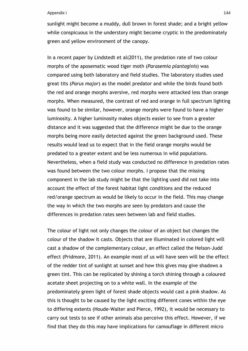
Appendix i 144
sunlight might become a muddy, dull brown in forest shade; and a bright yellow
while conspicuous in the understory might become cryptic in the predominately
green and yellow environment of the canopy.
In a recent paper by Lindstedt et al(2011), the predation rate of two colour
morphs of the aposematic wood tiger moth (Parasemia plantaginis) was
compared using both laboratory and field studies. The laboratory studies used
great tits (Parus major) as the model predator and while the birds found both
the red and orange morphs aversive, red morphs were attacked less than orange
morphs. When measured, the contrast of red and orange in full spectrum lighting
was found to be similar, however, orange morphs were found to have a higher
luminosity. A higher luminosity makes objects easier to see from a greater
distance and it was suggested that the difference might be due to the orange
morphs being more easily detected against the green background used. These
results would lead us to expect that in the field orange morphs would be
predated to a greater extent and be less numerous in wild populations.
Nevertheless, when a field study was conducted no difference in predation rates
was found between the two colour morphs. I propose that the missing
component in the lab study might be that the lighting used did not take into
account the effect of the forest habitat light conditions and the reduced
red/orange spectrum as would be likely to occur in the field. This may change
the way in which the two morphs are seen by predators and cause the
differences in predation rates seen between lab and field studies.
The colour of light not only changes the colour of an object but changes the
colour of the shadow it casts. Objects that are illuminated in colored light will
cast a shadow of the complementary colour, an effect called the Helson-Judd
effect (Pridmore, 2011). An example most of us will have seen will be the effect
of the redder tint of sunlight at sunset and how this gives may give shadows a
green tint. This can be replicated by shining a torch shining through a coloured
acetate sheet projecting on to a white wall. In the example of the
predominately green light of forest shade objects would cast a pink shadow. As
this is thought to be caused by the light exciting different cones within the eye
to differing extents (Houde-Walter and Pierce, 1992), it would be necessary to
carry out tests to see if other animals also perceive this effect. However, if we
find that they do this may have implications for camouflage in different micro
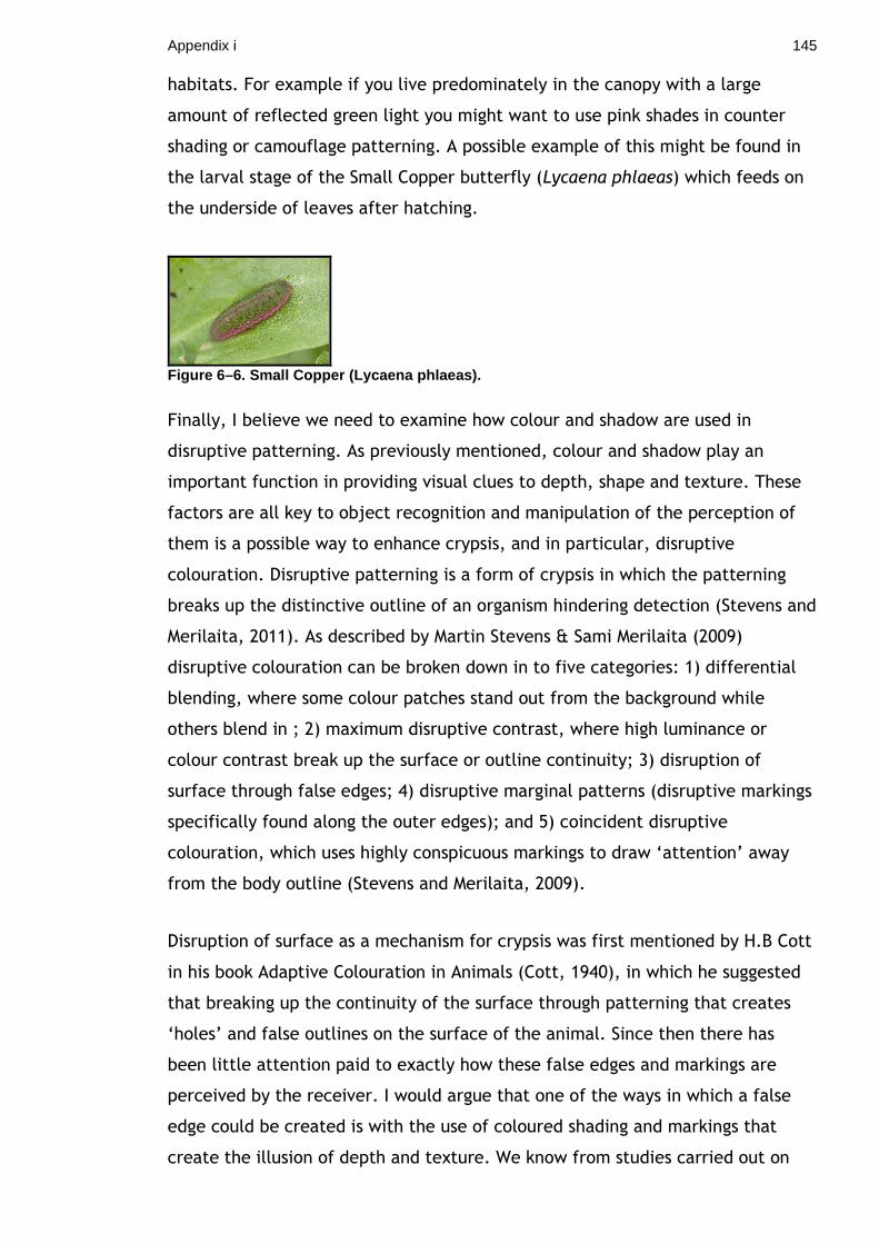
Appendix i 145
habitats. For example if you live predominately in the canopy with a large
amount of reflected green light you might want to use pink shades in counter
shading or camouflage patterning. A possible example of this might be found in
the larval stage of the Small Copper butterfly (Lycaena phlaeas) which feeds on
the underside of leaves after hatching.
Figure 6–6. Small Copper ( Lycaena phlaeas).
Finally, I believe we need to examine how colour and shadow are used in
disruptive patterning. As previously mentioned, colour and shadow play an
important function in providing visual clues to depth, shape and texture. These
factors are all key to object recognition and manipulation of the perception of
them is a possible way to enhance crypsis, and in particular, disruptive
colouration. Disruptive patterning is a form of crypsis in which the patterning
breaks up the distinctive outline of an organism hindering detection (Stevens and
Merilaita, 2011). As described by Martin Stevens & Sami Merilaita (2009)
disruptive colouration can be broken down in to five categories: 1) differential
blending, where some colour patches stand out from the background while
others blend in ; 2) maximum disruptive contrast, where high luminance or
colour contrast break up the surface or outline continuity; 3) disruption of
surface through false edges; 4) disruptive marginal patterns (disruptive markings
specifically found along the outer edges); and 5) coincident disruptive
colouration, which uses highly conspicuous markings to draw ‘attention’ away
from the body outline (Stevens and Merilaita, 2009).
Disruption of surface as a mechanism for crypsis was first mentioned by H.B Cott
in his book Adaptive Colouration in Animals (Cott, 1940), in which he suggested
that breaking up the continuity of the surface through patterning that creates
‘holes’ and false outlines on the surface of the animal. Since then there has
been little attention paid to exactly how these false edges and markings are
perceived by the receiver. I would argue that one of the ways in which a false
edge could be created is with the use of coloured shading and markings that
create the illusion of depth and texture. We know from studies carried out on
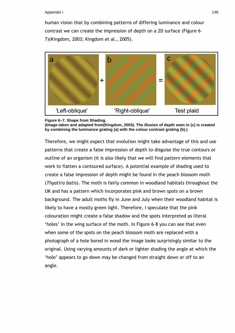
Appendix i 146
human vision that by combining patterns of differing luminance and colour
contrast we can create the impression of depth on a 2D surface (Figure 6–
7)(Kingdom, 2003; Kingdom et al., 2005).
Figure 6–7. Shape from Shading. (Image taken and adapted from(Kingdom, 2003). The i llusion of depth seen in (c) is created by combining the luminance grating (a) with the col our contrast grating (b).)
Therefore, we might expect that evolution might take advantage of this and use
patterns that create a false impression of depth to disguise the true contours or
outline of an organism (it is also likely that we will find pattern elements that
work to flatten a contoured surface). A potential example of shading used to
create a false impression of depth might be found in the peach blossom moth
(Thyatira batis). The moth is fairly common in woodland habitats throughout the
UK and has a pattern which incorporates pink and brown spots on a brown
background. The adult moths fly in June and July when their woodland habitat is
likely to have a mostly green light. Therefore, I speculate that the pink
colouration might create a false shadow and the spots interpreted as literal
‘holes’ in the wing surface of the moth. In Figure 6–8 you can see that even
when some of the spots on the peach blossom moth are replaced with a
photograph of a hole bored in wood the image looks surprisingly similar to the
original. Using varying amounts of dark or lighter shading the angle at which the
‘hole’ appears to go down may be changed from straight down or off to an
angle.
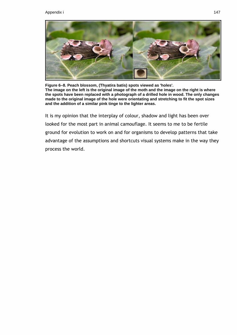
Appendix i 147
Figure 6–8. Peach blossom, ( Thyatira batis) spots viewed as 'holes'. The image on the left is the original image of the moth and the image on the right is where the spots have been replaced with a photograph of a drilled hole in wood. The only changes made to the original image of the hole were orienta ting and stretching to fit the spot sizes and the addition of a similar pink tinge to the lig hter areas.
It is my opinion that the interplay of colour, shadow and light has been over
looked for the most part in animal camouflage. It seems to me to be fertile
ground for evolution to work on and for organisms to develop patterns that take
advantage of the assumptions and shortcuts visual systems make in the way they
process the world.
Appendix ii 148
Appendix ii. Comparison of Eyespot experimental techniques and methodologies
Jones, 1980 & Stevens et al, 2007, 2008 a, 2009a.
Both Jones and Stevens et al carried out similar experiments with the aim of
examining predator avoidance of eye-spots and in particular what attributes
cause these reactions i.e. is the reaction elicited due to their similarity to eyes
or due to their conspicuous colouration? Despite many similarities in their
approach these experiments produced two opposing conclusions; with Stevens et
al concluding that conspicuousness is the determining factor and Jones that eye
mimicry is integral. Here I examine both experiments in an attempt to find
possible explanations for such differing opinions.
The basic experimental setup for both Stevens and Jones was similar, with both
using avian predators and cardboard stimuli bearing shapes designed to be more
or less eye-like in their appearance. However, while Jones chose a lab based
system with naïve male domesticated chicks, Stevens used a field setup and an
assemblage of wild birds. It is this choice of field over lab setup which
introduces many of the differences between the two sets of experiments. In
particular the use of captive chicks greatly reduced the number of replicates
that Jones could carry out.
Jones produced their stimuli using plain white card with the test patterns
marked in indelible black ink bordered by a basic representation of a head and
beak. The stimuli were introduced to the chicks from a maximum distance of
680mm (the length of the box in which they were housed). Stevens used printed
card with a background colour intended to be half-way between black and
white, with the stimuli pinned to trees at a height of 1-3m. The average distance
at which they were first encountered is likely to have varied considerably, but
we can assume that on average the stimuli were likely to be seen from some
distance before being approached. This may have affected the way in which the
stimuli were perceived particularly, as pointed out by Stevens, the diamond (or
square?) stimuli may look similar to the circular stimuli from a distance.
Appendix ii 149
The criteria to determine what effect the stimuli have had differs considerably
between the experiments, with Jones using behavioural cues such as freezing,
avoidance, distress and number of steps or jumps of the test chick. Conversely
Stevens et al used the removal of a bait attached to the stimulus as an
indication of how effective the stimulus was at inducing predator avoidance
(with baits removed by non-avian predators discounted).
Overall, both approaches have their strengths and weaknesses with the lab
experiments providing greater control and observational opportunities, but
lacking in realism and the field studies limiting our ability to observe the way
the stimuli are approached and treated by predators, but allowing the stimuli to
be selected by the predator community rather than one individual.
A compromise perhaps between the two that might enable us to use the best
aspects of both techniques may be an aviary study using wild birds. This would
allow greater opportunities to observe predation as it occurs, but in a more
natural setting.
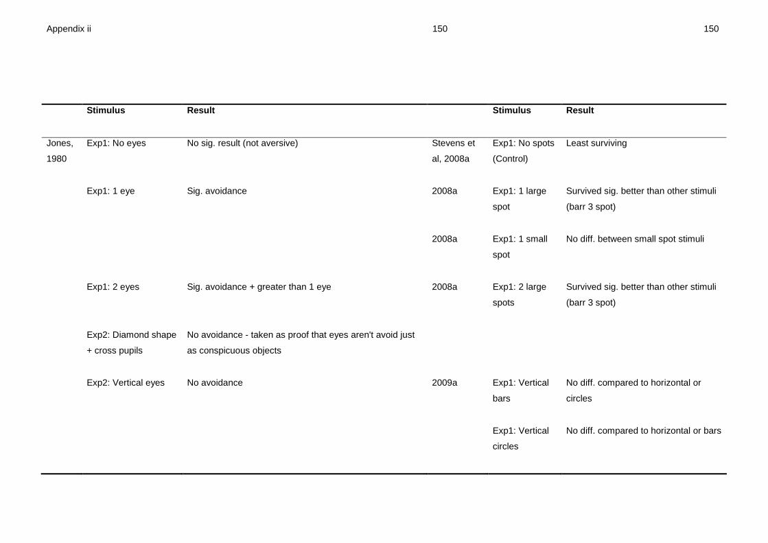
Appendix ii 150 150
Stimulus Result Stimulus Result
Jones,
1980
Exp1: No eyes No sig. result (not aversive) Stevens et
al, 2008a
Exp1: No spots
(Control)
Least surviving
Exp1: 1 eye Sig. avoidance 2008a Exp1: 1 large
spot
Survived sig. better than other stimuli
(barr 3 spot)
2008a Exp1: 1 small
spot
No diff. between small spot stimuli
Exp1: 2 eyes Sig. avoidance + greater than 1 eye 2008a Exp1: 2 large
spots
Survived sig. better than other stimuli
(barr 3 spot)
Exp2: Diamond shape
+ cross pupils
No avoidance - taken as proof that eyes aren't avoid just
as conspicuous objects
Exp2: Vertical eyes No avoidance 2009a Exp1: Vertical
bars
No diff. compared to horizontal or
circles
Exp1: Vertical
circles
No diff. compared to horizontal or bars
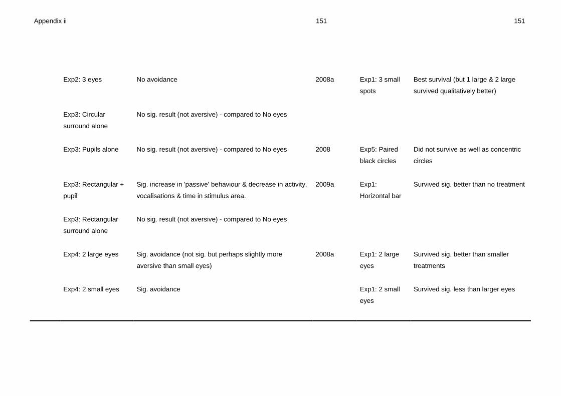
Appendix ii 151 151
Exp2: 3 eyes No avoidance 2008a Exp1: 3 small
spots
Best survival (but 1 large & 2 large
survived qualitatively better)
Exp3: Circular
surround alone
No sig. result (not aversive) - compared to No eyes
Exp3: Pupils alone No sig. result (not aversive) - compared to No eyes 2008 Exp5: Paired
black circles
Did not survive as well as concentric
circles
Exp3: Rectangular +
pupil
Sig. increase in 'passive' behaviour & decrease in activity,
vocalisations & time in stimulus area.
2009a Exp1:
Horizontal bar
Survived sig. better than no treatment
Exp3: Rectangular
surround alone
No sig. result (not aversive) - compared to No eyes
Exp4: 2 large eyes Sig. avoidance (not sig. but perhaps slightly more
aversive than small eyes)
2008a Exp1: 2 large
eyes
Survived sig. better than smaller
treatments
Exp4: 2 small eyes Sig. avoidance Exp1: 2 small
eyes
Survived sig. less than larger eyes

Appendix iii 152
Appendix iii. British Caterpillar Database
This database was intended to catalogue the physical characteristics of
approximately 864 British caterpillars. The main sources of data used were The
colour identification guide to: Caterpillars of the British Isles by Jim Porter
(Porter, 1997) and A field guide to caterpillars of Britain and Europe by David J.
Carter(Carter and Hargreaves, 1986).
The purpose of compiling this database was to use the information to investigate
the relationship between aposematic colouration, physical characteristics and
life history traits.
To do this I collated data on these physical attributes:
1. The instar being described 2. Colour: Background colour, Head colour, Colour patterns (stripes, spots, etc)
Countershading, Cryptic, Aposematic or Masquerade 3. Hair 4. Body shape & texture 5. Body size And these life cycle attributes:
1. Number of broods e.g. Univoltine/Bivoltine 2. Month of pupation, emergence and laying 3. Are eggs laid eggs laid singly, in groups or scattered 4. Life span 5. Pupation site 6. Over-wintering stage e.g. adult, pupa, etc 7. If larvae are known to be diurnal/nocturnal/corpuscular 8. Gregariousness
The data collected was used in the paper:
Higginson AD, de Wert L, Rowland HM, Ruxton GD, Speed MP (in press) Masquerade is
associated with polyphagy and larval overwintering in the Lepidoptera. Biological Journal of the
Linnean Society

Supplementary Materials 153
Supplementary Materials
Green (P)Groups Before After Red (UnP) Groups Before After 1 10 0 1 10 8 2 10 8 2 10 10 3 10 0 3 10 10 4 10 8 4 10 9 5 10 0 5 10 6
Total 50 16 Total 50 43
Supplementary Table i. Pilot Results *Mann-Whitney U test: U-value = 3.000, P-value = 0. 056
Groups Average Surviving Day 1 6x 10 Palatable Green seeds 3.2 6x 10 Palatable Red seeds 3.3 Day 2 5x 10 Unpalatable Green seeds 6.4 6x 10 Unpalatable Red seeds 7.2
Supplementary Table ii. Small scale test results. *Anova test of colour: p-value = 0.803
Group type 5 seeds 10 seeds Mixed 5&5 Experiment 1 Average % Red Survival (UnP) 89.0 82.0 88.0 SD 17.7 17.4 23.8 SE 4.0 3.9 5.3 Average % Green Survival (P) 29.0 32.5 74.0 SD 32.1 30.9 26.8 SE 7.2 6.9 6.0 Experiment 2 Average % Red Survival (P) 44.7 49.3 71.3 SD 35.9 36.7 33.9 SE 6.6 6.7 6.2 Average % Green Survival (UnP) 64.0 66.3 73.3 SD 35.8 34.8 32.9 SE 6.5 6.4 6.0 Experiment 3 Average % Red Survival (P) 42.0 41.5 49.0 SD 34.9 34.4 44.7 SE 7.7 7.7 10.0 Average % Green Survival (P) 30.0 22.0 51.0 SD 34.6 25.7 44.7 SE 7.8 5.7 10.0
Supplementary Table iii. Average % of seeds survivi ng per Group, per treatment (unP = Unpalatable, P = Palatable.)

Supplementary Materials 154
Supplementary Figure 1. Predator Game Instructions
Supplementary Figure 2. Non-predator Game Instructi ons
List of References 155
List of References
2012. Butterfly Conservation. National Biodiversity Network's Gateway. http://data.nbn.org.uk/interactive/map.jsp?srchSp=NBNSYS0000005724
Allen JA, Raison HE, Weale ME, 1998. The influence of density on frequency-dependent selection by wild birds feeding on artificial prey. Proceedings of the Royal Society of London Series B-Biological Sciences 265:1031-1035.
Allen JA, Weale ME, 2005. Anti-apostatic selection by wild birds on quasi-natural morphs of the land snail Cepaea hortensis: a generalised linear mixed models approach. Oikos 108:335-343.
Almany GR, Peacock LF, Syms C, McCormick MI, Jones GP, 2006. Predators target rare prey in coral reef fish assemblages. Oecologia (Berlin) 152:751-761.
Almany GR, Webster MS, 2004. Odd species out as predators reduce diversity of coral-reef fishes. Ecology 85:2933-2937.
Attneave F, 1954. Some informational aspects of visual perception. Psychological Review 61:183-193.
Bateson M, Nettle D, Roberts G, 2006. Cues of being watched enhance cooperation in a real-world setting. Biol Lett 2:412-414.
Baumgart W, 2011. In the "pursuit distance flight" 400-500 km/h are for many types of peregrine Falco peregrinus normality. Ornithologische Mitteilungen 63:208-225.
Bedford GO, 1978. Biology and ecology of the Phasmatodea. In: Mittler, Thomas E, Carroll N Smith and Vincent H Resh; 125-149.
Blest AD, 1957. The function of eyespot patterns in the Lepidoptera. Behaviour, Leiden 11:209-256.
Brenner E, Cornelissen FW, 2005. A way of selectively degrading colour constancy demonstrates the experience dependence of colour vision. Curr Biol 15:R864-R866.
Broom M, Ruxton GD, 2005. You can run - or you can hide: optimal strategies for cryptic prey against pursuit predators. Behav Ecol 16:534-540.
Brower AVZ, 1996. Parallel race formation and the evolution of mimicry in Heliconius butterflies: A phylogenetic hypothesis from mitochondrial DNA sequences. Evolution 50:195-221.
Bugnyar T, Stowe M, Heinrich B, 2004. Ravens, Corvus corax, follow gaze direction of humans around obstacles. Proceedings of the Royal Society of London Series B-Biological Sciences 271:1331-1336.
Burger J, Gochfeld M, Murray BG, 1991. Role of predators eye size in risk perception by basking black iguana, Ctenosaura-similis. Anim Behav 42:471-476.
Carr JM, Lima SL, 2010. High wind speeds decrease the responsiveness of birds to potentially threatening moving stimuli. Anim Behav 80:215-220.
Carter DJ, Hargreaves B, 1986. A field guide to caterpillars of butterflies and moths in Britain and Europe. In: A field guide to caterpillars of butterflies and moths in Britain and Europe: Collins, London; 1-296.
Carter J, Lyons NJ, Cole HL, Goldsmith AR, 2008. Subtle cues of predation risk: starlings respond to a predator's direction of eye-gaze. Proc R Soc B-Biol Sci 275:1709-1715.
Cassey P, Honza M, Grim T, Hauber ME, 2008. The modelling of avian visual perception predicts behavioural rejection responses to foreign egg colours. Biol Lett 4:515-517.
Cavanagh P, Leclerc YG, 1989. Shape from Shadows. J Exp Psychol-Hum Percept Perform 15:3-27.
List of References 156
Ciuti S, Apollonio M, 2011. Do Antlers Honestly Advertise the Phenotypic Quality of Fallow Buck (Dama dama) in a Lekking Population? Ethology 117:133-144.
Conty L, Gimmig D, Belletier C, George N, Huguet P, 2010. The cost of being watched: Stroop interference increases under concomitant eye contact. Cognition 115:133-139.
Coppinger RP, 1969. Effect of experience and novelty on avian feeding behaviour with reference to evolution of warning colouration in butterflies. Part: 1 Reactions of wild-caught adult blue jays to novel insects. Behaviour 35:45-&.
Coppinger RP, 1970. Effect of experience and novelty on avian feeding behaviour with reference to evolution of warning colouration in butterflies. Part :2 Reactions of naive birds to novel insects. American Naturalist 104:323-&.
Coss RG, 1978. Perceptual determinants of gaze aversion by lesser mouse lemur (Microcebus-murinus), role of 2 facing eyes. Behaviour 64:249-&.
Coss RG, 1979. Delayed plasticity of an instinct - Recognition and avoidance of 2 facing eyes by the jewel fish. Developmental Psychobiology 12:335-345.
Cott HB, 1940. Adaptive coloration in animals. In: Adaptive coloration in animal: Oxford University Press; xxxii + 508p. Col. frontispiece, 548 pl., 584 fig.
Cox DR, 1972. Regression models and life-tables. Journal of the Royal Statistical Society Series B-Statistical Methodology 34:187-&.
Cuthill IC, Hiby E, Lloyd E, 2006a. The predation costs of symmetrical cryptic coloration. Proc R Soc B-Biol Sci 273:1267-1271.
Cuthill IC, Stevens M, Sheppard J, Maddocks T, Parraga CA, Troscianko TS, 2005. Disruptive coloration and background pattern matching. Nature 434:72-74.
Cuthill IC, Stevens M, Windsor AMM, Walker HJ, 2006b. The effects of pattern symmetry on detection of disruptive and background-matching coloration. Behav Ecol 17:828-832.
Dawkins R, 1976. The Selfish Gene. Oxford: Oxford University Press. Dawkins R, 1996. Climbing Mount Improbable. London: Viking. de Ruiter L, 1952. Some Experiments on the Camouflage of Stick Caterpillars.
Behaviour 4:222-232. Delius JD, Nowak B, 1982. Visual symmetry recognition by pigeons. Psychological
Research-Psychologische Forschung 44:199-212. Dittrich L, Rose J, Buschmann JUF, Bourdonnais M, Gunturkun O, 2010. Peck
tracking: a method for localizing critical features within complex pictures for pigeons. Animal Cognition 13:133-143.
Dockery M, Meneely J, Costen P, 2009. Avoiding detection by predators: the tactics used by Biston betularia larvae. British Journal of Entomology and Natural History 22:247-253.
Dukas R, Kamil AC, 2000. The cost of limited attention in blue jays. Behav Ecol 11:502-506.
Dukas R, Kamil AC, 2001. Limited attention: the constraint underlying search image. Behav Ecol 12:192-199.
Ed. Capinera JL, 2008. Encyclopedia of entomology. Second edition. In: Encyclopedia of entomology Second edition (Capinera JL, ed): Springer Verlag; p630.
Edmunds M, Brunner D, 1999. Ethology of defenses against predators. In: The praying mantids (Prete FR, Wells H, Wells PH, Hurd LE, eds): Johns Hopkins University Press; 276-299.
List of References 157
Eilam D, 2005. Die hard: A blend of freezing and fleeing as a dynamic defense - implications for the control of defensive behavior. Neuroscience and Biobehavioral Reviews 29:1181-1191.
Emery NJ, 2000. The eyes have it: the neuroethology, function and evolution of social gaze. Neuroscience and Biobehavioral Reviews 24:581-604.
Endler JA, 1978. A predator's view of animal colour patterns. Evolutionary Biology (New York) 11:319-364.
Endler JA, 1990. On the measurement and classification of color in studies of animal color patterns. Biol J Linnean Soc 41:315-352.
Endler JA, 1991. Interactions between predators and prey. In: Behavioural ecology An evolutionary approach (Krebs JR, Davies NB, eds): Blackwell Scientific Publications, Oxford, London etc; 169-196.
Endler JA, 1993. The color of light in forests and its implications. Ecological Monographs 63:1-27.
Finger E, Burkhardt D, 1994. Biological aspects of bird colouration and avian colour vision including ultraviolet range. Vision Res 34:1509-1514.
Forsman A, Herrstrom J, 2004. Asymmetry in size, shape, and color impairs the protective value of conspicuous color patterns. Behav Ecol 15:141-147.
Forsman A, Merilaita S, 1999. Fearful symmetry: pattern size and asymmetry affects aposematic signal efficacy. Evolutionary Ecology 13:131-140.
Fraser S, Callahan A, Klassen D, Sherratt TN, 2007. Empirical tests of the role of disruptive coloration in reducing detectability. Proc R Soc B-Biol Sci 274:1325-1331.
Gallup GG, Cummings WH, Nash RF, 1972. Experimenter as an independent variable in studies of animal hypnosis in chickens (Gallus-gallus). Anim Behav 20:166-&.
Gamberale G, Tullberg BS, 1996. Evidence for a more effective signal in aggregated aposematic prey. Anim Behav 52:597-601.
Gamberale G, Tullberg BS, 1998. Aposematism and gregariousness: the combined effect of group size and coloration on signal repellence. Proceedings of the Royal Society of London Series B-Biological Sciences 265:889-894.
Gilchrist A, Delman S, Jacobsen A, 1983. The classification and integration of edges as critical to the perception of reflectance and illumination. Percept Psychophys 33:425-436.
Gomez D, Thery M, 2007. Simultaneous Crypsis and conspicuousness in color patterns: Comparative analysis of a neotropical rainforest bird community. American Naturalist 169:S42-S61.
Greene HW, McDiarmid RW, 1981. Coral snake mimicry - Does it occur? Science 213:1207-1212.
Greenwood JJD, 1985. Frequency -dependent selection by seed-predators. Oikos 44:195-210.
Haley KJ, Fessler DMT, 2005. Nobody's watching? Subtle cues affect generosity in an anonymous economic game. Evolution and Human Behavior 26:245-256.
Halpin CG, Skelhorn J, Rowe C, 2008. Being conspicuous and defended: selective benefits for the individual. Behav Ecol 19:1012-1017.
Hampton RR, 1994. Sensitivity to information specifying the lineof gaze of humans in sparrows (Passer-domesticus). Behaviour 130:41-51.
Hansen T, Walter S, Gegenfurtner KR, 2007. Effects of spatial and temporal context on color categories and color constancy. J Vision 7:15.
Hastad O, Victorsson J, Odeen A, 2005. Differences in color vision make passerines less conspicuous in the eyes of their predators. Proc Natl Acad Sci U S A 102:6391-6394.
List of References 158
Hatle JD, Salazar BA, Whitman DW, 2002. Survival advantage of sluggish individuals in aggregations of aposematic prey, during encounters with ambush predators. Evolutionary Ecology 16:415-431.
Hines HM, Counterman BA, Papa R, de Moura PA, Cardoso MZ, Linares M, Mallet J, Reed RD, Jiggins CD, Kronforst MR, McMillan WO, 2011. Wing patterning gene redefines the mimetic history of Heliconius butterflies. Proc Natl Acad Sci U S A 108:19666-19671.
Horridge GA, 1996. The honeybee (Apis mellifera) detects bilateral symmetry and discriminates its axis. Journal of Insect Physiology 42:755-764.
Houde-Walter S, Pierce G, 1992. Colored Shadows and Retinex Vision. Optics and Photonics News 3:64-65.
Inbar M, Izhaki I, Koplovich A, Lupo I, Silanikove N, Glasser T, Gerchman Y, Perevolotsky A, Lev-Yadun S, 2010. Why do many galls have conspicuous colors? A new hypothesis. Arthropod-Plant Interactions 4:1-6.
Intskirveli IE, Roinishvili MO, Kezeli AR, 2002. Experience-dependent color constancy in guppies (Poecilia reticulata). Neural Plasticity 9:205-216.
Ioannou CC, Krause J, 2008. Searching for prey: the effects of group size and number. Anim Behav 75:1383-1388.
Ioannou CC, Krause J, 2009. Interactions between background matching and motion during visual detection can explain why cryptic animals keep still. Biol Lett 5:191-193.
Ioannou CC, Morrell LJ, Ruxton GD, Krause J, 2009. The Effect of Prey Density on Predators: Conspicuousness and Attack Success Are Sensitive to Spatial Scale. American Naturalist 173:499-506.
Jackson AL, Brown S, Sherratt TN, Ruxton GD, 2005. The effects of group size, shape and composition on ease of detection of cryptic prey. Behaviour 142:811-826.
Jeschke JM, Tollrian R, 2007. Prey swarming: which predators become confused and why? Anim Behav 74:387-393.
Jones RB, 1980. Reactions of male domestic chicks to two-dimensional eye-like shapes. Anim Behav 28:212-218.
Kawashima R, Sugiura M, Kato T, Nakamura A, Hatano K, Ito K, Fukuda H, Kojima S, Nakamura K, 1999. The human amygdala plays an important role in gaze monitoring - A PET study. Brain 122:779-783.
Kelly DJ, Marples NM, 2004. The effects of novel odour and colour cues on food acceptance by the zebra finch, Taeniopygia guttata. Anim Behav 68:1049-1054.
Kikuchi DW, Pfennig DW, 2010. Predator Cognition Permits Imperfect Coral Snake Mimicry. American Naturalist 176:830-834.
Kingdom FAA, 2003. Color brings relief to human vision. Nature Neuroscience 6:641-644.
Kingdom FAA, Beauce C, Hunter L, 2004. Colour vision brings clarity to shadows. Perception 33:907-914.
Kingdom FAA, Rangwala S, Hammamji K, 2005. Chromatic properties of the colour-shading effect. Vision Res 45:1425-1437.
Klein J.P. & Moeschberger ML, 2003. Survival Analysis: Techniques for Censored and Truncated Data. New York: Springer Verlag.
Koh LP, Menge DNL, 2006. Rapid assessment of lepidoptera predation rates in neotropical forest fragments. Biotropica 38:132-134.
Krakauer DC, 1995. Groups confuse predators by exploiting perceptual bottlenecks - A connectionist model of the confusion effect. Behav Ecol Sociobiol 36:421-429.
List of References 159
Kral K, 2009. Comparison of the Use of Active Vision for Depth Perception in Three Grasshopper Families (Orthoptera: Caelifera). Annals of the Entomological Society of America 102:339-345.
Krause J, Ruxton GD, 2002. Living in groups: Oxford University Press. Landeau L, Terborgh J, 1986. Oddity and the confusion effect in predation. Anim
Behav 34:1372-1380. Langmore NE, Stevens M, Maurer G, Kilner RM, 2009. Are dark cuckoo eggs
cryptic in host nests? Anim Behav 78:461-468. Lawless JF, 2002. Statisical Models and Methods for Lifetime Data. Hoboken,
New Jersey: J. Wiley. Lev-Yadun S, 2009. Mullerian and Batesian mimicry rings of white-variegated
aposematic spiny and thorny plants: A hypothesis. Israel Journal of Plant Sciences 57:107-116.
Lhota S, Junek T, Bartos L, Kubena AA, 2008. Specialized use of two fingers in free-ranging aye-ayes (Daubentonia madagascariensis). Am J Primatol 70:786-795.
Lill A, 1968. Spatial organistion in small flocks of domestic fowl. Behaviour 32:258-&.
Lindstedt C, Eager H, Ihalainen E, Kahilainen A, Stevens M, Mappes J, 2011. Direction and strength of selection by predators for the color of the aposematic wood tiger moth. Behav Ecol 22:580-587.
Lovell PG, Tolhurst DJ, Parraga CA, Baddeley R, Leonards U, Troscianko J, 2005. Stability of the color-opponent signals under changes of illuminant in natural scenes. J Opt Soc Am A-Opt Image Sci Vis 22:2060-2071.
Low C, 2008. Grouping increases visual detection risk by specialist parasitoids. Behav Ecol 19:532-538.
Macleod CM, 1991. Half a century of research on the Stroop effect - An integrative review. Psychological Bulletin 109:163-203.
Macleod R, Barnett P, Clark JA, Cresswell W, 2005a. Body mass change strategies in blackbirds Turdus merula: the starvation-predation risk trade-off. Journal of Animal Ecology 74:292-302.
Macleod R, Gosler AG, Cresswell W, 2005b. Diurnal mass gain strategies and perceived predation risk in the great tit Parus major. Journal of Animal Ecology 74:956-964.
Magat M, Brown C, 2009. Laterality enhances cognition in Australian parrots. Proceedings of the Royal Society B: Biological Sciences 276:4155-4162.
Mallet J, Barton NH, 1989. Strong natural-selection in a warning-colour hybrid zone. Evolution 43:421-431.
Mappes J, Tuomi J, Alatalo RV, 1999. Do palatable prey benefit from aposematic neighbors? Ecoscience 6:159-162.
Marples NM, Kelly DJ, 2001. Neophobia and dietary conservatism: Two distinct processes? Evolutionary Ecology 13:641-653.
Mastrota FN, Mench JA, 1995. Color avoidance in Northern bobwhites - Effects of age, sex and previous experience. Anim Behav 50:519-526.
Mathis A, Chivers DP, 2003. Overriding the oddity effect in mixed-species aggregations: group choice by armored and nonarmored prey. Behav Ecol 14:334-339.
McBride G, James JW, Shoffner RN, 1963. Social forces determning spacing and head orientation in a flock of domestic hens. Nature 197:1272-&.
McNamara JM, Houston AI, Lima SL, 1994. Foraging routines of small birds in winter - A theoretical investigation. Journal of Avian Biology 25:287-302.
List of References 160
McNett GD, Luan LH, Cocroft RB, 2010. Wind-induced noise alters signaler and receiver behavior in vibrational communication. Behav Ecol Sociobiol 64:2043-2051.
Molina-Montenegro MA, Badano EI, Cavieres LA, 2008. Positive interactions among plant species for pollinator service: assessing the 'magnet species' concept with invasive species. Oikos 117:1833-1839.
Nakagawa S, 2004. A farewell to Bonferroni: the problems of low statistical power and publication bias. Behav Ecol 15:1044-1045.
Ohguchi O, 1978. Experiments on selection against color oddity of water fleas by 3-spined sticklebacks. Zeitschrift Fur Tierpsychologie-Journal of Comparative Ethology 47:254-267.
Ord TJ, Peters RA, Clucas B, Stamps JA, 2007. Lizards speed up visual displays in noisy motion habitats. Proc R Soc B-Biol Sci 274:1057-1062.
Penney HD, Hassall C, Skevington JH, Abbott KR, Sherratt TN, 2012. A comparative analysis of the evolution of imperfect mimicry. Nature 483:461-U110.
Peters RA, Hemmi JM, Zeil J, 2007. Signaling against the wind: Modifying motion-signal structure in response to increased noise. Curr Biol 17:1231-1234.
Pietrewicz AT, Kamil AC, 1979. Search Image Formation in the Blue Jay (Cyanocitta cristata). Science 204:1332-1333.
Porter J, 1997. The colour identification guide to caterpillars of the British Isles. In: The colour identification guide to caterpillars of the British Isles: Viking; i-xii, 1-275.
Poteser M, Kral K, 1995. Visual distance discrimination between stationary targets in praying mantis - An index of the use of motion parallax. Journal of Experimental Biology 198:2127-2137.
Poulton EB, 1890. Colours of Animals: their meaning and use, especially considered in the case of insects. London: Trench, Trubner and Co. Ltd.
Pridmore RW, 2011. Complementary colors theory of color vision: Physiology, color mixture, color constancy and color perception. Color Research & Application 36:394-412.
Riipi M, Alatalo RV, Lindstrom L, Mappes J, 2001. Multiple benefits of gregariousness cover detectability costs in aposematic aggregations. Nature 413:512-514.
Roberson D, Davidoff J, Davies IRL, Shapiro LR, 2005. Color categories: Evidence for the cultural relativity hypothesis. Cogn Psychol 50:378-411.
Robinson MH, 1966. Anti-predation adaptions in stick and leaf mimicking insects. Anim Behav 14:587-&.
Roper TJ, Marples NM, 1997. Colour preferences of domestic chicks in relation to food and water presentation. Applied Animal Behaviour Science 54:207-213.
Rowe MH, 2002. Trichromatic color vision in primates. News Physiol Sci 17:93-98. Rowland HM, Speed MP, Ruxton GD, Edmunds M, Stevens M, Harvey IF, 2007.
Countershading enhances cryptic protection: an experiment with wild birds and artificial prey. Anim Behav 74:1249-1258.
Rowland HM, Wiley E, Ruxton GD, Mappes J, Speed MP, 2010. When more is less: the fitness consequences of predators attacking more unpalatable prey when more are presented. Biol Lett 6:732-735.
Rubino DL, McCarthy BC, 2004. Presence of Aposematic (Warning) Coloration in Vascular Plants of Southeastern Ohio. Journal of the Torrey Botanical Society 131:252-256.
Ruxton GD, 2005. Intimidating butterflies. Trends in Ecology & Evolution 20:276-278.
List of References 161
Ruxton GD, Beauchamp G, 2008. Some suggestions about appropriate use of the Kruskal-Wallis test. Anim Behav 76:1083-1087.
Ruxton GD, Jackson AL, Tosh CR, 2007. Confusion of predators does not rely on specialist coordinated behavior. Behav Ecol 18:590-596.
Ruxton GD, Sherratt TN, Speed MP, 2004. Avoiding Attack: The Evolutionary Ecology of Crypsis, Warning Signals & Mimicry: Oxford University Press.
Seddon N, Tobias JA, Eaton M, Odeen A, 2010. Human vision can provide a valid proxy for avian perception of sexual dichromatism. Auk 127:283-292.
Sherratt TN, Beatty CD, 2003. The evolution of warning signals as reliable indicators of prey defense. American Naturalist 162:377-389.
Shevell SK, Kingdom FAA, 2008a. Color in complex scenes. In: Annual Review of Psychology. Palo Alto: Annual Reviews; 143-166.
Shevell SK, Kingdom FAA, 2008b. Color in complex scenes. Annual Review of Psychology 59:143-166.
Skelhorn J, Griksaitis D, Rowe C, 2008. Colour biases are more than a question of taste. Anim Behav 75:827-835.
Skelhorn J, Rowland HM, Ruxton GD, 2010a. The evolution and ecology of masquerade. Biol J Linnean Soc 99:1-8.
Skelhorn J, Rowland HM, Speed MP, Ruxton GD, 2010b. Masquerade: Camouflage Without Crypsis. Science 327:51-51.
Speed MP, Alderson NJ, Hardman C, Ruxton GD, 2000. Testing Mullerian mimicry: an experiment with wild birds. Proceedings of the Royal Society of London Series B-Biological Sciences 267:725-731.
Stevens M, 2005. The role of eyespots as anti-predator mechanisms, principally demonstrated in the Lepidoptera. Biological Reviews 80:573-588.
Stevens M, Cantor A, Graham J, Winney IS, 2009a. The function of animal 'eyespots': Conspicuousness but not eye mimicry is key. Current Zoology 55:319-326.
Stevens M, Castor-Perry SA, Price JR, 2009b. The protective value of conspicuous signals is not impaired by shape, size, or position asymmetry. Behav Ecol 20:96-102.
Stevens M, Cuthill IC, 2006. Disruptive coloration, crypsis and edge detection in early visual processing. Proc R Soc B-Biol Sci 273:2141-2147.
Stevens M, Hardman CJ, Stubbins CL, 2008a. Conspicuousness, not eye mimicry, makes "eyespots" effective antipredator signals. Behav Ecol 19:525-531.
Stevens M, Hopkins E, Hinde W, Adcock A, Connolly Y, Troscianko T, Cuthill IC, 2007. Field experiments on the effectiveness of 'eyespots' as predator deterrents. Anim Behav 74:1215-1227.
Stevens M, Merilaita S, 2009. Defining disruptive coloration and distinguishing its functions. Royal Society Philosophical Transactions Biological Sciences 364:481-488.
Stevens M, Merilaita S, 2011. Animal camouflage: function and mechanisms. In: Animal camouflage: mechanisms and function (Stevens M, Merilaita S, eds): Cambridge University Press; 1-16.
Stevens M, Stubbins CL, Hardman CJ, 2008b. The anti-predator function of 'eyespots' on camouflaged and conspicuous prey. Behav Ecol Sociobiol 62:1787-1793.
Stroop JR, 1935. Studies of interference in serial verbal reactions. Journal of Experimental Psychology 18:643-662.
Swaddle JP, Johnson CW, 2007. European starlings are capable of discriminating subtle size asymmetries in paired stimuli. Journal of the Experimental Analysis of Behavior 87:39-49.
List of References 162
Tanaka KD, Morimoto G, Stevens M, Ueda K, 2011. Rethinking visual supernormal stimuli in cuckoos: visual modeling of host and parasite signals. Behav Ecol 22:1012-1019.
Tautz J, 1978. Reception of medium vibration by thoracal hairs of caterpillar of Barathra-Brassicae-L.E-L. (Lepidoptera, Noctuidae) .2. Response characteristics of sensory cell. Journal of Comparative Physiology 125:67-77.
Tautz J, Markl H, 1978. Caterpillars detect flying wasps by hairs sensitive to airbourne vibration. Behav Ecol Sociobiol 4:101-110.
Tautz Jr, Rostás M, 2008. Honeybee buzz attenuates plant damage by caterpillars. Curr Biol 18:R1125-R1126.
Taylor PE, Haskell M, Appleby MC, Waran NK, 2002. Perception of time duration by domestic hens. Applied Animal Behaviour Science 76:41-51.
Tosh CR, Jackson AL, Ruxton GD, 2006. The confusion effect in predatory neural networks. American Naturalist 167:E52-E65.
Vallin A, Jakobsson S, Lind J, Wiklund C, 2005. Prey survival by predator intimidation: an experimental study of peacock butterfly defence against blue tits. Proc R Soc B-Biol Sci 272:1203-1207.
Vallin A, Jakobsson S, Wiklund C, 2007. "An eye for an eye? - on the generality of the intimidating quality of eyespots in a butterfly and a hawkmoth. Behav Ecol Sociobiol 61:1419-1424.
Vogel S, 1989. Drag and reconfiguration of broad leaves in high winds. Journal of Experimental Botany 40:941-948.
Waite TA, 2008. Preference for oddity: uniqueness heuristic or hierarchical choice process? Animal Cognition 11:707-713.
Watanabe H, Yano E, 2009. Behavioral Response of Mantid Hierodula patellifera to Wind as an Antipredator Strategy. Annals of the Entomological Society of America 102:517-522.
Wente WH, Phillips JB, 2003. Fixed green and brown color morphs and a novel color-changing morph of the Pacific tree frog Hyla regilla. American Naturalist 162:461-473.
Wiklund C, Vallin A, Friberg M, Jakobsson S, 2008. Rodent predation on hibernating peacock and small tortoiseshell butterflies. Behav Ecol Sociobiol 62:379-389.
Woo KL, Burke D, Peters RA, 2009. Motion sensitivity of the Jacky dragon, Amphibolurus muricatus: random-dot kinematograms reveal the importance of motion noise for signal detection. Anim Behav 77:307-315.