(Đề tài cô gửi) Karayiannis_tnn_8(6)_97

8/6/2019 (Đề tài cô gửi) Karayiannis_tnn_8(6)_97

http://slidepdf.com/reader/full/de-tai-co-gui-karayiannistnn8697 1/15

1492 IEEE TRANSACTIONS ON NEURAL NETWORKS, VOL. 8, NO. 6, NOVEMBER 1997

Growing Radial Basis Neural Networks: MergingSupervised and Unsupervised Learning

with Network Growth TechniquesNicolaos B. Karayiannis, Member, IEEE, and Glenn Weiqun Mi

Abstract—This paper proposes a framework for constructingand training radial basis function (RBF) neural networks. Theproposed growing radial basis function (GRBF) network beginswith a small number of prototypes, which determine the locationsof radial basis functions. In the process of training, the GRBFnetwork grows by splitting one of the prototypes at each growingcycle. Two splitting criteria are proposed to determine whichprototype to split in each growing cycle. The proposed hybridlearning scheme provides a framework for incorporating existingalgorithms in the training of GRBF networks. These includeunsupervised algorithms for clustering and learning vector quan-tization, as well as learning algorithms for training single-layerlinear neural networks. A supervised learning scheme based onthe minimization of the localized class-conditional variance isalso proposed and tested. GRBF neural networks are evaluatedand tested on a variety of data sets with very satisfactoryresults.

Index Terms— Class-conditional variance, network growing,radial basis neural network, radial basis function, splitting crite-rion, stopping criterion, supervised learning, unsupervised learn-ing.

I. INTRODUCTION

RADIAL basis function (RBF) neural networks consist of

neurons which are locally tuned. An RBF network can

be regarded as a feedforward neural network with a single

layer of hidden units, whose responses are the outputs of radial

basis functions. The input of each radial basis function of an

RBF neural network is the distance between the input vector

(activation) and its center (location).

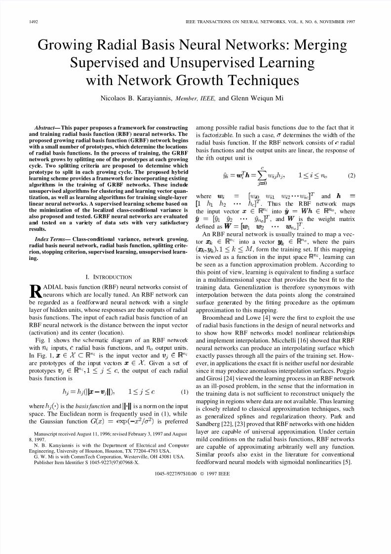
Fig. 1 shows the schematic diagram of an RBF network

with inputs, radial basis functions, and output units.

In Fig. 1, is the input vector and

are prototypes of the input vectors . Given a set of

prototypes , the output of each radial

basis function is

(1)

where is the basis function and is a norm on the input

space. The Euclidean norm is frequently used in (1), while

the Gaussian function is preferred

Manuscript received August 11, 1996; revised February 3, 1997 and August8, 1997.

N. B. Karayiannis is with the Department of Electrical and ComputerEngineering, University of Houston, Houston, TX 77204-4793 USA.

G. W. Mi is with CommTech Corporation, Westerville, OH 43081 USA.Publisher Item Identifier S 1045-9227(97)07968-X.

among possible radial basis functions due to the fact that it

is factorizable. In such a case, determines the width of the

radial basis function. If the RBF network consists of radial

basis functions and the output units are linear, the response of

the th output unit is

(2)

where and. Thus the RBF network maps

the input vector into , where

, and is the weight matrix

defined as .

An RBF neural network is usually trained to map a vec-

tor into a vector , where the pairs

, form the training set. If this mapping

is viewed as a function in the input space , learning can

be seen as a function approximation problem. According to

this point of view, learning is equivalent to finding a surface

in a multidimensional space that provides the best fit to the

training data. Generalization is therefore synonymous with

interpolation between the data points along the constrained

surface generated by the fitting procedure as the optimum

approximation to this mapping.

Broomhead and Lowe [4] were the first to exploit the use

of radial basis functions in the design of neural networks and

to show how RBF networks model nonlinear relationships

and implement interpolation. Micchelli [16] showed that RBF

neural networks can produce an interpolating surface which

exactly passes through all the pairs of the training set. How-

ever, in applications the exact fit is neither useful nor desirable

since it may produce anomalous interpolation surfaces. Poggio

and Girosi [24] viewed the learning process in an RBF network

as an ill-posed problem, in the sense that the information inthe training data is not sufficient to reconstruct uniquely the

mapping in regions where data are not available. Thus learningis closely related to classical approximation techniques, such

as generalized splines and regularization theory. Park and

Sandberg [22], [23] proved that RBF networks with one hidden

layer are capable of universal approximation. Under certain

mild conditions on the radial basis functions, RBF networks

are capable of approximating arbitrarily well any function.

Similar proofs also exist in the literature for conventional

feedforward neural models with sigmoidal nonlinearities [5].

1045–9227/97$10.00 © 1997 IEEE



KARAYIANNIS AND MI: GROWING RADIAL BASIS NEURAL NETWORKS 1493

Fig. 1. An RBF neural network.

The performance of an RBF network depends on the number

and positions of the radial basis functions, their shape, and the

method used for determining the associative weight matrix .

The existing learning strategies for RBF neural networks can

be classified as follows: 1) RBF networks with a fixed number

of radial basis function centers selected randomly from the

training data [4]; 2) RBF networks employing unsupervisedprocedures for selecting a fixed number of radial basis function

centers [18]; and 3) RBF networks employing supervised

procedures for selecting a fixed number of radial basis function

centers [11], [24].

Although some of the RBF neural networks mentioned

above are reported to be computationally efficient compared

with feedforward neural networks, they have the following

important drawback: the number of radial basis functions is

determined a priori. This leads to similar problems as the de-

termination of the number of hidden units for multilayer neural

networks [6], [9], [10], [15]. Several researchers attempted

to overcome this problem by determining the number and

locations of the radial basis function centers using constructiveand pruning methods.

Fritzke [7] attempted to solve this problem by the grow-

ing cell structure (GCS), a constructive method that allows

RBF neural networks to grow by inserting new prototypes

into positions in the feature space where the mapping needs

more details. Whitehead and Choate [26] proposed a similar

approach which evolves space-filling curves to distribute radial

basis functions over the input space. Berthold and Diamond [2]

introduced the dynamic decay adjustment (DDA) algorithm,

which works along with a constructive method to adjust the

decay factor (width) of each radial basis function. Musavi et

al. [19] eliminated the redundant prototypes by merging two

prototypes at each adaptation cycle.

This paper presents an alternative approach for constructing

and training growing radial basis function (GRBF) neural

networks. Section II proposes a hybrid scheme for constructing

and training GRBF neural networks. Section III presents a

variety of unsupervised and supervised algorithms that canbe used to determine the locations and widths of Gaussian

radial basis functions. Section IV presents learning schemes

for updating the synaptic weights of the upper associative

network based on recursive least-squares and gradient descent.

Section V presents criteria for splitting the prototypes of

GRBF neural networks during training and a stopping criterion

that can be used to terminate the learning process. Section VI

evaluates the performance of a variety of GRBF networks and

also compares their performance with that of conventional

RBF and feedforward neural networks. Section VII contains

concluding remarks.

II. A HYBRID LEARNING SCHEME

Each feature vector presented to an RBF network is mapped

into a vector of higher dimension formed by the responses of

the radial basis functions. Under certain conditions, such a

nonlinear mapping can transform a problem that is linearly

nonseparable in the feature space into a linearly separable

problem in a space of higher dimension. This transformation

depends on the number of radial basis functions, their widths,

and their locations in the feature space. The locations of

the radial basis functions are determined by the prototypes

representing the feature vectors. Because of the role of the




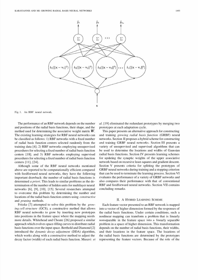
Fig. 2. The proposed construction and learning scheme for GRBF neural networks.

prototypes in the formation of the inputs of the upper network,

the partition of the input space produced by the existing

set of prototypes is of critical importance in RBF network

training. More specifically, the ability of an RBF network to

implement the desired mapping and the performance of the

trained network are both influenced by the resolution of thepartition induced upon the feature space by the prototypes. The

resolution of the partition is mainly determined by the a priori

selection of the number of prototypes. A rough partition could

make the training of the RBF network impossible. On the other

hand, a very fine partition of the feature space could force the

network to memorize the examples and, thus, compromise its

generalization ability.

The proposed approach allows GRBF networks to grow dur-

ing training by gradually increasing the number of prototypes

that represent the feature vectors in the training set and play the

role of the centers of the radial basis functions. The learning

process is roughly illustrated in Fig. 2. Learning begins by

determining the best two-partition of the feature space. Thiscan be accomplished by employing an unsupervised or a

supervised scheme. The two prototypes resulting in this phase

define a nontrivial partition of the lowest possible resolution. A

supervised learning scheme is subsequently employed to train

the upper associative network to give the desired responses

when presented with the outputs of the radial basis functions

generated by the available prototypes. If the upper associative

network is unable to learn the desired mapping, then a finer

partition of the feature space is created by splitting one of

the existing prototypes as indicated by a splitting criterion.

A partition of the feature space of higher resolution is sub-

sequently formed by using the existing set of prototypes as

the initial estimate. The prototypes corresponding to the new

partition are used to train the upper associative network. This

process is repeated until learning is terminated according to

a stopping criterion. The stopping criterion is based on the

success of the network to implement the desired input–outputmapping or the performance of the GRBF network. Splitting

and stopping criteria are working together to improve the

generalization ability of GRBF networks by preventing the

unnecessary splitting of the prototypes.

The proposed learning scheme for GRBF networks can be

summarized as follows:

1) Set . Initialize the prototypes .

2) Update the prototypes .

3) Update the widths of the radial basis functions.

4) Initialize the weights of the upper network.

5) Update the weights of the upper network.

6) If a stopping criterion is satisfied; then stop; else:7) Split one of the existing prototypes as indicated by a

splitting criterion.

8) Set and go to Step 2).

A GRBF network is constructed and trained in a sequence

of growing cycles. In the above learning scheme, a complete

growing cycle is described by Steps 2)–8). If a GRBF network

contains radial basis functions, it has gone through

growing cycles. The proposed construction/learning strategy is

compatible with any supervised or unsupervised technique that

can be used to map the feature vectors to the prototypes. It is

also compatible with a variety of supervised learning schemes












represented by are distributed over various classes. Each

prototype is also assigned an additional counter , defined

as . This counter gives

the maximum number of input vectors represented by the

prototype that belongs to a certain class. The least pure

prototype is selected for splitting according to

(28)

The purity splitting criterion is described in detail by the

following:

Set

For all

Determine such that

If is assigned to the th class

then

Determine

If

then split the th prototype.

B. Stopping Criterion

If the training set contains no overlapping data, then a

GRBF network can be trained until the error evaluated on the

training set becomes sufficiently small. In pattern classification

problems, for example, a GRBF can be trained until the

number of classification errors reduces to zero. In most pattern

classification applications, however, some training examples

from one class appear in a region of the feature space that

is mostly occupied by examples from another class. By in-

creasing the number of prototypes, each prototype would

represent very few training examples. This makes it possiblefor the network to map correctly onto its output training

examples in overlapping regions. However, such a strategy

would have a negative impact on the ability of the trained

network to generalize. This phenomenon is often referred to

in the literature as overtraining.

In order to avoid overtraining, the stopping criterion used

in this approach employs a testing or cross-validation set

in addition to the training set [8]. Both training and testing

sets are formed from the same data set. The errors on both

training and testing sets are recorded after each growing cycle.

Both these errors reduce at the early stages of learning. At a

certain point in the training process, the error on the testing

set begins increasing even though the error on the trainingset reduces. This is an indication of overtraining and can

be used to terminate the training process. In practice, the

point in time where overtraining begins is not clear because

of the fluctuation of both errors and the dependency on the

objective function. The following strategy is used in practice

to terminate training: Both errors are recorded after each

growing cycle. The network keeps growing even if there is a

temporary increase in the error evaluated on the testing set. The

status of the network (i.e., the weights of the upper network,

the prototypes, and the widths of the Gaussian functions) is

recorded if the error on the testing set decreases after a growing

cycle. If the error on the testing set does not decrease after

a sufficient number of growing cycles, then the training is

terminated while the network that resulted in the smallest error

on the testing set is the final product of the learning process.

VI. EXPERIMENTAL RESULTS

A. Two-Dimensional Vowel Data

In this set of experiments the performance of GRBF neural

networks was evaluated using a set of two-dimensional (2-D)

vowel data formed by computing the first two formants F1

and F2 from samples of ten vowels spoken by 67 speakers

[17], [20]. This data set has been extensively used to compare

different pattern classification approaches because there is

significant overlapping between the vectors corresponding to

different vowels in the F1-F2 plane [17], [20]. The available

671 feature vectors were divided into a training set, containing

338 vectors, and a testing set, containing 333 vectors.

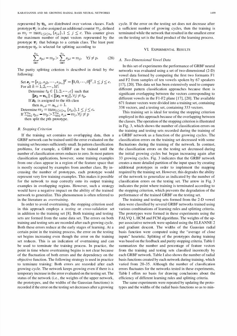
This training set is ideal for testing the stopping criterion

employed in this approach because of the overlapping betweenthe classes. The operation of the stopping criterion is illustrated

in Fig. 3, which shows the number of classification errors on

the training and testing sets recorded during the training of

a GRBF network as a function of the growing cycles. The

classification errors on the training set decreased with some

fluctuations during the training of the network. In contrast,

the classification errors on the testing set decreased during

the initial growing cycles but began increasing again after

33 growing cycles. Fig. 3 indicates that the GRBF network

creates a more detailed partition of the input space by creating

additional prototypes in order to implement the mapping

required by the training set. However, this degrades the ability

of the network to generalize as indicated by the number of classification errors on the testing set. The arrow in Fig. 3

indicates the point where training is terminated according to

the stopping criterion, which prevents the degradation of the

performance of the trained GRBF on the testing set.

The training and testing sets formed from the 2-D vowel

data were classified by several GRBF networks trained using

various combinations of learning rules and splitting criteria.

The prototypes were formed in these experiments using the

FALVQ 1, HCM and FCM algorithms. The weights of the up-

per associative network were updated using the ELEANNE 2

and gradient descent. The widths of the Gaussian radial

basis function were computed using the “average of close

inputs” heuristic. Splitting of the prototypes during trainingwas based on the feedback and purity stopping criteria. Table I

summarizes the number and percentage of feature vectors

from the training and testing sets classified incorrectly by

each GRBF network. Table I also shows the number of radial

basis functions created by each network during training, which

varied from 20–35. Although the number of classification

errors fluctuates for the networks tested in these experiments,

Table I offers no basis for drawing conclusions about the

efficiency of different learning rules and splitting criteria.

The same experiments were repeated by updating the proto-

types and the widths of the radial basis functions so as to min-




Fig. 3. Number of feature vectors from the training and testing sets formed from the 2-D vowel data classified incorrectly by the GRBF network as a functionof the number of growing cycles. The arrow indicates termination of training according to the stopping criterion employed.

TABLE ITHE PERFORMANCE OF VARIOUS GRBF NETWORKS EVALUATED ON THE 2-D VOWEL DATA SET: NUMBER /PERCENTAGE OF INCORRECTLY

CLASSIFIED FEATURE VECTORS FROM THE TRAINING SET( E

t r a i n

= % E

t r a i n

)

AND THE TESTING SET( E

t e s t

= % E

t e s t

)

AND THE

FINAL NUMBERc

OF RADIAL BASIS FUNCTIONS. PARAMETER SETTING: N = 3 0 ;

0

= 0 : 0 0 1

FOR FALVQ 1; = 0 : 0 0 0 1

FOR HCM; = 0 : 0 0 0 1 ; m = 1 : 1 FOR FCM; = 0 : 5 ; = 0 : 0 0 1 FOR ELEANNE 2; = 0 : 0 0 1 ; = 0 : 0 0 1 FOR GRADIENT DESCENT

imize the localized class-conditional variance. The ELEANNE

2 and gradient descent were used to update the weights of the

upper associative network while splitting of the prototypes was

based on the feedback and purity splitting criteria. The results

of these experiments are summarized in Table II. Comparison

of the average number of classification errors summarized in

Tables I and II indicates that updating the prototypes and the

widths of the radial basis functions by minimizing the localized

class-conditional variance improved the performance of the

trained GRBF networks on both training and testing sets. On

the average, these learning rules resulted in trained GRBF

networks with fewer radial basis functions.




TABLE IITHE PERFORMANCE OF VARIOUS GRBF NETWORKS EVALUATED ON THE

2-D VOWEL DATA SET: NUMBER /PERCENTAGE OF FEATURE VECTORS

FROM THE TRAINING SET ( E

t r a i n

= % E

t r a i n

) AND THE TESTING SET

( E

t e s t

= % E

t e s t

) CLASSIFIED INCORRECTLY AND THE FINAL NUMBER

c OF RADIAL BASIS FUNCTIONS. THE PROTOTYPES AND WIDTHS OF

THE RADIAL BASIS FUNCTIONS WERE UPDATED BY MINIMIZING THE

LOCALIZED CLASS-CONDITIONAL VARIANCE. PARAMETER SETTING: = 0 : 5 ; = 0 : 0 0 1 FOR ELEANNE 2; = 0 : 0 0 1 ; = 0 : 0 0 1 FOR GRADIENT

DESCENT; = 0 : 0 0 1 FOR CLASS-CONDITIONAL VARIANCE MINIMIZATION

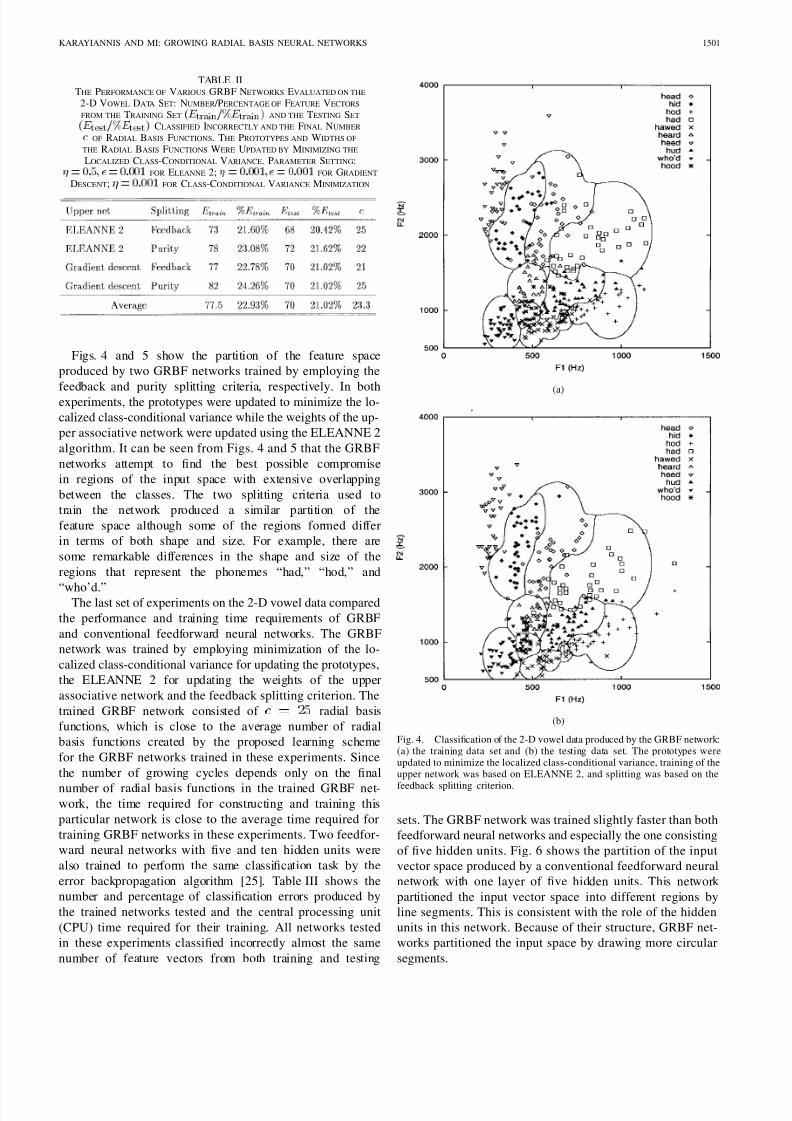
Figs. 4 and 5 show the partition of the feature space

produced by two GRBF networks trained by employing the

feedback and purity splitting criteria, respectively. In bothexperiments, the prototypes were updated to minimize the lo-

calized class-conditional variance while the weights of the up-

per associative network were updated using the ELEANNE 2

algorithm. It can be seen from Figs. 4 and 5 that the GRBF

networks attempt to find the best possible compromise

in regions of the input space with extensive overlapping

between the classes. The two splitting criteria used to

train the network produced a similar partition of the

feature space although some of the regions formed differ

in terms of both shape and size. For example, there are

some remarkable differences in the shape and size of the

regions that represent the phonemes “had,” “hod,” and

“who’d.”The last set of experiments on the 2-D vowel data compared

the performance and training time requirements of GRBF

and conventional feedforward neural networks. The GRBF

network was trained by employing minimization of the lo-

calized class-conditional variance for updating the prototypes,

the ELEANNE 2 for updating the weights of the upper

associative network and the feedback splitting criterion. The

trained GRBF network consisted of radial basis

functions, which is close to the average number of radial

basis functions created by the proposed learning scheme

for the GRBF networks trained in these experiments. Since

the number of growing cycles depends only on the final

number of radial basis functions in the trained GRBF net-work, the time required for constructing and training this

particular network is close to the average time required for

training GRBF networks in these experiments. Two feedfor-

ward neural networks with five and ten hidden units were

also trained to perform the same classification task by the

error backpropagation algorithm [25]. Table III shows the

number and percentage of classification errors produced by

the trained networks tested and the central processing unit

(CPU) time required for their training. All networks tested

in these experiments classified incorrectly almost the same

number of feature vectors from both training and testing

(a)

(b)

Fig. 4. Classification of the 2-D vowel data produced by the GRBF network:(a) the training data set and (b) the testing data set. The prototypes wereupdated to minimize the localized class-conditional variance, training of theupper network was based on ELEANNE 2, and splitting was based on the

feedback splitting criterion.

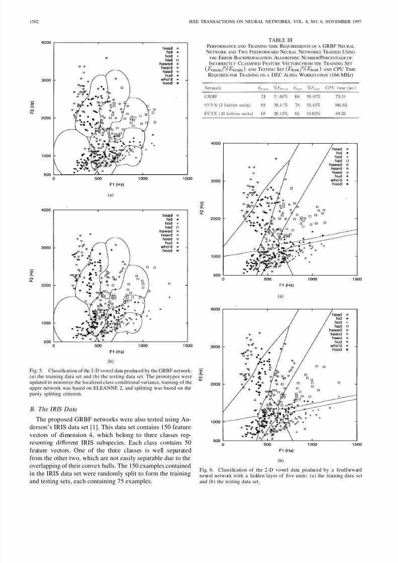
sets. The GRBF network was trained slightly faster than both

feedforward neural networks and especially the one consisting

of five hidden units. Fig. 6 shows the partition of the input

vector space produced by a conventional feedforward neural

network with one layer of five hidden units. This network

partitioned the input vector space into different regions byline segments. This is consistent with the role of the hidden

units in this network. Because of their structure, GRBF net-

works partitioned the input space by drawing more circular

segments.




(a)

(b)

Fig. 5. Classification of the 2-D vowel data produced by the GRBF network:(a) the training data set and (b) the testing data set. The prototypes wereupdated to minimize the localized class-conditional variance, training of theupper network was based on ELEANNE 2, and splitting was based on the

purity splitting criterion.

B. The IRIS Data

The proposed GRBF networks were also tested using An-

derson’s IRIS data set [1]. This data set contains 150 feature

vectors of dimension 4, which belong to three classes rep-

resenting different IRIS subspecies. Each class contains 50

feature vectors. One of the three classes is well separated

from the other two, which are not easily separable due to the

overlapping of their convex hulls. The 150 examples contained

in the IRIS data set were randomly split to form the training

and testing sets, each containing 75 examples.

TABLE IIIPERFORMANCE AND TRAINING TIME REQUIREMENTS OF A GRBF NEURAL

NETWORK AND TWO FEEDFORWARD NEURAL NETWORKS TRAINED USING

THE ERROR BACKPROPAGATION ALGORITHM: NUMBER /PERCENTAGE OF

INCORRECTLY CLASSIFIED FEATURE VECTORS FROM THE TRAINING SET

( E

t r a i n

= % E

t r a i n

) AND TESTING SET ( E

t e s t

= % E

t e s t

) AND CPU TIME

REQUIRED FOR TRAINING ON A DEC ALPHA WORKSTATION (166 MHz)

(a)

(b)

Fig. 6. Classification of the 2-D vowel data produced by a feedforwardneural network with a hidden layer of five units: (a) the training data setand (b) the testing data set.




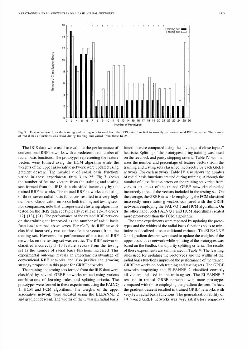
Fig. 7. Feature vectors from the training and testing sets formed from the IRIS data classified incorrectly by conventional RBF networks. The numberof radial basis functions was fixed during training and varied from three to 25.

The IRIS data were used to evaluate the performance of

conventional RBF networks with a predetermined number of

radial basis functions. The prototypes representing the feature

vectors were formed using the HCM algorithm while the

weights of the upper associative network were updated using

gradient descent. The number of radial basis functions

varied in these experiments from 3 to 25. Fig. 7 shows

the number of feature vectors from the training and testing

sets formed from the IRIS data classified incorrectly by the

trained RBF networks. The trained RBF networks consisting

of three–seven radial basis functions resulted in a very high

number of classification errors on both training and testing sets.

For comparison, note that unsupervised clustering algorithms

tested on the IRIS data set typically result in 12–17 errors

[12], [13], [21]. The performance of the trained RBF network

on the training set improved as the number of radial basis

functions increased above seven. For the RBF network

classified incorrectly two or three feature vectors from the

training set. However, the performance of the trained RBF

networks on the testing set was erratic. The RBF networks

classified incorrectly 3–13 feature vectors from the testingset as the number of radial basis functions increased. This

experimental outcome reveals an important disadvantage of

conventional RBF networks and also justifies the growing

strategy proposed in this paper for GRBF networks.

The training and testing sets formed from the IRIS data were

classified by several GRBF networks trained using various

combinations of learning rules and splitting criteria. The

prototypes were formed in these experiments using the FALVQ

1, HCM and FCM algorithms. The weights of the upper

associative network were updated using the ELEANNE 2

and gradient descent. The widths of the Gaussian radial basis

function were computed using the “average of close inputs”

heuristic. Splitting of the prototypes during training was based

on the feedback and purity stopping criteria. Table IV summa-

rizes the number and percentage of feature vectors from the

training and testing sets classified incorrectly by each GRBF

network. For each network, Table IV also shows the number

of radial basis functions created during training. Although the

number of classification errors on the training set varied fromzero to six, most of the trained GRBF networks classified

incorrectly three of the vectors included in the testing set. On

the average, the GRBF networks employing the FCM classified

incorrectly more training vectors compared with the GRBF

networks employing the FALVQ 1 and HCM algorithms. On

the other hand, both FALVQ 1 and HCM algorithms created

more prototypes than the FCM algorithm.

The same experiments were repeated by updating the proto-

types and the widths of the radial basis functions so as to min-

imize the localized class-conditional variance. The ELEANNE

2 and gradient descent were used to update the weights of the

upper associative network while splitting of the prototypes was

based on the feedback and purity splitting criteria. The resultsof these experiments are summarized in Table V. The learning

rules used for updating the prototypes and the widths of the

radial basis functions improved the performance of the trained

GRBF networks on both training and testing sets. The GRBF

networks employing the ELEANNE 2 classified correctly

all vectors included in the training set. The ELEANNE 2

resulted in trained GRBF networks with more prototypes

compared with those employing the gradient descent. In fact,

the gradient descent resulted in trained GRBF networks with

very few radial basis functions. The generalization ability of

all trained GRBF networks was very satisfactory regardless




TABLE IVTHE PERFORMANCE OF VARIOUS GRBF NETWORKS EVALUATED ON THE IRIS DATA SET: NUMBER /PERCENTAGE OF INCORRECTLY CLASSIFIED

FEATURE VECTORS FROM THE TRAINING SET ( E

t r a i n

= % E

t r a i n

) AND THE TESTING SET ( E

t e s t

= % E

t e s t

) AND THE FINAL

NUMBER c OF RADIAL BASIS FUNCTIONS. PARAMETER SETTING: N = 3 0 ;

0

= 0 : 0 1 FOR FALVQ 1; = 0 : 0 0 0 1 FOR HCM; = 0 : 0 0 0 1 ; m = 1 : 1 FOR FCM; = 1 : 0 ; = 0 : 0 0 0 5 FOR ELEANNE 2; = 0 : 0 1 ; = 0 : 0 0 0 5 FOR GRADIENT DESCENT

TABLE VTHE PERFORMANCE OF VARIOUS GRBF NETWORKS EVALUATED ON THE IRIS

DATA SET: NUMBER /PERCENTAGE OF FEATURE VECTORS FROM THE TRAINING

SET ( E

t r a i n

= % E

t r a i n

) AND THE TESTING SET ( E

t e s t

= % E

t e s t

)

CLASSIFIED INCORRECTLY AND THE FINAL NUMBERc

OF RADIAL BASIS

FUNCTIONS. THE PROTOTYPES AND WIDTHS OF THE RADIAL BASIS

FUNCTIONS WERE UPDATED BY MINIMIZING THE LOCALIZED

CLASS-CONDITIONAL VARIANCE. PARAMETER SETTING: = 1 : 0 ; = 0 : 0 0 0 5

FOR ELEANNE 2; = 0 : 0 1 ; = 0 : 0 0 0 5 FOR GRADIENT DESCENT; = 0 : 0 0 5 FOR CLASS-CONDITIONAL VARIANCE MINIMIZATION

of the learning scheme employed for updating the weightsof the upper associative network. With only one exception,

the GRBF networks trained in these experiments classified

incorrectly only one vector from the testing set.

VII. CONCLUSIONS

This paper presented the development, testing, and evalua-

tion of a framework for constructing and training growing RBF

neural networks. The hybrid learning scheme proposed in this

paper allows the participation of the training set in the creation

of the prototypes, even if the prototypes are created using

an unsupervised algorithm. This is accomplished through the

proposed splitting criteria, which relate directly to the training

set and create prototypes in certain locations of the input space

which are crucial for the implementation of the input–output

mapping. This strategy allows the representation of the input

space of different resolution levels by creating few prototypes

to represent smooth regions in the input space and utilizing

the available resources where they are actually necessary.The stopping criterion employed in this paper prevents the

creation of degenerate prototypes that could compromise the

generalization ability of trained GRBF networks by stopping

their growth as indicated by their performance on a testing

set. The proposed hybrid scheme is compatible with a variety

of unsupervised clustering and LVQ algorithms that can be

used to determine the locations and widths of the radial

basis functions. This paper also proposed a new supervised

scheme for updating the locations and widths of the radial

basis functions during learning. This scheme is based on

the minimization of a localized class-conditional variance

measure, which is computed from the outputs of the radialbasis functions and relates to the structure of the feature

space.

A variety of learning algorithms were employed in this

paper for constructing and training GRBF neural networks.

The weights of the upper associative network were updated

in the experiments using the ELEANNE 2, a recursive least-

squares algorithm, and gradient descent. The prototypes were

updated by an enhanced version of the -means algorithm,

the fuzzy -means algorithm, and the FALVQ 1 algorithm.

The localized class-conditional variance criterion was also

used in the experiments to update the prototypes as well as




the widths of the radial basis functions. The performance

of the trained GRBF networks was compared with that of

conventional RBF and feedforward neural networks. The ex-

periments revealed a significant limitation of RBF neural

networks with a fixed number of hidden units: Increasing the

number of radial basis functions did not significantly improve

their performance. In fact, trained GRBF neural networks

performed better than conventional RBF networks containing

a larger number of radial basis functions. If the prototypes

are created by an unsupervised process, the inferior perfor-

mance of conventional RBF networks can be attributed to thefollowing reasons: 1) The training set does not participate in

the creation of the prototypes which is based on the criterion

used for developing the clustering and LVQ algorithm. 2)

The unsupervised algorithm can waste the resources of the

network, namely the radial basis functions, by creating proto-

types in insignificant regions while ignoring regions which

are important for implementing the input–output mapping.

The experiments indicated that the performance of trained

GRBF networks is mostly affected by the algorithm used for

updating the prototypes after splitting. The GRBF networksemploying minimization of the localized class-conditional

variance achieved the most robust performance in pattern

classification tasks among those tested in the experiments.

What distinguishes this learning scheme from those employing

unsupervised algorithms to update the prototypes is that the

input vectors are treated as labeled feature vectors during

training. Thus, the training set has a direct impact on the

formation of the prototypes in addition to its role in the

splitting of the prototypes.

APPENDIX

Updating the Locations of Radial Basis Functions

The gradient of with respect to the prototype thatdetermines the location of the th radial basis function is

(A1)

From the definition of in (8)

(A2)

Since

(A3)

where

(A4)

The definition of in (11) gives

(A5)

where

(A6)

The gradient of with respect to can be obtained from

(A1) after combining (A2) with (A3) and (A5) as

(A7)

Updating the Widths of Radial Basis Functions

The gradient of with respect to the width of the th radial

basis function is

(A8)

From the definition of in (8)

(A9)

Since

(A10)

where

(A11)

The definition of in (11) gives

(A12)

where

(A13)

The gradient of with respect to can be obtained from

(A8) after combining (A9) with (A10) and (A12) as

(A14)




REFERENCES

[1] E. Anderson, “The IRISes of the Gaspe peninsula,” Bull. Amer. IRISSoc., vol. 59, pp. 2–5, 1939.

[2] M. R. Berthold and J. Diamond, “Boosting the performance of RBFnetworks with dynamic decay adjustment,” in Advances in Neural

Inform. Processing Syst. 3, R. P. Lippmann et al., Eds. San Mateo,CA: Morgan Kaufmann, 1991.

[3] J. C. Bezdek, Pattern Recognition with Fuzzy Objective Function Algo-rithms. New York: Plenum, 1981.

[4] D. S. Broomhead and D. Lowe, “Multivariable functional interpolationand adaptive networks,” Complex Syst., vol. 2, pp. 321–355, 1988.[5] G. Cybenko, “Approximation by superpositions of a sigmoidal func-

tion,” Math. Contr., Signals, Syst., vol. 2, pp. 303–314, 1989.[6] S. E. Fahlman and C. Lebiere, “The cascade-correlation learning ar-

chitecture,” in Advances in Neural Information Processing Systems 2,D. S. Touretzky, Ed. San Mateo, CA: Morgan Kaufmann, 1990, pp.524–532.

[7] B. Fritzke, “Growing cell structures—A self-organizing network forunsupervised and supervised learning,” Int. Computer Sci. Inst., Univ.California at Berkeley, Tech. Rep. TR–93–026, May 1993.

[8] R. Hecht–Nielsen, Neurocomputing. Reading, MA: Addison-Wesley,1990.

[9] J.–N. Hwang, “The cascade-correlation learning: A projection pur-suit learning perspective,” IEEE Trans. Neural Networks, vol. 7, pp.278–289, 1996.

[10] N. B. Karayiannis, “ALADIN: Algorithms for learning and architecturedetermination,” IEEE Trans. Circuits Syst., vol. 41, pp. 752–759, 1994.

[11] , “Gradient descent learning of radial basis neural networks,” inProc. 1997 Int. Conf. Neural Networks (ICNN ’97), Houston, TX, June9–12, 1997, pp. 1815–1820.

[12] , “A methodology for constructing fuzzy algorithms for learningvector quantization,” IEEE Trans. Neural Networks, vol. 8, pp. 505–518,1997.

[13] N. B. Karayiannis and P.-I Pai, “Fuzzy algorithms for learning vectorquantization,” IEEE Trans. Neural Networks, vol. 7, pp. 1196–1211,1996.

[14] N. B. Karayiannis and A. N. Venetsanopoulos, “Efficient learningalgorithms for neural networks (ELEANNE),” IEEE Trans. Syst., Man,Cybern., vol. 23, pp. 1372–1383, 1993.

[15] , Artificial Neural Networks: Learning Algorithms, Performance Evaluation, and Applications. Boston, MA: Kluwer, 1993.

[16] C. A. Micchelli, “Interpolation of scattered data: Distance matrices andconditionally positive definite functions,” Constructive Approximation,vol. 2, pp. 11–22, 1986.

[17] R. P. Lippmann, “Pattern classification using neural networks,” IEEE Commun. Mag., vol. 27, pp. 47–54, 1989.

[18] J. E. Moody and C. J. Darken, “Fast learning in networks of locally-tuned processing units,” Neural Computa., vol. 1, pp. 281–294, 1989.

[19] M. T. Musavi, W. Ahmed, K. H. Chan, K. B. Faris, and D. M. Hummels,“On the training of radial basis function classifiers,” Neural Networks,vol. 5, pp. 595–603, 1992.

[20] K. Ng and R. P. Lippmann, “Practical characteristics of neural network and conventional pattern classifiers,” in Advances in Neural Inform.Processing Syst. 3, R. P. Lippmann et al., Eds. San Mateo, CA: MorganKaufmann, 1991, pp. 970–976.

[21] N. R. Pal, J. C. Bezdek, and E. C.-K. Tsao, “Generalized clustering

networks and Kohonen’s self-organizing scheme,” IEEE Trans. Neural Networks, vol. 4, pp. 549–557, 1993.[22] J. Park and I. W. Sandberg, “Universal approximation using radial basis

function networks,” Neural Computa., vol. 3, pp. 246–257, 1991.[23] , “Approximation and radial basis function networks,” Neural

Computa., vol. 5, pp. 305–316, 1993.[24] T. Poggio and F. Girosi, “Regularization algorithms for learning that

are equivalent to multilayer networks,” Science, vol. 247, pp. 978–982,1990.

[25] D. E. Rumelhart, G. E. Hinton, and R. J. Williams, “Learning internalrepresentations by error propagation,” in Parallel Distributed Process-ing, D. E. Rumelhart and J. L. McClelland, Eds., vol. I. Cambridge,MA: MIT Press, 1986, pp. 318–362.

[26] B. A. Whitehead and T. D. Choate, “Evolving space-filling curves todistribute radial basis functions over an input space,” IEEE Trans. Neural

Networks, vol. 5, pp. 15–23, 1994.

Nicolaos B. Karayiannis (S’85–M’91), for a photograph and biography, seethe May 1997 issue of this TRANSACTIONS, p. 518.

Glenn Weiqun Mi was born in Shanghai, China, in1968. He received the B.S. degree from the Depart-ment of Electronic Engineering, Fudan University,Shanghai, China, in 1990, and the M.S. degreefrom the Department of Electrical and ComputerEngineering, University of Houston, in 1996.

He is currently a software engineer in CommTechCorporation, Columbus, OH. His research interestsinclude radial basis neural networks, supervised and

unsupervised learning, and vector quantization.

Documents

(Đề tài cô gửi) Karayiannis_tnn_8(6)_97