De ning the climatic signal in stream salinity trends

Defining the climatic signal in stream salinity trends

using the Interdecadal Pacific Oscillation and its rate of

change

V. H. Mcneil, M. E. Cox

To cite this version:

V. H. Mcneil, M. E. Cox. Defining the climatic signal in stream salinity trends using theInterdecadal Pacific Oscillation and its rate of change. Hydrology and Earth System SciencesDiscussions, European Geosciences Union, 2007, 11 (4), pp.1295-1307. <hal-00305074>

HAL Id: hal-00305074

https://hal.archives-ouvertes.fr/hal-00305074

Submitted on 3 May 2007

HAL is a multi-disciplinary open accessarchive for the deposit and dissemination of sci-entific research documents, whether they are pub-lished or not. The documents may come fromteaching and research institutions in France orabroad, or from public or private research centers.

L’archive ouverte pluridisciplinaire HAL, estdestinee au depot et a la diffusion de documentsscientifiques de niveau recherche, publies ou non,emanant des etablissements d’enseignement et derecherche francais ou etrangers, des laboratoirespublics ou prives.

brought to you by COREView metadata, citation and similar papers at core.ac.uk

provided by HAL-INSU

https://core.ac.uk/display/52752088?utm_source=pdf&utm_medium=banner&utm_campaign=pdf-decoration-v1

https://hal.archives-ouvertes.fr

https://hal.archives-ouvertes.fr/hal-00305074

Hydrol. Earth Syst. Sci., 11, 1295–1307, 2007www.hydrol-earth-syst-sci.net/11/1295/2007/© Author(s) 2007. This work is licensedunder a Creative Commons License.

Hydrology andEarth System

Sciences

Defining the climatic signal in stream salinity trends using theInterdecadal Pacific Oscillation and its rate of change

V. H. McNeil1 and M. E. Cox2

1Resource Sciences and Knowledge, Department of Natural Resources and Water, Brisbane, Qld, Australia2School of Natural Resource Sciences, Queensland University of Technology, Brisbane, Qld, Australia

Received: 27 March 2006 – Published in Hydrol. Earth Syst. Sci. Discuss.: 20 September 2006Revised: 13 March 2007 – Accepted: 23 March 2007 – Published: 3 May 2007

Abstract. The impact of landuse on stream salinity iscurrently difficult to separate from the effect of climate,as the decadal scale climatic cycles in groundwater andstream hydrology have similar wavelengths to the landusepattern. These hydrological cycles determine the streamsalinity through accumulation or release of salt in the land-scape. Widespread patterns apparent in stream salinity arediscussed, and a link is demonstrated between stream salin-ity, groundwater levels and global climatic indicators. TheInterdecadal Pacific Oscillation (IPO) has previously beeninvestigated as a contributory climatic indicator for hydro-logical and related time series in the Southern Hemisphere.This study presents an approach which explores the rate ofchange in the IPO, in addition to its value, to define an indica-tor for the climate component of ambient shallow groundwa-ter levels and corresponding stream salinity. Composite timeseries of groundwater level and stream salinity are compiledusing an extensive but irregular database covering a wide ge-ographical area. These are modelled with respect to the IPOand its rate of change to derive control time series. A exam-ple is given of how a stream salinity trend changes when thedecadal climatic influence is removed.

1 Introduction

This work arose originally from the recognition of patternsin stream salinity on a regional basis. Variations or trendsin salinity represented by Electrical Conductivity (EC) canbe significant and have often been measured as a potentialindicator of landuse sustainability issues. These issues in-clude the incipient development of dryland salinity, impactsof land clearing, irrigation, drainage alterations, and urban-isation (for instance, Ruprecht and Schofield, 1991). EC

Correspondence to: V. H. McNeil([email protected])

monitoring is relatively low cost and convenient to automate.However, it can only be relied on to define long-term humanimpact if such impacts can be distinguished from variationsthat result from broad climate fluctuations.

A control site is needed which has the same climate char-acteristics but without the local landuse effect. However, par-ticularly for large catchments, comparable undisturbed sitesmay not be available. The likelihood of a consistent patternin the climate effect over a large area offers the possibility ofdeveloping a composite climate control by aggregating ECdata widely and using global climate indicators to verify thatthe broadscale pattern is, in fact, a climate signal.

Accordingly, the purpose of this study is to verify thatdecadal scale climatic trends are present in records ofQueensland stream salinity and its associated groundwaterhydrology by relating the records to global climatic indica-tors.

1.1 Recognition of broadscale decadal patterns in streamsalinity trends

The influence of climatic fluctuations on stream salinity wasrecognised in a previous study (QDPI, 1994) where ECtrends were calculated for around 500 stream gauging sta-tions throughout the state of Queensland covering a twentyyear period between 1970 and 1990, in a project to inves-tigate the impact of changes in landuse. It was expected atthe time that the climatic contribution would present as localrandom noise overlying longer-term trends representative oflocal landuse changes.

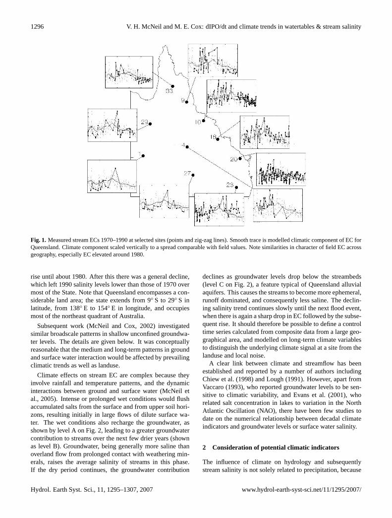
Instead of the expected generally flat EC trends with risesor crests in areas where rapid development had occurred, acomplex but consistent trend pattern was evident in manystreams, over a very diverse range of topography, geologyand landuse. Some examples from the 1994 study are shownon Fig. 1. It can be seen that many of the streams had rela-tively low ECs during the early 1970s, followed by a steady

Published by Copernicus GmbH on behalf of the European Geosciences Union.

1296 V. H. McNeil and M. E. Cox: dIPO/dt and climate trends in watertables & stream salinity

Fig. 1. Measured stream ECs 1970–1990 at selected sites (points and zig-zag lines). Smooth trace is modelled climatic component of EC forQueensland. Climate component scaled vertically to a spread comparable with field values. Note similarities in character of field EC acrossgeography, especially EC elevated around 1980.

rise until about 1980. After this there was a general decline,which left 1990 salinity levels lower than those of 1970 overmost of the State. Note that Queensland encompasses a con-siderable land area; the state extends from 9◦ S to 29◦ S inlatitude, from 138◦ E to 154◦ E in longitude, and occupiesmost of the northeast quadrant of Australia.

Subsequent work (McNeil and Cox, 2002) investigatedsimilar broadscale patterns in shallow unconfined groundwa-ter levels. The details are given below. It was conceptuallyreasonable that the medium and long-term patterns in groundand surface water interaction would be affected by prevailingclimatic trends as well as landuse.

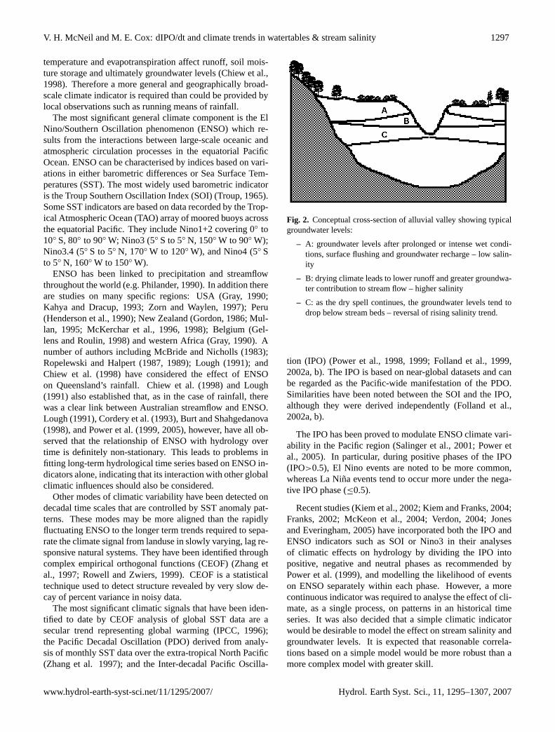
Climate effects on stream EC are complex because theyinvolve rainfall and temperature patterns, and the dynamicinteractions between ground and surface water (McNeil etal., 2005). Intense or prolonged wet conditions would flushaccumulated salts from the surface and from upper soil hori-zons, resulting initially in large flows of dilute surface wa-ter. The wet conditions also recharge the groundwater, asshown by level A on Fig. 2, leading to a greater groundwatercontribution to streams over the next few drier years (shownas level B). Groundwater, being generally more saline thanoverland flow from prolonged contact with weathering min-erals, raises the average salinity of streams in this phase.If the dry period continues, the groundwater contribution

declines as groundwater levels drop below the streambeds(level C on Fig. 2), a feature typical of Queensland alluvialaquifers. This causes the streams to become more ephemeral,runoff dominated, and consequently less saline. The declin-ing salinity trend continues slowly until the next flood event,when there is again a sharp drop in EC followed by the subse-quent rise. It should therefore be possible to define a controltime series calculated from composite data from a large geo-graphical area, and modelled on long-term climate variablesto distinguish the underlying climate signal at a site from thelanduse and local noise.

A clear link between climate and streamflow has beenestablished and reported by a number of authors includingChiew et al. (1998) and Lough (1991). However, apart fromVaccaro (1993), who reported groundwater levels to be sen-sitive to climatic variability, and Evans et al. (2001), whorelated salt concentration in lakes to variation in the NorthAtlantic Oscillation (NAO), there have been few studies todate on the numerical relationship between decadal climateindicators and groundwater levels or surface water salinity.

2 Consideration of potential climatic indicators

The influence of climate on hydrology and subsequentlystream salinity is not solely related to precipitation, because

Hydrol. Earth Syst. Sci., 11, 1295–1307, 2007 www.hydrol-earth-syst-sci.net/11/1295/2007/

V. H. McNeil and M. E. Cox: dIPO/dt and climate trends in watertables & stream salinity 1297

temperature and evapotranspiration affect runoff, soil mois-ture storage and ultimately groundwater levels (Chiew et al.,1998). Therefore a more general and geographically broad-scale climate indicator is required than could be provided bylocal observations such as running means of rainfall.

The most significant general climate component is the ElNino/Southern Oscillation phenomenon (ENSO) which re-sults from the interactions between large-scale oceanic andatmospheric circulation processes in the equatorial PacificOcean. ENSO can be characterised by indices based on vari-ations in either barometric differences or Sea Surface Tem-peratures (SST). The most widely used barometric indicatoris the Troup Southern Oscillation Index (SOI) (Troup, 1965).Some SST indicators are based on data recorded by the Trop-ical Atmospheric Ocean (TAO) array of moored buoys acrossthe equatorial Pacific. They include Nino1+2 covering 0◦ to10◦ S, 80◦ to 90◦ W; Nino3 (5◦ S to 5◦ N, 150◦ W to 90◦ W);Nino3.4 (5◦ S to 5◦ N, 170◦ W to 120◦ W), and Nino4 (5◦ Sto 5◦ N, 160◦ W to 150◦ W).

ENSO has been linked to precipitation and streamflowthroughout the world (e.g. Philander, 1990). In addition thereare studies on many specific regions: USA (Gray, 1990;Kahya and Dracup, 1993; Zorn and Waylen, 1997); Peru(Henderson et al., 1990); New Zealand (Gordon, 1986; Mul-lan, 1995; McKerchar et al., 1996, 1998); Belgium (Gel-lens and Roulin, 1998) and western Africa (Gray, 1990). Anumber of authors including McBride and Nicholls (1983);Ropelewski and Halpert (1987, 1989); Lough (1991); andChiew et al. (1998) have considered the effect of ENSOon Queensland’s rainfall. Chiew et al. (1998) and Lough(1991) also established that, as in the case of rainfall, therewas a clear link between Australian streamflow and ENSO.Lough (1991), Cordery et al. (1993), Burt and Shahgedanova(1998), and Power et al. (1999, 2005), however, have all ob-served that the relationship of ENSO with hydrology overtime is definitely non-stationary. This leads to problems infitting long-term hydrological time series based on ENSO in-dicators alone, indicating that its interaction with other globalclimatic influences should also be considered.

Other modes of climatic variability have been detected ondecadal time scales that are controlled by SST anomaly pat-terns. These modes may be more aligned than the rapidlyfluctuating ENSO to the longer term trends required to sepa-rate the climate signal from landuse in slowly varying, lag re-sponsive natural systems. They have been identified throughcomplex empirical orthogonal functions (CEOF) (Zhang etal., 1997; Rowell and Zwiers, 1999). CEOF is a statisticaltechnique used to detect structure revealed by very slow de-cay of percent variance in noisy data.

The most significant climatic signals that have been iden-tified to date by CEOF analysis of global SST data are asecular trend representing global warming (IPCC, 1996);the Pacific Decadal Oscillation (PDO) derived from analy-sis of monthly SST data over the extra-tropical North Pacific(Zhang et al. 1997); and the Inter-decadal Pacific Oscilla-

Fig. 2. Conceptual cross-section of alluvial valley showing typicalgroundwater levels:

– A: groundwater levels after prolonged or intense wet condi-tions, surface flushing and groundwater recharge – low salin-ity

– B: drying climate leads to lower runoff and greater groundwa-ter contribution to stream flow – higher salinity

– C: as the dry spell continues, the groundwater levels tend todrop below stream beds – reversal of rising salinity trend.

tion (IPO) (Power et al., 1998, 1999; Folland et al., 1999,2002a, b). The IPO is based on near-global datasets and canbe regarded as the Pacific-wide manifestation of the PDO.Similarities have been noted between the SOI and the IPO,although they were derived independently (Folland et al.,2002a, b).

The IPO has been proved to modulate ENSO climate vari-ability in the Pacific region (Salinger et al., 2001; Power etal., 2005). In particular, during positive phases of the IPO(IPO>0.5), El Nino events are noted to be more common,whereas La Nina events tend to occur more under the nega-tive IPO phase (≤0.5).

Recent studies (Kiem et al., 2002; Kiem and Franks, 2004;Franks, 2002; McKeon et al., 2004; Verdon, 2004; Jonesand Everingham, 2005) have incorporated both the IPO andENSO indicators such as SOI or Nino3 in their analysesof climatic effects on hydrology by dividing the IPO intopositive, negative and neutral phases as recommended byPower et al. (1999), and modelling the likelihood of eventson ENSO separately within each phase. However, a morecontinuous indicator was required to analyse the effect of cli-mate, as a single process, on patterns in an historical timeseries. It was also decided that a simple climatic indicatorwould be desirable to model the effect on stream salinity andgroundwater levels. It is expected that reasonable correla-tions based on a simple model would be more robust than amore complex model with greater skill.

www.hydrol-earth-syst-sci.net/11/1295/2007/ Hydrol. Earth Syst. Sci., 11, 1295–1307, 2007


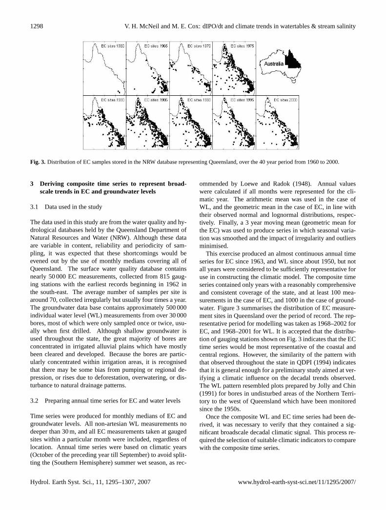
Fig. 3. Distribution of EC samples stored in the NRW database representing Queensland, over the 40 year period from 1960 to 2000.

3 Deriving composite time series to represent broad-scale trends in EC and groundwater levels

3.1 Data used in the study

The data used in this study are from the water quality and hy-drological databases held by the Queensland Department ofNatural Resources and Water (NRW). Although these dataare variable in content, reliability and periodicity of sam-pling, it was expected that these shortcomings would beevened out by the use of monthly medians covering all ofQueensland. The surface water quality database containsnearly 50 000 EC measurements, collected from 815 gaug-ing stations with the earliest records beginning in 1962 inthe south-east. The average number of samples per site isaround 70, collected irregularly but usually four times a year.The groundwater data base contains approximately 500 000individual water level (WL) measurements from over 30 000bores, most of which were only sampled once or twice, usu-ally when first drilled. Although shallow groundwater isused throughout the state, the great majority of bores areconcentrated in irrigated alluvial plains which have mostlybeen cleared and developed. Because the bores are partic-ularly concentrated within irrigation areas, it is recognisedthat there may be some bias from pumping or regional de-pression, or rises due to deforestation, overwatering, or dis-turbance to natural drainage patterns.

3.2 Preparing annual time series for EC and water levels

Time series were produced for monthly medians of EC andgroundwater levels. All non-artesian WL measurements nodeeper than 30 m, and all EC measurements taken at gaugedsites within a particular month were included, regardless oflocation. Annual time series were based on climatic years(October of the preceding year till September) to avoid split-ting the (Southern Hemisphere) summer wet season, as rec-

ommended by Loewe and Radok (1948). Annual valueswere calculated if all months were represented for the cli-matic year. The arithmetic mean was used in the case ofWL, and the geometric mean in the case of EC, in line withtheir observed normal and lognormal distributions, respec-tively. Finally, a 3 year moving mean (geometric mean forthe EC) was used to produce series in which seasonal varia-tion was smoothed and the impact of irregularity and outliersminimised.

This exercise produced an almost continuous annual timeseries for EC since 1963, and WL since about 1950, but notall years were considered to be sufficiently representative foruse in constructing the climatic model. The composite timeseries contained only years with a reasonably comprehensiveand consistent coverage of the state, and at least 100 mea-surements in the case of EC, and 1000 in the case of ground-water. Figure 3 summarises the distribution of EC measure-ment sites in Queensland over the period of record. The rep-resentative period for modelling was taken as 1968–2002 forEC, and 1968–2001 for WL. It is accepted that the distribu-tion of gauging stations shown on Fig. 3 indicates that the ECtime series would be most representative of the coastal andcentral regions. However, the similarity of the pattern withthat observed throughout the state in QDPI (1994) indicatesthat it is general enough for a preliminary study aimed at ver-ifying a climatic influence on the decadal trends observed.The WL pattern resembled plots prepared by Jolly and Chin(1991) for bores in undisturbed areas of the Northern Terri-tory to the west of Queensland which have been monitoredsince the 1950s.

Once the composite WL and EC time series had been de-rived, it was necessary to verify that they contained a sig-nificant broadscale decadal climatic signal. This process re-quired the selection of suitable climatic indicators to comparewith the composite time series.



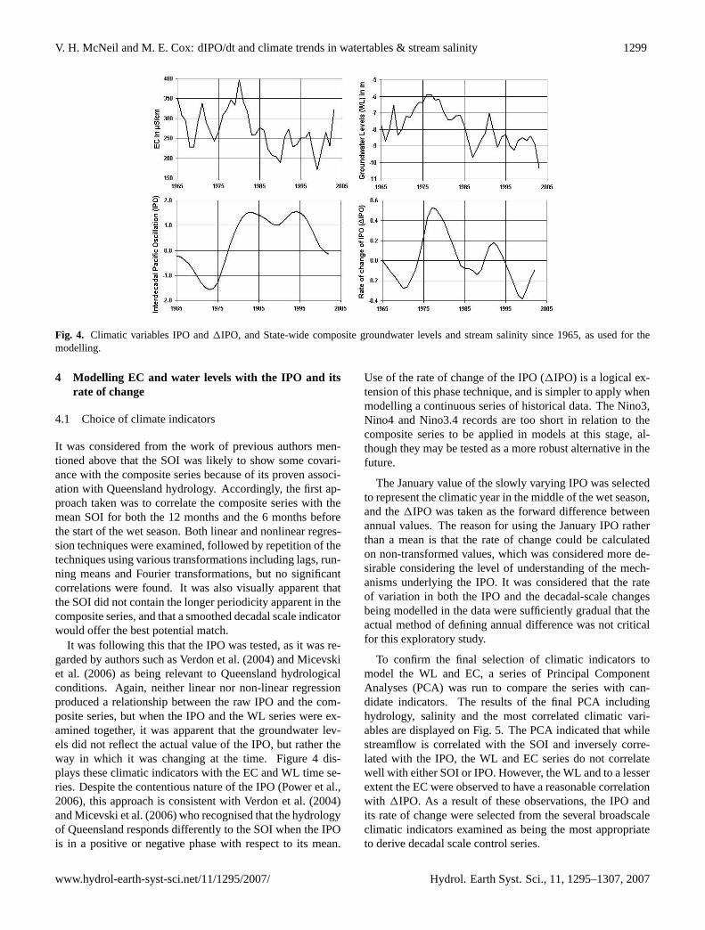
Fig. 4. Climatic variables IPO and1IPO, and State-wide composite groundwater levels and stream salinity since 1965, as used for themodelling.

4 Modelling EC and water levels with the IPO and itsrate of change

4.1 Choice of climate indicators

It was considered from the work of previous authors men-tioned above that the SOI was likely to show some covari-ance with the composite series because of its proven associ-ation with Queensland hydrology. Accordingly, the first ap-proach taken was to correlate the composite series with themean SOI for both the 12 months and the 6 months beforethe start of the wet season. Both linear and nonlinear regres-sion techniques were examined, followed by repetition of thetechniques using various transformations including lags, run-ning means and Fourier transformations, but no significantcorrelations were found. It was also visually apparent thatthe SOI did not contain the longer periodicity apparent in thecomposite series, and that a smoothed decadal scale indicatorwould offer the best potential match.

It was following this that the IPO was tested, as it was re-garded by authors such as Verdon et al. (2004) and Micevskiet al. (2006) as being relevant to Queensland hydrologicalconditions. Again, neither linear nor non-linear regressionproduced a relationship between the raw IPO and the com-posite series, but when the IPO and the WL series were ex-amined together, it was apparent that the groundwater lev-els did not reflect the actual value of the IPO, but rather theway in which it was changing at the time. Figure 4 dis-plays these climatic indicators with the EC and WL time se-ries. Despite the contentious nature of the IPO (Power et al.,2006), this approach is consistent with Verdon et al. (2004)and Micevski et al. (2006) who recognised that the hydrologyof Queensland responds differently to the SOI when the IPOis in a positive or negative phase with respect to its mean.

Use of the rate of change of the IPO (1IPO) is a logical ex-tension of this phase technique, and is simpler to apply whenmodelling a continuous series of historical data. The Nino3,Nino4 and Nino3.4 records are too short in relation to thecomposite series to be applied in models at this stage, al-though they may be tested as a more robust alternative in thefuture.

The January value of the slowly varying IPO was selectedto represent the climatic year in the middle of the wet season,and the1IPO was taken as the forward difference betweenannual values. The reason for using the January IPO ratherthan a mean is that the rate of change could be calculatedon non-transformed values, which was considered more de-sirable considering the level of understanding of the mech-anisms underlying the IPO. It was considered that the rateof variation in both the IPO and the decadal-scale changesbeing modelled in the data were sufficiently gradual that theactual method of defining annual difference was not criticalfor this exploratory study.

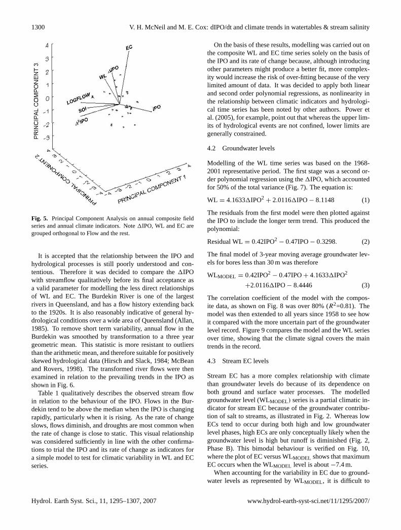
To confirm the final selection of climatic indicators tomodel the WL and EC, a series of Principal ComponentAnalyses (PCA) was run to compare the series with can-didate indicators. The results of the final PCA includinghydrology, salinity and the most correlated climatic vari-ables are displayed on Fig. 5. The PCA indicated that whilestreamflow is correlated with the SOI and inversely corre-lated with the IPO, the WL and EC series do not correlatewell with either SOI or IPO. However, the WL and to a lesserextent the EC were observed to have a reasonable correlationwith 1IPO. As a result of these observations, the IPO andits rate of change were selected from the several broadscaleclimatic indicators examined as being the most appropriateto derive decadal scale control series.



Fig. 5. Principal Component Analysis on annual composite fieldseries and annual climate indicators. Note1IPO, WL and EC aregrouped orthogonal to Flow and the rest.

It is accepted that the relationship between the IPO andhydrological processes is still poorly understood and con-tentious. Therefore it was decided to compare the1IPOwith streamflow qualitatively before its final acceptance asa valid parameter for modelling the less direct relationshipsof WL and EC. The Burdekin River is one of the largestrivers in Queensland, and has a flow history extending backto the 1920s. It is also reasonably indicative of general hy-drological conditions over a wide area of Queensland (Allan,1985). To remove short term variability, annual flow in theBurdekin was smoothed by transformation to a three yeargeometric mean. This statistic is more resistant to outliersthan the arithmetic mean, and therefore suitable for positivelyskewed hydrological data (Hirsch and Slack, 1984; McBeanand Rovers, 1998). The transformed river flows were thenexamined in relation to the prevailing trends in the IPO asshown in Fig. 6.

Table 1 qualitatively describes the observed stream flowin relation to the behaviour of the IPO. Flows in the Bur-dekin tend to be above the median when the IPO is changingrapidly, particularly when it is rising. As the rate of changeslows, flows diminish, and droughts are most common whenthe rate of change is close to static. This visual relationshipwas considered sufficiently in line with the other confirma-tions to trial the IPO and its rate of change as indicators fora simple model to test for climatic variability in WL and ECseries.

On the basis of these results, modelling was carried out onthe composite WL and EC time series solely on the basis ofthe IPO and its rate of change because, although introducingother parameters might produce a better fit, more complex-ity would increase the risk of over-fitting because of the verylimited amount of data. It was decided to apply both linearand second order polynomial regressions, as nonlinearity inthe relationship between climatic indicators and hydrologi-cal time series has been noted by other authors. Power etal. (2005), for example, point out that whereas the upper lim-its of hydrological events are not confined, lower limits aregenerally constrained.

4.2 Groundwater levels

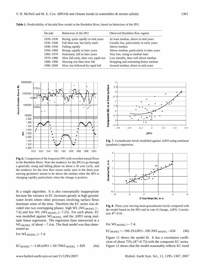
Modelling of the WL time series was based on the 1968-2001 representative period. The first stage was a second or-der polynomial regression using the1IPO, which accountedfor 50% of the total variance (Fig. 7). The equation is:

WL = 4.16331IPO2+ 2.01161IPO− 8.1148 (1)

The residuals from the first model were then plotted againstthe IPO to include the longer term trend. This produced thepolynomial:

Residual WL= 0.42IPO2− 0.47IPO− 0.3298. (2)

The final model of 3-year moving average groundwater lev-els for bores less than 30 m was therefore

WLMODEL = 0.42IPO2− 0.47IPO+ 4.16331IPO2

+2.01161IPO− 8.4446 (3)

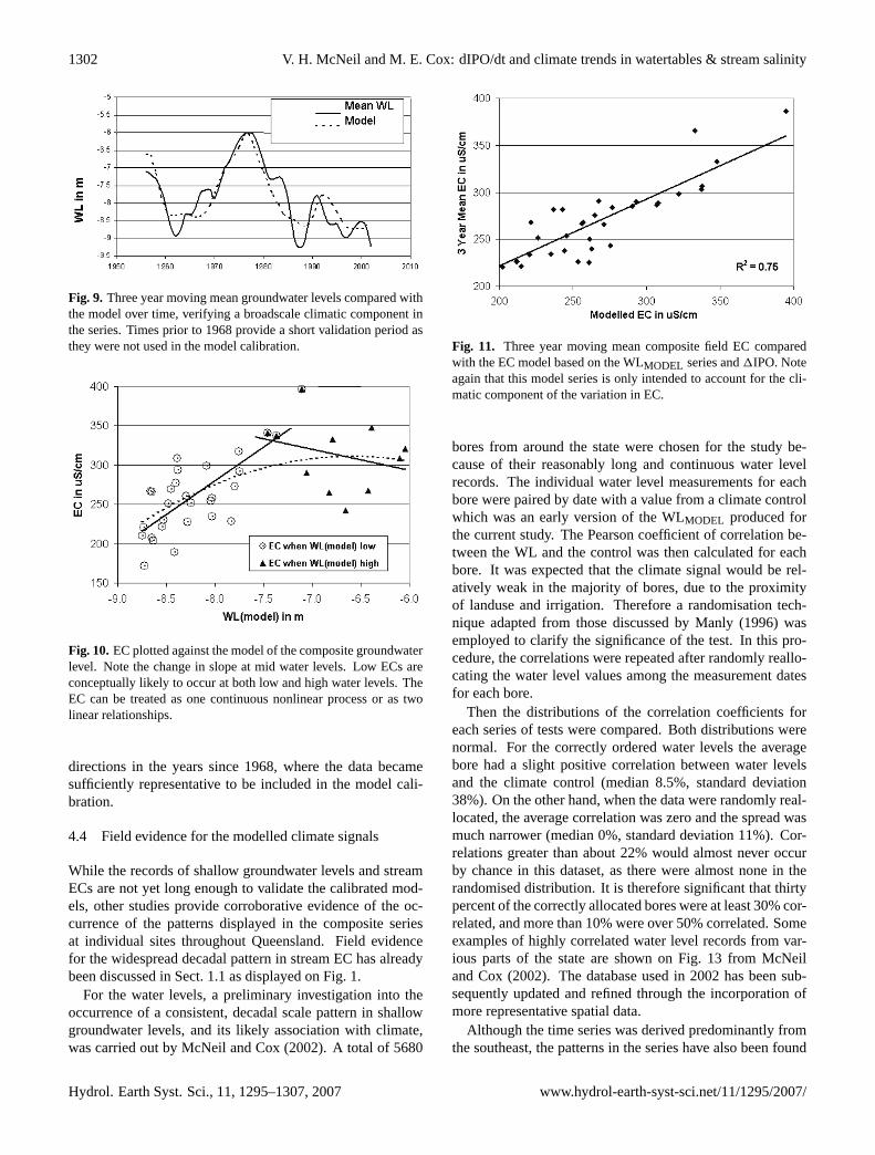
The correlation coefficient of the model with the compos-ite data, as shown on Fig. 8 was over 80% (R2=0.81). Themodel was then extended to all years since 1958 to see howit compared with the more uncertain part of the groundwaterlevel record. Figure 9 compares the model and the WL seriesover time, showing that the climate signal covers the maintrends in the record.

4.3 Stream EC levels

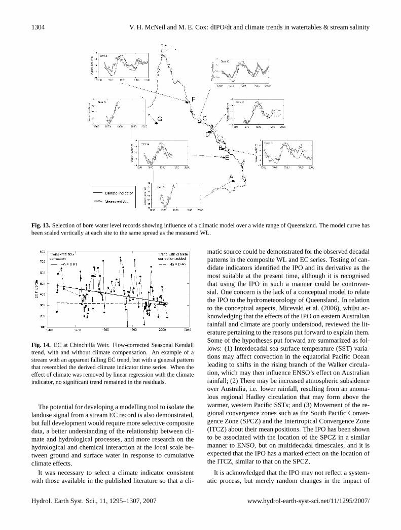
Stream EC has a more complex relationship with climatethan groundwater levels do because of its dependence onboth ground and surface water processes. The modelledgroundwater level (WLMODEL) series is a partial climatic in-dicator for stream EC because of the groundwater contribu-tion of salt to streams, as illustrated in Fig. 2. Whereas lowECs tend to occur during both high and low groundwaterlevel phases, high ECs are only conceptually likely when thegroundwater level is high but runoff is diminished (Fig. 2,Phase B). This bimodal behaviour is verified on Fig. 10,where the plot of EC versus WLMODEL shows that maximumEC occurs when the WLMODEL level is about−7.4 m.

When accounting for the variability in EC due to ground-water levels as represented by WLMODEL, it is difficult to



Table 1. Predictability of decadal flow trends in the Burdekin River, based on behaviour of the IPO.

Decade Behaviour of the IPO Observed Burdekin flow regime

1920–1930 Rising, quite rapidly in mid years At least median, above in mid years1930–1940 Fall then rise, but fairly static Usually low, particularly in early years1940–1950 Falling rapidly Above median1950–1960 Rising, rapidly in later years Above median, particularly in later years1960–1970 Stationary, fall in later years Very low, rising to median later1970–1980 Slow fall early, then very rapid rise Low initially, then well above median1980–1990 Slowing rise then slow fall Dropping and remaining below median1990–2000 Slow rise followed by rapid fall Around median, driest in mid years

Fig. 6. Comparison of the long term IPO with recorded annual flowsin the Burdekin River. Note the tendency for the IPO to go througha generally rising and falling phase on about a 50 year cycle, andthe tendency for the river flow (most easily seen in the three-yearmoving geometric mean) to be above the median when the IPO ischanging rapidly, particularly when the change is positive.

fit a single algorithm. It is also conceptually inappropriatebecause the variance in EC increases greatly at high ground-water levels where other processes involving surface flowsdominate some of the time. Therefore the EC series was di-vided into two overlapping phases: high WL (WLMODEL≥–7.6) and low WL (WLMODEL≤–7.25). For each phase, ECwas modelled against WLMODEL and the1IPO using mul-tiple linear regression. The regression lines intersected at aWLMODEL of about−7.4 m. The final model was thus deter-mined as:

For WLMODEL≤–7.4:

ECMODEL=−5.861IPO+ 69.79WLMODEL + 829 (4a)

Fig. 7. Groundwater levels modelled against1IPO using nonlinear(quadratic) regression.

Fig. 8. Three-year moving mean groundwater levels compared withthe model based on the IPO and its rate of change,1IPO. Correla-tion R2=0.81.

For WLMODEL>–7.4:

ECMODEL=−106.291IPO−106.3WLMODEL−434 (4b)

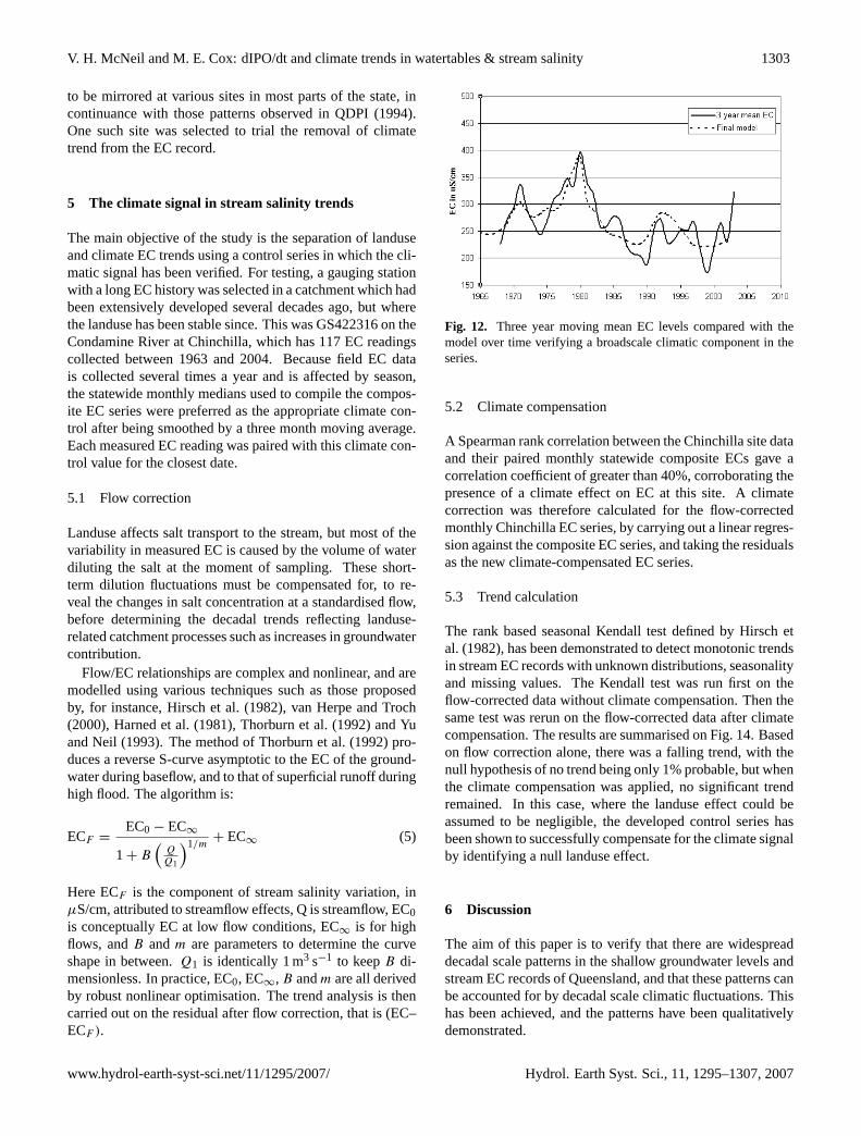
Figure 11 shows the model fit. It has a correlation coeffi-cient of about 75% (R2=0.75) with the composite EC series.Figure 12 shows that the model reasonably reflects EC trend



Fig. 9. Three year moving mean groundwater levels compared withthe model over time, verifying a broadscale climatic component inthe series. Times prior to 1968 provide a short validation period asthey were not used in the model calibration.

Fig. 10.EC plotted against the model of the composite groundwaterlevel. Note the change in slope at mid water levels. Low ECs areconceptually likely to occur at both low and high water levels. TheEC can be treated as one continuous nonlinear process or as twolinear relationships.

directions in the years since 1968, where the data becamesufficiently representative to be included in the model cali-bration.

4.4 Field evidence for the modelled climate signals

While the records of shallow groundwater levels and streamECs are not yet long enough to validate the calibrated mod-els, other studies provide corroborative evidence of the oc-currence of the patterns displayed in the composite seriesat individual sites throughout Queensland. Field evidencefor the widespread decadal pattern in stream EC has alreadybeen discussed in Sect. 1.1 as displayed on Fig. 1.

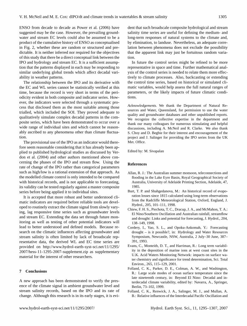
For the water levels, a preliminary investigation into theoccurrence of a consistent, decadal scale pattern in shallowgroundwater levels, and its likely association with climate,was carried out by McNeil and Cox (2002). A total of 5680

Fig. 11. Three year moving mean composite field EC comparedwith the EC model based on the WLMODEL series and1IPO. Noteagain that this model series is only intended to account for the cli-matic component of the variation in EC.

bores from around the state were chosen for the study be-cause of their reasonably long and continuous water levelrecords. The individual water level measurements for eachbore were paired by date with a value from a climate controlwhich was an early version of the WLMODEL produced forthe current study. The Pearson coefficient of correlation be-tween the WL and the control was then calculated for eachbore. It was expected that the climate signal would be rel-atively weak in the majority of bores, due to the proximityof landuse and irrigation. Therefore a randomisation tech-nique adapted from those discussed by Manly (1996) wasemployed to clarify the significance of the test. In this pro-cedure, the correlations were repeated after randomly reallo-cating the water level values among the measurement datesfor each bore.

Then the distributions of the correlation coefficients foreach series of tests were compared. Both distributions werenormal. For the correctly ordered water levels the averagebore had a slight positive correlation between water levelsand the climate control (median 8.5%, standard deviation38%). On the other hand, when the data were randomly real-located, the average correlation was zero and the spread wasmuch narrower (median 0%, standard deviation 11%). Cor-relations greater than about 22% would almost never occurby chance in this dataset, as there were almost none in therandomised distribution. It is therefore significant that thirtypercent of the correctly allocated bores were at least 30% cor-related, and more than 10% were over 50% correlated. Someexamples of highly correlated water level records from var-ious parts of the state are shown on Fig. 13 from McNeiland Cox (2002). The database used in 2002 has been sub-sequently updated and refined through the incorporation ofmore representative spatial data.

Although the time series was derived predominantly fromthe southeast, the patterns in the series have also been found



to be mirrored at various sites in most parts of the state, incontinuance with those patterns observed in QDPI (1994).One such site was selected to trial the removal of climatetrend from the EC record.

5 The climate signal in stream salinity trends

The main objective of the study is the separation of landuseand climate EC trends using a control series in which the cli-matic signal has been verified. For testing, a gauging stationwith a long EC history was selected in a catchment which hadbeen extensively developed several decades ago, but wherethe landuse has been stable since. This was GS422316 on theCondamine River at Chinchilla, which has 117 EC readingscollected between 1963 and 2004. Because field EC datais collected several times a year and is affected by season,the statewide monthly medians used to compile the compos-ite EC series were preferred as the appropriate climate con-trol after being smoothed by a three month moving average.Each measured EC reading was paired with this climate con-trol value for the closest date.

5.1 Flow correction

Landuse affects salt transport to the stream, but most of thevariability in measured EC is caused by the volume of waterdiluting the salt at the moment of sampling. These short-term dilution fluctuations must be compensated for, to re-veal the changes in salt concentration at a standardised flow,before determining the decadal trends reflecting landuse-related catchment processes such as increases in groundwatercontribution.

Flow/EC relationships are complex and nonlinear, and aremodelled using various techniques such as those proposedby, for instance, Hirsch et al. (1982), van Herpe and Troch(2000), Harned et al. (1981), Thorburn et al. (1992) and Yuand Neil (1993). The method of Thorburn et al. (1992) pro-duces a reverse S-curve asymptotic to the EC of the ground-water during baseflow, and to that of superficial runoff duringhigh flood. The algorithm is:

ECF =EC0 − EC∞

1 + B

(

QQ1

)1/m+ EC∞ (5)

Here ECF is the component of stream salinity variation, inµS/cm, attributed to streamflow effects, Q is streamflow, EC0is conceptually EC at low flow conditions, EC∞ is for highflows, andB andm are parameters to determine the curveshape in between.Q1 is identically 1 m3 s−1 to keepB di-mensionless. In practice, EC0, EC∞, B andm are all derivedby robust nonlinear optimisation. The trend analysis is thencarried out on the residual after flow correction, that is (EC–ECF ).

Fig. 12. Three year moving mean EC levels compared with themodel over time verifying a broadscale climatic component in theseries.

5.2 Climate compensation

A Spearman rank correlation between the Chinchilla site dataand their paired monthly statewide composite ECs gave acorrelation coefficient of greater than 40%, corroborating thepresence of a climate effect on EC at this site. A climatecorrection was therefore calculated for the flow-correctedmonthly Chinchilla EC series, by carrying out a linear regres-sion against the composite EC series, and taking the residualsas the new climate-compensated EC series.

5.3 Trend calculation

The rank based seasonal Kendall test defined by Hirsch etal. (1982), has been demonstrated to detect monotonic trendsin stream EC records with unknown distributions, seasonalityand missing values. The Kendall test was run first on theflow-corrected data without climate compensation. Then thesame test was rerun on the flow-corrected data after climatecompensation. The results are summarised on Fig. 14. Basedon flow correction alone, there was a falling trend, with thenull hypothesis of no trend being only 1% probable, but whenthe climate compensation was applied, no significant trendremained. In this case, where the landuse effect could beassumed to be negligible, the developed control series hasbeen shown to successfully compensate for the climate signalby identifying a null landuse effect.

6 Discussion

The aim of this paper is to verify that there are widespreaddecadal scale patterns in the shallow groundwater levels andstream EC records of Queensland, and that these patterns canbe accounted for by decadal scale climatic fluctuations. Thishas been achieved, and the patterns have been qualitativelydemonstrated.



Fig. 13. Selection of bore water level records showing influence of a climatic model over a wide range of Queensland. The model curve hasbeen scaled vertically at each site to the same spread as the measured WL.

Fig. 14. EC at Chinchilla Weir. Flow-corrected Seasonal Kendalltrend, with and without climate compensation. An example of astream with an apparent falling EC trend, but with a general patternthat resembled the derived climate indicator time series. When theeffect of climate was removed by linear regression with the climateindicator, no significant trend remained in the residuals.

The potential for developing a modelling tool to isolate thelanduse signal from a stream EC record is also demonstrated,but full development would require more selective compositedata, a better understanding of the relationship between cli-mate and hydrological processes, and more research on thehydrological and chemical interaction at the local scale be-tween ground and surface water in response to cumulativeclimate effects.

It was necessary to select a climate indicator consistentwith those available in the published literature so that a cli-

matic source could be demonstrated for the observed decadalpatterns in the composite WL and EC series. Testing of can-didate indicators identified the IPO and its derivative as themost suitable at the present time, although it is recognisedthat using the IPO in such a manner could be controver-sial. One concern is the lack of a conceptual model to relatethe IPO to the hydrometeorology of Queensland. In relationto the conceptual aspects, Micevski et al. (2006), whilst ac-knowledging that the effects of the IPO on eastern Australianrainfall and climate are poorly understood, reviewed the lit-erature pertaining to the reasons put forward to explain them.Some of the hypotheses put forward are summarized as fol-lows: (1) Interdecadal sea surface temperature (SST) varia-tions may affect convection in the equatorial Pacific Oceanleading to shifts in the rising branch of the Walker circula-tion, which may then influence ENSO’s effect on Australianrainfall; (2) There may be increased atmospheric subsidenceover Australia, i.e. lower rainfall, resulting from an anoma-lous regional Hadley circulation that may form above thewarmer, western Pacific SSTs; and (3) Movement of the re-gional convergence zones such as the South Pacific Conver-gence Zone (SPCZ) and the Intertropical Convergence Zone(ITCZ) about their mean positions. The IPO has been shownto be associated with the location of the SPCZ in a similarmanner to ENSO, but on multidecadal timescales, and it isexpected that the IPO has a marked effect on the location ofthe ITCZ, similar to that on the SPCZ.

It is acknowledged that the IPO may not reflect a system-atic process, but merely random changes in the impact of



ENSO from decade to decade as Power et al. (2006) havesuggested may be the case. However, the prevailing ground-water and stream EC levels could also be assumed to be aproduct of the cumulative history of ENSO as conceptualisedin Fig. 2, whether these are random or structured and pre-dictable. It is neither inferred nor required for the objectivesof this study that there be a direct conceptual link between theIPO and hydrology and stream EC. It is a sufficient assump-tion that the patterns displayed in each may be responding tosimilar underlying global trends which affect decadal vari-ability in weather patterns.

The relationship between the IPO and its derivative withthe EC and WL series cannot be statistically verified at thistime, because the record is very short in terms of the peri-odicity evident in both composite and indicator series. How-ever, the indicators were selected through a systematic pro-cess that disclosed them as the most suitable among thosetrialled, which included the SOI. They proved adequate toqualitatively simulate complex decadal patterns in the com-posite series, which have been demonstrated to occur over awide range of individual sites and which cannot be reason-ably ascribed to any phenomena other than climate fluctua-tion.

The provisional use of the IPO as an indicator would there-fore seem reasonable considering that it has already been ap-plied to published hydrological studies as discussed by Ver-don et al. (2004) and other authors mentioned above con-cerning the phases of the IPO and stream flow. Using therate of change of the IPO rather than categorical parameterssuch as high/low is a rational extension of that approach. Asthe modelled climate control is only intended to be comparedwith historical records, and is not applicable to forecasting,its validity can be tested regularly against a master compositeseries before being applied it to individual sites.

It is accepted that more robust and better understood cli-matic indicators are required before reliable tools are devel-oped to routinely extract the climate signal from slowly vary-ing, lag responsive time series such as groundwater levelsand stream EC. Extending the data set through future mon-itoring as well as testing of other potential indicators willlead to better understood and defined models. Because re-search on the climatic influences affecting groundwater andstream salinity is often limited by lack of broadscale rep-resentative data, the derived WL and EC time series areprovided on http://www.hydrol-earth-syst-sci.net/11/1295/2007/hess-11-1295-2007-supplement.zip as supplementarymaterial for the interest of other researchers.

7 Conclusions

A new approach has been demonstrated to verify the pres-ence of the climate signal in ambient groundwater level andstream salinity records, based on the IPO and its rate ofchange. Although this research is in its early stages, it is evi-

dent that such broadscale composite hydrological and streamsalinity time series are useful for defining the medium- andlong-term responses of natural systems to the climate and,by elimination, to landuse. Nevertheless, an adequate corre-lation between phenomena does not exclude the possibilitythat the apparent link may just be fortuitous random varia-tion.

In future the control series might be refined to be morerepresentative in space and time. Further mathematical anal-ysis of the control series is needed to relate them more effec-tively to climate processes. Also, backcasting or extendingthe control time series, based on historical or simulated cli-matic variables, would help assess the full natural ranges ofparameters, or the likely impacts of future climatic condi-tions.

Acknowledgements. We thank the Department of Natural Re-sources and Water, Queensland, for permission to use the waterquality and groundwater databases and other unpublished reports.We recognize the collective expertise in the department andthank our many colleagues for numerous stimulating and helpfuldiscussions, including A. McNeil and R. Clarke. We also thankS. Choy and D. Begbie for their interest and encouragement of theproject and J. Salinger for providing the IPO series from the UKMet. Office.

Edited by: M. Sivapalan

References

Allan, R. J.: The Australian summer monsoon, teleconnections andflooding in the Lake Eyre Basin, Royal Geographical Society ofAustralia, University of Adelaide Printing Section, Adelaide, 47,1985.

Burt, T. P. and Shahgedanova, M.: An historical record of evapo-ration losses since 1815 calculated using long-term observationsfrom the Radcliffe Meteorological Station, Oxford, England, J.Hydrol., 205, 101–111, 1998.

Chiew, F. H. S., Piechota, T. C., Dracup, J. A., and McMahon, T. A.:El Nino/Southern Oscillation and Australian rainfall, streamflowand drought: Links and potential for forecasting, J. Hydrol., 204,138–149, 1998.

Cordery, I., Yao, S. L., and Opoku-Ankomah, Y.: Forecastingdrought – is it possible?, in: Hydrology and Water ResourcesSymposium, Newcastle, NSW, Australia, 2 July–30 June, 387–391, 1993.

Evans, C., Monteith, D. T., and Harriman, R.: Long term variabil-ity in the deposition of marine ions at west coast sites in theU.K. Acid Waters Monitoring Network: impacts on surface wa-ter chemistry and significance for trend determination, Sci. TotalEnviron., 265, 115–129, 2001.

Folland, C. K., Parker, D. E., Colman, A. W., and Washington,R.: Large scale modes of ocean surface temperature since thelate nineteenth century, in: Beyond El Nino: Decadal and in-terdecadal climate variability, edited by: Navarra, A., Springer,Berlin, 73–102, 1999.

Folland, C. K., Renwick, J. A., Salinger, M. J., and Mullan, A.B.: Relative influences of the Interdecadal Pacific Oscillation and


http://www.hydrol-earth-syst-sci.net/11/1295/2007/hess-11-1295-2007-supplement.zip

http://www.hydrol-earth-syst-sci.net/11/1295/2007/hess-11-1295-2007-supplement.zip


ENSO in the South Pacific Convergence Zone, Geophys. Res.Lett., 29, 21.21–21.24, 2002a.

Folland, C. K., Salinger, M. J., Jiangand, N., and Rayner, N. A.:Trends and variations in south pacific island and ocean surfacetemperatures, J. Climate, 16, 2859–2874, 2002b.

Franks, S. W.: Identification of a change in climate state using re-gional flood data, Hydrol. Earth Syst. Sci., 6, 11–16, 2002,http://www.hydrol-earth-syst-sci.net/6/11/2002/.

Gellens, D. and Roulin, E.: Streamflow response of Belgian catch-ments to IPCC climate change scenarios, J. Hydrol., 210, 242–258, 1998.

Gordon, N. D.: The Southern Oscillation and New Zealand weather,Mon. Wea. Rev., 114, 371–387, 1986.

Gray, W. M.: Strong association between West African rainfalland U.S. landfall of intense hurricanes, Sci. Total Environ., 249,1251–1256, 1990.

Harned, D. A., Daniel, C. C., and Crawford, J. K.: Methods of dis-charge compensation as an aid to the evaluation of water qualitytrends, Water Resour. Res., 17, 1389–1400, 1981.

Henderson, K. A., Thompson, L. G., and Lin, P. N.: Recording ofEl Nino in ice core d18O records from Nevado Huascaran, Peru,J. Geophys. Res., 104, 31 053–31 065, 1990.

Hirsch, R. M., Slack, J. R., and Smith, R. A.: Techniques of trendanalysis for monthly water quality data, Water Resour. Res., 18,107–121, 1982.

Hirsch, R. M. and Slack, J. A: A nonparametric test for seasonaldata and seasonal dependence, Water Resour. Res., 20, 727–732,1984.

IPCC: Report of the Intergovernmental Panel on Climate Change,edited by: Houghton, J. T., Callander, B. A., and Varney, S. K.,Cambridge University Press, Cambridge, UK, 1996.

Jolly, P. B. and Chin, D. N.: Long term rainfall – recharge relation-ships within the Northern Territory, Australia, in: InternationalHydrology and Water Resources Symposium: The foundationfor sustainable development, Perth, W. A., Australia, 2–4 Octo-ber 1991.

Jones, K. and Everingham, Y.: Can ENSO combined with Low-Frequency SST signals enhance or suppress rainfall in Australiansugar growing areas?, in: MODSIM 2005 International Congresson Modelling and Simulation, edited by: Zerger, A. and Argent,R. M., Melbourne, December, Modelling and Simulation Societyof Australia and New Zealand, 1660–1666, 2005.

Kahya, E. and Dracup, J. A.: U.S. streamflow patterns in relation tothe El Nino/Southern Oscillation, Water Resour. Res., 29, 2491–2503, 1993.

Kiem, A. S., Franks, S. W., and Kuczera, G.: Multi-decadal vari-ability of flood risk, Geophys. Res. Lett., 30, 1035, Online accessdoi:1010.1029/2002GL015992, 012003.015999, 2002.

Kiem, A. S. and Franks, S. W.: Multi-decadal variability of droughtrisk, eastern Australia, Hydrol. Processes, 18, 2039–2050, 2004.

Loewe, F. and Radok, U.: Variability and periodicity of meteoro-logical elements in the southern hemisphere with particular ref-erence to Australia. Canberra, A.C.T., Commonwealth Meteoro-logical Bureau, Meteorological Branch, Dept. of Interior, Com-monwealth of Australia. 49, 1948.

Lough, J. M.: Rainfall variations in Queensland. Australia: 1891–1986, Int. J. Climatol., 11, 745–768, 1991.

McBean, E. A. and Rovers, F. A.: Statistical procedures for analy-sis of environmental monitoring data and risk assessment, Upper

Saddle River, New Jersey, Prentice Hall, 1998.McBride, J. L. and Nicholls, N.: Seasonal relationships between

Australian rainfall and the Southern Oscillation, Mon. Wea. Rev.,111, 1998–2004, 1983.

McKeon, G. M., Hall, W. B., Henry, B. K., Stone, G. S., and Wat-son, I. W.: Pasture degradation and recovery in Australia’s range-lands: Learning from History, Queensland Department of Natu-ral Resources, Mines and Energy, 2004.

McKerchar, A. I., Pearson, C. P., and Moss, M. E.: Prediction ofsummer inflows to lakes in the Southern Alps, New Zealand, J.Hydrol, 184, 175–187, 1996.

McKerchar, A. I., Pearson, C. P., and Fitzharris, B. B.: Dependencyof summer lake inflows and precipitation on spring SOI, J. Hy-drol., 205, 66–80, 1998.

McNeil, V. H. and Cox, M. E.: Relationships between recent cli-mate variation and water tables on stream salinity trends in north-ern Australia, in: IAH International Groundwater Conference,Balancing the groundwater budget, 12–17 May, Darwin, North-ern Territory, 2002.

McNeil, V. H., Cox, M. E., and Preda, M.: Assessment of chemicalwater types and their spatial variation using multi-stage clusteranalysis, Queensland, Australia, J. Hydrol., 310, 181–200, 2005.

Manly, B. F. J.: Randomisation, bootstrap and Monte Carlo meth-ods in biology, Chapman and Hall, London, 1997.

Micevski, T., Franks, S. W., and Kuczera, G.: Multidecadal vari-ability in coastal eastern Australian flood data, J. Hydrol., 327(1–2), 219–225, 2006.

Mullan, A. B.: On the linearity and stability of SouthernOscillation-climate relationships for New Zealand, Int. J. Clima-tol., 15, 1365–1386, 1995.

Nicholls, N.: ENSO and rainfall variability, J. Climate, 1, 418–421,1988.

Philander, S. G. H.: El Nino, La Nina and the Southern Oscillation.Academic Press, San Diego, 1990.

Power, S., Tseitkin, F., Torok, S., Lavery, B., Dahni, R., and McA-vaney, B.: Australian temperature, Australian rainfall and theSouthern Oscillation, 1910–1992: coherent variability and recentchanges, Aust. Meteorol. Mag., 47, 85–101, 1998.

Power, S., Casey, T., Folland, C., Colman, A., and Mehta, V.: Inter-decadal modulation of the impact of ENSO on Australia, Clim.Dyn., 15, 319–324, 1999.

Power, S., Haylock, M., Colman, R., and Wang, X.: Asymmetry inthe Australian response to ENSO and the predictability of inter-decadal changes in ENSO teleconnections, Bureau of Meteorol-ogy, Melbourne, Australia, 65, 2005.

Power, S., Haylock, M., Colman, R., and Wang, X.: ThePredictability of Interdecadal Changes in ENSO Activityand ENSO Teleconnections, J. Climate, 19(19), 4755–4771doi:10.1175/JCLI3868.1, 2006.

QDPI: Queensland Water Quality Atlas. Queensland Department ofPrimary Industries, Brisbane, 1994.

Ropelewski, C. F. and Halpert, M. S.: Global and regional scaleprecipitation patterns associated with the El Nino/Southern Os-cillation, Mon. Wea. Rev., 115, 1606–1626, 1987.

Ropelewski, C. F. and Halpert, M. S.: Precipitation patterns asso-ciated with the high index phase of the Southern Oscillation, J.Climate, 2, 268–284, 1989.

Rowell, D. P. and Zwiers, F. W.: The global distribution of sourcesof atmospheric decadal variability and mechanisms over the trop-


http://www.hydrol-earth-syst-sci.net/6/11/2002/


ical Pacific and southern North America, Clim. Dyn., 15, 751–772, 1999.

Ruprecht, J. K. and Schofield, N. J.: Effects of partial deforesta-tion on hydrology and salinity in high salt storage landscapes, I:extensive block clearing, J. Hydrol, 129, 19–38, 1991.

Salinger, M. J., Renwick, J. A., and Mullan, A. B.: InterdecadalPacific Oscillation and South Pacific climate, Int. J. Climatol.,21, 1705–1721, 2001.

Thorburn, P., Shaw, R., and Gordon, I.: Modelling salt transport inthe landscape. In Modelling chemical transport in soils, editedby: Ghadiri, H. and Rose, C. W., CRC Pres, 180–189, 1992.

Troup, A. J.: The Southern Oscillation, Quart. J. Roy. Meteorol.Soc., 91, 490–506, 1965.

Vaccaro, J. J.: Sensitivity of groundwater recharge estimates to cli-mate variability and change, Columbia Plateau, Washington, J.Geophys. Res., 97, 2821–2833, 1993.

van Herpe, Y. and Troch, P. A.: Spatial and temporal variations innitrate concentrations in a mixed land use catchment under hu-mid temperate climatic conditions, Hydrol. Processes, 14, 2439–2455, 2000.

Verdon, D. C., Wyatt, A. M., Kiem, A. S., and Franks, S. W.: Multi-decadal variability of rainfall and streamflow: Eastern Australia,Water Resour. Res., 40, W10201, doi:10.1029/2004WR003234,2004.

Yu, B. and Neil, D. T.: Salinity trend of the Williams River, WesternAustralia, J. Roy. Soc. Western Australia, 76, 71–76, 1993.

Zhang, Y., Wallace, J. M., and Battisti, D. S.: ENSO-like inter-decadal variability: 1900–93, J. Climate, 10, 1004–1020, 1997.

Zorn, M. H. and Waylen, P. R.: Seasonal response of mean monthlystreamflow to El Nino/Southern Oscillation in North CentralFlorida, Prof. Geogr., 49, 51–62, 1997.


Documents

De ning the climatic signal in stream salinity trends