Embed Size (px)
Citation preview
Defining Racial and Ethnic Context with Geolocation Data∗
forthcoming Political Science Research and Methods
Ryan T. Moore† Andrew Reeves‡
January 20, 2020
Abstract
Across disciplines, scholars strive to better understand individuals’ milieus—the people,places, and institutions individuals encounter in their daily lives. In particular, political sci-entists argue that racial and ethnic context shapes attitudes about candidates, policies, andfellow citizens. Yet the current standard of measuring milieus is to place survey respondentsin a geographic container and then to ascribe all that container’s characteristics to the individ-ual’s milieu. Using a new dataset of over 2.6 million GPS records from over 400 individuals,we compare conventional static measures of racial and ethnic context to dynamic, precise mea-sures of milieus. We demonstrate how low-level static measures tend to overstate how extremeindividuals’ racial and ethnic contexts are, and offer suggestions for future researchers.
∗All data and information necessary to replicate the results in this article are available in the Harvard Dataverse atMoore and Reeves (2020) at https://doi.org/10.7910/DVN/G3YJXY. We thank Brady Baybeck, Michael Kellermann,Melissa Sands, Allen Settle, Stuart Soroka, Steven Webster, and participants of the Toronto Political BehaviourWorkshop, the Women’s and Minority Representation conference of McGill University’s Centre for the Study ofDemocratic Citizenship, and the American University Government Research Seminar for comments and suggestionson earlier drafts.†Department of Government, American University, Ward Circle Building 226, 4400 Massachusetts Av-
enue NW, Washington DC 20016-8130. tel: 202.885.6470; fax: 202.885.2967; rtm (at) american (dot) edu;http://www.ryantmoore.org.‡Associate Professor, Department of Political Science Washington University in St. Louis, Campus Box 1063, One
Brookings Drive, St. Louis MO 63130, http://www.andrewreeves.org, [email protected], (314) 935-8427.
1
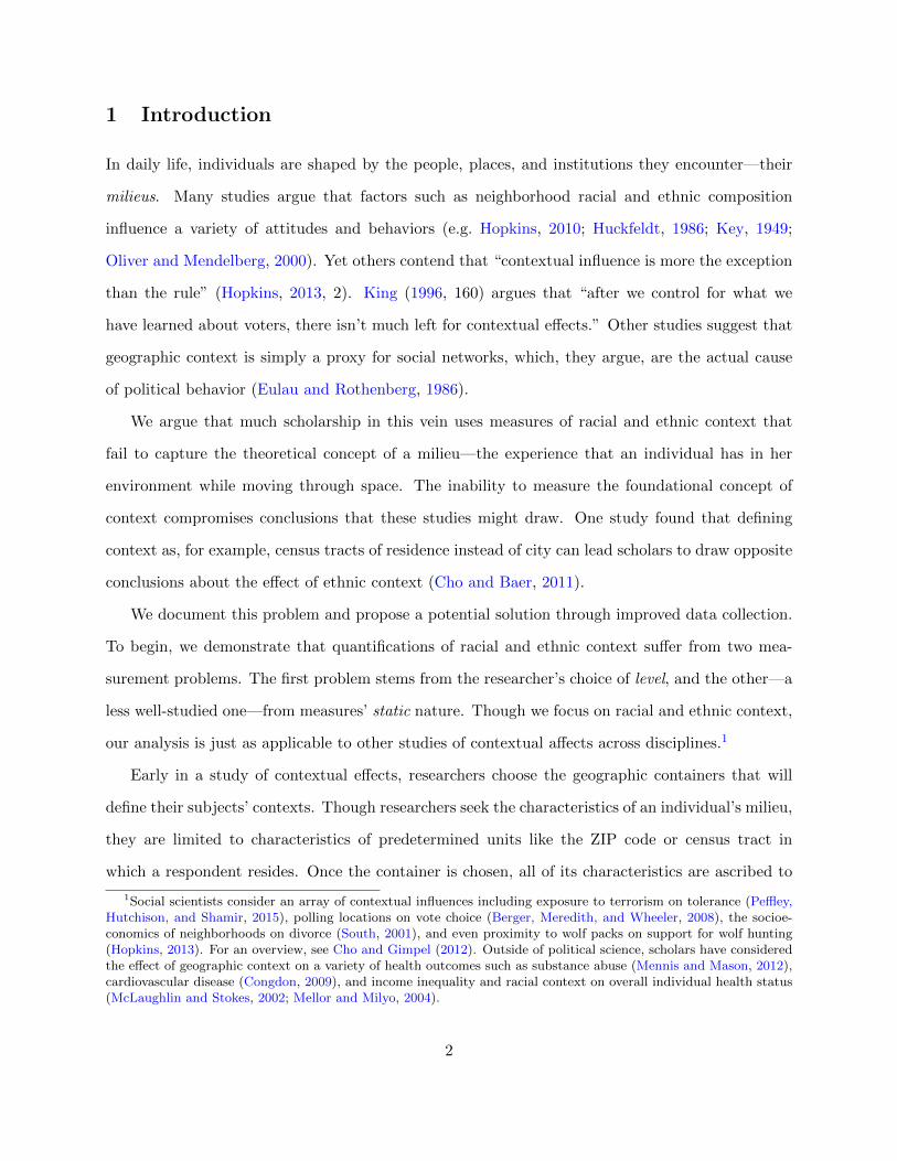
1 Introduction
In daily life, individuals are shaped by the people, places, and institutions they encounter—their
milieus. Many studies argue that factors such as neighborhood racial and ethnic composition
influence a variety of attitudes and behaviors (e.g. Hopkins, 2010; Huckfeldt, 1986; Key, 1949;
Oliver and Mendelberg, 2000). Yet others contend that “contextual influence is more the exception
than the rule” (Hopkins, 2013, 2). King (1996, 160) argues that “after we control for what we
have learned about voters, there isn’t much left for contextual effects.” Other studies suggest that
geographic context is simply a proxy for social networks, which, they argue, are the actual cause
of political behavior (Eulau and Rothenberg, 1986).
We argue that much scholarship in this vein uses measures of racial and ethnic context that
fail to capture the theoretical concept of a milieu—the experience that an individual has in her
environment while moving through space. The inability to measure the foundational concept of
context compromises conclusions that these studies might draw. One study found that defining
context as, for example, census tracts of residence instead of city can lead scholars to draw opposite
conclusions about the effect of ethnic context (Cho and Baer, 2011).
We document this problem and propose a potential solution through improved data collection.
To begin, we demonstrate that quantifications of racial and ethnic context suffer from two mea-
surement problems. The first problem stems from the researcher’s choice of level, and the other—a
less well-studied one—from measures’ static nature. Though we focus on racial and ethnic context,
our analysis is just as applicable to other studies of contextual affects across disciplines.1
Early in a study of contextual effects, researchers choose the geographic containers that will
define their subjects’ contexts. Though researchers seek the characteristics of an individual’s milieu,
they are limited to characteristics of predetermined units like the ZIP code or census tract in
which a respondent resides. Once the container is chosen, all of its characteristics are ascribed to
1Social scientists consider an array of contextual influences including exposure to terrorism on tolerance (Peffley,Hutchison, and Shamir, 2015), polling locations on vote choice (Berger, Meredith, and Wheeler, 2008), the socioe-conomics of neighborhoods on divorce (South, 2001), and even proximity to wolf packs on support for wolf hunting(Hopkins, 2013). For an overview, see Cho and Gimpel (2012). Outside of political science, scholars have consideredthe effect of geographic context on a variety of health outcomes such as substance abuse (Mennis and Mason, 2012),cardiovascular disease (Congdon, 2009), and income inequality and racial context on overall individual health status(McLaughlin and Stokes, 2002; Mellor and Milyo, 2004).
2
the respondent as her contextual experience. Sometimes these containers are small, like a single
census block group, and other times they are expansive, like an entire state. Small geographies
may arbitrarily constrain an individual’s measures to a few city blocks, while large geographies
unrealistically assume an individual experiences an entire state. Even the smallest state is hundreds
of thousands of times larger than a city block, yet studies pick either container to measure the same
context. Often, decisions about which container to use may be “choices driven by convenience and
data availability”(Cho and Baer, 2011, 418).
Recent research in measuring racial and ethnic context deepens our understanding of perceptions
versus objective measures (Hjorth, Dinesen, and Sønderskov, 2016; Velez and Wong, 2016; Wong
et al., 2013, 2015, 2016, 2012) and overlapping residential communities (Baybeck, 2006). However,
we argue that even those researchers interested in objective rather than perceptual measures should
employ individualized, precise, dynamic measures when possible. Below, we review approaches to
measuring different contexts, arguing that traditional measures can be systematically misleading.
Section 3 presents original individual-level geolocation data from over 400 individuals that we began
recruiting in July 2013. Section 4 shows how the natural variation in individual experiences in our
data belies static, aggregate measures. We evaluate particular levels of geographic aggregation
and provide advice for scholars without access to dynamic measures. Finally, we detail the large
individual variation in geographic context, even within particular American metropolitan areas.
2 Measuring Racial and Ethnic Context
Existing census measures of racial and ethnic context have limited decades of studies to using static
geographic containers. As a result, measures of context may significantly misrepresent the local
dynamic experiences that are posited to influence individuals’ political behaviors and attitudes.
Many applications measure context at the county level, for example.2 However, the demographics
and political environment of a respondent’s county may differ greatly from those of the part of
the county she actually lives in, works in, drives through, or experiences during her day. American
2We count our own work among these studies (e.g. Gasper and Reeves, 2011; Kriner and Reeves, 2012, 2015;Moore and Ravishankar, 2012).
3
counties are as large as 20,000 square miles—San Bernadino County, California, is larger than Costa
Rica, Bosnia and Herzegovina, and Denmark—and encapsulate many different kinds of areas. As
such, county-level averages likely misrepresent the experiences of many individuals. The average
county includes about 1000 square miles; an average measure taken over a 50-mile by 20-mile area
will significantly distort many individual experiences. We show several examples in Section 5.
Contextual factors are hypothesized to drive a number of attitudes related to prejudice. One
seminal theoretic divide is whether in-group interactions with out-group members increase hostility
or empathy toward the out-group. For example, (Dinesen and Sønderskov, 2015, 550) find that
“residential exposure to ethnic diversity reduces social trust”. This work frequently uses static
geographic containers including counties (Dixon, 2006; Fosset and Kiecolt, 1989; Giles and Evans,
1986; Glaser, 1994; Stein, Post, and Rinden, 2000; Taylor, 1998); cities or standard metropolitan
statistical areas (SMSAs) (Bledsoe et al., 1995; Dixon, 2006; Fosset and Kiecolt, 1989; Oliver and
Wong, 2003; Oliver and Mendelberg, 2000; Taylor, 1998); and states (Hero and Tolbert, 2004).
Lower levels of geography are also used, including housing projects (Ford, 1973), ZIP codes (Cho
and Baer, 2011; Gilliam, Valentino, and Beckmann, 2002; Oliver and Mendelberg, 2000; Weber
et al., 2014), and neighborhoods (Bledsoe et al., 1995; Cho and Baer, 2011; Stolle, Soroka, and
Johnston, 2008). Rarely, very low levels such as census blocks are used (Oliver and Wong, 2003). As
we show, each of these containers consistently mismeasures context when compared to individuals’
actual dynamic experiences.3
Geographic contexts have also been connected to other political behaviors, such as state to
turnout (Solt, 2010), neighborhood to turnout (Cho, Gimpel, and Dyck, 2006), county to views on
Ronald Reagan (MacKuen and Brown, 1987), cities and census blocks to attitudes toward local
government and one’s neighborhood (Baybeck, 2006), and neighborhood to various forms of partic-
ipation (Huckfeldt, 1979). Mutz and Mondak (2006) compares the workplace as a locus of political
discussion with other contexts like the neighborhood and household. Baybeck and Huckfeldt (2002)
and Berry and Baybeck (2005) deploy GIS data to demonstrate that geographic distance strongly
3Studies also address how characteristics of a place change over time (e.g., Green, Strolovitch, and Wong, 1998;Hopkins, 2010). While we do not address the temporal dimension of an individual’s milieu here, it merits furtherstudy. Others also relate context to political behaviors such as voting for California’s immigration Proposition 187(Morris, 2000), for George Wallace for president (Wright, 1976), and for a black mayoral candidate (Carsey, 1995).
4
predicts the density of political discussion networks and that interstate competition drives lottery
adoptions (but not welfare benefit levels), respectively.
A small body of research takes a more circumspect approach to conceptualizing their measures
of geography (Cho and Baer, 2011; Christiansen, Sønderskov, and Dinesen, 2016; Gimpel et al.,
Forthcoming; Reeves and Gimpel, 2012; Wong et al., 2013). Analyzing economic attitudes, Reeves
and Gimpel (2012) considers states, media markets, and counties, and then constructs multiple
geographic regions based on social, political, and economic similarities of adjacent counties. Chris-
tiansen, Sønderskov, and Dinesen (2016) argues that national economic perceptions are driven by
extremely local conditions—unemployment rates within 80 meters of home, but not unemployment
within larger radii, such as 2500 meters. Cho and Baer (2011) analyzes racial attitudes of blacks
as a function of, among other things, multiple measures of racial context including census tract,
ZIP code, neighborhood, and city. The study finds that the proportion of Latinos in a respondent’s
census tract is negatively associated with attitudes toward Latinos; however these same attitudes
are positively associated with the proportion of Latinos measured at the city level. Using ZIP code
or neighborhood measures yields statistically insignificant relationships between the same variables.
Cho and Baer (2011) then shows that incorporating nearby census tracts (as well as a measure of
socioeconomic status) yields consistent results across geographic levels. Cho, Gimpel, and Shaw
(2012) similarly employs nearby geographic units in their spatial analyses.
The important finding of Cho and Baer (2011) is consistent with our work here, but there
are differences. First, our sample here is geographically broader, touching every American state.
Second, we dynamically measure the racial and ethnic milieus through which individuals actually
pass, rather than statically assign them to a single set of nested geographic containers. Third, the
lowest level of geography we employ is the census block, of which there are about 200 times as
many as ZIP codes.
Even work that considers multiple levels of geography assumes that static measures—whatever
their level—capture racial or economic experiences. As we demonstrate below, static measures of
any level may not capture dynamic contexts, such as those of two people who live in the same
block, but travel through different parts of a city during their daily lives.
5
We build on work in geography by Kwan (e.g., 2009, 2012) which asserts that contextual
measures of exposure should be “people-based”, rather than “place-based”. Kwan argues that
environmental influences on health and behavior unfold over the course of the day and depend on
the places passed through, rather than being defined by the single place we live. This holds whether
we define where we live broadly, as in a U.S. state, or narrowly, as in a single census block.
2.1 How Aggregate Census Measures Obscure Static Locations
Large geographies could represent their smaller constituent geographies quite well. For example,
if a county were 60% white, each of the census blocks within that county could also be 60%
white. However, larger geographies can also significantly misrepresent the demographics individuals
encounter within them. A county that was 60% white could be a mixture of census blocks that were
100% white and 0% white. Further, where the county average misrepresents the nature of many
blocks, we would not expect very different blocks to lie next to each other. American residential
segregation (Massey and Denton, 1993) implies that demographically similar blocks are likely to
cluster. Thus, where block demographics vary within a county, we expect county measures to be a
poor representation of individuals’ much more localized experiences.4
For example, consider the city of Saint Louis, Missouri. The city is 48.5% black, but 35% of
the city’s census blocks are over 90% white or black.5 If an individual were to experience all census
blocks in the city, then 48.5% could be an accurate measure of her racial milieu. However, if she
remained primarily in homogeneous black or white census blocks, then this summary measure would
be a misleading characterization of her interaction with other racial groups. To address this, we
define context dynamically, based on the characteristics of the areas through which an individual
travels.
2.2 Toward Low-level, Dynamic Measures of Geography
Consider datasets commonly employed in social scientific research and the static geographic iden-
tifiers they sometimes make available. The American National Election Studies (ANES) makes
4For related critiques of standard measures of contextual effects, see Kwan (2009); Matthews (2008).5Of St. Louis’s 9,577 census blocks, 1,315 are over 90% white while 2,023 are over 90% black.
6
available state and Congressional district indicators; it restricts access to county and ZIP code.
The Cooperative Congressional Election Study (CCES) includes respondent region, state, county,
Congressional district, and ZIP code, but ZIP code is missing for 60% of the sample in 2011. The
General Social Survey (GSS) provides respondent region, but restricts access to census tract, as well
as to higher levels of aggregation, including state, standard metropolitan statistical area (SMSA),
and county.
By contrast, consider the geographic experience of the two individuals whose travels are plotted
in Figure 1. These are two real people both of whom were observed in Los Angeles County,
California, from data we describe in Section 3. The two individuals occupy strikingly different
parts of the county—information that would be completely obscured by static measures of county.
Despite both living in Los Angeles County, their milieus are distinct. Person 1, whose path is
plotted with grey triangles (4), primarily occupies the West Los Angeles area. Person 2, whose
path is plotted with black circles (©), is centered in the La Crescenta-Montrose community. These
two individuals’ paths differ spatially, but also represent distinct racial and ethnic experiences.
Table 1 displays our measures of the racial and ethnic contexts these two individuals experience
in the first and third columns. We then compare these contexts to several different geographic
containers into which scholars might typically assign them—a census tract, Los Angeles County,
and the state of California. We see that these Angelenos’ different spatial patterns imply different
contexts, as well. Person 1’s movement through Los Angeles County leads her to experience places
where, overall, about 26% of inhabitants are white, 19% percent are Hispanic, 14% percent are
black, and 12% are percent Asian. Person 2’s experience is very different. Person 2 experiences
places where most of the inhabitants are white (64%) with the next largest group being Asians
(19%). If a survey researcher only had these respondents’ county of residence, then the researcher
would assume they have identical contextual experiences. While the county-level measures might
reasonably approximate the experience of Person 1, they would mischaracterize the racial and
ethnic context of Person 2. Whether each person’s static local tract represents their experience
better than the county is unclear; for some race/ethnicities tract is better, for others the county is
better.
7
Figure 1: The paths of two individuals in Los Angeles County. Person 1 (4) is concentrated inWest Los Angeles; Person 2 (©) in La Crescenta-Montrose.
Comparing the patterns of these two individuals highlights three challenges in measuring con-
textual experiences. First, these individuals spend much of their time in different parts of the same
county, a geographic context frequently used by studies measuring racial or ethnic composition.
Second, these individuals do not exist in a single ZIP code, census block, or census tract. If we
assume that their racial and ethnic experience matches even these lower levels of geography, we ig-
nore the extent to which individuals may experience heterogeneity of conditions, though they might
live in homogenous neighborhoods. Third, neither of these individuals travels through the entire
5,000 square miles of Los Angeles County, much less the entire state of California. Even these two
individuals traveling through the southwestern part of Los Angeles County have markedly different
experiences.
8
Person 1’s West LA Person 2’s Montrose LA County Californiamilieu (4) Tract milieu (©) Tract
White (not Hispanic) 26 32 64 51 28 40Black 14 13 6 1 9 6Hispanic/Latino 19 32 5 12 22 17Asian 12 2 19 28 14 13
Table 1: Geographic experiences of two people in Los Angeles County. Cells contain percentage ofgeography of given race/ethnicity. Los Angeles County represents the milieu of Person 1 (4) fairlywell, but not that of Person 2 (©). Population estimates from the West LA Census Tract (2696.02)and Montrose Census Tract (3005.02) are reported from the American Community Survey, 2008 to2012 and estimates for Los Angeles County and California are based on the 2010 decennial census.
3 A New Approach: Racial and Ethnic Context via Mobile Ge-
olocation
In order to create a dynamic measure of racial and ethnic context based on individual milieus, we
rely on location data collected for over 400 users of a smartphone application, which automati-
cally records users’ latitude and longitude based on Global Positioning System (GPS) hardware
embedded in their mobile phones.6 Specifically, we obtain a sample of users of the OpenPaths
application, developed and maintained by the Research and Development Lab at the New York
Times Company. The Lab describes OpenPaths as a “secure data locker for personal location
information” that allows the user to maintain geographic records of their daily travels. To use
OpenPaths, the user downloads the application onto an iOS- or Android-based smartphone and
signs up for an OpenPaths account either through the application or on the Internet. The Lab
requires an email address to sign up. To successfully record data, then, a participant must have a
smartphone, download the application, and sign in. The data are then encrypted and stored, so
that the user can access it and control whether others can access it.7
Once the user begins using OpenPaths, the application runs in the background of their mobile
phone and updates when there is “significant change.”8 The GPS in smartphones relies on several
6The application automatically records location data, so we avoid some potential pitfalls and shorter time horizonsof time diaries (e.g. Kwan, 1998, 1999).
7On the uses of smart phones to collect GPS data outside of political science, see Asakura and Hato (2004); Eagle,Pentland, and Lazer (2009); Palmer et al. (2013).
8For technical documentation on Apple’s iOS geotracking protocols, see http://j.mp/1dB3C5w.
9
services, including GPS satellites, nearby Wi-Fi hotspots, and cellular towers, to pinpoint the user’s
coordinates.9 Geolocations are still estimated with some uncertainty, and application developers
must trade off between location accuracy and battery life. Zandbergen (2009), for example, finds
that the median measurement error for the iPhone 3G (introduced in 2008) was between 74 and
600 meters depending on the source of the information.
3.1 Our Sample
The creators of OpenPaths allow researchers to request users’ permission to access their geolocated
data. We submitted a description of our project to the developers of OpenPaths, and they approved
our project. We were then able to solicit users for permission to access their data. The users can
approve, deny, or ignore the request, and they may revoke access at anytime. We confined our
requests to individuals who recorded coordinates within the United States. Every OpenPaths user
who met this criteria was sent an email from OpenPaths requesting access for our project to their
GPS coordinates. Approximately 8,000 requests were made with 446 participants allowing us access
to their data, 162 rejecting our request, and the remainder not responding. Included with the GPS
coordinates are unique and randomly generated identification strings for each user, a timestamp,
and information about the user’s device, operating system, and version of the application. Thus,
our sample is limited to individuals with smartphones who have self-selected into being geotracked
for personal means and who are willing to share their personal data with researchers. No additional
information is available and we have no way to contact these users for additional information.
Our sample of OpenPaths users includes 2.6 million data points from 446 individuals. Figure
2 displays all of these points. The number of GPS points for each individual range from 1 to over
111,000 with the median number of coordinate pairs being about 3,200. On average, we have about
a year’s worth of geolocation for the individuals (364.4 days) with a maximum of over four years’
worth of data. For just over 1% of our respondents, we have less than a day’s worth of geolocations.
We place each geographic coordinate into a 2010 U.S. Census block indicated by a 15-digit Federal
Information Processing Standards (FIPS) code, which uniquely identifies the point’s census block,
9See http://support.apple.com/kb/ht4995 and https://support.apple.com/en-us/HT203033 for detail for Apple’siOS.
10
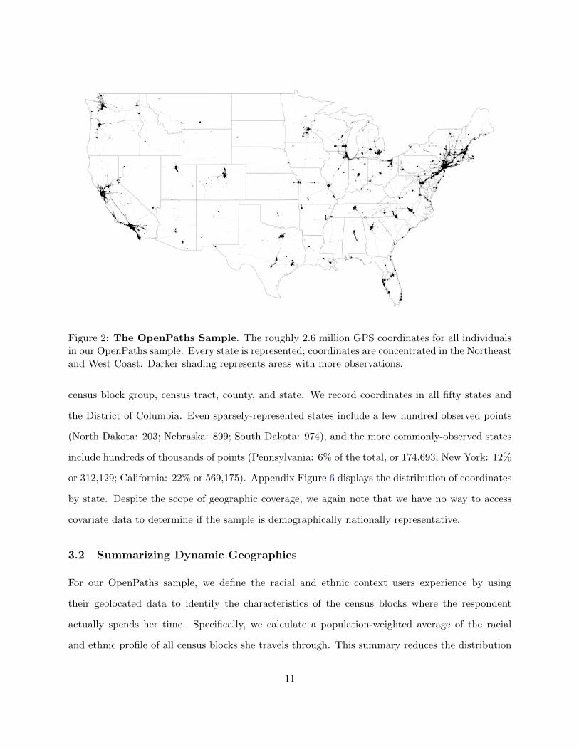
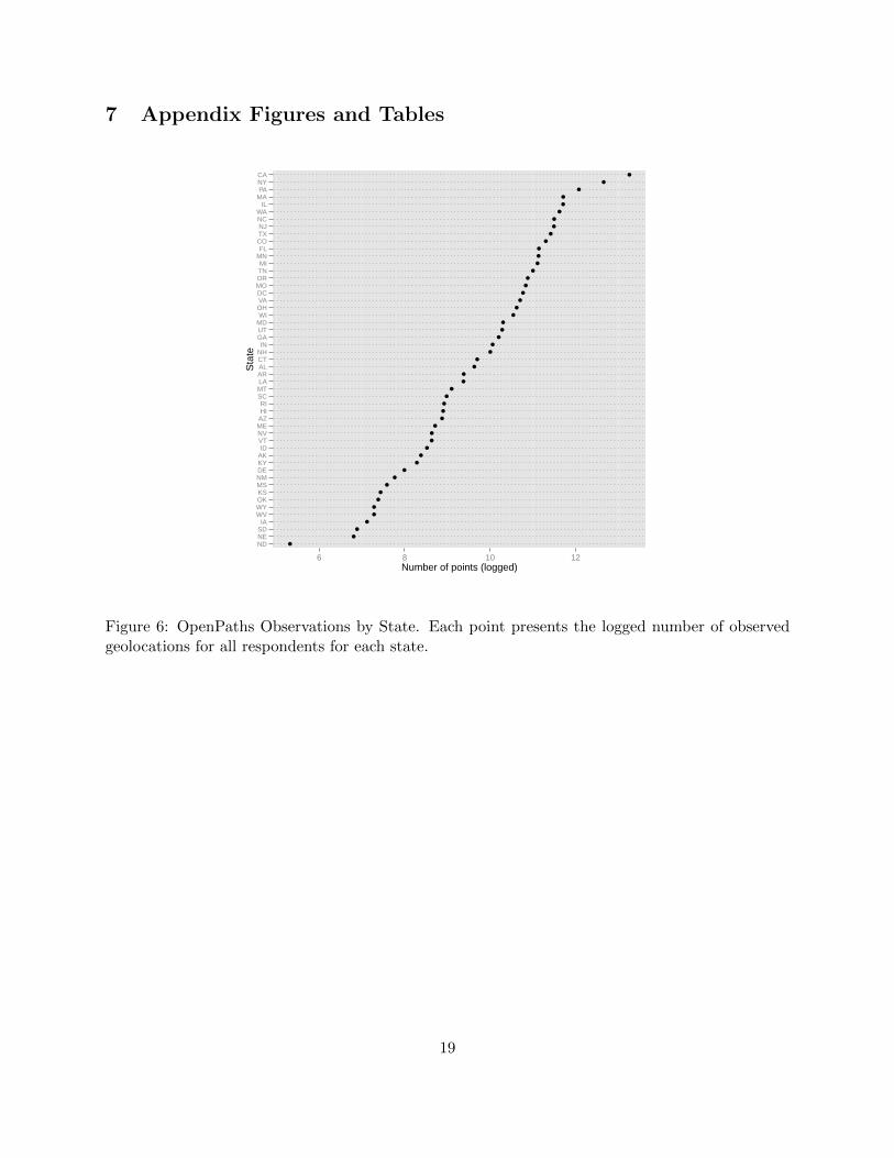
Figure 2: The OpenPaths Sample. The roughly 2.6 million GPS coordinates for all individualsin our OpenPaths sample. Every state is represented; coordinates are concentrated in the Northeastand West Coast. Darker shading represents areas with more observations.
census block group, census tract, county, and state. We record coordinates in all fifty states and
the District of Columbia. Even sparsely-represented states include a few hundred observed points
(North Dakota: 203; Nebraska: 899; South Dakota: 974), and the more commonly-observed states
include hundreds of thousands of points (Pennsylvania: 6% of the total, or 174,693; New York: 12%
or 312,129; California: 22% or 569,175). Appendix Figure 6 displays the distribution of coordinates
by state. Despite the scope of geographic coverage, we again note that we have no way to access
covariate data to determine if the sample is demographically nationally representative.
3.2 Summarizing Dynamic Geographies
For our OpenPaths sample, we define the racial and ethnic context users experience by using
their geolocated data to identify the characteristics of the census blocks where the respondent
actually spends her time. Specifically, we calculate a population-weighted average of the racial
and ethnic profile of all census blocks she travels through. This summary reduces the distribution
11
of characteristics in the visited blocks to a single measure of context. This measure is a useful
summary; as we show below, however, we can leverage a great deal more information about the
distribution of blocks each individual experiences.
4 How Static Measures Fail to Capture Dynamic Contexts
We compare our dynamic measure of context to a wide variety of static measures, representing a
range of approaches scholars have adopted in describing racial and ethnic context. In doing so,
we arrive at two core conclusions. First, static measures are poor proxies for individuals’ dynamic
experiences. This mismeasurement persists even at the census block level, the lowest geography for
which data are available. Second, low levels of static geography can be used to estimate dynamic
experiences, but not uniformly across racial and ethnic groups.
4.1 Describing the Mismeasurement
For each OpenPaths participant, we designate modal geographies. These geographies, in which
the participant appears most, represent our estimates of the geographic containers (block, block
group, tract, county, and state) into which a survey researcher measuring context would place
the respondent. These geographies serve as static measures that we compare to the participant’s
dynamic context. To summarize the dynamic context, we take the mean percentage of residents of a
given race in the census blocks through which the participant travels, weighted by block population.
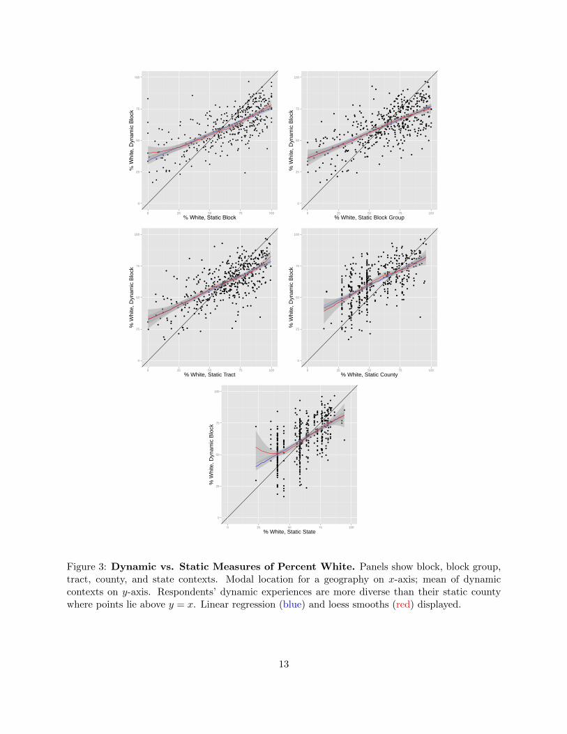
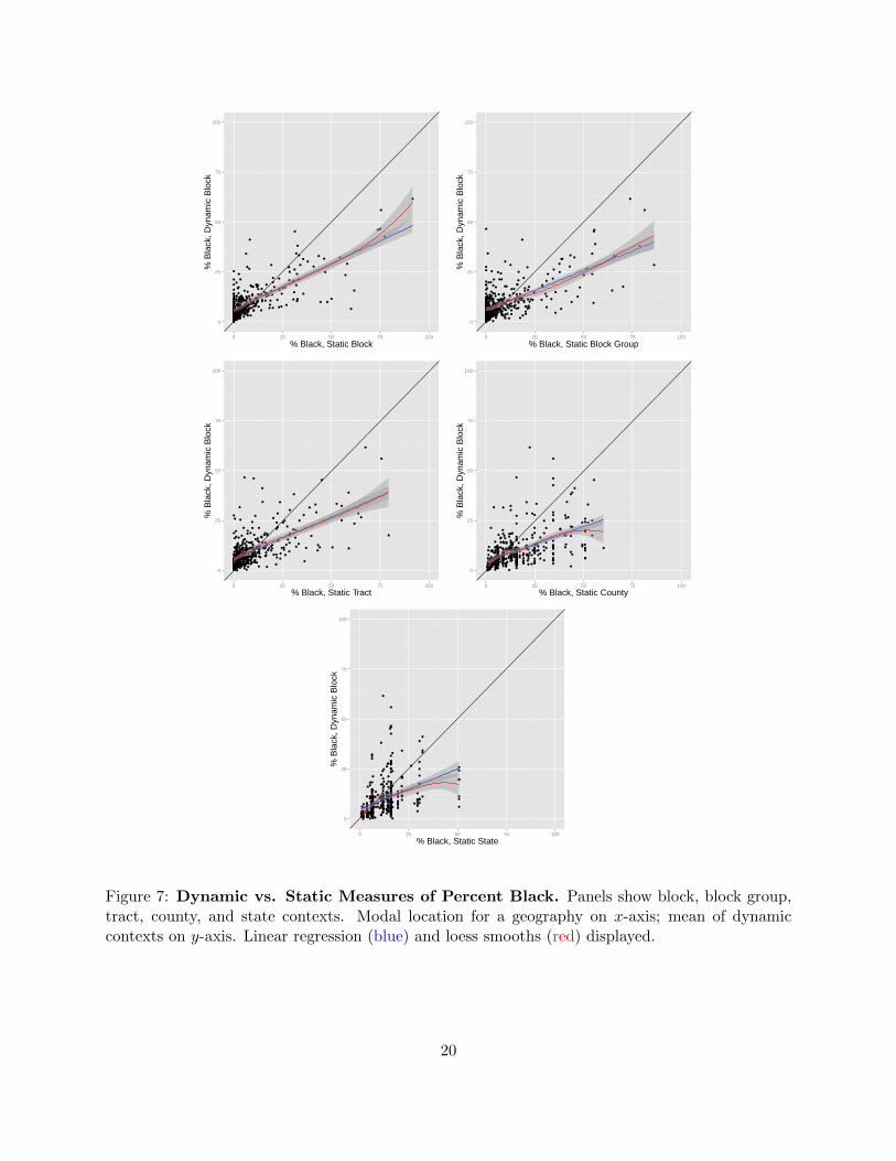
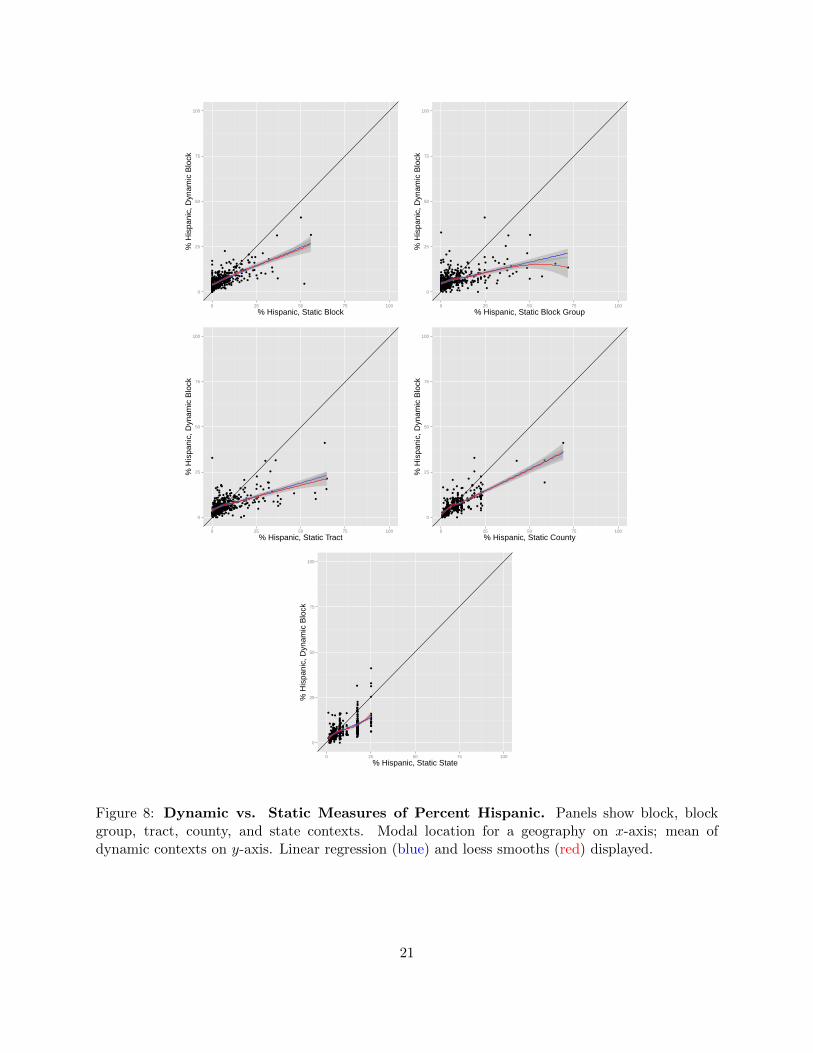
Figure 3 and supplementary Figures 7 through 9 plot our dynamic measure of racial and ethnic
context on the y-axis against a static measure on the x-axis. Each figure compares measures for
one racial or ethnic group, and each panel compares the dynamic measure to a different level of
geography. If static measures of geography were perfect proxies for respondents’ experiences, then
every point would lie on the black y = x line in each panel. Clearly, this is not the case, and
there are important systematic differences between the two measures. Where points fall above the
y = x line, the static measure understates the individual’s experience with members of that racial
or ethnic group; where they fall below, the static measure overstates their experience.
First, individual experiences of racial and ethnic context are typically more moderate than
12
●
● ●
●
●
●
●
●
●
●
●
●
●
●
●
●
●
●
●
●
●
●
●
●
●
●
●
●
●
●
●
●
●
●
●
●●
●
●
●
●
●
●
●
●
●
●
●
●
●
●
●
●
●
●
●
●
●
●
●
●
●
●
●
● ●
●
●
●
●
●
●
●
●
●
●
●
●
●
●
●
●
●
●●
●
●
●
●
●
●
●
●
●
●
●
●●
●
●
●
●
●
●
●
●
●
●
●
●
●
●
●
●
●●
●
●
●
●
●
●
●
●
●
●
●●
●
●
●●
●
●
●
●
●
●
●
●
●
●
●
●
●
●
●
●
●
●
●
●
●
●
●
●
●
●
●
●
●
●
●
●●
●
●
●
●
●
●
● ●
●
●
●
●
●●
●
●
●
●
●
●
●
●
●
●
●
●
●
●●
●
●
●
●
●●
●
●
●
●
●
●
●
● ●
●
●
●
● ●
●
●
●
●
●
●
●
●
●
●
●
●
●
●
●
●
●
●
●
●
●
●
●
●
●
●
●
●
●
●
●
●
●
●
●
●
●
●
●
●●
●
●
●
●
●
●
●
●
●
●
●
●
●
●
●●
●●
●
●
●
●
●
●
●
●
●
●
●
●
●
●
● ●
●
●
●
●
●
●
●
●
●
●●
●
●
●
●
●
●
●
●
●
●
●
●
●
●
●
●
●
●
●
●
●
●
●
●
●
●
●
●
●
●
●
●
●
●
●
●
●
●
●
●
●
●
●
●
●
●
●
●
●
●
●
●
●
●
●
●
●
●
●
●
●
●
●
●
●
●
●
●●
●
●
●
●
●
●
●
●
●
●
●
●
●
●
●
●
●
●
0
25
50
75
100
0 25 50 75 100% White, Static Block
% W
hite
, Dyn
amic
Blo
ck
●
● ●
●
●
●
●
●
●
●
●
●
●
●
●
●
●
●
●
●
●
●
●
●
●
●
●
●
●
●
●
●
●
●
●
●
●●
●
●
●
●
●
●
●
●
●
●
●
●
●
●
●
●
●
●
●
●
●
●
●
●
●
●●
●
●
●
● ●
●
●
●
●
●
●
●
●
●
●
●
●
●
●
●
●
●
●
●●
●● ●
●
●
●
●
●
●
●
●
●
●
●
●
●
●
●
●
●
●
●
●
●
●
●
●
●
●
●
●
●
●
●
●●
●
●
●
●
●
●
●
●
●
●
●●
●
●
●
●
●
●
●
●
●
●
●
●
●
●
●
●
●
●
●
●
●
●
●
●
●
●
●
●
●●
●
●
●
●
●
●
●
●
●
●
●●
●
●
●
●
●
●
●
● ●
●
●
●
●
●●
●
●
●
●
●
●
●
●
●
●
●
●
●●
●
●
●
●
●
●
●●
●
●
●
●
●
●
●
● ●
●
●
●
●●
●
●
●
●
●
●
●
●
●
●
●
●
●
●
●
●
●
●
●
●
●
●
●
●
●
●
●
●
●
●
●
●
●
●
●
●
●
●
●●
●
●
●
●
●
●
●●
●
●
●
●
●
●
● ●
●
●
●
●
●
●
●
●
●
●
●
●
●●
●●
●
●
●
●
●
●
●
●
●
●
●
●
●
●
●
●
●
●
●
●
●
●
●
●
●
●
●
●
●
●●
●
●
●
●
●
●
●
●
●
●
●
●
●
●
●
●
●
●
●
●
●
●
●
●
●
●
●
●
●
●
●
●
●
●
●
●
●
●
●
●
●
●
●
●
●
●
●
●
●
●
●
●
●
●
●
●
●
●
●
●
●
●
●
●
●
●
●
●
●
●
●
●
●
●
●●
●
●●
●
●
●
●
●
●
●
●
●
●
●
●
●
●
●
●
●
●
●
●
●
0
25
50
75
100
0 25 50 75 100
% White, Static Block Group
% W
hite
, Dyn
amic
Blo
ck
●
● ●
●
●
●
●
●
●
●
●
●
●
●
●
●
●
●
●
●
●
●
●
●
●
●
●
●
●
●
●
●
●
●
●
●
●
●●
●
●
●
●
●
●
●
●
●
●
●
●
●
●
●
●
●
●
●
●
●
●
●
●
●
●●
●
●
●
● ●
●
●
●
●
●
●
●
●
●
●
●
●
●
●
●
●
●
●
●●
●● ●
●
●
●
●
●
●
●
●
●
●
●
●
●
●
●
●
●
●
●
●
●
●
●
●
●
●
●
●
●
●
●
●
●●
●
●
●
●
●
●
●
●
●
●
●●
●
●
●
●
●
●
●
●
●
●
●
●
●
●
●
●
●
●
●
●
●
●
●
●
●
●
●
●
●●
●
●
●
●
●
●
●
●
●
●
●
●●
●
●
●
●
●
●
●
●●
●
●
●
●
●●
●
●
●
●
●
●
●
●
●
●
●
●
●
●●
●
●
●
●
●
●
●●
●
●
●
●
●
●
●
● ●
●
●
●
● ●
●
●
●
●
●
●
●
●
●
●
●
●
●
●
●
●
●
●
●
●
●
●
●
●
●
●
●
●
●
●
●
●
●
●
●
●
●
●
●
●●
●
●
●
●
●
●
●●
●
●
●
●
●
●
● ●
●
●
●
●
●
●
●
●
●
●
●
●
●●
●●
●
●
●
●
●
●
●
●
●
●
●
●
●
●
●
●
●
●
●
●
●
●
●
●
●
●
●
●
●
●●
●
●
●
●
●
●
●
●
●
●
●
●
●
●
●
●
●
●
●
●
●
●
●
●
●
●
●
●
●
●
●
●
●
●
●
●
●
●
●
●
●
●
●
●
●
●
●
●
●
●
●
●
●
●
●
●
●
●
●
●
●
●
●
●
●
●
●
●
●
●
●
●
●
●
●●
●
●●
●
●
●
●
●
●
●
●
●
●
●
●
●
●
●
●
●
●
●
●
●
0
25
50
75
100
0 25 50 75 100
% White, Static Tract
% W
hite
, Dyn
amic
Blo
ck
●
● ●
●
●
●
●
●
●
●
●
●
●
●
●
●
●
●
●
●
●
●
●
●
●
●
●
●
●
●
●
●
●
●
●
●
●
● ●
●
●
●
●
●
●
●
●
●
●
●
●
●
●
●
●
●
●
●
●
●
●
●
●
●
●●
●
●
●
●●
●
●
●
●
●
●
●
●
●
●
●
●
●
●
●
●
●
●
●
●
●
●
●● ●
●
●
●
●
●
●
●
●
●
●
●
●
●
●
●
●
●
●
●
●
●
●
●
●
●
●
●
●
●
●
●
●
●●
●
●
●
●
●
●
●
●
●
●
●●
●
●
●
●
●
●
●
●
●
●
●
●
●
●
●
●
●
●
●
●
●
●
●
●
●
●
●
●
●●
●
●
●
●
●
●
●
●
●
●
●
●●
●
●
●
●
●
●
●
●●
●
●
●
●
●●
●
●
●
●
●
●
●
●
●
●
●
●
●
●
●●
●
●
●
●
●
●
●●
●
●
●
●
●
●
●
●●
●
●
●
● ●
●
●
●
●
●
●
●
●
●
●
●
●
●
●
●
●
●
●
●
●
●
●
●
●
●
●
●
●
●
●
●
●
●
●
●
●
●
●
●
●●
●
●
●
●
●
●
●●
●
●
●
●
●
●
● ●
●
●
●
●
●
●
●
●
●
●
●
●
●●
●●
●
●
●
●
●
●
●
●
●
●
●
●
●
●
●
●
●
●
●
●
●
●
●
●
●
●
●
●
●
●●
●
●
●
●
●
●
●
●
●
●
●
●
●
●
●
●
●
●
●
●
●
●
●
●
●
●
●
●
●
●
●
●
●
●
●
●
●
●
●
●
●
●
●
●
●
●
●
●
●
●
●
●
●
●
●
●
●
●
●
●
●
●
●
●
●
●
●
●
●
●
●
●
●
●
●
●●
●
● ●
●
●
●
●
●
●
●
●
●
●
●
●
●
●
●
●
●
●
●
●
●
●
0
25
50
75
100
0 25 50 75 100
% White, Static County
% W
hite
, Dyn
amic
Blo
ck
●
● ●
●
●
●
●
●
●
●
●
●
●
●
●
●
●
●
●
●
●
●
●
●
●
●
●
●
●
●
●
●
●
●
●
●
●
● ●
●
●
●
●
●
●
●
●
●
●
●
●
●
●
●
●
●
●
●
●
●
●
●
●
●
●●
●
●
●
●●
●
●
●
●
●
●
●
●
●
●
●
●
●
●
●
●
●
●
●
●
●
●
●● ●
●
●
●
●
●
●
●
●
●
●
●
●
●
●
●
●
●
●
●
●
●
●
●
●
●
●
●
●
●
●
●
●
●●
●
●
●
●
●
●
●
●
●
●
●●
●
●
●
●
●
●
●
●
●
●
●
●
●
●
●
●
●
●
●
●
●
●
●
●
●
●
●
●
●●
●
●
●
●
●
●
●
●
●
●
●
●●
●
●
●
●
●
●
●
●●
●
●
●
●
●●
●
●
●
●
●
●
●
●
●
●
●
●
●
●
●●
●
●
●
●
●
●
●●
●
●
●
●
●
●
●
●●
●
●
●
●●
●
●
●
●
●
●
●
●
●
●
●
●
●
●
●
●
●
●
●
●
●
●
●
●
●
●
●
●
●
●
●
●
●
●
●
●
●
●
●
●●
●
●
●
●
●
●
●●
●
●
●
●
●
●
● ●
●
●
●
●
●
●
●
●
●
●
●
●
●●
● ●
●
●
●
●
●
●
●
●
●
●
●
●
●
●
●
●
●
●
●
●
●
●
●
●
●
●
●
●
●
●●
●
●
●
●
●
●
●
●
●
●
●
●
●
●
●
●
●
●
●
●
●
●
●
●
●
●
●
●
●
●
●
●
●
●
●
●
●
●
●
●
●
●
●
●
●
●
●
●
●
●
●
●
●
●
●
●
●
●
●
●
●
●
●
●
●
●
●
●
●
●
●
●
●
●
●
●●
●
● ●
●
●
●
●
●
●
●
●
●
●
●
●
●
●
●
●
●
●
●
●
●
●
0
25
50
75
100
0 25 50 75 100
% White, Static State
% W
hite
, Dyn
amic
Blo
ck
Figure 3: Dynamic vs. Static Measures of Percent White. Panels show block, block group,tract, county, and state contexts. Modal location for a geography on x-axis; mean of dynamiccontexts on y-axis. Respondents’ dynamic experiences are more diverse than their static countywhere points lie above y = x. Linear regression (blue) and loess smooths (red) displayed.
13
static measures suggest. When a respondent’s modal census block has a small percentage of a
given racial or ethnic group, static representation understates how much the individual experiences
members of that race or ethnicity. At the extreme, for example, for participants’ whose modal
block is 0% white (those at the very left-hand side of the first panel in Figure 3), the static measure
underestimates their average experience of whites, who actually comprise between 25 and about
80% of the census blocks these participants experience.10 The y-intercept of the bivariate linear
regression line gives a sense of the average “bias” in the static measure at this point–about 34
percentage points (Tufte, 1973). At the other extreme, static blocks that are majority white tend
to overrepresent participants’ average experience of whites; most points at the right side of the
panel fall below the y = x line.
Second, it does not appear that the dynamic measure is simply the static measure “regressed
to the mean.” Comparing our dynamic block-level milieu to the typical static county measure, for
example, over two-thirds of the sample has its dynamic diversity understated by the static measure.
Third, the comparison of dynamic to static measures at the same low level of geography (the
census block) demonstrates that the mismeasurement of geographic context is not merely a problem
caused by high levels of aggregation, but also a failure to account for how individuals travel through
their environments. We observe the same pattern across racial and ethnic groups and geographies,
though with a few exceptions. As the last panel of Appendix Figure 9 shows, for example, static
state measures nearly always underestimate the percentage of Asians in the blocks participants
travel through.
The intercept of each regression line indicates the bias in static measures for those whose modal
location for a given geography lacks members of a particular race or ethnicity. The slopes provide
guidance for how to translate from static measures to dynamic ones. For example, the slope in the
first panel of Figure 3 is 0.4, indicating that on average, an individual from a block 10 percentage
points more white than another actually only experiences about 4 percentage points more whites.
We provide coefficient estimates for the full set of linear models in Appendix Table 2.
10We follow the convention of using “white” to mean white, non-Hispanic or -Latino. “Non-whites” include His-panics, Latinos, and those giving non-white racial identities.
14
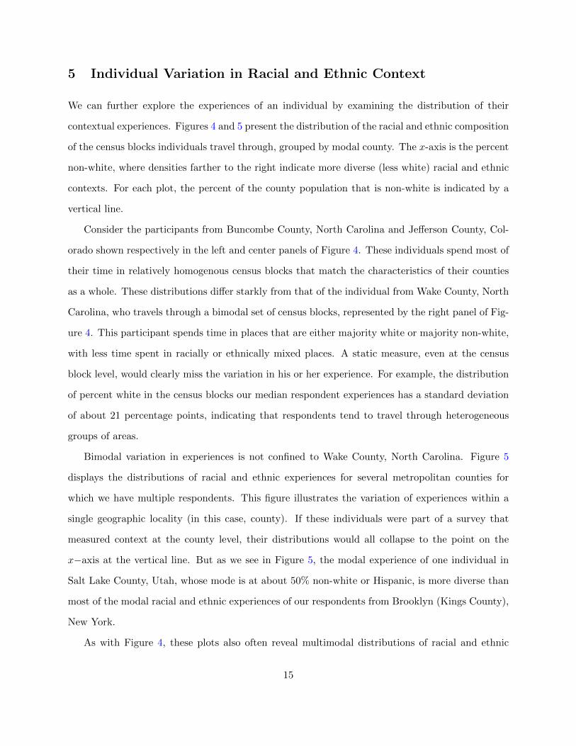
5 Individual Variation in Racial and Ethnic Context
We can further explore the experiences of an individual by examining the distribution of their
contextual experiences. Figures 4 and 5 present the distribution of the racial and ethnic composition
of the census blocks individuals travel through, grouped by modal county. The x-axis is the percent
non-white, where densities farther to the right indicate more diverse (less white) racial and ethnic
contexts. For each plot, the percent of the county population that is non-white is indicated by a
vertical line.
Consider the participants from Buncombe County, North Carolina and Jefferson County, Col-
orado shown respectively in the left and center panels of Figure 4. These individuals spend most of
their time in relatively homogenous census blocks that match the characteristics of their counties
as a whole. These distributions differ starkly from that of the individual from Wake County, North
Carolina, who travels through a bimodal set of census blocks, represented by the right panel of Fig-
ure 4. This participant spends time in places that are either majority white or majority non-white,
with less time spent in racially or ethnically mixed places. A static measure, even at the census
block level, would clearly miss the variation in his or her experience. For example, the distribution
of percent white in the census blocks our median respondent experiences has a standard deviation
of about 21 percentage points, indicating that respondents tend to travel through heterogeneous
groups of areas.
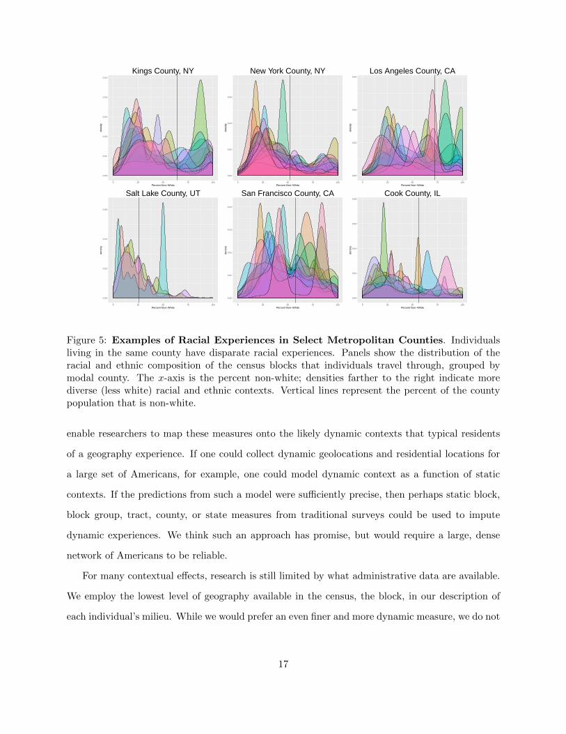
Bimodal variation in experiences is not confined to Wake County, North Carolina. Figure 5
displays the distributions of racial and ethnic experiences for several metropolitan counties for
which we have multiple respondents. This figure illustrates the variation of experiences within a
single geographic locality (in this case, county). If these individuals were part of a survey that
measured context at the county level, their distributions would all collapse to the point on the
x−axis at the vertical line. But as we see in Figure 5, the modal experience of one individual in
Salt Lake County, Utah, whose mode is at about 50% non-white or Hispanic, is more diverse than
most of the modal racial and ethnic experiences of our respondents from Brooklyn (Kings County),
New York.
As with Figure 4, these plots also often reveal multimodal distributions of racial and ethnic
15
0.00
0.01
0.02
0.03
0.04
0 25 50 75 100Percent Non−White
dens
ityBuncombe County, NC
0.00
0.05
0.10
0 25 50 75 100Percent Non−White
dens
ity
Jefferson County, CO
0.00
0.02
0.04
0 25 50 75 100Percent Non−White
dens
ity
Wake County, NC
Figure 4: Racial Experiences that are Unimodal and Bimodal. For some individuals,county captures both the mean and modal experience of the individual (left and center panels).For others (right panel), the county obscures the distribution of racial experiences. Panels show thedistributions of racial and ethnic composition of the census blocks that individuals travel through,grouped by modal county. The x-axis is the percent non-white; densities farther to the rightindicate more diverse (less white) racial and ethnic contexts. Vertical lines represent the percentof the county population that is non-white.
experiences. We provide an example of a multimodal census block distribution within a county
elsewhere, showing that even if an individual experienced every census block in her county, the
summary measure could still mask extreme experiences (Moore and Reeves, 2017). How might the
attitudes of someone who spends their time in one type of census blocks vary from those of an
individual who travels from one contextual extreme to another, even if their average experiences
are the same? Subsequent stages of this research will pair geolocation data with survey responses,
allowing scholars to move beyond questions about population levels in static geographic containers
to questions that consider the full distribution of dynamic contextual experiences.
6 Discussion
We demonstrate that static measures of lived experience, usually defined by residence at a single
level of geography, fail to capture the variety of experiences that individuals are often posited to
have. In some cases, these systematic misrepresentations represent a form of measurement error
that plagues estimates of the effects of racial and ethnic context (e.g., Cho and Baer, 2011).
Where scholars only have access to traditional measures of context, future modeling efforts may
16
0.00
0.01
0.02
0.03
0.04
0.05
0 25 50 75 100Percent Non−White
dens
ity
Kings County, NY
0.00
0.02
0.04
0.06
0 25 50 75 100Percent Non−White
dens
ity
New York County, NY
0.00
0.02
0.04
0.06
0 25 50 75 100Percent Non−White
dens
ity
Los Angeles County, CA
0.00
0.02
0.04
0.06
0 25 50 75 100Percent Non−White
dens
ity
Salt Lake County, UT
0.00
0.01
0.02
0.03
0.04
0 25 50 75 100Percent Non−White
dens
ity
San Francisco County, CA
0.00
0.02
0.04
0.06
0.08
0 25 50 75 100Percent Non−White
dens
ity
Cook County, IL
Figure 5: Examples of Racial Experiences in Select Metropolitan Counties. Individualsliving in the same county have disparate racial experiences. Panels show the distribution of theracial and ethnic composition of the census blocks that individuals travel through, grouped bymodal county. The x-axis is the percent non-white; densities farther to the right indicate morediverse (less white) racial and ethnic contexts. Vertical lines represent the percent of the countypopulation that is non-white.
enable researchers to map these measures onto the likely dynamic contexts that typical residents
of a geography experience. If one could collect dynamic geolocations and residential locations for
a large set of Americans, for example, one could model dynamic context as a function of static
contexts. If the predictions from such a model were sufficiently precise, then perhaps static block,
block group, tract, county, or state measures from traditional surveys could be used to impute
dynamic experiences. We think such an approach has promise, but would require a large, dense
network of Americans to be reliable.
For many contextual effects, research is still limited by what administrative data are available.
We employ the lowest level of geography available in the census, the block, in our description of
each individual’s milieu. While we would prefer an even finer and more dynamic measure, we do not
17
yet have, for example, a measure of the people within a participant’s field of vision. Currently, we
are limited to the characteristics of a milieu that are collected at that administrative level. Despite
this limitation, we argue that the dynamic collection of relatively small administrative contexts
approximates the actual environment one experiences better than current practices. In the future,
we could develop additional dynamic measures by defining age contexts, for example, using block
level data. Any time researchers have geographic data, dynamic contexts could be defined using
the variables available for that container.
Our data collection strategy reflects larger trends toward exploiting geographic social scientific
data. Significant geolocation efforts stand to revolutionize the study of disease patterns, for exam-
ple, and the study of racial and ethnic contextual effects should follow. Scholars have long been
interested in the effects of milieus on a variety of outcomes. However, only recently has the ability
to precisely, dynamically measure where individuals travel in their daily lives become affordable
and unintrusive enough to be feasible for large social scientific samples. With the ability to collect
frequent individual geolocations, political science can better link empirical measures to theoretical
concepts like racial and ethnic milieus.
18
7 Appendix Figures and Tables
●
●
●
●
●
●
●
●
●
●
●
●
●
●
●
●
●
●
●
●
●
●
●
●
●
●
●
●
●
●
●
●
●
●
●
●
●
●
●
●
●
●
●
●
●
●
●
●
●
●
●NDNESDIA
WVWYOKKSMSNMDEKYAKIDVTNVMEAZHIRI
SCMTLAARALCTNHIN
GAUTMDWI
OHVADCMOORTNMI
MNFL
COTXNJNCWA
ILMAPANYCA
6 8 10 12Number of points (logged)
Sta
te
Figure 6: OpenPaths Observations by State. Each point presents the logged number of observedgeolocations for all respondents for each state.
19
●
●
●●
●
●
●
●
●
●
●●
●
●
●
●
●●
●
●
●
●
●
●
●●
●
●
●
●
●
●
●
●
●
●
●
●
●
●
●
●●
●
●
●
●
● ●●
●
●●
●
●
●
●
●
●●
●
●
●
●
●
●
●
●
● ●
●
●
●
●
●
●
●
●
●
●
●
●
●
●
●
●
●
●
●
●
●
●●
●
●
●
●●
●
●
●●
●
●
●
●
●
●
●●
●
●●
●●●●
●●
●
●
●
●
●
●
●
●●
●
●
●
●
●
●
●
●
●
●
●●
●
●
●
●
●
●
●
●●
●
●
●
●●●
●●●
●
●
●
●
●
● ●
●
●
●●●
●
●●
●●
●●●
●●
●
●
●
●
●
●
●
●
●
●
● ●
●
●
●
●
●
●
●
●
●
●
●
●
●
●
●
●
●
●
●
●
●
●
●
●
●
●
● ●
● ●
●
●
●
●
●
●
●
●
●
●
●
●
●●●
● ●
●
●
●●
●
●
●
●
●
●
●
●
●
●
●
●
●
●
●
●
●
●
●
●
●
●
●
●
●
●
●
●
●
●
●
●
●
●
●●
●
●●
●
●
●
●
●
●
●
●
●
●
●
●
●
●
●
●
●
●
●
●●
●
●
●
●
●
●
●●
● ● ●●
●
●
●
●
●
●
●
●
●
●
●
●
●
●
●
●
●
●
●
●●
●
●
●
●
●
● ●
●
●
●
●●
● ●●
●
●
●
●
●●●
●
●
●
●
●
●●
●
●
●
●
●
●
●
●●
●
●
●
●
●
●●
●
●
●●
●●
0
25
50
75
100
0 25 50 75 100
% Black, Static Block
% B
lack
, Dyn
amic
Blo
ck
●
●
●●
●
●
●
●
●
●
●●
●
●
●
●
●●
●
●
●
●
●
●
●
●
●
●
●
●
●
●
●
●
●
●
●
●
●
●
●
●
●
●●
●
●
●
●
● ●●
●
● ●
●
●
●
●
●
●
●●
●●
●
●
●
●
●
●
●
●●
●
●
●
●
●
●
●
●
●
●
●
●
●
●
●
●
●
●
●
●●
●
●
●
●
●●
●
●
●
●
●
●
●
●●
●
●
●
●
●
●
●
●
● ●
●
●●
●●●●
● ●
●
●
●
●
●
●
●
●●
●
●
●
●
●
●
●
●
●
●
●
●
●●
●
●
●
●
●
●
●
●●
●
●
●
●●
●
●
●
●● ●
●
●
●
●
●
●
● ●
●
●
●●
●
●
●
●●
●●
●●●
●●
●
●
●
●
●
●
●
●
●●●
●
●
●
●
●
●
●●
●
●
●
●
●
●
●
●
●
●
●
●
●
●
●
●
●
●
●
●
●
●●
●●
●●
●
●
●
●
●
●
●
●
●
●
●● ●
● ●●
●
●
●
●●
●
●● ●
●
●
●●
●
●
●
●
●
●
●
●
●
●
●
●
●
●●
●
●
●
●
●
●
●
●●
●
●
●
●
●
●
●
●
●
●
●
●
●●
●
●●
●
●
●
●
●
●
●
●
●
●
●
●
●
●
●
●
●
●
●
●
●
●
●
●
●●
●
●
●
●
●
●
●●
● ●●
●
●
●
●
●
●
●
●
●
●
●
●
●
●
●
●
●
●
●
●
●
●
●
●
●●
●
●
●
●
●
●
● ●
●
●
●
●●
●●●●
●
●
●
●●●
●
●
●
●
●
●●
●
●
●
●
●
●
●
●
●
●
●●
●●
●
●
●
●
●
●●●
●
●
●●
●
●
●
0
25
50
75
100
0 25 50 75 100
% Black, Static Block Group
% B
lack
, Dyn
amic
Blo
ck
●
●
●●
●
●
●
●
●
●
●●
●
●
●
●
●●
●
●
●
●
●
●
●
●●
●
●
●
●
●
●
●
●
●
●
●
●
●
●
●
●
●
●●
●
●
●
●
●●●
●
●●
●
●
●
●
●
●
●●
●●
●
●
●
●
●
●
●
●●
●
●
●
●
●
●
●
●
●
●
●
●
●
●
●
●
●
●
●
●●
●
●
●
●
●●
●
●
●
●
●
●
●
●
●●
●
●
●
●
●
●
●
●
● ●
●
●●
●●●●
● ●
●
●
●
●
●
●
●
●●●
●
●
●
●
●
●
●
●
●
●
●
●●
●
●
●
●
●
●
●
●●
●
●
●
●●
●
●
●
●
●● ●
●
●
●
●
●
●
● ●
●
●
●●
●
●
●
●●
●●
●●●
●●
●
●
●
●
●
●
●
●
●
●● ●
●
●
●
●
●
●
●●
●
●
●
●
●
●
●
●
●
●
●
●
●
●
●
●
●
●
●
●
●
● ●
●●
●●
●
●
●
●
●
●
●
●
●
●
●
●● ●
● ●●
●
●
●
●●
●
●●●
●
●
●●
●
●
●
●
●
●
●
●
●
●
●
●
●
●●
●
●
●
●
●
●
●
● ●
●
●
●
●
●
●
●
●
●
●
●
●
●●
●
●●
●
●
●
●
●
●
●
●
●
●
●
●
●
●
●
●
●
●
●
●
●
●
●
●
●●
●
●
●
●
●
●
●●
● ●●
●
●
●
●
●
●
●
●
●
●
●
●
●
●
●
●
●
●
●
●
●
●
●
●
●●
●
●
●
●
●
●
●●
●
●
●
●●
●●●
●
●
●
●
●● ●
●
●
●
●
●
●●
●
●
●
●
●
●
●
●
●
●
●●
●●
●
●
●
●
●
●●●
●
●
●●
●
●
●
0
25
50
75
100
0 25 50 75 100
% Black, Static Tract
% B
lack
, Dyn
amic
Blo
ck
●
●
●●
●
●
●
●
●
●
●●
●
●
●
●
●●
●
●
●
●
●
●
●
●●
●
●
●
●
●
●
●
●
●
●
●
●
●
●
●
●
●
●●
●
●
●
●
●●●
●
●●
●
●
●
●
●
●
●●
●●
●
●
●
●
●
●
●
● ●
●
●
●
●
●
●
●
●
●
●
●
●
●
●
●
●
●●
●
●
●
●●
●
●
●
●
●●
●
●
●
●
●
●
●
●
●●
●
●
●
●
●
●
●
●
●●
●
●●
●●
●●
●●
●
●
●
●
●
●
●
●●
●
●
●
●
●
●
●
●
●
●
●
●
●●
●
●
●
●
●
●
●
●●
●
●
●
●●
●
●
●
●
●● ●
●
●
●
●
●
●
●●
●
●
●●
●
●
●
●●
●●
●●●
●●
●
●
●
●
●
●
●
●
●
●
●
●●
●
●
●
●
●
●
●●
●
●
●
●
●
●
●
●
●
●
●
●
●
●
●
●
●
●
●
●
●
● ●
● ●
●●
●
●
●
●
●
●
●
●
●
●
●
●● ●
●●●
●
●
●
●●
●
●● ●
●
●
●●
●
●
●
●
●
●
●
●
●
●
●
●
●
●●
●
●
●
●
●
●
●
● ●
●
●
●
●
●
●
●
●
●
●
●
●
● ●
●
●●
●
●
●
●
●
●
●
●
●
●
●
●
●
●
●
●
●
●
●
●
●
●
●
●
●●
●
●
●
●
●
●
●●
● ●●
●
●
●
●
●
●
●
●
●
●
●
●
●
●
●
●
●
●
●
●
●
●
●
●
●
●●
●
●
●
●
●
●
●●
●
●
●
●●
●●●
●
●
●
●
●● ●
●
●
●
●
●
●●
●
●
●
●
●
●
●
●
●
●
●●
●●
●
●
●
●
●
●
●
● ●
●
●
●●
●
●
●
0
25
50
75
100
0 25 50 75 100
% Black, Static County
% B
lack
, Dyn
amic
Blo
ck
●
●
●●
●
●
●
●
●
●
●●
●
●
●
●
●●
●
●
●
●
●
●
●
●●
●
●
●
●
●
●
●
●
●
●
●
●
●
●
●
●
●
●●
●
●
●
●
●●●
●
●●
●
●
●
●
●
●
●●
●●
●
●
●
●
●
●
●
● ●
●
●
●
●
●
●
●
●
●
●
●
●
●
●
●
●
●●
●
●
●
●●
●
●
●
●
●●
●
●
●
●
●
●
●
●
●●
●
●
●
●
●
●
●
●
●●
●
●●
●●
●●
●●
●
●
●
●
●
●
●
●●
●
●
●
●
●
●
●
●
●
●
●
●
●●
●
●
●
●
●
●
●
●●
●
●
●
●●
●
●
●
●
●●●
●
●
●
●
●
●
● ●
●
●
●●
●
●
●
●●
●●
●●●
●●
●
●
●
●
●
●
●
●
●
●
●
● ●
●
●
●
●
●
●
●●
●
●
●
●
●
●
●
●
●
●
●
●
●
●
●
●
●
●
●
●
●
● ●
●●
●●
●
●
●
●
●
●
●
●
●
●
●
●● ●
●●●
●
●
●
●●
●
●● ●
●
●
●●
●
●
●
●
●
●
●
●
●
●
●
●
●
●●
●
●
●
●
●
●
●
● ●
●
●
●
●
●
●
●
●
●
●
●
●
●●
●
●●
●
●
●
●
●
●
●
●
●
●
●
●
●
●
●
●
●
●
●
●
●
●
●
●
●●
●
●
●
●
●
●
●●
● ● ●
●
●
●
●
●
●
●
●
●
●
●
●
●
●
●
●
●
●
●
●
●
●
●
●
●
●●
●
●
●
●
●
●
●●
●
●
●
●●
●●●●
●
●
●
●●●
●
●
●
●
●
●●
●
●
●
●
●
●
●
●
●
●
●●
●●
●
●
●
●
●
●
●
● ●
●
●
●●
●
●
●
0
25
50
75
100
0 25 50 75 100
% Black, Static State
% B
lack
, Dyn
amic
Blo
ck
Figure 7: Dynamic vs. Static Measures of Percent Black. Panels show block, block group,tract, county, and state contexts. Modal location for a geography on x-axis; mean of dynamiccontexts on y-axis. Linear regression (blue) and loess smooths (red) displayed.
20
●●●
●
●
●
●
●●
●
●
●●●
●
●●
●●
●
●●
●
●
●●
●
●
●●
●
●
●
●
●
●
●
●
● ●
●
●
●●
●
●
●
●
●
●
●
●
●
●
●
●
●●
●
●
●
●
●
●
●
●
●
●●●
●●
●
●
●
●●●
●●
●
●
●
●
●
●
●
●
●●
●
●
●
●
●
●
●
●
●
●●
●●
●
●
●
●
●
●
●●
●
●
●
●
●●●
●
●
●●
●
●
●
●
●
●●
●●
●
●
●●
●
●
●
●
●
●
●
●
●●
●
●●
●
●
●
●
●●●
●
●●
●
●
●
●●
●
●
●
●
●
●
●
●
●
●
●●
●
●
●
●
●●
●●
●
●●
●●●
●
●
●
●
●●
●
●●
●
● ●
●
●●
●
●
●
●●
●
●
●
●●
●
●
●●●
●
●●
●
●
●●
●
●●
●●
●
●
●
●● ●●
●
●●
●
●
●
●
●
●
●
●
●
●
●
●●
●
●
●●
●●
●
●
●
●●
●
●
●
●
●●
●
●
●●
●
●
●
●
●
●
●●
●
●
●
●
●
●
●●
●
●●
●
●●
●
●
●
●
●●
●
●
●
●●
●
●
●
●
●
●
●●
●
●●
●
●● ●●
●
●
●
●●
●
●
●
●
●
●
●●
●
●
●
●
●●
●
●
●
●
●
●
●
●●
●
●
●
●
●
●
●
●
● ●
●
●
●
● ●●
●
●
●
●
●
●
●
●
●●
●
●
●● ●●●
●
●
0
25
50
75
100
0 25 50 75 100
% Hispanic, Static Block
% H
ispa
nic,
Dyn
amic
Blo
ck
●●
●
●
●
●
●
●●
●
●
●● ●●
●●
● ●
●
●●
●
●
●
●
●
●
●
●●
●
●
●
●
●
●
●
●
●●●
●
●
●●
●
●
●
●
●
●
●
●
●
●
●
●
●●
●●
●
●
●
●
●
●
●
●
●
●●●
● ●
●
●
●
●
●● ●
●●
●
●
●
●
●
●
●
●
●
●
●●
●
●
●
●
●
●
●
●
●
●
● ●
●●
●
●
●
●
●
●
●
●
●●
●
●
●
●
●● ●
●
●
● ●
●
●
●
●
●
●●
●●
●
●
●
●
●●
●
●
●
●
●
●
●
●
●●
●
● ●
●
●
●
●
● ●●
●●
●
●●
●
●
●
● ●
●●
●
●
●
●
●
●
●
●
●
●
●●
●
●
●
●
●●
●●
●
●●
●●●
●
●
●
●●
●
●
●●
●
●
● ●
●
●●
●
●
●
●●
●
●
●
●●
●●
●
● ●●
●
●●
●
●
●
●●
●
●●
●●
●●
● ●●●
●
●
●●●
●
●
●
●
●
●●
●
●●
●
●
●
●
●
●●
●
●
●● ●
●●
●
●
●
●
● ●
●
●
●●●●
●
●
●●
●
●
●●
●
●
●
●
●
●
●●
●
●
●●
●
●
●●
●
●
●●
●
●●
●
●●
●
●
●
●
●
●●
●
●
●
●●
●
●
●
●
●
●
●
●●
●
●●
●
●● ●
●
●
●
●
●
●●
●
●
●
●
●
●
●
●
● ●
●
●
●
●
●
●●
●
●
●
●
●
●
●
●●
●
●
●
●
●
●
●
●
●●
●
●
●
● ●
●
●
●
●
●●
●●
●
●●
●
●
●
●
●●
●
●
●
● ●● ●
●●
●
0
25
50
75
100
0 25 50 75 100
% Hispanic, Static Block Group
% H
ispa
nic,
Dyn
amic
Blo
ck
●●
●
●
●
●
●
●●●
●
●● ●●
●●
●●
●
●●
●
●
●
●●
●
●
●
●●
●
●
●
●
●
●
●
●
●●●
●
●
●●
●
●
●
●
●
●
●
●
●
●
●
●
●●
●●
●
●
●
●
●
●
●
●
●
●●●
● ●
●
●
●
●
●●●
●●
●
●
●
●
●
●
●
●
●
●
●●
●
●
●
●
●
●
●
●
●
●
●
●●
●●
●
●
●
●
●
●
●
●
●●
●
●
●
●
●●●
●
●
●●
●
●
●
●
●
●●●
●
●
●
●
●
●●
●
●
●
●
●
●
●
●
●●
●
●●
●
●
●
●
● ●●
●●●
●
●●
●
●
●
● ●
●●
●
●
●
●
●
●
●
●
●
●
●●
●
●
●
●
●●●
●●
●
●●
● ●●
●
●
●
●●
●
●
●●
●
●
● ●
●
●●
●
●
●
●●
●
●
●
●●
● ●
●
● ●●
●
●●
●
●
●
●●
●
●●
●●
●
●
●
● ●●●
●
●
●●●
●
●
●
●
●
●●
●
●●
●
●
●
●
●
●●
●
●
●●●
●●
●
●
●
●
● ●
●
●
● ●●●
●
●
●●
●
●
●●
●
●
●
●
●
●
●●
●
●
●●
●
●
●●
●
●
●●
●
●●
●
●●
●
●
●
●
●
●●
●
●
●
●●
●
●
●
●
●
●
●
●●
●
●●
●
●●●
●
●
●
●
●
●●
●
●
●
●
●
●
●
●
● ●
●
●
●
●
●
●●
●
●
●
●
●
●
●
●●
●
●
●
●
●
●
●
●
●●
●
●
●
● ●
●
●
●
●
●●
●●
●
●●
●
●
●
●
●●
●
●
●
● ●●●
●●
●
0
25
50
75
100
0 25 50 75 100
% Hispanic, Static Tract
% H
ispa
nic,
Dyn
amic
Blo
ck
●●
●
●
●
●
●
●●●
●
●●●
●
●●
● ●
●
●●
●
●
●
● ●
●
●
●
●●
●
●
●
●
●
●
●
●
●● ●
●
●
●●
●
●
●
●
●
●
●
●
●
●
●
●
●●
●●
●
●
●
●
●
●
●
●
●
●●●
●●
●
●
●
●
●
●● ●
●●
●
●
●
●●
●
●
●
●
●
●
●●●
●
●
●
●
●
●
●
●
●
●
●●
●●
●
●
●
●
●
●
●
●
●●
●
●
●
●
●● ●
●
●
● ●
●
●
●
●
●
●●●
●
●
●
●
●
●●
●
●
●
●
●
●
●
●
●●
●
●●
●
●
●
●
●●●
●●●
●
● ●
●
●
●
●●
●●
●
●
●
●
●
●
●
●
●
●
● ●
●
●
●
●
● ●●●
●
●
●●
●●●
●
●
●
●
●●
●
●
●●
●
●
● ●
●
●●
●
●
●
●●
●
●
●
●●
●●
●
●●●
●
●●
●
●
●
●●
●
●●
●●
●
●
●
●● ●●
●
●
●●●
●
●
●
●
●
●●
●
●●
●
●
●
●
●
●●
●
●
●●●
●●
●
●
●
●
●●
●
●
● ●●●●
●
●●
●
●
●●
●
●
●
●
●
●
●●
●
●
●●
●
●
●●
●
●
●●
●
●●
●
●●
●
●
●
●
●
●●
●
●
●
●●
●
●
●
●
●
●
●
●●●
●●
●
● ●●
●
●
●
●
●
●●
●
●
●
●
●
●
●●
●
●●
●
●
●
●
●
●●
●
●
●
●
●
●
●
●●
●
●
●
●
●
●
●
●
●●
●
●
●
●●
●
●
●
●
●●
●●
●
●●
●
●
●
●
●●
●
●●
●
● ●● ●
●●
●
0
25
50
75
100
0 25 50 75 100
% Hispanic, Static County
% H
ispa
nic,
Dyn
amic
Blo
ck
●●
●
●
●
●
●
●●●
●
●●●
●
●●
●●
●
●●
●
●
●
● ●
●
●
●
●●
●
●
●
●
●
●
●
●
●● ●
●
●
●●
●
●
●
●
●
●
●
●
●
●
●
●
●●
●●
●
●
●
●
●
●
●
●
●
●●●
●●
●
●
●
●
●
●● ●
●●
●
●
●
●●
●
●
●
●
●
●
●●
●
●
●
●
●
●
●
●
●
●
●
● ●
●●
●
●
●
●
●
●
●
●
●●
●
●
●
●
●● ●
●
●
●●
●
●
●
●
●
●●●●
●
●
●
●
●●
●
●
●
●
●
●
●
●
●●
●
● ●
●
●
●
●
●●●
●●●
●
●●
●
●
●
● ●
●●
●
●
●
●
●
●
●
●
●
●
● ●
●
●
●
●
●●●●
●
●
●●
●●●
●
●
●
●
●●
●
●
●●
●
●
● ●
●
●●
●
●
●
● ●
●
●
●
●●
●●
●
●●●
●
●●
●
●
●
●●
●
●●
● ●
●
●
●
●● ●●
●
●
●●●
●
●
●
●
●
●●
●
●●
●
●
●
●
●
●●
●
●
●●●
●●
●
●
●
●
●●
●
●
●●●●●
●
●●
●
●
●●
●
●
●
●
●
●
●●
●
●
●●
●
●
●●
●
●
●●
●
●●
●
●●
●
●
●
●
●
●●
●
●
●
●●
●
●
●
●
●
●
●
●●
●
●●
●
● ●●
●
●
●
●
●
●●
●
●
●
●
●
●
●●
●
●●
●
●
●
●
●
●●
●
●
●
●
●
●
●
●●
●
●
●
●
●
●
●
●
● ●
●
●
●
● ●
●
●
●
●
●●
●●
●
●●
●
●
●
●
●●
●
●●
●
● ●● ●
●●
●
0
25
50
75
100
0 25 50 75 100
% Hispanic, Static State
% H
ispa
nic,
Dyn
amic
Blo
ck
Figure 8: Dynamic vs. Static Measures of Percent Hispanic. Panels show block, blockgroup, tract, county, and state contexts. Modal location for a geography on x-axis; mean ofdynamic contexts on y-axis. Linear regression (blue) and loess smooths (red) displayed.
21
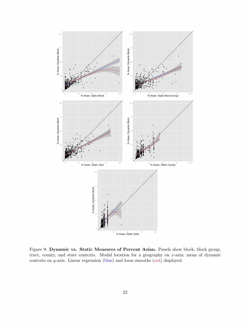
●
●
●
●
●
●
●
●
●
●
●
●
●
●●
●
●
●
●
●
●
●
●
●
●
●
●●
●
●
●
●
●
●
●
● ●
●
●
●
●
●
●
●
●
●
●●●
●●
●
●
●
●
●
●●
●
●
●
●
●
●
●●
●
●
●
●
●
●
●●
●
●
●
●
●
●●
●
●●
●
●
●
●
●
●
●
●
●
●
●
●
●
●
●
●●
●
●
●
●
●
●
●
●
●
●
●
●●
●
●
●
●●
●
●
●●●
●
●●
●
●●●
●
●●
●
●
●
●●
●
●
●
●
●
●
●
●
●
●
●
●
●
●
●●
●
●
●
●
●
●
●
●
●
●
●
●
●
●
●
●
●
●
●●
●
●
●
●
●
●
●●
●
●
●
●
●
●
●
●
●
●
●
●
● ●
●
●●●
●
●
●
●
●
●
●
●
●●
●
●
●
●
●
●
●●
●
●
●
●
●
●
●
●
●●
●●
●
●
●
●
●
●
●●
●
●●
●
●
●
●
●
●
●
●●
●
●
●
●
●
●
●
●
●
●
●
●
●
●
●
●
●
●
●
●
●●
●
●
●
●●
●
●
●
●
●
●●
●
●
●
●
●
●
●●●
●
●
●
●
●
●●
●
●
●●
●
●
●
●
●
●
●●
●
●
●
●●
●
●
●
●
●●
●
●
●
●●
●
●●
●
●
●
●
●
●●
●
●
●
●●
●
●
●
●
●
●
●
● ● ●
●
●
●
●
●●
●●
●●
●
●
●
●
●
●
●
●
● ●
●
●●
●
●
●
●
●
●
●
●
●
●
0
25
50
75
100
0 25 50 75 100
% Asian, Static Block
% A
sian
, Dyn
amic
Blo
ck
●
●
●
●
●
●
●
●
●
●
●
●
●
●●
●
●
●
●
●
●
●
●
●
●
●
●●●
●
●
●
●
●
●
●
●●
●
●
●
●
●
●
●
●
●
●
●●●
●●
●
●
●
●
●
●●●
●
●●
●
●
●
●
●●
●
●
●
●
●
●
●●
●
●
●
●
●
●
●●
●
●●
●
● ●
●
●
●
●
●
●●
●
●
●
●
●
●
●
●
●●
●
●
●
●
●
●
●
●
●●
●
●
●
●●
●
●
●
●●
●
●
● ●●
●
●●
●
●●●
●
●
●
●●
●
●
●
●●
●
●
●
●
●
●
●
●
●
●
●
●
●
●
●
●●
●
●
●
●
●
●
●
●●
●
●
●
●
●
●
●
●●
●
●
●
●●
●
●
●
●
●
●
●●
●
●
●
●
●
●
●
●
●
●
●
●
● ●
● ●
●●●
●
●
●
●
●
●
●
●
●●
●
●
●
●
●
●
●
●●
●
●
●
●
●
●
●
●
●
●●
●●
●
●
●
●
●
●●●
●
●
●
●
●
●
●
●●
●
●
●
●
●
●●
●●
●
●
●
●
●
●
●
●
●
●
●
●
●
●
●
●
●
●●
●
●
●
●
●
●
●●
●
●
●
●●
●
●
●
●
●
●
●
●
●
●
●
●
●
●
●
●
●
●●●
●
●
●
●
●
●
●
●●
●
●●
●
●
●
●
●
●
● ●
●
●
●
●
●●
●
●
●
●
●
●
●
●
●
●
●●●
●●
● ●
●
●
●
●
●
●●
●
●
●
●
●●
●
●
●
●
●
●
●
● ●●
●
●
●
●
●●
●●
● ●
●
●
● ●
●
●
●
●
●
●●
●●
● ●
●●
●
●
●
●
●
●
●
●
●
●
●
●
●
0
25
50
75
100
0 25 50 75 100
% Asian, Static Block Group
% A
sian
, Dyn
amic
Blo
ck
●
●
●
●
●
●
●
●
●
●
●
●
●
●●
●
●
●
●
●
●
●
●
●
●
●
●
●●●
●
●
●
●
●
●
●
● ●
●
●
●
●
●
●
●
●
●
●
●●●
●●
●
●
●
●
●
●●●
●
●●
●
●
●
●
●●
●
●
●
●
●
●
●●
●
●
●
●
●
●
●●
●
●●
●
● ●
●
●
●
●
●
●●
●
●
●
●
●
●
●
●
●
●●
●
●
●
●
●
●
●
●
●●
●
●
●
●●
●
●
●
● ●
●
●
●●●
●
●●
●
●●●
●
●
●
●●
●
●
●
●●
●
●
●
●
●
●
●
●
●
●
●
●
●
●
●
●●
●
●
●
●
●
●
●
●
●●
●
●
●
●
●
●
●
●●
●
●
●
●●
●
●
●
●
●
●
● ●●
●
●
●
●
●
●
●
●
●
●
●
●
● ●
● ●
●●●
●
●
●
●
●
●
●
●
●●
●
●
●
●
●
●
●
●●
●
●
●
●
●
●
●
●
●
●●
●●
●
●
●
●
●
●
●●●
●
●
●
●
●
●
●
● ●
●
●
●
●
●
●●
●●
●
●
●
●
●
●
●
●
●
●
●
●
●
●
●
●
●
●●
●
●
●
●
●
●
●●
●
●
●
●●
●
●
●
●
●
●
●
●
●
●
●
●
●
●
●
●
●
●●●
●
●
●
●
●
●
●
●●
●
●●
●
●
●
●
●
●
● ●
●
●
●
●
● ●
●
●
●
●
●
●
●
●
●
●
●●●
●●
●●
●
●
●
●
●
●●
●
●
●
●
●●
●
●
●
●
●
●
●
● ● ●
●
●
●
●
●●
●●
●●
●
●
●●
●
●
●
●
●
●●
● ●
● ●
●●
●
●
●
●
●
●
●
●
●
●
●
●
●
0
25
50
75
100
0 25 50 75 100
% Asian, Static Tract
% A
sian
, Dyn
amic
Blo
ck
●
●
●
●
●
●
●
●
●
●
●
●
●
●●
●
●
●
●
●
●
●
●
●
●
●
●
●●●
●
●
●
●
●
●
●
●●
●
●
●
●
●
●
●
●
●
●
●●●
●●
●
●
●
●
●
●●●
●
●●
●
●
●
●
●●
●
●
●
●
●
●
●●
●
●●
●
●
●
●
●●
●
●●
●
●
●●
●
●
●
●
●
●●
●
●
●
●
●
●
●
●
●
●●
●
●
●
●
●
●
●
●
●●
●
●
●
●●
●
●
●
●●
●
●
●●●
●
●●
●
●●●
●
●
●
●●
●
●
●
●●
●
●
●
●
●
●
●
●
●
●
●
●
●
●
●
●●
●
●
●
●
●
●
●
●
●●
●
●
●
●
●
●
●
●●
●
●
●
●●
●
●
●
●
●
●
●●●
●
●
●
●
●
●
●
●
●
●
●
●
●
● ●
● ●
●●●
●
●
●
●
●
●
●
●
●●
●
●
●
●
●
●
●
●●
●
●
●
●
●
●
●
●
●
●●
●●
●
●
●
●
●
●
●●●
●
●
●
●
●
●
●
●●
●
●
●
●
●
●●
●●
●
●
●
●
●
●
●
●
●
●
●
●
●
●
●
●
●
●●
●
●
●
●
●
●
●●
●
●
●
●●
●
●
●
●
●
●
●
●
●
●
●
●
●
●
●
●
●
●●●
●
●
●
●
●
●
●
●●
●
●●
●
●
●
●
●
●
●●
●
●
●
●
●●
●
●
●
●
●
●
●
●
●
●
●●●
●●
●●
●
●
●
●
●
●
●●
●
●
●
●
●●
●
●
●
●
●
●
●
●● ●
●
●
●
●
●●
● ●
●●
●
●
● ●
●
●
●
●
●
●●
●●
● ●
●●
●
●
●
●
●
●
●
●
●
●
●
●
●
●
0
25
50
75
100
0 25 50 75 100
% Asian, Static County
% A
sian
, Dyn
amic
Blo
ck
●
●
●
●
●
●
●
●
●
●
●
●
●
●●
●
●
●
●
●
●
●
●
●
●
●
●
●●●
●
●
●
●
●
●
●
●●
●
●
●
●
●
●
●
●
●
●
●●●
●●
●
●
●
●
●
●●●
●
●●
●
●
●
●
●●
●
●
●
●
●
●
●●
●
●●
●
●
●
●
●●
●
●●
●
●
● ●
●
●
●
●
●
●●
●
●
●
●
●
●
●
●
●
● ●
●
●
●
●
●
●
●
●
●●
●
●
●
●●
●
●
●
●●
●
●
● ●●
●
●●
●
●●●
●
●
●
●●
●
●
●
●●
●
●
●
●
●
●
●
●
●
●
●
●
●
●
●
●●
●
●
●
●
●
●
●
●
●●
●
●
●
●
●
●
●
●●
●
●
●
●●
●
●
●
●
●
●
●●●
●
●
●
●
●
●
●
●
●
●
●
●
●
● ●
● ●
●●●
●
●
●
●
●
●
●
●
●●●
●
●
●
●
●
●
●●
●
●
●
●
●
●
●
●
●
●●
●●
●
●
●
●
●
●
●●●
●
●
●
●
●
●
●
●●
●
●
●
●
●
●●
●●
●
●
●
●
●
●
●
●
●
●
●
●
●
●
●
●
●
●●●
●
●
●
●
●
●●
●
●
●
● ●
●
●
●
●
●
●
●
●
●
●
●
●
●
●
●
●
●
●●●
●
●
●
●
●
●
●
●●
●
●●
●
●
●
●
●
●
●●
●
●
●
●
●●
●
●
●
●
●
●
●
●
●
●
●●●
●●
●●
●
●
●
●
●
●
●●
●
●
●
●
●●
●
●
●
●
●
●
●
●●●
●
●
●
●
●●
● ●
●●
●
●
●●
●
●
●
●
●
●●
●●
● ●
●●
●
●
●
●
●
●
●
●
●
●
●
●
●
●
0
25
50
75
100
0 25 50 75 100
% Asian, Static State
% A
sian
, Dyn
amic
Blo
ck
Figure 9: Dynamic vs. Static Measures of Percent Asian. Panels show block, block group,tract, county, and state contexts. Modal location for a geography on x-axis; mean of dynamiccontexts on y-axis. Linear regression (blue) and loess smooths (red) displayed.
22
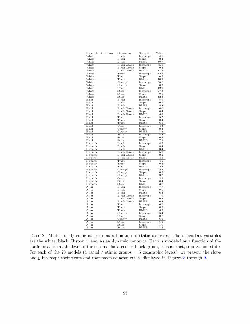
Race Ethnic Group Geography Statistic ValueWhite Block Intercept 34.1White Block Slope 0.4White Block RMSE 10.7White Block Group Intercept 35.6White Block Group Slope 0.4White Block Group RMSE 11.3White Tract Intercept 32.2White Tract Slope 0.5White Tract RMSE 10.9White County Intercept 35.2White County Slope 0.5White County RMSE 12.0White State Intercept 27.3White State Slope 0.6White State RMSE 12.3Black Block Intercept 5.9Black Block Slope 0.5Black Block RMSE 5.8Black Block Group Intercept 6.0Black Block Group Slope 0.4Black Block Group RMSE 6.3Black Tract Intercept 5.7Black Tract Slope 0.4Black Tract RMSE 6.5Black County Intercept 4.4Black County Slope 0.4Black County RMSE 7.2Black State Intercept 4.8Black State Slope 0.4Black State RMSE 7.9Hispanic Block Intercept 4.2Hispanic Block Slope 0.4Hispanic Block RMSE 3.4Hispanic Block Group Intercept 5.0Hispanic Block Group Slope 0.2Hispanic Block Group RMSE 4.2Hispanic Tract Intercept 4.5Hispanic Tract Slope 0.3Hispanic Tract RMSE 3.8Hispanic County Intercept 2.8Hispanic County Slope 0.5Hispanic County RMSE 3.2Hispanic State Intercept 2.9Hispanic State Slope 0.4Hispanic State RMSE 3.8Asian Block Intercept 7.7Asian Block Slope 0.5Asian Block RMSE 6.4Asian Block Group Intercept 7.9Asian Block Group Slope 0.4Asian Block Group RMSE 6.8Asian Tract Intercept 6.7Asian Tract Slope 0.5Asian Tract RMSE 6.2Asian County Intercept 5.4Asian County Slope 0.7Asian County RMSE 6.5Asian State Intercept 5.2Asian State Slope 1.0Asian State RMSE 7.4
Table 2: Models of dynamic contexts as a function of static contexts. The dependent variablesare the white, black, Hispanic, and Asian dynamic contexts. Each is modeled as a function of thestatic measure at the level of the census block, census block group, census tract, county, and state.For each of the 20 models (4 racial / ethnic groups × 5 geographic levels), we present the slopeand y-intercept coefficients and root mean squared errors displayed in Figures 3 through 9.
23
References
Asakura, Yasuo, and Eiji Hato. 2004. “Tracking survey for individual travel behaviour using mobilecommunication instruments.” Transportation Research Part C 12(3–4): 273–291.
Baybeck, Brady. 2006. “Sorting Out the Competing Effects of Racial Context.” Journal of Politics68(2): 386–396.
Baybeck, Brady, and Robert Huckfeldt. 2002. “Spatially dispersed ties among interdependentcitizens: connecting individuals and aggregates.” Political Analysis 10(3): 261–275.
Berger, Jonah, Marc Meredith, and S. Christian Wheeler. 2008. “Contextual Priming: WherePeople Vote Affects How They Vote.” Proceedings of the National Academy of Sciences 105(26):8846–8849.
Berry, William D., and Brady Baybeck. 2005. “Using Geographic Information Systems to StudyInterstate Competition.” American Political Science Review 99(November): 505–519.
Bledsoe, Timothy, Susan Welch, Lee Sigelman, and Michael Combs. 1995. “Residential Contextand Racial Solidarity among African Americans.” American Journal of Political Science 39(May):434–458.
Carsey, Thomas M. 1995. “The Contextual Effects of Race on White Voter Behavior: The 1989New York City Mayoral Election.” Journal of Politics 57(February): 221–228.
Cho, Wendy K. Tam, and James G. Gimpel. 2012. “Geographic Information Systems and theSpatial Dimensions of American Politics.” Annual Review of Political Science 15(1).
Cho, Wendy K. Tam, and Neil Baer. 2011. “Environmental Determinants of Racial AttitudesRedux: The Critical Decisions Related to Operationalizing Context.” American Politics Research39(2): 414–436.
Cho, Wendy K. Tam, James G. Gimpel, and Daron R. Shaw. 2012. “The Tea Party Movement andthe Geography of Collective Action.” Quarterly Journal of Political Science 7: 105–133.
Cho, Wendy K Tam, James G Gimpel, and Joshua J Dyck. 2006. “Residential Concentration,Political Socialization, and Voter Turnout.” Journal of Politics 68(1): 156–167.
Christiansen, Martin Bisgaard, Kim Mannemar Sønderskov, and Peter Thisted Dinesen. 2016.“Reconsidering the Neighborhood Effect: Does Exposure to Residential Unemployment InfluenceVoters’ Perceptions of the National Economy?” Journal of Politics .
Congdon, Peter. 2009. “A multilevel model for cardiovascular disease prevalence in the US andits application to micro area prevalence estimates.” International Journal of Health Geographics8(6): 1–14.
Dinesen, Peter Thisted, and Kim Mannemar Sønderskov. 2015. “Ethnic Diversity and Social Trust:Evidence from the Micro-Context.” American Sociological Review 80(3): 550–573.
Dixon, Jeffrey. 2006. “The Ties That Bind and Those That Don’t: Toward Reconciling GroupThreat and Contact Theories of Prejudice.” Social Forces 84(4): 2179–2204.
24
Eagle, Nathan, Alex (Sandy) Pentland, and David Lazer. 2009. “Inferring friendship networkstructure by using mobile phone data.” Proceedings of the National Academy of Sciences 106(36):15274–15278.
Eulau, Heinz, and Lawrence Rothenberg. 1986. “Life Space and Social Networks as Political Con-texts.” Political Behavior 8(2): 130–157.
Ford, Scott W. 1973. “Interracial Public Housing in a Border City: Another Look at the ContactHypothesis.” American Journal of Sociology 78(6): 1426–1447.
Fosset, Mark, and K. Jill Kiecolt. 1989. “The Relative Size of Minority Populations and WhiteRacial Attitudes.” Social Science Quarterly 70(4): 820–835.
Gasper, John T., and Andrew Reeves. 2011. “Make it Rain? Retrospection and the AttentiveElectorate in the Context of Natural Disasters.” American Journal of Political Science 55(2):340–355.
Giles, Michael, and Arthur Evans. 1986. “The Power Approach to Intergroup Hostility.” TheJournal of Conflict Resolution 30(3): 469–486.
Gilliam, Franklin D., Nicholas Valentino, and Matthew Beckmann. 2002. “Where You Live andWhat You Watch: The Impact of Racial Proximity and Local Television News on AttitudesAbout Race and Crime.” Political Research Quarterly 55(4): 755–780.
Gimpel, James G., Nathan Lovin, Bryant Moy, and Andrew Reeves. Forthcoming. “The Urban-Rural Gulf in American Political Behavior.” Political Behavior .
Glaser, James M. 1994. “Back to the Black Belt: Racial Environment and White Racial Attitudesin the South.” The Journal of Politics 56(01): 21–41.
Green, Donald P., Dara Z. Strolovitch, and Janelle S. Wong. 1998. “Defended Neighborhoods,Integration, and Racially Motivated Crime.” American Journal of Sociology 104(2): 372–403.
Hero, Rodney E., and Caroline J. Tolbert. 2004. “Minority Voices and Citizen Attitudes aboutGovernmental Responsiveness in the American States: Do Social and Institutional ContextsMatter?” British Journal of Political Science 34(1): 109–121.
Hjorth, Frederik, Peter Thisted Dinesen, and Kim Mannemar Sønderskov. 2016. The Content andCorrelates of Subjective Local Contexts. In Proceedings of the Annual Meeting of the AmericanPolitical Science Association.
Hopkins, Daniel J. 2010. “Politicized Places: Explaining Where and When Immigrants ProvokeLocal Opposition.” American Political Science Review 104(1): 40–60.
Hopkins, Daniel J. 2013. “Misplaced: The Limits of Contextual Influence on Americans’ PoliticalAttitudes.” (Typescript).
Huckfeldt, R. Robert. 1979. “Political Participation and the Neighborhood Social Context.” Amer-ican Journal of Political Science 23(3): 579–592.
25
Huckfeldt, R. Robert. 1986. Politics In Context: Assimilation and Conflict in Urban Neighborhoods.Vol. New York, NY Agathon Press, Inc.
Key, Valdimer Orlando. 1949. Southern Politics in State and Nation. Knoxville: University ofTennessee Press.
King, Gary. 1996. “Why Context Should Not Count.” Political Geography 15: 159–164.
Kriner, Douglas L., and Andrew Reeves. 2012. “The Influence of Federal Spending on PresidentialElections.” American Political Science Review 106(2): 348–366.
Kriner, Douglas L., and Andrew Reeves. 2015. “Presidential Particularism and Divide-the-DollarPolitics.” American Political Science Review 109(1): 155–171.
Kwan, Mei-Po. 1998. “Space-Time and Integral Measures of Individual Accessibility: A Compara-tive Analysis Using a Point-based Framework.” Geographical Analysis 30(3): 191–216.
Kwan, Mei-Po. 1999. “Gender and Individual Access to Urban Opportunities: A Study UsingSpace-Time Measures.” The Professional Geographer 51(2): 210–227.
Kwan, Mei-Po. 2009. “From place-based to people-based exposure measures.” Social Science &Medicine 69(9): 1311–1313.
Kwan, Mei-Po. 2012. “The Uncertain Geographic Context Problem.” Annals of the Association ofAmerican Geographers 102(5): 958–968.
MacKuen, Michael, and Courtney Brown. 1987. “Political Context and Attitude Change.” Ameri-can Political Science Review 81(2): 471–490.
Massey, Douglas S, and Nancy A. Denton. 1993. American Apartheid: Segregation and the Makingof the Underclass. Cambridge, MA: Harvard University Press.
Matthews, Stephen A. 2008. “The Salience of Neighborhood: Some Lessons from Sociology.”American Journal of Preventive Medicine 34(3): 257–259.
McLaughlin, Diane K., and C. Shannon Stokes. 2002. “Income inequality and mortality in UScounties: does minority racial concentration matter?” American Journal of Public Health 92(1):99–104.
Mellor, Jennifer M., and Jeffrey D. Milyo. 2004. “Individual health status and racial minorityconcentration in US states and counties.” American Journal of Public Health 94(6): 1043–1048.
Mennis, Jeremy, and Michael J. Mason. 2012. “Social and geographic contexts of adolescent sub-stance use: The moderating effects of age and gender.” Social Networks 34(1): 150–157.
Moore, Ryan T., and Andrew Reeves. 2017. “Learning from Place in the Era of Geolocation.” InAnalytics, Policy and Governance, ed. Jennifer Bachner, Kathryn Wagner Hill, and BenjaminGinsberg. Yale University Press pp. 118–136.
Moore, Ryan T., and Andrew Reeves. 2020. Replication Data for: Defining Racial and EthnicContext with Geolocation Data. Harvard Dataverse.
26
Moore, Ryan T., and Nirmala Ravishankar. 2012. “Who Loses in Direct Democracy?” SocialScience Research 41(May): 646–656.
Morris, Irwin. 2000. “African American Voting on Proposition 187: Rethinking the Prevalence ofInterminority Conflict.” Political Research Quarterly 53(1): 77–98.
Mutz, Diana C., and Jeffrey J. Mondak. 2006. “The Workplace as a Context for Cross-CuttingPolitical Discourse.” Journal of Politics 68(1): 140–155.
Oliver, Eric J., and Janelle Wong. 2003. “Intergroup Prejudice in Multiethnic Settings.” AmericanJournal of Political Science 47(4): 567–582.
Oliver, Eric J., and Tali Mendelberg. 2000. “Reconsidering the Environmental Determinants ofWhite Racial Attitudes.” American Journal of Political Science 44(July): 574–589.
Palmer, John R. B., Thomas J. Espenshade, Frederic Bartumeus, Chang Y. Chung, Necati ErcanOzgencil, and Kathleen Li. 2013. “New Approaches to Human Mobility: Using Mobile Phonesfor Demographic Research.” Demography 50(3): 1105–1128.
Peffley, Mark, Marc L. Hutchison, and Michal Shamir. 2015. “The Impact of Persistent Terrorismon Political Tolerance: Israel, 1980 to 2011.” American Political Science Review 109(4): 817–832.
Reeves, Andrew, and James G. Gimpel. 2012. “Ecologies of Unease: Geographic Context andNational Economic Evaluations.” Political Behavior 34(3): 507–534.
Solt, Frederick. 2010. “Does Economic Inequality Depress Electoral Participation? Testing theSchattschneider Hypothesis.” Political Behavior 32(2): 285–301.
South, Scott J. 2001. “The Geographic Context of Divorce: Do Neighborhoods Matter?” Journalof Marriage and Family 63(3): 755–766.
Stein, Robert M., Stephanie Shirley Post, and Allison L. Rinden. 2000. “Reconciling Contact andContext Effects on Racial Attitudes.” Political Research Quarterly 53(2): 285–303.
Stolle, Dietlind, Stuart Soroka, and Richard Johnston. 2008. “When Does Diversity Erode Trust?Neighborhood Diversity, Interpersonal Trust and the Mediating Effect of Social Interactions.”Political Studies 56(1): 57–75.
Taylor, Marylee C. 1998. “How White Attitudes Vary with the Racial Compositions of LocalPopulations: Numbers Count.” American Sociological Review 63(4): 512–535.
Tufte, Edward R. 1973. “The Relationship between Seats and Votes in Two-Party Systems.” TheAmerican Political Science Review 67(2): 540–554.
Velez, Yamil, and Grace Wong. 2016. “Assessing Contextual Measurement Strategies.” Manuscript.
Weber, Christopher R., Howard Lavine, Leonie Huddy, and Christopher M. Federico. 2014. “PlacingRacial Stereotypes in Context: Social Desirability and the Politics of Racial Hostility.” AmericanJournal of Political Science 58(January): 63–78.
27
Wong, Cara, Jake Bowers, Daniel Rubenson, Mark Fredrickson, and Ashlea Rundlett. 2013. “Doesthe Context Fit the Outcome? When (or Where) Racial/Ethnic Context Should Affect Politics.”American Political Science Association annual meeting.
Wong, Cara, Jake Bowers, Daniel Rubenson, Mark Fredrickson, and Ashlea Rundlett. 2015. “DoYou See What I See?: Psuedoenvironments, Ethnic Diversity, and Social Capital.” Manuscript.(August).
Wong, Cara, Jake Bowers, Daniel Rubenson, Mark Fredrickson, and Ashlea Rundlett. 2016. “Mapsin People’s Heads as a New Measure of Context.” Manuscript.
Wong, Cara, Jake Bowers, Tarah Williams, and Katherine Drake Simmons. 2012. “Bringing thePerson Back In: Boundaries, Perceptions, and the Measurement of Racial Context.” Journal ofPolitics 74(4): 1153–1170.
Wright, Gerald C. 1976. “Community Structure and Voting in the South.” Public Opinion Quarterly40(2): 201–215.
Zandbergen, Paul A. 2009. “Accuracy of iPhone Locations: A Comparison of Assisted GPS, WiFiand Cellular Positioning.” Transactions in GIS 13: 5–25.
28