Embed Size (px)
Citation preview
De Facto Currency Baskets of China and East Asian Economies: The Rising
Weights
Ying Fanga, Shicheng Huanga, Linlin Niua,b,∗
aWang Yanan Institute for Studies in Economics (WISE), Xiamen UniversitybBank of Finland’s Institute for Economies in Transition
Abstract
We employ a Bayesian method to estimate a time-varying coefficient version of the de facto currency
basket model of Frankel and Wei (2007) for the RMB of China, using daily data from February 2005 to
July 2011. We estimate jointly the implicit time-varying weights of all 11 currencies in the reference basket
announced by the Chinese government. We find the dollar weight has been reduced and is sometimes
significantly smaller than one, but there is no evidence of systematic operation of a currency basket with
a discernable pattern of significant weights on other currencies. During specific periods, the reduced
dollar weight has not been switched to other major international currencies, but instead to some East
Asian currencies, which is hard to explain by trade importance to or trade competition with China. We
examine currency baskets of these East Asian Economies, which include major international currencies
and the RMB in their baskets. We find an evident tendency of Malaysia and Singapore to increase the
weights of RMB in their own currency baskets, and a continuously significant positive weight of RMB
in the basket of Thailand. These findings suggest that the occasionally positive weights of some East
Asian currencies in RMB currency basket reflects the positive RMB weights in these East Asian currency
baskets, as these East Asian economies have been systematically placing greater weights on RMB under
the new regime of RMB exchange rate.
Keywords: RMB currency basket, time-varying regressions, East Asia, China, US
∗Corresponding author. Address: WISE, Economics Building A301, Xiamen University, 361005, Xiamen, China. E-Mail: [email protected]. Telephone: +86-592-2182839. Fax: +86-592-2187708.
Email addresses: [email protected] (Ying Fang), [email protected] (Shicheng Huang),[email protected] (Linlin Niu)
1. Introduction
One of the central economic issues of the past decade is global imbalance, which features substantial
US deficits and Chinese surpluses. Much of the related concern is about China’s exchange rate regime.
The international consensus and pressure are for China’s currency, the yuan (RMB), to appreciate, but
there is no easy answer concerning the proper extent of appreciation. While the Chinese government
has allowed the RMB to float within a narrow band since July 2005, the pace of adjustment is slow
and the mechanism lacks of transparency. Understanding the changing regime and its significance are
of great importance to the international community. This paper sheds light on these issues following a
brief review of the background and related research.
The remarkable economic boom of China has been one of the most important economic phenomena
of the past three decades. In 1978 when China launched economic reform, the total volume of China’s
foreign trade was a mere of $21 billion. It increased to $1.1 trillion in 2004 (Branstetter and Lardy,
2008), equivalent to an average annual growth rate of 15% for more than two decades. China has become
the second largest economy in terms of GDP, trade volume and the volume of foreign direct investment.
Meanwhile, China has long operated a dollar-pegged exchange rate regime, even after a highly successful
opening up to foreign trade and investment. For example, the USD/CNY exchange rate was almost fixed
around 8.3 from 1995 to the summer of 2005. A rigid exchange rate regime has been blamed for the huge
current account surpluses with respect to the US, which is a central issue in global imbalance. Since
2003, China has encountered intense pressure to appreciate the RMB.
On July 21, 2005, China’s monetary authority announced its establishment of a managed floating
exchange rate regime, as it moved from a dollar-pegged regime to the one based on a basket of several
currencies to determine the value of RMB. About half a month later, Mr. Xiaochuan Zhou, the governor
of People’s Bank of China, claimed on August 9 that the basket would contain 11 currencies: the US
dollar (USD), Japanese yen (JPY), euro (EUR), South Korean won (KRW), Australian dollar (AUD),
Canadian dollar (CAD), British pound (GBP), Malaysia ringgit (MYR), Russian ruble (RUB), Singapore
dollar (SGD) and the Thailand baht (THB). The governor emphasized that the first four currencies would
play more important roles in determining the value of RMB. In addition, the daily floating band for the
exchange rates was set at ±0.3% around the central parity. This band was widened to ±0.5% on May 21,
2007. Figure 1 shows the level and log difference of USD/RMB exchange rate daily data from February
2
2005 to July 2011. The figure reveals different stages of the exchange rate dynamics resulting from hidden
policy operations.
[Figure 1. Level and Log-difference of RMB/USD Exchange Rate]
The aforementioned policy change has attracted much attention in assessing China’s de facto exchange
rate regime. For example, Shah and Patnaik (2005) found no evidence to support a basket peg in the
daily Chinese exchange rates from July to October in 2005. Extending the data coverage toJanuary
2006, Ogawa and Sakane (2006) found a statistically significant but small change in China’s policy for
the RMB/USD exchange rate, whereas the currency basket system was not explored in their paper.
Frankel and Wei (2007) is the first paper to assess China’s de facto exchange rate regime and to identify
the implicit weights of other currencies in the basket, to determine the value of the RMB. By regressing
changes in the logarithm value of the RMB on changes in the logarithm values of the candidate currencies,
Frankel and Wei (2007) showed that, from July 2005 to the end of 2006, the weight of the USD was still
fairly heavy, although some Asian currencies load significantly positvely in the subsamples of the first
half of 2006. Furthermore, they found some empirical evidence that the implicit weight of the USD was
related to the pressure from the bi-annual US Treasury reports. Extending the examination period to
2007, Frankel and Wei (2008) found that a simple dollar peg regime dominates over most of the period.
Frankel (2009) found evidence that, during the period from July 2005 to 2008, the RMB basket began a
substantial switching of weight from USD to EUR, KRW or JPY, when only these four major currencies
were included in the regression; but when other currencies were included, the MYR became the most
influential after the USD. Finally, Fidrmuc (2010) estimated the implicit time-varying weights of three
international currencies in the RMB basket by Maximum Likelihood estimation (MLE) with Kalman
filter for the daily exchange rates in levels from March 2005 to January 2009, and found evidence of
flexibility at first but a reversal to a dollar peg since 2008.
The previous literature indicates that the currency weights of the RMB basket are time-changing and
that the sample periods and currency choices are important for the results. In this paper, we employ the
random coefficient model to identify the time-varying de facto weights of the RMB currency basket using
daily exchange rate data from February 2005 to July 2011. Although the USD weight was overwhelmingly
heavy during most of the sample period, we find evidence that the USD weight has been reduced and was
3
at times significantly less than one. In particular, we find that much of the lost weight on USD moved
to the weights on some Asian currencies rather than to the major international currencies such as EUR,
JPY or GBP.
The significant Asian currency weights found in our study echo some sets of results in Frankel and Wei
(2007) in that only weights of USD and MRY were significant in their sample between 2005 and 2007.
But the explanation of the significance of MRY weight is not convincing in the paper. In our paper,
we look at this issue from the side of East Asian economies in the potential adjustment of their own
currency basket weights under the backdrop of China’s changing exchange rate regime, and find firm
evidence that the RMB has become increasingly important in determining the Asian currency values.
We find a tendency of Malaysia and Singapore to increase the weights of RMB in their own currency
baskets, and a continuously significant positive weight of RMB in the basket of Thailand. The results
explain the positive coefficients in a bilateral regression when the RMB currency value is the dependent
variable and the Asian currency values are explanatory variables. Despite the lack of transparency in
the currency basket of China, these Asian economies have swiftly prepared themselves for a more flexible
RMB.
Compared to the existing literature, our paper contributes in three ways. Firstly, the random coefficient
model adopted in the paper can not only efficiently utilize the whole sample information but can also
accommodate the time-varying features. While learning about the evolution of China’s de facto exchange
rate regime is of capital importance in this literature, most existing studies estimate the time-varying
weights by using sub-samples and rolling regressions, which are subject to information inefficiency of
short sample and biased estimates due to uncertainties in subsample division. In a transition from
fixed exchange rate to a more flexible regime, both smoothed change and abrupt breaks can happen in
the process such that the constant coefficient model is subject to biased estimator. For example, Cai,
Chen and Fang (2012) detected some structural breaks in the daily log return of Chinese exchange rate.
The random coefficient model used in this paper is not only capable of capturing smoothed change in
parameters, but can also detect sudden breaks effectively, by fully utilizing the whole sample information.
Secondly, by including all eleven currencies in the officially announced currency basket of RMB and
using a Bayesian sampling method, our paper avoids some potential problems of Fidrmuc (2010), where
only three international currencies are included in the time-varying regression using Maximum Likelihood
4
Estimation (MLE) with Kalman filter. Excluding relevant currencies in the basket may lead to the
problem of omitted variables. The MLE using Kalman filter encounters numerical difficulty regarding
high dimension optimization, when a large set of latent variables, i.e. currency weights, are involved.
Lastly, our paper echoes the debate in the literature about whether and why some Asian currencies gain
the lost weight on the USD, even though they are not strategically as important as the major international
currencies in terms of both trade and capital flows. We attribute the phenomenon of increasing weights
on these Asian currencies to the tendency of these Asian emerging markets to increase the weight of the
RMB in their own currency baskets. The results provide insight into the influence and consequence of
the changing regime of China’s exchange rate.
The rest of the paper is organized as follows. Section 2 presents the time-varying coefficient regression
for currency basket with a model of the RMB currency basket and a model of the currency basket for
Asian economies, as well as the estimation methodology. Section 3 describes the data. Section 4 presents
the estimation results. Section 5 concludes.
2. Time-varying Coefficient Regressions for Currency Basket
2.1. Model of RMB Currency Basket
2.1.1. Linear Model with Constant Coefficients
To discover the opaque currency basket weights of RMB, Frankel and Wei (2007, 2008) and Frankel
(2009) regressed the change in RMB exchange rate with respect to a numeraire on changes in exchange
rates of the basket currencies with respect to the same numeraire. A candidate numeraire currency is
the SDR. To allow for the likelihood of trend appreciation, a constant term is included in the regression.
∆ logRMBt = c+∑
wj [∆ logXj,t]
= c+ α∆ logUSDt + β1∆ logEURt + β2∆ logGBPt + β3...+ ut (1)
where α, β1, β2...βn are currency weights. Frankel and Wei (2008) include a detailed discussion of this
setup. When there is no clear information on the composition of the basket available, major international
currencies are usually included as regressors.
Assuming that the explanatory variables are all the currencies in the basket, the weights should sum
up to one, so that α = 1− β1 − β2... − βn holds as a constraint, under which the above equation can be
5
transformed to the following OLS regression by subtracting ∆ logUSDt from both sides
∆ logRMBt −∆ logUSDt
= c+ β1 [∆ logEURt −∆ logUSDt] + β2 [∆ logGBPt −∆ logUSDt] + β3...+ ut. (2)
In this transformed equation, the left hand side is the change in RMB/USD, and the right hand side
involves changes in exchange rates of other currencies with respect to the USD. Frankel and Wei (2008)
obtained similar results in the unconstrained and constrained regressions.
Frankel and Wei (2007) and Frankel (2009) estimated the weights for several subsamples to uncover
the patterns of the weight changes in the RMB currency basket. However, the results are dependent on
the choice of sample division and influenced by sudden events in the subsamples.
2.1.2. Time-varying Coefficient Model
To overcome the problems of subsample OLS regressions and efficiently utilize the information of the
whole sample, we employ time-varying coefficient regression to model the dynamic weights of the basket
currencies:
∆ logRMBt = ct + αt∆ logUSDt + β1t∆ logEURt + β2t∆ logGBPt + β3t...+ ut. (3)
Since we assume that for China the equation includes all relevant currencies in the basket so that sum
of weights is equal to 1, αt = 1− β1t − β2t... − βnt, we obtain the time-varying coefficient model
∆ logRMBt −∆ logUSDt
= ct + β1t [∆ logEURt −∆ logUSDt] + β2t [∆ logGBPt −∆ logUSDt] + β3t...+ ut. (4)
We assume that the time-varying parameters of currency weights follow a random walk process:
βjt = βjt−1 + εjt (5)
with var(εjt) = σ2εj. The random walk is appropriate to model the dynamics when there are possible
structural changes or nonstationary trend, which are highly likely in a transition from a pegged to USD
exchange rate to managed floating with respect to a currency basket.
As for the intercept ct, which reflects adjustment speeds when the RMB value trended steadily, we
use a dummy variable to incorporate the characteristics of two visible regime trends of the RMB/USD
6
exchange rate. As shown in Figure 1, there are two types of periods: periods of modest appreciation
at roughly constant speed, from July 10, 2005 to July 10, 2008, and from June 22, 2010 onwards; and
periods of zero trend, before July 10, 2005 and from July 11, 2008 to June 21, 2010, which resembled a
fixed exchange rate period. Thus we introduce a dummy dt such that ct = α1 +α2dt, with dt = 1 for the
first type, and dt = 0 for the second type. If we do not introduce the dummy dt, ct = α1 and we have
the constant term case as in Frankel and Wei (2007)1.
2.2. Currency Basket Model for Asian economies
We will use the unconstrained representation to study how the Asian currency values have targeted
at international currencies and the RMB since July 2005, when RMB became more flexible with respect
to the dollar. This exercise will help us to understand the “puzzling” result of currency weights in the
officially announced RMB basket, as noticed by Frankel and Wei (2007). In these regressions, we explain
the value change in an Asian currency by weighted value changes in international currencies, USD, EUR,
JPY and GBP, and the RMB.
Taking the Korean won as an example, the regression equation is
∆ logKRWt = c+ β1t∆ logUSDt + β2t∆ logEURt + β3t∆ log JPYt + β4t∆ logGBPt
+β5t∆ logCNYt + ut. (6)
This unrestricted setup is more appropriate than the constrained one, as we do not have information
on the exact basket currencies. Again we model the time-varying weights as random walk processes.
Since we do not have information on the possible trends of exchange rates in these economies, we keep c
constant.
2.3. Estimation of the Time-varying Coefficient Model of Currency Baskets
Given the dynamics of the weights, equations (4) and (5) fit naturally into the state-space framework.
The states here are the time-varying weights evolving as random walks. The time-varying latent states
can be estimated by Kalman filter in the traditional Maximum Likelihood estimation (MLE). However,
1In fact, whether introducing a dummy for the intercept c or keeping it constant the results are fairly similar to those
for the time-varying weights. This indicates that once we allow currency weights to be time-varying, the adjustment speed
of change in exchange rate is incorporated in the changes in weights. We will report the results of both cases.
7
due to the high dimensionality of this system where a total of eleven state variables need to be filtered
out, MLE is subject to enormous difficulty with the numerical computation of the global optimum. To
overcome this problem, we utilize Bayesian inference with a Gibbs sampler to elicit posterior distributions
of the parameters and latent variables under proper prior assumptions and data information.
We choose the normal-gamma distribution for the prior distribution of α1 and α2, i.e., αi ∼ N(µ̄i,σ2αi)
and σ2αi
∼ Gamma(n, σ̄2i ) for i = 1, 2. The posterior distribution will also be normal-gamma. We set
prior distributions of variance parameters of σ2u and σ2
ε as Gamma distributions, which produce posterior
Gamma distributions. These parameters can be taken as random draws directly. A Kalman filter step
for filtering the latent states is embedded in the Gibbs sampler, and we use the algorithm of DeJong and
Shephard (1995) to draw from the posterior distributions of time-varying weights. The hyperparameters
of prior distributions for the time-varying latent weights are set at relatively high values, which allows
them to vary widely over time.
3. Data
The currency basket of China’s yuan (RMB) includes the US dollar (USD), Japanese yen (JPY), euro
(EUR), South Korean won (KRW), Australian dollar (AUD), Canadian dollar (CAD), British pound
(GBP), Malaysia ringgit (MYR), Russian ruble (RUB), Singapore dollar (SGD) and the Thailand baht
(THB). We take the Special Drawing Rights (SDR) as the reference currency. Daily data of the exchange
rates from February 7th, 2005 to July 29th, 2011 are downloaded from Bloomberg. Table 1 provides the
descriptive statistics for the log-differences of the selected exchange rates.
We test for stationarity using the ADF as well as KPSS test, and test for cointegration using Johansen
test under the null of a constant term. Table 2 presents the results for the unit root and stationarity
tests, and table 3 reports the cointegration test results. The ADF and KPSS test statistics indicate
that all the exchange rate levels are unit root processes, while the log returns of the exchange rates are
stationary. Results of the Johansen test show that there exists a single cointegration relation among
these currencies. These test statistics are reassuring for the econometric models that we estimate.
8
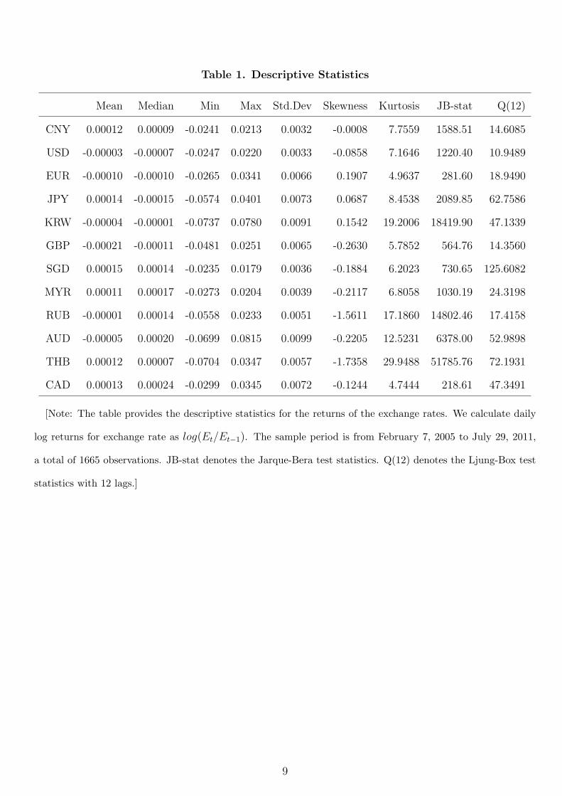
Table 1. Descriptive Statistics
Mean Median Min Max Std.Dev Skewness Kurtosis JB-stat Q(12)
CNY 0.00012 0.00009 -0.0241 0.0213 0.0032 -0.0008 7.7559 1588.51 14.6085
USD -0.00003 -0.00007 -0.0247 0.0220 0.0033 -0.0858 7.1646 1220.40 10.9489
EUR -0.00010 -0.00010 -0.0265 0.0341 0.0066 0.1907 4.9637 281.60 18.9490
JPY 0.00014 -0.00015 -0.0574 0.0401 0.0073 0.0687 8.4538 2089.85 62.7586
KRW -0.00004 -0.00001 -0.0737 0.0780 0.0091 0.1542 19.2006 18419.90 47.1339
GBP -0.00021 -0.00011 -0.0481 0.0251 0.0065 -0.2630 5.7852 564.76 14.3560
SGD 0.00015 0.00014 -0.0235 0.0179 0.0036 -0.1884 6.2023 730.65 125.6082
MYR 0.00011 0.00017 -0.0273 0.0204 0.0039 -0.2117 6.8058 1030.19 24.3198
RUB -0.00001 0.00014 -0.0558 0.0233 0.0051 -1.5611 17.1860 14802.46 17.4158
AUD -0.00005 0.00020 -0.0699 0.0815 0.0099 -0.2205 12.5231 6378.00 52.9898
THB 0.00012 0.00007 -0.0704 0.0347 0.0057 -1.7358 29.9488 51785.76 72.1931
CAD 0.00013 0.00024 -0.0299 0.0345 0.0072 -0.1244 4.7444 218.61 47.3491
[Note: The table provides the descriptive statistics for the returns of the exchange rates. We calculate daily
log returns for exchange rate as log(Et/Et−1). The sample period is from February 7, 2005 to July 29, 2011,
a total of 1665 observations. JB-stat denotes the Jarque-Bera test statistics. Q(12) denotes the Ljung-Box test
statistics with 12 lags.]
9
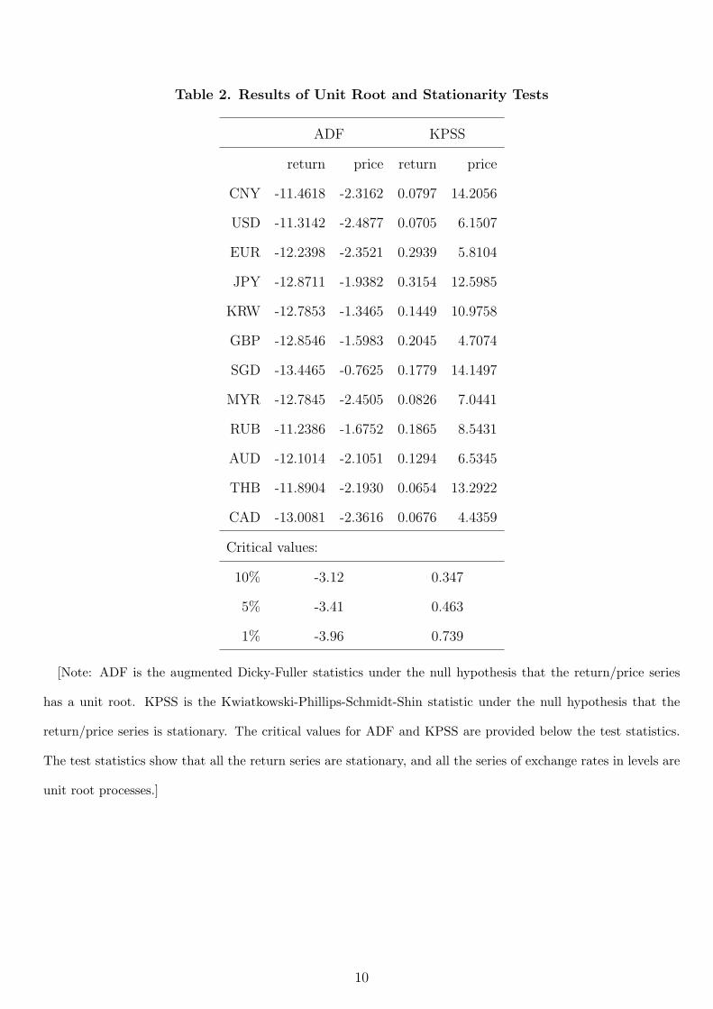
Table 2. Results of Unit Root and Stationarity Tests
ADF KPSS
return price return price
CNY -11.4618 -2.3162 0.0797 14.2056
USD -11.3142 -2.4877 0.0705 6.1507
EUR -12.2398 -2.3521 0.2939 5.8104
JPY -12.8711 -1.9382 0.3154 12.5985
KRW -12.7853 -1.3465 0.1449 10.9758
GBP -12.8546 -1.5983 0.2045 4.7074
SGD -13.4465 -0.7625 0.1779 14.1497
MYR -12.7845 -2.4505 0.0826 7.0441
RUB -11.2386 -1.6752 0.1865 8.5431
AUD -12.1014 -2.1051 0.1294 6.5345
THB -11.8904 -2.1930 0.0654 13.2922
CAD -13.0081 -2.3616 0.0676 4.4359
Critical values:
10% -3.12 0.347
5% -3.41 0.463
1% -3.96 0.739
[Note: ADF is the augmented Dicky-Fuller statistics under the null hypothesis that the return/price series
has a unit root. KPSS is the Kwiatkowski-Phillips-Schmidt-Shin statistic under the null hypothesis that the
return/price series is stationary. The critical values for ADF and KPSS are provided below the test statistics.
The test statistics show that all the return series are stationary, and all the series of exchange rates in levels are
unit root processes.]
10
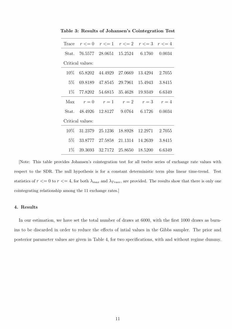
Table 3: Results of Johansen’s Cointegration Test
Trace r <= 0 r <= 1 r <= 2 r <= 3 r <= 4
Stat. 76.5577 28.0651 15.2524 6.1760 0.0034
Critical values:
10% 65.8202 44.4929 27.0669 13.4294 2.7055
5% 69.8189 47.8545 29.7961 15.4943 3.8415
1% 77.8202 54.6815 35.4628 19.9349 6.6349
Max r = 0 r = 1 r = 2 r = 3 r = 4
Stat. 48.4926 12.8127 9.0764 6.1726 0.0034
Critical values:
10% 31.2379 25.1236 18.8928 12.2971 2.7055
5% 33.8777 27.5858 21.1314 14.2639 3.8415
1% 39.3693 32.7172 25.8650 18.5200 6.6349
[Note: This table provides Johansen’s cointegration test for all twelve series of exchange rate values with
respect to the SDR. The null hypothesis is for a constant deterministic term plus linear time-trend. Test
statistics of r <= 0 to r <= 4, for both λmax and λTrace, are provided. The results show that there is only one
cointegrating relationship among the 11 exchange rates.]
4. Results
In our estimation, we have set the total number of draws at 6000, with the first 1000 draws as burn-
ins to be discarded in order to reduce the effects of intial values in the Gibbs sampler. The prior and
posterior parameter values are given in Table 4, for two specifications, with and without regime dummy.
11
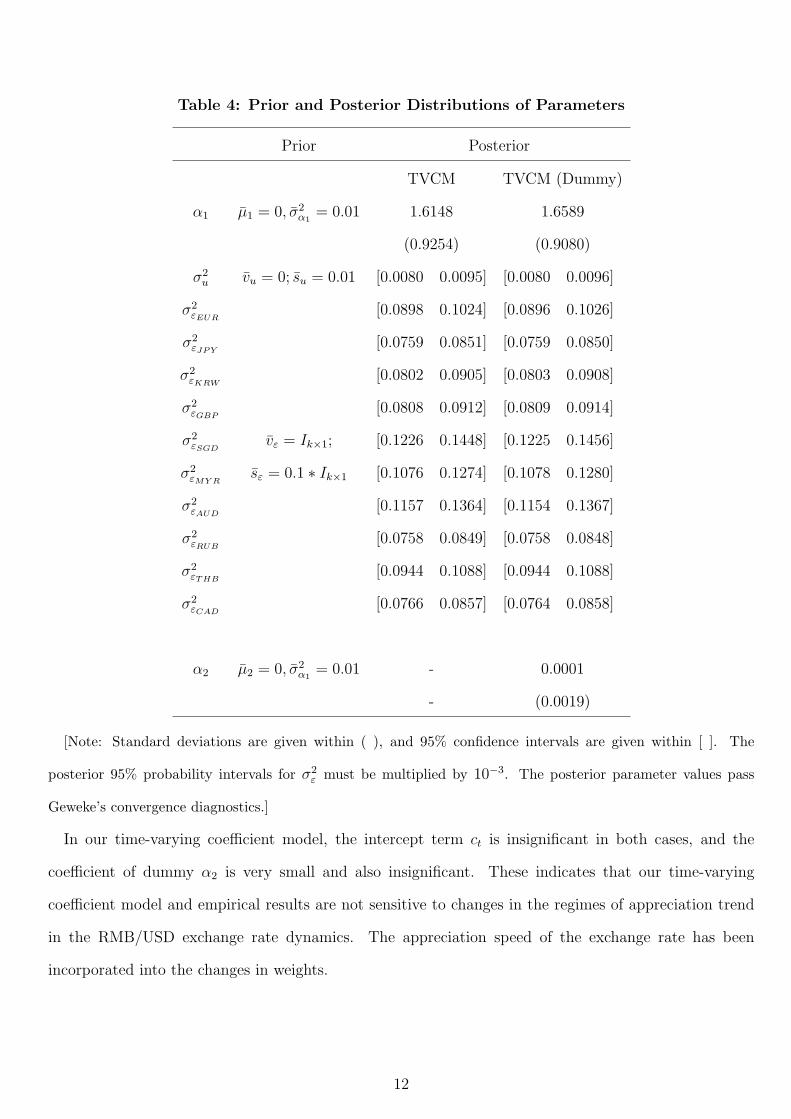
Table 4: Prior and Posterior Distributions of Parameters
Prior Posterior
TVCM TVCM (Dummy)
α1 µ̄1 = 0, σ̄2α1
= 0.01 1.6148 1.6589
(0.9254) (0.9080)
σ2u v̄u = 0; s̄u = 0.01 [0.0080 0.0095] [0.0080 0.0096]
σ2εEUR
[0.0898 0.1024] [0.0896 0.1026]
σ2εJPY
[0.0759 0.0851] [0.0759 0.0850]
σ2εKRW
[0.0802 0.0905] [0.0803 0.0908]
σ2εGBP
[0.0808 0.0912] [0.0809 0.0914]
σ2εSGD
v̄ε = Ik×1; [0.1226 0.1448] [0.1225 0.1456]
σ2εMY R
s̄ε = 0.1 ∗ Ik×1 [0.1076 0.1274] [0.1078 0.1280]
σ2εAUD
[0.1157 0.1364] [0.1154 0.1367]
σ2εRUB
[0.0758 0.0849] [0.0758 0.0848]
σ2εTHB
[0.0944 0.1088] [0.0944 0.1088]
σ2εCAD
[0.0766 0.0857] [0.0764 0.0858]
α2 µ̄2 = 0, σ̄2α1
= 0.01 - 0.0001
- (0.0019)
[Note: Standard deviations are given within ( ), and 95% confidence intervals are given within [ ]. The
posterior 95% probability intervals for σ2ε must be multiplied by 10−3. The posterior parameter values pass
Geweke’s convergence diagnostics.]
In our time-varying coefficient model, the intercept term ct is insignificant in both cases, and the
coefficient of dummy α2 is very small and also insignificant. These indicates that our time-varying
coefficient model and empirical results are not sensitive to changes in the regimes of appreciation trend
in the RMB/USD exchange rate dynamics. The appreciation speed of the exchange rate has been
incorporated into the changes in weights.
12
4.1. Estimated Weights in the RMB Currency Basket
To visualize the time-varying weights intuitively, we plot the median estimates over time along with
the 95% probability interval.
We first present in Figure 2 the time-varying weight on the US dollar. It is still dominant over other
currencies, on average accounting for 85% of the value change in RMB, which confirms the impression of
the RMB/USD dynamics given in Figure 1. There are three major periods when the weight is significantly
below one: (1) July 2005, when Chinese authorities announced the switch to the new currency regime;
(2) December 2008, when the sub-prime crisis broke out; (3) late 2010 and early 2011, when China’s
growth rate and economic indicators seemed to excel against the dismal backdrop of the world economy,
and China is again under acute pressure from the U.S. to accelerate the RMB appreciation process.
[Figure 2. Time-varying Weight of the US Dollar]
Figure 3 plots the estimated time-varying weights on five major international currencies other than the
USD in the basket, i.e. the euro (EUR), British pound (GBP), Japanese yen (JPY), Australian dollar
(AUD) and Canadian dollar (CAD), respectively. Although the first three international currencies were
announced as major currencies in the basket along with the US dollar, the weight of yen is significantly
positive only in July 2005 when the new exchange rate regime was introduced, and the weight of the
pound is once significant at the end of 2008 in the crisis, while the euro weight never turns positive
significantly. As for the other two international currencies, the weight on AUD is flat around zero during
the whole sample period, and the CAD only significantly drops to negative at the end of 2008, reflecting
its close link to the US dollar.
[Figure 3. Time-varying Weights of Five International Currencies]
Figure 4 plots weights of Asian currencies in the announced basket other than the Japanese yen. The
Korean won (KRW) is significant only around July 2005, then tends to be negative at the end of 2008, but
remains around zero. The Russian ruble (RUB) was significantly positive at the end of 2008. The other
three East Asian currencies exhibit significantly positive weights on several occasions. The Malaysia
ringgit (MYR) becomes significantly positive during the first half of 2008, then tends to be positive in
2010 and 2011, and the median weight stays positive most of the time. The Singapore dollar (SGD)
13
has large swings to the positive side in 2005 and remains for some time positive with significance in the
beginning of 2011. The Thailand baht (THB) becomes significantly positive every time the US dollar
drops significantly below one.
[Figure 4. Time-varying Weight of Asian Currencies Other than the Japanese Yen]
The above results echo the findings in Frankel and Wei (2007) and Frankel (2009) in that:
1) The RMB did relax its peg to the US dollar since July 2005, although a rigid peg was resumed
during the financial crisis, and the weight has been constantly below one with high probability, and
significantly below one during some periods.
2) Besides the relaxation of the dollar peg, there is no systematic pattern of currency weights
discovered for the claimed currency basket.
3) When the dollar weight decreases, it is not the case that the weights of the other major inter-
national currencies increase, but that the weights of some East Asian currencies increase.
While the first two points are intuitive and in line with what the market observes, the last point is not
obvious without close examination, neither is the explanation straightforward.
Concerning the significant weight of the Malaysia ringgit from a linear regression with 2005-2007 data,
Frankel and Wei (2007) suggest that a possible reason is that the Chinese government sought to preserve
its trade competitiveness against other Asian rivals. But the explanation is not fully justified in terms
of the importance of bilateral trade with Malaysia or trade competition with Malaysia, when other trade
partners, especially some other important East Asian economies, are also included in the regression. In
the normative study of Zhang, Shi and Zhang (2011) to construct optimal currency basket for China with
the policy goal of stablizing its balance of payment, they find that, although diversification is beneficial,
the bulk weight of RMB currency basket should be placed on euro and Japanese yen in addition to the
US dollar.
In what follows, we offer an explanation via a mutual regression by regressing exchang rate changes of
the Asian economies on RMB’s exchang rate variation, controlling for major international currencies.
4.2. Weights of RMB in the de Facto Currency Baskets of East Asian Economies
In a bilateral relationship between a dependent and an explanatory variables, say y and x, the regression
coefficient in a linear model always closely reflects the covariation (x′y) between the two variables. When
14
we see the puzzling phenomenon of the increasing weights of some East Asian economies in the RMB’s
value, this means, other things being equal, that the covariation between them is increasing. Then an
interesting point is to look in the opposite direction: under the new regime of RMB exchange rate, has
its influence for these East Asian economies changed? How have these East Asian economies adjusted
their currency values with respect to a more flexible RMB? This is a very sensitive question, as China is
a very important trade partner of economies in East Asia. When China changes its exchange rate policy
with respect to the US, it has a significant impact on trade relationships within the region. Thus it is
crucial for East Asian currencies to react accordingly.
To verify this hypothesis, we run a regression for equation (6) to discover the weights of international
currencies and the RMB for the Korean won. We assume that its currency basket includes the four
major international currencies, USD, EUR, JYP and GBP, plus the RMB. The reference currency is
SDR. Although RMB and USD are highly correlated, the fact that it is not a case of strict pegging after
July 2005 renders independent the variation of the RMB value with respect to the US dollar, which
enables the estimation. We run the regression also with other East Asian currencies – RUB, MYR, SGD
and THB – to elicit weights in the currency basket of each.
Figures 5 to 9 plot the results of the de facto currency baskets for these five Asian economies in turn.
Each figure presents the regression coefficients of all five weights for USD, EUR, JYP, GBP and RMB
in the basket.
We have shown in Figure 4 that the KRW and RUB actually do not often show significant weights.
In Figure 5, the result of the regression of KRW on RMB as one of the basket currencies also shows no
evident relationship between them. Though in Figure 6, the RMB does start to load positively on the
RUB at the end of the sample, i.e. in 2011.
[Figure 5. Time-varying Weights of the de Facto Currency Basket of Korea Won]
[Figure 6. Time-varying Weights of the de Facto Currency Basket of Russia Ruble]
Figure 7 shows the de facto basket weights of the Malaysia ringgit (MYR), where the RMB weight
tends to increase sharply from 2008. In Figure 8 for Singapore dollar (SGD), the RMB weight begins
to be significantly positive already in 2005 and 2006. Although it decreases somewhat in the following
15
years, it is with a high probability of being positive. Starting in 2010 it increases again with an average
of 0.5. Figure 9 shows that since 2005 the RMB weight for Thailand baht (THB) remains significantly
positive, averaging 0.3-0.4 most of the time.
[Figure 7. Time-varying Weights of the de Facto Currency Basket of Malaysia Ringgit]
[Figure 8. Time-varying Weights of the de Facto Currency Basket of Singapore Dollar]
[Figure 9. Time-varying Weights of the de Facto Currency Basket of Thailand Baht]
The above results demonstrate that some East Asian economies, whose weights tend to pick up in
the de facto RMB currency basket, have a strong tendency to increase the RMB weights in their own
currency baskets. Higher weights of the RMB in the currency baskets of these East Asian currencies
result in higher weights of Asian currencies in the de facto RMB currency basket when the US weight
drops, as the relationship is bilateral in the two way regression.
These results suggest that these East Asia economies have been placing greater weights on the RMB
systematically. On the contrary, the currency basket of RMB is more of a technical construction rather
than systematic policy operation, as we have not seen evident patterns of weights, or changes in weights,
for currencies other than the US dollar.
5. Conclusions
We employ a Bayesian method to assess the time-varying weights of China’s de facto currency basket
using daily data for February 2005 to July 2011. By including all the 11 currencies announced by the
Chinese authority in the regression, we confirm the general impression of markets and previous literature
that the US dollar still dominates other currencies in determining the value of China’s RMB, although
under the new regime of limited flexibility the weight has been below one during some periods. There
seems not yet to exist a systematic weighting scheme for the Chinese authorities, with little evidence
of increasing importance of other major international currencies. The occasionally increasing weights of
some East Asian currencies in the RMB basket can be explained largely by the greater importance of a
more flexible RMB in determining the currency values of these economies.
16
Acknowledgements
Ying Fang acknowledges financial support from the Natural Science Foundation of China (Grant No.
70971113) and Central Universities Research Fund of Xiamen University (2010221092). Linlin Niu ac-
knowledges the support from the Natural Science Foundation of China (Grant No. 70903053).
6. References
Branstetter, L. and Lardy, N. R., 2008, China’s embrace of globalization, in L. Brandt and T. G.
Rawski, Ed., China’s Great Economic Transformation, New York: Cambridge University Press.
Cai, Z., Chen, L. and Fang, Y., 2012, A new forecasting model for USD/CNY exchange rate, Studies
in Nonlinear Dynamics & Econometrics, 16(2), forthcoming.
DeJong, P. and Shephard, N., 1995. The Simulation Smoother for Time Series Models, Biometrika,
82, 339-350.
Frankel, J. A. and Wei, S., 2007, Assessing China’s exchange rate regime, Economic Policy, 22, pp.575-
627.
Frankel, J. A. and Wei, S., 2008, Estimation of de facto exchange rate regimes: synthesis of the
technique for inferring flexibility and basket weights, IMF Staff Papers, 55, 384-416.
Frankel, J. A. 2009, New Estimation of China’s Exchange Rate Regime, Pacific Economic Review,
14(3), pp.346-360.
Fidrmuc, J., 2010, “Time-varying exchange rate basket in China from 2005 to 2009”, Comparative
Economic Studies, 52(4), pp.515-529.
Ogawa, E., and Sakane M., 2006, Chinese Yuan after Chinese exchange rate system reform, China &
World Economy, 14(6), pp.39-57.
Shah, A., Zeileis, A., and Patnaik, I., 2005, “What is the new Chinese currency regime?”, Working
Paper, WU Vienna University of Economics and Business.
Zhang, Z., Shi, N., and Zhang, X., 2011, “China’s New exchange rate regime, optimal basket currency
and currency diversification”, BOFIT Discussion Paper 11/2011.
17
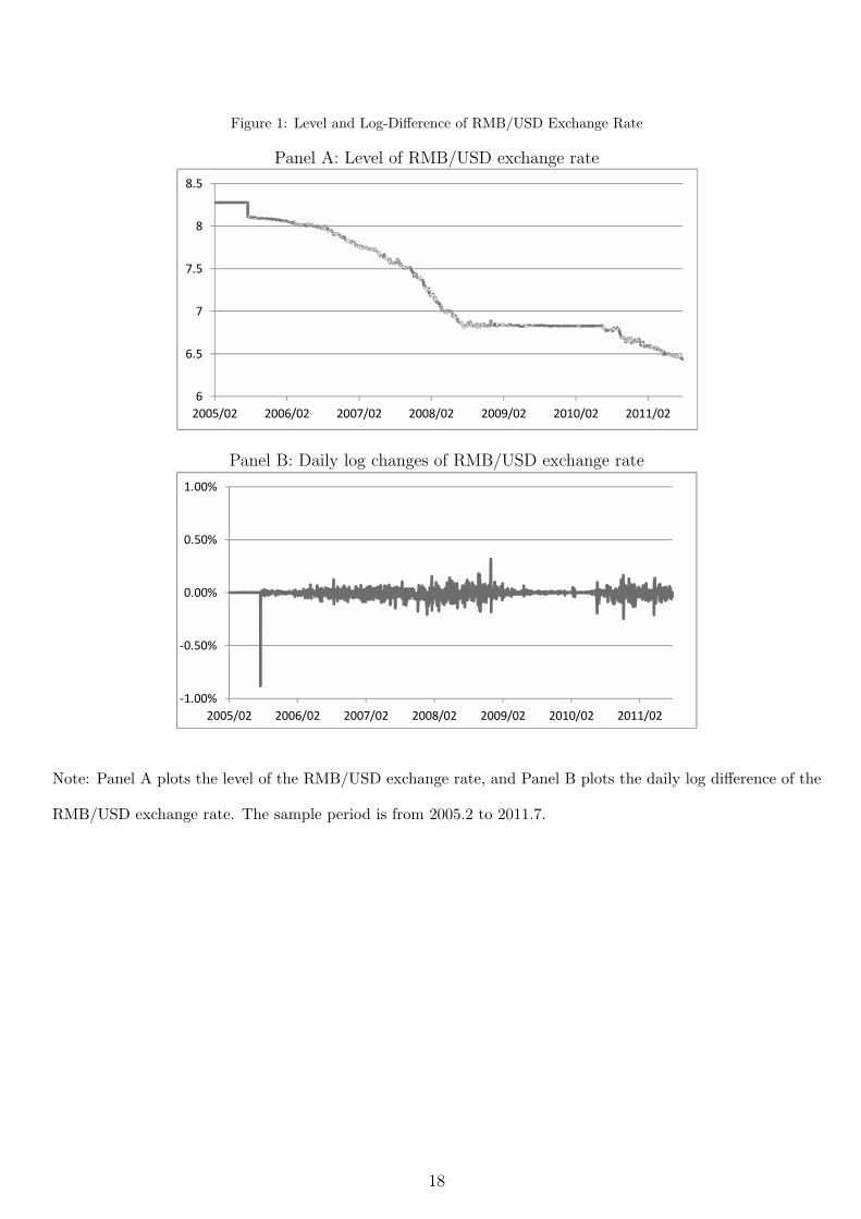
Figure 1: Level and Log-Difference of RMB/USD Exchange Rate
Panel A: Level of RMB/USD exchange rate
Panel B: Daily log changes of RMB/USD exchange rate
Note: Panel A plots the level of the RMB/USD exchange rate, and Panel B plots the daily log difference of the
RMB/USD exchange rate. The sample period is from 2005.2 to 2011.7.
18
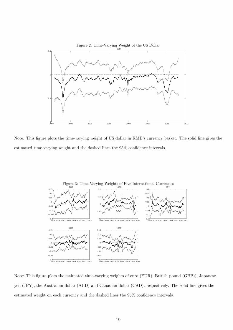
Figure 2: Time-Varying Weight of the US Dollar
2005 2006 2007 2008 2009 2010 2011 20120
0.5
1
1.5USD
Note: This figure plots the time-varying weight of US dollar in RMB’s currency basket. The solid line gives the
estimated time-varying weight and the dashed lines the 95% confidence intervals.
Figure 3: Time-Varying Weights of Five International Currencies
2005 2006 2007 2008 2009 2010 2011 2012- 0.2
- 0.15
- 0.1
- 0.05
0
0.05
0.1
0.15EUR
2005 2006 2007 2008 2009 2010 2011 2012- 0.2
- 0.1
0
0.1
0.2GBP
2005 2006 2007 2008 2009 2010 2011 2012- 0.15
- 0.1
- 0.05
0
0.05
0.1
0.15
0.2JPY
2005 2006 2007 2008 2009 2010 2011 2012- 0.2
- 0.15
- 0.1
- 0.05
0
0.05
0.1
0.15AUD
2005 2006 2007 2008 2009 2010 2011 2012- 0.2
- 0.15
- 0.1
- 0.05
0
0.05
0.1
0.15CAD
Note: This figure plots the estimated time-varying weights of euro (EUR), British pound (GBP)), Japanese
yen (JPY), the Australian dollar (AUD) and Canadian dollar (CAD), respectively. The solid line gives the
estimated weight on each currency and the dashed lines the 95% confidence intervals.
19
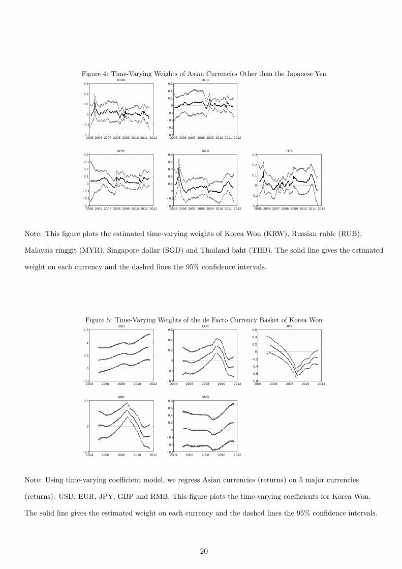
Figure 4: Time-Varying Weights of Asian Currencies Other than the Japanese Yen
2005 2006 2007 2008 2009 2010 2011 2012- 0.2
- 0.1
0
0.1
0.2
0.3KRW
2005 2006 2007 2008 2009 2010 2011 2012- 0.4
- 0.3
- 0.2
- 0.1
0
0.1
0.2
0.3RUB
2005 2006 2007 2008 2009 2010 2011 2012- 0.3
- 0.2
- 0.1
0
0.1
0.2
0.3
0.4MYR
2005 2006 2007 2008 2009 2010 2011 2012- 0.2
- 0.1
0
0.1
0.2
0.3
0.4
0.5SGD
2005 2006 2007 2008 2009 2010 2011 2012- 0.2
- 0.1
0
0.1
0.2
0.3THB
Note: This figure plots the estimated time-varying weights of Korea Won (KRW), Russian ruble (RUB),
Malaysia ringgit (MYR), Singapore dollar (SGD) and Thailand baht (THB). The solid line gives the estimated
weight on each currency and the dashed lines the 95% confidence intervals.
Figure 5: Time-Varying Weights of the de Facto Currency Basket of Korea Won
2004 2006 2008 2010 2012- 0.5
0
0.5
1
1.5USD
2004 2006 2008 2010 2012- 0.4
- 0.2
0
0.2
0.4
0.6EUR
2004 2006 2008 2010 2012- 0.8
- 0.6
- 0.4
- 0.2
0
0.2
0.4
0.6JPY
2004 2006 2008 2010 2012- 0.5
0
0.5GBP
2004 2006 2008 2010 2012- 0.6
- 0.4
- 0.2
0
0.2
0.4
0.6
0.8RMB
Note: Using time-varying coefficient model, we regress Asian currencies (returns) on 5 major currencies
(returns): USD, EUR, JPY, GBP and RMB. This figure plots the time-varying coefficients for Korea Won.
The solid line gives the estimated weight on each currency and the dashed lines the 95% confidence intervals.
20
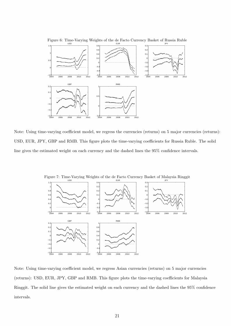
Figure 6: Time-Varying Weights of the de Facto Currency Basket of Russia Ruble
2004 2006 2008 2010 2012- 0.5
0
0.5
1
1.5USD
2004 2006 2008 2010 2012- 0.6
- 0.4
- 0.2
0
0.2
0.4
0.6
0.8EUR
2004 2006 2008 2010 2012- 0.4
- 0.3
- 0.2
- 0.1
0
0.1
0.2
0.3JPY
2004 2006 2008 2010 2012- 0.3
- 0.2
- 0.1
0
0.1
0.2GBP
2004 2006 2008 2010 2012- 0.5
0
0.5
1RMB
Note: Using time-varying coefficient model, we regress the currencies (returns) on 5 major currencies (returns):
USD, EUR, JPY, GBP and RMB. This figure plots the time-varying coefficients for Russia Ruble. The solid
line gives the estimated weight on each currency and the dashed lines the 95% confidence intervals.
Figure 7: Time-Varying Weights of the de Facto Currency Basket of Malaysia Ringgit
2004 2006 2008 2010 2012- 0.2
0
0.2
0.4
0.6
0.8
1
1.2USD
2004 2006 2008 2010 2012- 0.3
- 0.2
- 0.1
0
0.1
0.2
0.3
0.4EUR
2004 2006 2008 2010 2012- 0.4
- 0.3
- 0.2
- 0.1
0
0.1
0.2
0.3JPY
2004 2006 2008 2010 2012- 0.4
- 0.3
- 0.2
- 0.1
0
0.1
0.2
0.3GBP
2004 2006 2008 2010 2012- 0.4
- 0.2
0
0.2
0.4
0.6
0.8
1RMB
Note: Using time-varying coefficient model, we regress Asian currencies (returns) on 5 major currencies
(returns): USD, EUR, JPY, GBP and RMB. This figure plots the time-varying coefficients for Malaysia
Ringgit. The solid line gives the estimated weight on each currency and the dashed lines the 95% confidence
intervals.
21
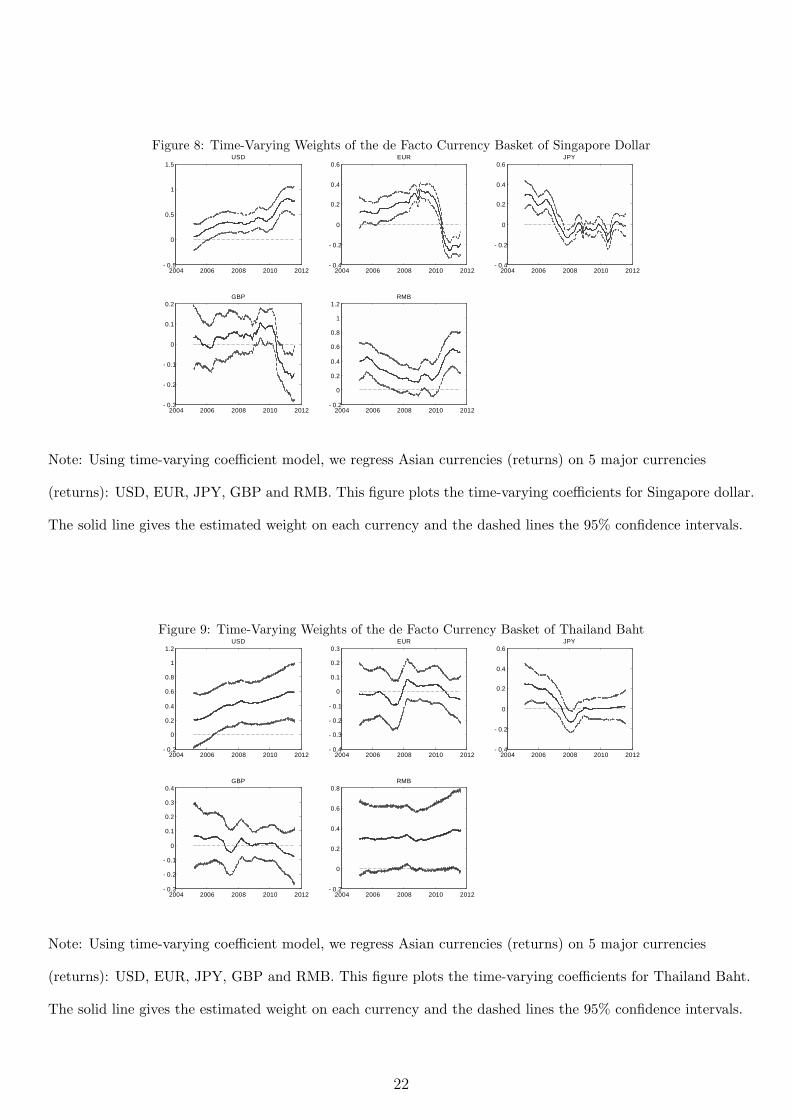
Figure 8: Time-Varying Weights of the de Facto Currency Basket of Singapore Dollar
2004 2006 2008 2010 2012- 0.5
0
0.5
1
1.5USD
2004 2006 2008 2010 2012- 0.4
- 0.2
0
0.2
0.4
0.6EUR
2004 2006 2008 2010 2012- 0.4
- 0.2
0
0.2
0.4
0.6JPY
2004 2006 2008 2010 2012- 0.3
- 0.2
- 0.1
0
0.1
0.2GBP
2004 2006 2008 2010 2012- 0.2
0
0.2
0.4
0.6
0.8
1
1.2RMB
Note: Using time-varying coefficient model, we regress Asian currencies (returns) on 5 major currencies
(returns): USD, EUR, JPY, GBP and RMB. This figure plots the time-varying coefficients for Singapore dollar.
The solid line gives the estimated weight on each currency and the dashed lines the 95% confidence intervals.
Figure 9: Time-Varying Weights of the de Facto Currency Basket of Thailand Baht
2004 2006 2008 2010 2012- 0.2
0
0.2
0.4
0.6
0.8
1
1.2USD
2004 2006 2008 2010 2012- 0.4
- 0.3
- 0.2
- 0.1
0
0.1
0.2
0.3EUR
2004 2006 2008 2010 2012- 0.4
- 0.2
0
0.2
0.4
0.6JPY
2004 2006 2008 2010 2012- 0.3
- 0.2
- 0.1
0
0.1
0.2
0.3
0.4GBP
2004 2006 2008 2010 2012- 0.2
0
0.2
0.4
0.6
0.8RMB
Note: Using time-varying coefficient model, we regress Asian currencies (returns) on 5 major currencies
(returns): USD, EUR, JPY, GBP and RMB. This figure plots the time-varying coefficients for Thailand Baht.
The solid line gives the estimated weight on each currency and the dashed lines the 95% confidence intervals.
22