Embed Size (px)
Citation preview


REVISTA DE ECONOMÍASegunda Época
Volumen 18 Número 2 Noviembre 2011
Conferencia: Problemas Fiscales y de Deuda en el Hemisferio Norte ............5Cosima BaronePhilip SuttleJulio de Brun
Understandng Unconventional Monetary Policy:A New Monetarist Approach ....................................................................43
Stephen D. Williamson
Análisis de las Calificaciones de Riesgo Soberano:El Caso Uruguayo .....................................................................................71
Fernando BorrazAlejandro FriedDiego Gianelli
La Demanda de Dinero en una Economía Dolarizada:Una Estimación para Uruguay ................................................................101
Conrado BrumElizabeth BucacosPatricia Carballo


The World at a Crossroad
The world is revealing itself as an extraordinary unstable place. Economic imbalances, wealth disparities and unwieldy finance, all contribute to the current situation bugging global financial markets. Of historical and unprecedented nature are the global expansion of debt and the central bank monetization trend of recent decades. Undoubtedly, the massive growth of debt and ballooning central bank balance sheets nurture a myriad of vulnerabilities, resulting from speculative finance and leading to boom and bust dynamics.
Nowadays, the global sentiment is shifting. Optimism on the sustainability of global recovery is dimming. And the general economic “soft-patch” talk is turning into possible “double-dip” scenario in the largest economies, while some red-hot emerging economies are sliding into “soft-patch” growth territory.
1. Major Power Shifts
I shall begin with my area of experience and tell you what I have observed from the particular angle of Wall Street and global financial markets during the last decades.
A main event, that I would like to mention here is when, on August 15, 1971, the U.S. President Richard Nixon decided to shut down the “Gold Window” and severed the Bretton Woods Agreement. As a result, “paper
ROUND TABLE ON“DEBT AND FISCAL PROBLEMS IN THE NORTH”1
COSIMA BARONE2
1 Round-table integrated by Cosima Barone, Philip Suttle and Julio de Brun and organized by the Central Bank of Uruguay during XXVI Jornadas Anuales de Economía that were held in Montevideo, on 18th and 19th of August 2011.
2 Cosima F.Barone is Chairman of FINARC S.A. – Geneva, which provides unbiased financial services to institutions and individuals worldwide.

CRISIS DE DEUDA EUROPEA6
money” became the common medium of exchange to measure “equality” and “consequences” of economic development. Paper money, not to be confused with wealth, has value on two predominant accounts: 1) because the government in power says so, and 2) because people are willing to accept it as payment. However, governments and central banks retain little control over the actions and reactions of paper money holders throughout the globe.
Fast-forward to 1975, when the global financial world was hit by a major event that no one seems to remember any more. It had the effect of a “tsunami”, which marked the beginning of a multi-decade period when global finance interests were, more and more each day, distancing them-selves from the “real” economy. On May 1st of 1975, modern finance was energized when NYSE “fixed commissions” charged on financial transactions were abandoned at the altar of “negotiated commissions”. The aim was to encourage a larger public participation in Wall Street, so that liquidity would be enhanced and risk be spread throughout all investors, institutions and individuals.
As a result, financial engineers multiplied their efforts, with intelligence and innovation, to create sophisticated financial instruments for investors. The financial industry made larger use of debt, securitization and proprietary trading. Incidentally, “High Frequency Trading” has already claimed the “flash crash” of May 6, 2010! In plain English, the message given out to the world by the 1975 shift in the NYSE commission system was that ...every American and world’s citizen had the right to own a piece of the national and global economy. The untold message, however, truly was that ...upstairs trading needed a larger trading base on which to build successfully its creative investment strategies!
Financial sophistication is not privy of major consequences. The individual investor is not in a position to effectively compete with algorithm-based financial trading systems, which remain only available to the happy few, who command a large and growing share of the overall trading volume. As a consequence, “human” traders are becoming a rarity while “supercomputers” continue to trade with each other! But, for how long? And, how big is the resulting systemic risk of modern day finance? In a nutshell, since the 1970s and under the complacent eyes of governing authorities (government, central banks and financial regulators) the bearing

REVISTA DE ECONOMÍA 7
of financial risk has consistently and systemically slipped from the hands of the global financial institutions onto the shoulders of individuals, less able to cope with it!
1971 and 1975 were also the years when the global liquidity spigots were left wide open “ad infinitum”! All subsequent events just filled the pages of a financial history book that was already in the works since August 1971.
It is important, therefore, to understand that today’s financial mess is part of a systemic debasement of the global financial system that started decades ago. Along the years and decades, capital was displaced from under the control of central banks and governments into “private” individual and institutional hands, often in foreign countries, and in the “shadow banking system”. Governments and central banks, as a result do not have adequate control of the economy and financial markets.
It is disappointing, indeed, to witness the immense lack of knowledge of leading policy makers around the globe about how the economy and finance are intimately intertwined and about the ever evolving technical intricacies of sophisticated modern finance. This ignorance inexorably leads to miscalculation of risk exposure and to systemic risk’s day of reckoning.
When this well oiled system stops working, it is the policy makers and central banks that are called to rescue the financial system. How can they rescue effectively a financial system of which they simply ignore the increasingly fast evolving sophistication? Yet, the “Sovereign State” is overtaking the “Sovereign Individual”!
2. Currency Unions and the Euro Experiment
A brief glance at history reveals that, before the U.S. Dollar’s reign as a “reserve” currency began in earnest in 1920, there have been five well defined cycles, each lasting approximately a century, when a “superpower of the world” imposed its currency supremacy over other countries: Portuguese (1450-1530), Spanish (1530-1640), Dutch (1640-1720), French (1720-1815) and British (1815-1920).

8
Currency Unions too have a long history. They tend to come and go. Currency Unions have a good chance to be successful and stand the test of time only when:
a) based on economic inter-relationships and acceptable power structures among union members, as well as between the union and other currency zones and currencies;
b) rampant arbitrage is not allowed;c) there is also a political union (i.e., in USA, USSR, UK and
Germany);d) there is a single fiscal policy;e) there is a central monetary management;f) wage and price flexibility are a “sine qua non”;g) there are clear convergence criteria; and...h) there are clear monetary convergence targets.
Ever since the fall of the Roman Empire, a dream of European unity and of a dominant European political structure has long animated the continent. After two World Wars, Europe was finally liberated from Nazism in 1945. In November 1989, with the tearing down of the Berlin Wall, the Eastern-half of the European continent was able to overcome 40 years of communism. Finally, European political division started healing. The healing process culminated with the historic milestone of May 1, 2004, when barriers created by the Cold War were finally removed.
With the accession of Bulgaria and Romania in 2007, the EUROPEAN UNION (EU) counts 27 Member States, with a total population of almost 503 million inhabitants -- 23 official languages. Despite all the agonising about whether or not it would work, the European Union has effectively created the world’s largest trade bloc stretching from the Atlantic to the borders of Russia, with a nominal GDP over €12 trillion (in 2010) -- or, approximately $16 trillion, larger than the $14.7 trillion of the United States. With 7% of the world population, the EU’s trade accounts for about 20% of global exports and imports, only second to the U.S.A.
Within this larger Community exists a separate currency union, the EUROZONE, made of 17 member states which have adopted the EURO as a common currency. The EUROZONE represents a total population of almost 332 million inhabitants, and €9.2 trillion GDP (2010).
CRISIS DE DEUDA EUROPEA

REVISTA DE ECONOMÍA 9
The adoption of the EURO was expected to lead to economic convergence, but that has not happened. The European Union failed badly by not creating first a “political union”, which would have been the “indispensable solid foundation” for the economic, monetary and fiscal bloc’s survival.
In principle, the European dream was extraordinary: nations would be combined into a single economic regime, which in turn would evolve into a single united political entity! The idea was impressively imaginative and a great gamble! The trouble is that it has not worked.
The European project was to endorse “unity” in all respects: social, political, economic and strategic including security and defense. Being “European” would have to translate into sharing a “single fate” and “common burdens”. With hindsight, Europeans only shared interests, but not a single fate! Furthermore, the European Monetary Union, fierily trumpeted at the four corners of the planet as a smashing success, is turning out already to have been a monumental failure.
To be successful, a single-currency union must involve a central or federal government, with tax and public expenditure authority, based on a “national” or “federal” GDP, also able to run significant deficits when necessary. The absurdity in the EURO currency union turns around the fact that, within the OECD, member states in the EURO union are the only governments issuing sovereign debt in a currency -- the EURO -- that they cannot print at will!
Moreover, the EU has no provisions for monetary divorce! During the decades leading to the EU and the single currency launch, the possibility was not even remotely contemplated of a member state willing to exit the single currency system. As a consequence, no institutional and legal frame-work is available to allow a member state to quit the currency union.
Recently, the EURO has come under ferocious attacks in global financial markets as the European financial, economic and sovereign debt crises moved to a new level. The cruel reality is that “debtor” nations are lending to “borrower” nations! Furthermore, the European Union and the Central Bank, even with the benevolent help of the International Monetary Fund, could fail in their efforts to contain the crises.

10
European politics are in great turmoil nowadays. At stake are not only the very survival of the EURO and the EUROZONE, but also which country within the EUROPEAN UNION is truly able to take the EU’s leadership to the next level. Emerging trends point to Germany using its economic power to reshape EU’s institutions to its own liking, while France leads the Continent on foreign and military affairs.
The notion of “unity” as in “sharing a single fate” in Europe became suddenly energized when Greece run into financial trouble. The Greek crisis unveiled the profound paradox embedded in the “European Experiment”. Being member of the EU and the EUROZONE, Greeks believed that Greece’s problems would be EU’s problems! In contrast, Berlin believed that Greek’s problems were neither Germany’s, nor EU’s problems! People in other European countries had the same reaction and felt that Greeks were foreigners.
The EURO might not be allowed to disintegrate yet, although the risk of disintegration will exist as long as European nations remain obsessed with nationalism. Individual regional powers not sharing a common vision, with fragmented military and defense policies, with no united foreign policy, with diverse economic policies and fiscal systems, could lead to disintegration of the EU bloc and common currency. If disintegration is avoided, the EU could remain an alliance of states, nothing more than a system of relationships and interests between sovereign nations. Hence, the EURO would have trouble gaining serious and predominant “reserve currency” and “store of value” status.
The whole “European Experiment” was built on a dream that economic convergence -- without mandatory fiscal convergence -- would eventually lead to a politically united Europe. Economic convergence never fully happened. Even the introduction of a common currency did not set into motion, as hoped, economic convergence within member states.
Worse, the EU is left battling every day with the many fires inflaming its member nations. And, how the EU firemen deal with the spreading fire infers a highly troublesome trend ...that EU’s member states are now able to unload risks inherent in national dwindling public finances and economic policy mistakes to the entire EU collectivity. Yet, the basic foundation of the common currency was “reliance” on the fiscal self-responsibility of each nation adhering to the EURO bloc Not only Europe is violating its
CRISIS DE DEUDA EUROPEA

REVISTA DE ECONOMÍA 11
own founding treaty -- “no country is liable for the debts of any other” -- but the European Central Bank overcame the explicit ban, within its own constitution, not to be involved in state financing. Widely considered a fatal violation of its own charter, the European Central Bank purchases member states’ sovereign debt in the secondary market and accepts sovereign securities as collateral even when they have been downgraded by rating agencies. Incidentally, the ECB bought Greek, Irish, Portuguese, Spanish and Italian sovereign bonds. As a result, the ECB holds a substantial amount of questionable sovereign debt.
The EU is quite resourceful too at times. On one hand, the EU shows commitment to established legal issues, rules and regulations, but on the other, when confronted with existential threats to the Eurozone, the UNION is able to work on the margins of its treaties -- i.e., the setup of the European Financial Stability Facility (EFSF) and subsequently the European Financial Stabilization Mechanism (EFSM) as an independent bank, headquartered in Luxembourg, which has nothing to do directly with either the EU or the EU bureaucracy. Both funds are truly at the very extreme margin of legality, based on applicable EU treaties. These bailout mechanisms do, indeed, infer how quickly the EU and the EUROZONE officials, out of necessity, sweep under the rug existing pacts if considered suicidal during crisis times.
History is in the making, as Europe tries to survive its crises with “bailout and hope” strategies! Meanwhile, the European Union has opened the door to the International Monetary Fund (IMF). This event is, indeed, a resounding precedent, which could most probably entail future consequences as this international institution could actually reign sovereign across the continent.
I believe that cracks are appearing in the sacrosanct “national sovereignty” of individual member states, even though in a “stealth” way. If a country resorting to an EU-IMF bailout is “de-facto” relinquishing its national sovereignty, and if several countries would have to face such a dramatic reality, then Brussels could strategically centralize the European sovereignty power.
Embedded into the EU-IMF bailout remains the fact that Germany, which funded the lion’s share of the EU bailout, is effectively dictating

12
the bailed-out nations’ retirement age, welfare benefits and pensions. Undoubtedly, this is the logic of a common currency, but it has important repercussions in terms of sovereignty!
In my view, it is possible that, out of necessity, a centralization process could emerge in Europe, where the people would not be asked for their opinion through risky national referendums. This scenario has every chance of becoming reality provided that European politicians design a sim-ple founding “Constitutional Treaty” to truly unite the people of Europe!
The recent convulsion spreading across global financial markets might be, indeed, putting heavy pressure on the EU to rethink and to redesign the “UNION”. Hence, threats to social stability could suddenly emerge, as mounting populist angst spreads not only in the countries being bailed out, but also in the countries doing the bailing.
3. Is an International Reserve Fund the Solution?
The world is indeed facing many economic challenges, namely the deleveraging across the West, while Japan remains stuck in deflationary doldrums, China resists a total de-peg of the Chinese Renminbi from the U.S. Dollar, and inflation picks up in emerging markets.
As the world is thorn with “liquidity” and/or “solvency” issues affecting an increasing number of countries, a call for global cooperation and coordination to address the debt problems in the United States and Europe is becoming louder by the day.
Investors, are consistently getting out of the U.S. Dollar and the EURO to literally stampede into the perceived-safety of the Japanese Yen and the Swiss Franc. Amid growing concerns over a global slowdown, Japan and Switzerland are, as a result, worried that economic problems in the U.S. and the EUROZONE are driving up the value of their currencies to “absurd” levels and hurting domestic exports.
Emerging countries, with the economy firing on all cylinders, are also attracting strong inflows of foreign capital pushing their currencies to alarming levels, threatening the vitality of their export sectors and raising inflation worries. Money flees low interest rates in the U.S., Japan
CRISIS DE DEUDA EUROPEA

REVISTA DE ECONOMÍA 13
and Europe, to reach out to plumper returns in the currency of Australia, New Zealand, Brazil, Canada, South Korea, Israel, South Africa and ...Uruguay.
“Currency Wars” began to spread across the globe as Brazil, Japan and Switzerland tried to calm currency waters, but to little avail, if any, so far. Are there viable solutions at hand?
From the ashes of the 2007-2009 crisis, the G-20 came to life as global comprehension, cooperation and coordination was deemed to be the cure to the financial and economic agony spreading across the planet. Beyond the G-20, other ideas have emerged.
The World Bank sees a multipolar global economy developing by 2025, to which emerging economies -- Brazil, China, India, Indonesia and the Russian Federation -- would contribute the largest share of total growth. Concurrently, the international monetary system “should” cease to be dominated by a single currency. The World Bank identified the U.S., the EUROZONE and China as the major growth poles driving the world to its “new order”. Based on this unfolding reality, the World Bank envisions a multicurrency system in which the U.S. Dollar, the EURO and the Chinese Renminbi, would each serve as full-fledged international currencies. However, such a system would herald a return to a fixed exchange rate arrangement between major countries providing the “reserve” currencies in a world of “free capital mobility”. Moreover, a multipolar currency system, as suggested by the World Bank, would be a daunting task requiring policy coordination and loss of national monetary policy sovereignty. As we have observed, such a system has not worked in Europe!
The IMF proposed to adopt its SDRs unit (Special Drawing Rights, created in 1969 to support the Bretton Woods fixed exchange rate system) as a global reserve currency. Hence, China seems to favour this idea. Incidentally, Madame Christine Lagarde, Managing Director of the IMF, nominated Mr. Zhu Min, the first Chinese Vice-President Special Advisor at the IMF. Are these two events related? Do they infer future intense work for a “bancor” type supranational currency (idea fathered by John Maynard Keynes)? Will a supranational currency be the solution?

14
In 2008, even the United Nations gathered global experts in view of designing reforms of the international monetary and financial system. The UN-mandated “Commission of Experts” published in September 2009 a plethora of prescriptions aimed at global coordination of monetary policy and fiscal policy, a more balanced size of the financial sector as a share of GDP, a restructuring of the financial system, the role of central banks, more balanced allocation of capital to productive use, etc. The UN too, along with the IMF and China, seems in favour of a “Global Reserve Bank” and an international “reserve” currency, not linked to the external position of any particular national economy and designed to regulate the creation of global liquidity and maintain global stability.
All represent great ideas for the future!
4. A New World standing on Values
The world is indeed at a crossroad. The world will have to choose between an ever evolving financial sector mostly disconnected from the economy made of real human beings, living in a real world, working in a real economy and deserving fair compensation for hard labour.
Some global leaders have strongly called for moral values to be put back into the management of planet Earth. It is imperative, indeed! However, their call sounds so much like “populist” political prescription during the global financial and economic crises.
Yet, people need their leaders to be visionary and to have the political courage for setting into motion progressive economic, political strategies in advance for future generations. Unfortunately, politicians only worry about the next election! In the meantime, the world of finance never sleeps! It constantly moves forward with very innovative financial engineering.
Then, how to reconcile fairness and harmony, including innovation, in this unsettled world? I strongly believe that “fair compromise” must replace “nonexistent perfection”. Politics, economics and finance have rarely, if ever, in history been in equilibrium during this most needed and essential compromising exercise. The world is facing exactly this imbalance at the present time. The imbalance is so stretched that it will take political courage and large efforts for many years, from all involved actors, in order to attain some sort of equilibrium between political, economic and financial forces for the good of people.
CRISIS DE DEUDA EUROPEA

REVISTA DE ECONOMÍA 15
Major reforms on Earth are always a product of necessity, not of mere ideological vision. I am convinced that a “new vision” will at some point emerge from the ashes of the current global crises.
However, instead of fantasizing on a “new global currency” and a “new global central bank”, both of which might take decades to develop, I believe that there is an impending need for immediate action. The citizens of world are already on the streets of their capitals wanting to work and to earn a fair price for it, to have transparent and accountable government and fiscal structures, as well as peace and harmony.
I have identified simple and straightforward actions that every government, if truly willing to work for the good of people, should consider at the national level, possibly also coordinate it internationally, without any further delay. These actions are:
Reconsider the 1. size of the government and cut down “all” excesses and “all” inefficiencies;
Simplify the 2. fiscal system, eliminate all niches -- only able to capture votes at election time -- and build a fiscal system more “just” and totally cleaned up of all complexities mostly incomprehensible to the people;
Reconsider the financial “3. derivatives” market structure in order to allow the use of derivatives only for hedging purposes of “real” transactions in the “real economy”.
Cut entirely the unnecessary 4. sophistication of financial markets across the globe.
Forbid the “5. making money with money” strategies and black pools activities (computers trading with computers) and let the people be part again of the financial market.
In other words, the financial market should stick primarily to its essential role of being the intermediary between savings and the use of these savings in the “real economy”. Banks should return to their main role of financing the “real economy”.

16
I believe that these measures, although requiring real political commitment and daunting efforts, could be discussed, negotiated and implemented in a much easier and rapid way than any other visionary international new structure at the moment. The people around the globe would understand, appreciate and support such efforts.
Admittedly, these measures might sound retrograde at the present time. But, when the machine is broken as it is now, the clock must be stopped for a while and even turned back. A dose of common sense is necessary in order to consider each economic and strategic issue in the proper perspective. Then, global economies can rebound in a stronger and sustainable way in a “NEW WORLD standing on VALUES”!
Undoubtedly, as the world economy goes through major transformative change in its growth dynamics and industrial landscape, there will be time to design appropriate mechanisms for the global governance of economies, international liquidity and reserves, and the creation of global liquidity for specific global issues (famine and water, for instance), aiming at global growth and financial stability.
The current monetary system most probably needs to be totally overhauled in order to accommodate the new realities of globally intertwined economies.
Therefore, I strongly believe that the above-mentioned first steps must imperatively be considered in each country. Indeed, a solid building requires serious architectural work at its foundations first. Otherwise, the outcome could only be a “monumental ruin” standing on multiple ruins!
Allow me to conclude this presentation with some recommendations for your beautiful country. Uruguay should particularly focus on economic strategies that would engineer internally generated growth, able to ensure solid employment perspectives to all citizens, especially to its youth. Uru-guay should reduce its dependence on foreign capital and be particularly vigilant to prevent foreign speculative capital from gaining substantial control of domestic strategic economic sectors and corporations. Political, economic and fiscal stability, are essential to attract foreign investments. But, above all foreign investors scrutinize the level of security provided by the government of Uruguay.
CRISIS DE DEUDA EUROPEA

REVISTA DE ECONOMÍA 17
ANNEX
A.1 Historical Transitions
A.2 Market capitalization

18
A.3 CURRENCy UNIONS
...TEND TO COME AND gO... ... ONLy THE U.S. DOLLAR WAS TRULy SUCCESSFUL ... ... WILL THE EURO SURVIVE THE CURRENT CRISIS?
CRISIS DE DEUDA EUROPEA

REVISTA DE ECONOMÍA 19
A.4 Is the EURO a Reserve Currency? InternationalConfidencemustbeearned!

20
A.5 EUROPE’s Milestones -- 1948 to present
CRISIS DE DEUDA EUROPEA

REVISTA DE ECONOMÍA 21
A.5 EUROPE’s Milestones -- 1948 to present ...cont.d from previous page

22
PHILIP SUTTLE1
I think I should actually congratulate Uruguay for organizing this very interesting looking conference. Also, in light of what is going on and what the previous speaker said, for showing the world that there is life after selective default. It must be said that there are many people in Europe looking at the experience of Uruguay, what happened earlier, during the past decade, and the lessons learned. Well done.
I am going to focus my comments on five areas. My comments will focus much more on shorter-term economic issues, so I think it fits very nicely with the previous presentation; they are both very different but I think they both provide interesting angles. First, I will spend some time talking about where we are, particularly how to interpret the most recent global dip. The second topic I want to spend some time on is what comes next. Third, how will the Euro crisis play out − we’ve heard some of that in the last presentation so I will not spend too much time there but I think we agree that there is a mess ahead for Europe, it is a very challenging situation. The fourth topic is actually whether S&P was right to downgrade the United States − I’ll leave my answer until I get to that, I will keep you on tenterhooks. Finally, I will conclude on how emerging economies will perform against this backdrop.
Chart 1 shows a lot of numbers, and that tells a very clear story which is that the global economy has slowed quite uniformly in recent months. In the second quarter − about three quarters of the data are in so far − it looks as though global growth has slowed to about a 2 % pace. In what we like to call “mature economies” (the OECD or what used to be high-income countries) growth is slowing to about 1 % in the first half of the year, with Japan in particular going into recession − as we’ll see in a moment − caused by the earthquake and the tsunami. What is equally noticeable, however, is that the emerging economies have held up pretty well. Through the first quarter of the year they showed some slowing which was most pronounced in East Asia, the Asia Pacific region.
1 Deputy Managing Director and Chief Economist, Institute of International Finance.
CRISIS DE DEUDA EUROPEA

* Includes IIF estimates
Chart 2 actually highlights the United States. Across the world we have seen consumer-led weakening in recent months. You can see the United States − the dark line. This axis shows the total consumer spending and the grey line at durable goods spending. You can see that, as always, durables spending had led total spending down. Obviously part of that is also consumption. A significant part of that, we think, is related to disruptions with Japan.
REVISTA DE ECONOMÍA 23
All of this just underlines the fact that global slowing has been pretty uniform and I think we are not quite at the point where we are worried about recession risks but we are clearly flirting with a period of sustained sub-par growth, with the manufacturing sector, as you’d expect, being on the weak side of average. But I think that it is quite important to know that it is not just inventories and manufacturing volatility that is giving us this slowdown: we’ve had a crossover.
Chart 1 - Interpreting the most recent global dip.

24
Chart 2 - A Consumer-led Weakening
Real Private ConsumptionPercentage 3m/3msaar (both scales)
So, when you take a step back and ask yourself what are the drivers of what I like to call a ‘mini-cycle’, I think there are five essential features which have given us this weakening. In some sense, looking at those five features is useful when thinking about where to go next. They are:
• Fiscal tightening in Mature Economies
• Monetary tightening in Emerging Markets
• Oil price surge
• Japan earthquake disruptions
• Debt crisis worries?
The first is basically fiscal tightening in the mature economies which, although I think we’ll all agree there’s still a lot of that ahead, I believe it’s important to recognize that we’ve already entered a phase of significant fiscal tightening.
CRISIS DE DEUDA EUROPEA

REVISTA DE ECONOMÍA 25
The second factor, which I think has highlighted its importance these days, is that we’ve had a significant round of monetary tightening in emerging markets, specially in countries like China and India, Brazil included as well, obviously. Both got a little concerned about inflation tensions at the end of last year and this year they have tightened their monetary policy. Maybe it is too early to expect all of that tightening to have had its effect, but certainly I think the first wave of impact has spread.
The third factor which I think we all recognize as very important is the surge in oil prices, some of it triggered by global demand but a lot of it triggered by the instability coming out of the Middle East.
The fourth factor which I think is very important but hopefully will be short-lived is the disruptions resulting from the Japanese earthquake, and that it is true specially in the auto sector. I think we’ve all been reminded once again how powerful the auto sector is.
And the fifth factor which I think is a lot more recent and therefore probably it’s premature to think that this factor is fully played out in any sense − or maybe even partially played out − are all of the worries relating to the debt crisis in Europe, the renewed worries there. Also, we can include the worries that we had in the United States.
But I think that as we look at these five factors and consider, looking ahead, how they will play out, it is fair to say that some of them are still clearly going to be with us.
What I think is important to know here is that it is pretty reasonable to expect the second half of the year to be a bit stronger. I guess one can always hope, but I think that there is more than just hope here − there are a number of factors playing out, some of which I just outlined, and, as they get a bit reversed here, they could produce a better second half readout, most notably with Japan producing a snap back, and that will help other economies. We’ve already seen in the United States, for example, some of the June/July (specially July) indicators looking better, including in the manufacturing sector, in part because of the normalization of auto production as well as auto sales. I don’t want to make too much of the auto sector, but I think it is very important to recognize that it’s been a pretty powerful influence.

26
Chart 3 - 2011 REAL gDP
Q1-Q2 averagePercent, q/q saar
Q3-Q4 averagePercent, q/q saar
And I think on top of that you have to argue that, while there are some reasons for a temporary rebound, the outlook across the major economies for the second half of the year does not actually look that bright. You can see on the right hand chart on Chart 3, the dark bars show that we’ve got a very spectacular outlook in Japan but elsewhere − the growth rates for the U.S., the Euro area (the United Kingdom, for example) − are all pretty meager, in fact in the U.S. it is expected that growth will be about 2.5 % in the second half of the year, capping off the 1 % increase in the first half. So, over the year as a whole that’s not too impressive and certainly underlines a disappointing picture.
The other point I would like to emphasize − and this is perhaps most relevant to the emerging world because this is the good news about this short-term cyclical story − is that we should see receding inflation pressures. All the signs are there, in the pipeline: whether we’re looking at oil prices, food prices or simply more general demand trends, all signs point to a moderation of inflation.
CRISIS DE DEUDA EUROPEA

REVISTA DE ECONOMÍA 27
Chart4–InflationPressuresReceding
Emerging EconomiesMature economies
How will the Euro crisis play out? I will make two basic points. One, I do not really know, but what I do know is that it’s not going to look good, it’s not going to be pretty. I think the previous speaker did a wonderful job of setting the backdrop to the Euro crisis and emphasized that this is really as much a political struggle or a political set of issues as it is an economic set of issues. That is part of the reason that I, an economist, have no idea how all those issues work and think and interact with one another. But we have to say that the precedents so far, in the last year and a half of the crisis, have not been good. As we like to say in financial markets, the politicians have not typically got out ahead of the curve; instead, they have typically responded to problems. So, I think it is reasonable to expect difficulties ahead.
I am not a monetarist, but I do like to show that if you look at the relationship between M1 growth in Europe and the leading indicator one year ahead, real GDP growth, it does seem to work quite well and it does not augur particularly well for the year ahead (Chart 5).

28
Chart 5 - Real gDP and M1 Real growthPercent change over a year ago (both scales)
In a very tough financial environment, specially in the banking sector in Europe, the ECB is likely to play a continued role as the lender of last resort, in a sense, as the de facto fiscal authority, because the ECB is really lending to the banks so that they can maintain or in some cases increase their sovereign debt holdings and if the ECB was not able to do that then banks would be forced to sell their sovereign debt holdings more aggres-sively than they have been doing then the problem would calm down a lot quicker than it is likely to do. My sense here is the Euro crisis is just going to play out as a bad story for the next year or year and a half.
CRISIS DE DEUDA EUROPEA

REVISTA DE ECONOMÍA 29
Chart 6 - The European Central Bank is the lender of last resort, for now
Lending to Monetary Financial InstitutionsPercent of banking sector assets
But I think what we’re painfully learning is that really the Euro area officials face a choice between seeing the system fragment in some fashion − I do not think we’d want to choose that option − and the other option, which is some degree of accelerated fiscal integration. We essentially think that the latter is the approach that is likely to be followed, not a preemptive measure, but the increasing widening of fiscal integration in the form of more and more centralization of debt and debt guarantees.
One more reason for that, which I think is highlighted by Chart 7, is that the credit environment at the sovereign level within Europe is really very serious. If we compare the deterioration of the credit worthiness of what we like to call the EFSF-3 (which is basically Greece, Ireland and Portugal), if you line that up against the deterioration of credit in East Asia in the Asian crisis in 1997-98, you can see that already we’re not doing so well. Frankly, a year and a half into their crisis in East Asia they’d already found a possible beginning to improve and I think we’re nowhere near that in Europe. So, I think this is really looking to be quite a serious global credit event which I think will require the choice of either euro fragmentation or, more likely, some degree of accelerated euro fiscal integration.

30
Chart 7 - Europe`s choice: EMU survival requires Fiscal Integration
Sovereign credit ratings on long-term debtAverage of Moody`s, S&P, and Fitch long-term ratings
Finally, that takes me to my fourth set of topics, which is ‘Was S&P right to downgrade the United States?’ We can all debate the validity and worth of sovereign credit worthiness indicators and sovereign ratings, but I think my answer would be, clearly, yes. Just to be fair to countries around the world, and I would refer to that point by saying that among the mature economies it’s not just the U.S. that needs to be downgraded. I think where we are fundamentally in the world is that we are seeing a significant rota-tion in creditworthiness, in a sense away from high creditworthiness in the mature economies and low creditworthiness in the emerging economies to something of a convergence.
CRISIS DE DEUDA EUROPEA

REVISTA DE ECONOMÍA 31
Chart 8 - Was S&P right to downgrade the US?
Sovereign term ratings on long-term debtAverage of Moody`s, S&P, and Fitch long-term ratings
In Chart 8 you can see the indicators. The bold line represents the mature economies, the grey line represents the emerging economies. My sense here is that in five or ten years time we are going to be converging on a sort of A+, AA type range; Uruguay will be on the way up and the United States and another set of countries will be on the way down. Frankly, this reflects all these fundamental developments that we have been looking at for the past 15-20 years. Latin America has managed to get its house in order, specially on the fiscal side, and the mature economies have done the opposite, so sovereign ratings should be expected to respond to that.

32
Chart 9 - Domestic vulnerability
Real gDP forecast for 2011Q4/Q4 (as published in IIF monthly global Economic Monitor)
One of the features of the United States is that we are struggling to grow and we are struggling to establish credible recovery. In that sense, from a sovereign creditworthiness perspective, there are problems on both sides of the calculation. The numerators of the debt ratio keep going up, debt levels keep going up because in a low-growth environment it is very hard to get the budget deficit under control – we have seen that very recently in Washington, all this rhetoric about doing something while very little gets done − and in a low-growth environment this is doubly bad because the denominator of the debt calculation just does not go anywhere. So, the numerator is going up and the denominator is flat to down. That’s very much the environment that Japan has found itself caught in recently and, I hate to say it, but the United States is looking as if it could get there as well.
CRISIS DE DEUDA EUROPEA

REVISTA DE ECONOMÍA 33
Chart 10 – External VulnerabilityFed custody holdings on behalf of foreign insitutinons
On Chart 10 we point to the external vulnerability of the United States. It is not just bad that we have domestic debt which is high and rising, but a huge amount is owed to foreigners. In fact, if you look at the left hand-side you can see that just the Fed itself has custody holdings on behalf of foreign central banks that now total about 3.5 trillion dollars, and you can see that in recent years foreign central banks − maybe the Central Bank of Uruguay would be proud of that − have been sellers of agency securities and buyers of treasury securities.
How will the emerging economies perform in this environment? I think one point to make is that it is going to remain a very challenging external environment for emerging economies. But I guess what we feel is quite important is that the domestic demand environment in many emerging economies remains quite favorable. You can see for Latin America, for example, we project around 4 % growth for this year and next − slower than 2010 but 2010 was a year of unusually strong recovery. We continue to project East Asian growth at a 7 to 8 % rate, obviously much of that led by India and China. I must confess there are probably more down-side risks in some of these numbers than up-side risks at the current time. It must be emphasized that with a very permissive monetary environment in the emerging world the prospects for domestic demand are quite good.

34
Chart 11 – How will the emerging economiesperform in this environment?
gDP growth by region
So far, what people in Uruguay, Brazil, Argentina, China, India, Turkey, what people across the emerging world need to worry about is first of all the U.S., Japan and Europe, that’s a problem. But the key challenge is having to live with global monetary policy of zero inertest rates.
Chart 12 - The key challenge
Real policy ratesPercent,deflatedbyheadlineinflation
CRISIS DE DEUDA EUROPEA

REVISTA DE ECONOMÍA 35
And I think if there is one point I would take exception with the previous speaker is that she put a lot of blame, in a sense, on the global financial system, on the global banking system, but I think you have got to worry a little bit about the policy makers and their responsibility here, in setting interest rates at these levels and keeping them there. We just heard the Feds say that they are going to keep them there until the middle of 2013… that produces a very dangerous backdrop against which I think financial markets have to operate. In a sense, you cannot think of global financial players as innocent bystanders as that would not be the case – they are certainly not innocent and they are not bystanders − but there is a system in which they have to play and operate to maximize profits, etc. And I think the picture I am showing here is a very toxic system, this is not a good environment got financial markets to operate in.
Chart 13 – Divergent credit conditions
One thing I’d like to draw your attention to is that we do a survey of the Institute’s bank members − essentially among emerging market banks − and what we are doing is asking them about credit conditions as well as demand conditions. On Chart 13, on the left had side you have a picture of whether banks are tightening or easing conditions. I think for us the good news is that in the emerging world banks are actually tightening or being quite cautious on their supply side conditions − the credit. In the left hand chart, the bars that are below 50 mean that they are tightening credit

36
conditions, above 50 it means net easing. You can see on the supply side how banking members are actually being quite cautious, but if you turn to the right-hand picture what you see is some very dramatic news on the demand side. And that just goes back to highlight what I was emphasizing earlier: that the conditions here in the emerging world are very, very buoyant in terms of domestic credit and domestic demand.
Concluding thoughts: there are five basic sets of issues to go back over. First, the global growth picture is not very good but, most important of all, global conditions remain very divergent. I would say down-side risks have intensified in recent months, although, having said that, we still think that the second half of the year will be better, so we had a bad first half and will have a slightly better second half, and then 2012 will not be that good. The European situation is bad and it is going to get worse; we are going to have a lot more local Sarkozy summits and ad hoc meetings to fix the plumbing. The fourth point would be that the U.S. is facing formidable fiscal headwinds, leaving a lot of pressure on the Fed − I would say placing excessive pressure on the Fed. I think if you go back ten years in the emerging world and I asked you all what you would like you’d all say more credit, a better environment for credit, let’s have more external finance. All I can say is be careful what you wish for.
CRISIS DE DEUDA EUROPEA

REVISTA DE ECONOMÍA 37
JULIO DE BRUN1
Es difícil atar el montón de puntas que este tema genera en un intervalo tan breve, por lo que aunque voy a dejar muchos cabos sueltos, prefiero con-centrarme en algunos aspectos, en beneficio del tiempo y la posibilidad de tener una ronda de preguntas posteriormente.
Cuando uno ve las noticias y analiza estos temas, ya sea en charlas pú-blicas como ésta o en reuniones entre amigos, tiene la tendencia a mirar los problemas de Europa como miraba los de Latinoamérica hace quin-ce o veinte años: de manera separada aun cuando estuvieran pasando simultáneamente.
En los años ochenta uno veía como Argentina, Uruguay, México o Brasil resolvían su deuda y sus problemas fiscales, de inflación y demás, como casos separados. Y de la misma manera se trataron analíticamente otros episodios posteriores.
En esta cuestión de Europa se tiende a hacer lo mismo; uno dice ‘bueno, hoy los mercados atacaron a Francia; hoy los mercados atacaron a Italia; Grecia pasó este paquete de medidas; será posible o será sostenible la deuda de Grecia; será sostenible la deuda de Portugal, de Irlanda, de España’... en fin. Uno tiende a recibir noticias, analizarlas, procesarlas y discutirlas como si estuviéramos hablando de un conjunto de países, tratándolos individual-mente. Me gustaría centrar mi charla de estos minutos en si ése es el en-foque correcto, si deberíamos estar mirando las cosas de esa manera. Creo que esto es relevante porque, además, a nivel de líderes políticos también se tiende a abordar el problema de esa forma. Ciertamente ese sería el caso correcto si estuviéramos hablando de países con ciertos vínculos comercia-les o financieros entre ellos pero esencialmente separados y en ausencia de un proyecto político de unión por detrás de ello. En ese caso sí diciéndose podría decir: ‘veamos cómo cada uno de estos países resuelve sus proble-mas fiscales y sus problemas financieros y su respectivo sistema financiero y, en definitiva, sus problemas de endeudamiento’.
1 Presidente de la Asociación de Bancos Privados del Uruguay.

38
El punto es que hoy por hoy, y repitiendo expresiones de quien me precedió en el uso de la palabra, estamos realmente en un cruce de caminos en cuanto a si debemos seguir discutiendo las cosas de esa manera. Viendo, por lo tanto, cómo distintas instituciones de cooperación financiera internacional existentes más las que se están desarrollando en la propia Europa intentan resolver estos problemas soberanos en forma aislada o si, por el contrario, se decide finalmente a nivel político tomar ésto como un único problema, relacionado no sólo con el euro como moneda sino con Europa como pro-yecto político. Yo creo que esa es la principal cuestión que se va a ventilar en los próximos meses o en los próximos años: si de esto surge un proyecto de una Europa políticamente unida y, como corolario de ello, una moneda común, o simplemente tenemos un conjunto de países con acuerdos comer-ciales, acuerdos financieros y algún régimen monetario de mayor o menor alcance, según lo que pueda ser la situación de cada uno de ellos.
Entonces, aquí surgen dos o tres cuestiones que hacen a la dificultad de este asunto. Como ya había las enumerado Cosima en su presentación, hay muchas razones por las cuales no se puede pensar que Europa sea un área monetaria común o que tenga las características de un área monetaria co-mún. En este momento, además de todos los problemas políticos ya men-cionados, Europa está en una situación con dos claras divergencias en ma-teria de tendencias de crecimiento en los últimos años: en lo que ha sido el relativamente fuerte desempeño de algunos países − el caso de Alemania, el caso de Francia − y el verdaderamente débil desempeño de otras economías fuertemente afectadas por problemas de competitividad y productividad, como el caso de Portugal, Grecia, la propia Italia y España cuando uno deja de lado todo lo que fue el fenómeno asociado a la construcción. Esas dife-rencias de productividad, esas diferencias en ciclo económico, ciertamente son puntos que en la literatura de áreas económicas se señalan en el sentido que si hay shocks tan dispares y situaciones cíclicas tan dispares no es con-veniente (o no es razonable) estar pensando en un área monetaria.
Debo precisar que respecto de estos argumentos siempre pensé que si hay un lugar en el mundo que tiene pocas de las características de área mone-taria común que se señalan en la literatura es el de los Estados Unidos de América. ¿Qué coincidencia de ciclos económicos o de convergencia de productividad puede haber entre Nebraska, Alaska, Florida, Louisiana, Ca-lifornia, Nueva York...? Entonces, en realidad, cuando uno mira los requi-sitos de una zona monetaria común, más que una cuestión normativa sobre
CRISIS DE DEUDA EUROPEA

REVISTA DE ECONOMÍA 39
qué lugares del mundo o qué regiones del mundo deberían constituir áreas monetarias y qué regiones no deberían serlo, , uno simplemente debería ver esas condiciones como el tipo de obstáculos que tiene que superar quien desea llevar adelante un proyecto político de unificación. En otros términos, para lo único que deberíamos mirar las condiciones de la constitución de un área monetaria es para preguntar: “¿Usted, en su proyecto político, está dispuesto a sobrellevar todo esto y seguir adelante más allá, pase lo que pase?. ¿O no?” Si no está dispuesto, bueno, vaya pensando en otra cosa, no se complique la vida con estos temas, pero si está dispuesto mire lo que tiene por delante.
Entonces, cuando uno mira lo que ha sido la diferencia de desempeños en Europa, que en definitiva han ido llevando a esta situación actual, en primer lugar uno observa un beneficio evidente de lo que fue para algunos países integrarse a la zona euro en términos de reducción de deuda, en términos de compresión. Un poco relacionado con esta simbiosis que ha habido en los últimos treinta años entre monedas, entre papel moneda o dinero fi-duciario y deuda de países, la mera adhesión al euro por parte de algunos países, generó una compresión de los spread de deuda más allá de lo que se justificaba por la propia dinámica de las finanzas públicas en cada país. In-dependientemente de que en un país tuviera 4, 5 o 6 por ciento del producto de déficit o tuviera un tamaño de deuda de 50, 60, 70 o 100 por ciento del producto, todos los spread en la zona euro se comprimieron simplemente por el hecho de que un país entrara al euro y por lo tanto pasara a formar parte de este club, como si la moneda común de alguna manera garantizara la solvencia de todas las deudas soberanas.
Lamentablemente, en muchos de estos países el beneficio de la reducción de spread, el efecto ingreso favorable que resultó para las economías de la reducción de spread, se tradujo en gran parte en gasto improductivo más que en contribuciones a la mejora de la productividad. Así, observamos esta trayectoria de gastos ascendentes en todos estos países, exacerbada por la crisis de fines de la década pasada y con la recesión que estos países tuvieron en los últimos años.
Entonces, hoy por hoy tenemos un problema de altos niveles de deuda y elevado déficit fiscal en varios países europeos, y uno podría dirigir una charla de estas en dos sentidos. Uno, cómo cada uno de estos paí-ses eventualmente resuelve estos problemas: ¿es sostenible la deuda de
40
Grecia?; ¿es suficiente el esfuerzo fiscal que se está haciendo?; el ta-maño de la deuda de España, ¿es preocupante o es más preocupante el nivel de su déficit fiscal?; ¿es posible que en algún momento converja hacia niveles de resultados fiscales más sostenibles en el tiempo? Uno haría un análisis de cada uno de estos países y diría: “bueno, Grecia no es sostenible; Italia capaz que sí lo es; España sí lo es, pero necesita reducir su desequilibrio fiscal”, y así por el estilo.
En esta oportunidad me gustaría plantear las cosas de otra manera, dicien-do: “¿A Carlomagno le hubiera preocupado esto? ¿George Washington, Adams, Hamilton, Jefferson, hubieran dejado que el estado de Nueva York negociara sus problemas fiscales con sus acreedores holandeses en forma independiente? ¿O hubieran considerado (como lo hicieron) el problema financiero de cada Estado como una cuestión de la Unión que querían lle-var adelante y resolverlo conjuntamente?” Ciertamente, a Carlomagno no le hubiera quitado el sueño el problema fiscal de un feudo y, ciertamente, si se hubiera procedido por parte de los fundadores de la República norte-americana en la forma que hoy actúan los gobiernos europeos con respecto a la situación fiscal de cada uno de estos países nunca se hubiera llegado a formar el Estado de la Unión. Es más, a tal punto esto es así, que Estados Unidos en su momento tuvo que encarar diferencias de problemas fiscales internos, diferencias de productividad interna, con tensiones que eventual-mente llevaron a una guerra civil, y que justamente, en la propia visión de conservar la Unión, se estuvo dispuesto a ir a una guerra para mantenerla. No quiero decir con esto que Europa termine en guerra; simplemente lo que quiero es marcar la diferencia de problemas que se tienen hoy en Europa con respecto a regiones del mundo que en su momento tuvieron un proyec-to de Unión y tomaron las medidas que fuera necesario tomar para llevar adelante ese proyecto.
Las incógnitas que a uno se le plantean hacia el futuro son si Europa va a resolver esto como un problema de la Unión Europea, en cuyo caso: i) los ajustes fiscales tendrán que producirse en cada uno de estos países, y ii) sin ser tomados como consecuencia de una imposición externa sino como el compromiso que cada uno de estos países o estas regiones tiene con la Unión, o si, alternativamente, hay que pensar que la solución de este pro-blema pone en juego la viabilidad del proyecto de Europa como Unión.
Mucho se ha hablado del efecto negativo que pueden tener en materia de crecimiento económico los ajustes fiscales en Europa. Yo creo que ha sido
CRISIS DE DEUDA EUROPEA

tan mala la calidad del gasto público en Europa en los últimos 15-20 años que buena parte de los recortes fiscales que se están planteando son excesos fiscales que, en todo caso, su eliminación es promovedora del crecimiento económico más que un shock negativo de demanda en el corto plazo. El tema fiscal esencial en Europa a largo plazo es la viabilidad de sus sistemas de pensiones y esto es un problema independiente, relacionado con la crisis actual pero que tiene que abordarse bajo cualquier escenario, independien-temente de lo que se decida con el mantenimiento de la moneda.
Las consecuencias de las reformas o de la ausencia de éstas en los países europeos en los próximos años determinará no sólo la sostenibilidad de su deuda soberana sino también si hay un freno a posibles efectos de contagio, a nivel no solamente europeo sino también a nivel mundial. . Pero lo que uno ve hoy por hoy es un discurso dual y un conjunto de medidas duales que apuntan a ambas cosas. Por un lado recordar a cada uno de los países que tienen un compromiso con la Unión Europea y por lo tanto deben llevar adelante ciertas medidas − y aquí es muy importante lo que señalaba Cosi-ma, el tema es si democráticamente cada uno de estos países está dispuesto a hacerlo: si no está dispuesto a hacerlo que no se tome la molestia de per-tenecer a la Unión, pero si quiere los beneficios de la Unión deben hacerlo. Porque en definitiva, si cada país miembro no está realmente dispuesto a tomar las medidas necesarias, entonces no vale la pena seguir insistiendo en mantener a ese país o esa región dentro de la zona del euro. O la alternativa − y algunas de las medidas que se han tomado en Europa también de alguna manera tienden un puente en ese sentido − es aceptar que eventualmente algunos de los países involucrados no puedan completar la sostenibilidad fiscal que requieren a mediano plazo, y que en ese caso los efectos hacia el resto sean lo más leves posible, en particular en lo que tiene que ver con el sistema financiero.
Quizás lo que uno debería pedir a las autoridades europeas en este trayecto es un poco más de claridad y convicción en lo que realmente quieren ha-cer. La preocupación sobre el evento de default en este contexto creo que está sobrestimada. Lo que se hizo respecto de Grecia − el anuncio respec-to del deseo de que los bancos contribuyan en un rollover de sus débitos con una especie de Brady pequeño con distintas alternativas de bonos a mediano plazo y demás − si se hubiera iniciado por el gobierno de Grecia unilateralmente, presentándolo como un anuncio frente a sus acreedores, seguramente hubiera implicado que las calificadoras de riesgo inmediata-
REVISTA DE ECONOMÍA 41

42
mente pusieran a este país en selective default hasta que se completara el proceso de aprobación por parte de los bancos de su propuesta de reestruc-tura. Como no lo hizo Grecia sino que lo hicieron las autoridades europeas, incluso como mecanismo de presión frente a los distintos bancos, esto se viste de “voluntariedad” y por lo tanto por ahora las calificadoras no han dicho nada, aunque lo que se hizo a ese respecto es exactamente lo mismo (aunque formalmente diferente debido a quien lo anuncia) que lo que hizo Uruguay en marzo del 2003 cuando inició su proceso de diálogo con sus acreedores. Entonces el selective default ya está planteado y el problema de esta falta de convicción es que se ha planteado un selective default que lo único que hace a largo plazo es mantener la expectativa de deuda de Grecia estable, si sale todo bien, en 150 por ciento del producto. O sea, hacer todo este esfuerzo para no resolver el problema de la deuda parece en todo caso un desperdicio.
La misma contradicción y dudas aparecen con los anuncios del Banco Cen-tral Europeo respecto de su compra de bonos soberanos en el mercado so-berano. Más allá de todos los problemas estatutarios que pueda tener para hacerlo, el tema es que si se ha decidido que el Banco Central Europeo va salir a comprar deuda soberana en los mercados los recursos disponibles deberían concentrarse en comprar la que está sufriendo en el momento más ataques especulativos, como la de Italia, resultando incomprensible que salga (como salió) a comprar deuda de Portugal o de Irlanda cuando ya el problema de deuda de esos países estaba incorporado en los mercados y por lo tanto lo que hiciera el Banco Central a ese respecto era poco efectivo.
En fin, repitiendo lo que decía hasta este momento yo creo que en los próxi-mos meses, más que en el próximo año, vamos a estar viendo cuál es el fu-turo de Europa, si sigue siendo una Unión o simplemente un conglomerado de países que funciona en forma más o menos en coordinada.
CRISIS DE DEUDA EUROPEA

UNDERSTANDINg UNCONVENTIONALMONETARy POLICy:
A NEW MONETARIST APPROACH
STEPHEN D. WILLIAMSON1
This version: October 2011
ABSTRACT:
This paper focuses on Federal Reserve policy in the United States after the financial crisis. Three key interventions - QE1, QE2, and forward guidance - are reviewed, and a model is outlined that can be used to help understand some of the consequences of the financial crisis, and the policy responses to the crisis. Liquidity traps play an important role in the analysis, and it is shown how the financial crisis led to an unconventional liquidity shortage, requiring an unconventional policy response.
Keywords: Money, microfoundations, monetarism, monetary policy.
JELClassifications: E40, E50
INTRODUCTION
Before the financial crisis in 2008-09 the academic economics profession perhaps seemed a well-ordered place. Economists were going about our business writing and publishing papers, debating economic issues at conferences and in the seminar room, and working with policymakers in an attempt to make the world a better place. There were disagreements of course, and sometimes those disagreements were heated, but the system seemed to be working. Mostly, good ideas appeared to be rising to the top, and academia’s structure of peer review and incentives, though of course imperfect, seemed to be working to advance economic science.
Revista de Economía - Segunda Epoca Vol. 18 Nº 2 - Banco Central del Uruguay - Noviembre 2011
1 This paper was prepared for the Banco Central del Uruguay. 2 Washington University in St. Louis and Federal Reserve Banks of Richmond and St. Louis.

44
Since the financial crisis, the world appears to have changed, though maybe we are just seeing pieces of that world that we were unaware of. People who want to assign blame for the financial crisis have targeted economists, and macroeconomists in particular, with accusations of neglect, if not corruption. Within the profession, some economists have criticized particular economic research programs as being out of touch. Krugman (2009), for example, feels that much of the mainstream developments in macroeconomics and financial economics of the last 40 years are useless and should be relegated to the trash heap. Caballero (2011) argues that macroeconomic research has been too focussed on minor perturbations of the neoclassical growth model, and that there should be more experimentation in terms of research paths. A common complaint seems to be that there has been a neglect of the study of the financial sector and its role in aggregate economic activity.
Some macroeconomic researchers may indeed have been guilty of ignoring the details of financial arrangements in their work. For example, the researchers whose work appears in Kehoe and Prescott (2007) seem dismissive of the role of monetary and financial factors in depressive economic episodes. Also Woodford (2003), an influential handbook for monetary policy, focusses exclusively on the role of monetary policy in mitigating the frictions resulting from sticky prices, while ignoring monetary exchange and financial frictions. However, plenty of rigorous and well-respected research has been conducted over the last 40 years or more that addresses the role of private information and limited commitment in financial contracts and incentive contracts, examines the functions of financial intermediaries, highlights the role of assets in exchange, and integrates these ideas in macroeconomic frameworks that are amenable to policy analysis. Indeed, we do not have to dig deeply or look far afield to find top quality macroeconomic research on imperfect financial markets and to observe macroeconomists thinking outside the box.
In Williamson and Wright (2010, 2011), Randall Wright and I discuss the details of what we call “New Monetarist Economics,” which is the area of macroeconomic research in which we work. We think of this research program as having two branches, one dealing with monetary economics, and the other with financial intermediation and banking, though in a sense our view is that this is all financial economics - a unified whole. Key contributions in the monetary economics research program are Kareken
STEPHEN D. WILLIAMSON

REVISTA DE ECONOMÍA 45
and Wallace (1980), Kiyotaki and Wright (1989), and Lagos and Wright (2005), and key early contributions in the financial intermediation research program were Diamond and Dybvig (1983), Diamond (1984), Williamson (1986, 1987), and Bernanke and Gertler (1989), building on even earlier developments in information economics.
The key New Monetarist ideas are the following:
1. To understand how financial factors are important for aggregate economic activity, we need to delve into the particulars of private information and limited commitment frictions. Private information and limited commitment are at the foundation of the role for monetary exchange, and they are also key to understanding financial contracts, financial intermediation, and the financial propagation of macroeconomic shocks.
2. To analyze monetary policy requires that we construct models that explain how and why central bank liabilities and other assets are used in exchange, and to think carefully about how the central bank functions as a financial intermediary. Monetary policy works in part because of special advantages that a central bank has in intermediating assets - principally coming from monopolies on the issue of hand-to-hand currency and on payments systems arrangements among private financial institutions.
3. Attempting to classify some subset of assets as “money” is a futile exercise. We are interested in liquidity - broadly, some notion of how assets are used in exchange (retail exchange, wholesale exchange, exchange among financial institutions). Liquidity comes in many different forms. Some liquidity is supplied by the government, some by the private sector, and some assets are liquid in some circumstances but illiquid in others. In some transactions, for example the purchase of food from a street vendor, currency is the only object accepted in exchange, i.e. currency is highly liquid in this circumstance, but other assets are highly illiquid. However, in a large-value transaction involving financial institutions such as Bank of America and JP Morgan Chase, currency is highly illiquid while other assets such as US government Treasury bills and deposits with the Federal Reserve System (reserves) are highly liquid.
These three ideas set us apart, from Old Monetarists and New Keynesians in particular. Milton Friedman and the Old Monetarists thought

46
it important to categorize some assets as “money” and other assets as “not-money,” and they did not appear very concerned with the role of financial intermediaries in the economy, other than as suppliers of “money.” For New Keynesians, monetary and financial frictions are thought to be of minor importance in conducting monetary policy, though that idea may be changing (see for example Curdia and Woodford 2010) in response to the financial crisis.
In this paper, I use a particular New Monetarist model to help make sense of some features of the financial crisis, as well as to evaluate some of the policy interventions undertaken by the Federal Reserve System in the United States after the financial crisis. I will include only an outline of the specific model used here, and refer readers to Williamson (2011) for the details.
One key feature that our model has, which is crucial for understanding some features of the financial crisis, is a distinction between different types of liquid assets. In the model, currency is a liquid asset which is necessary to engage in particular kinds of retail transactions. However, intermediated loans and government bonds - interest-bearing assets - are also important liquid assets that are used in other types of transactions. In the model, when the central bank conducts a one-time open market operation, this can act in an unconventional way. If interest-bearing assets are scarce - where scarcity is defined in a precise way in the model - then a one-time open market purchase of interest-bearing assets by the central bank will lower the real interest rate permanently. This is an illiquidity effect, in that the open market purchase essentially makes interest-bearing assets more scarce. Typically, we would think of such an open market operation as an injection of liquidity, but in this instance it actually reduces liquidity by reducing the quantity of interest-bearing assets used in transactions.
The Federal Reserve System had been granted the power by Congress to pay interest on reserve accounts at the Fed, prior to the financial crisis. Beginning in October 2008, the Fed began paying interest on reserves at 0.25%, and that policy continues to the present date. Further, since the fall of 2008 when the Fed began to intervene in financial markets in a dramatic way, the quantity of excess reserves held by financial institutions in the United States has been very large. In such an environment, monetary policy works in a quite different way than in pre-financial crisis times. Under
STEPHEN D. WILLIAMSON
current conditions, an extra unit of reserves in the financial system will be held overnight by financial institutions, and will have no marginal value in financial transactions during the day. Thus, if the Fed exchanges reserves for short-term government debt, that will be irrelevant, i.e. traditional central bank actions will have no effect. This does not mean, however, that there are no actions the Fed can take that will matter. Indeed, if the Fed changes the interest rate on reserves, then that essentially has the same effect as an open market purchase of short-term government securities would have had in the pre-financial crisis period.
The financial crisis is sometimes viewed as a puzzling event, which conventional economic theory cannot successfully confront. However, there is actually plenty of off-the-shelf economic theory that can be used to make sense of what we observed during the financial crisis. In particular, the model in Williamson (2011), which is used in this paper, uses financial intermediation theory developed primarily in the 1980s, by Townsend (1978), Diamond (1984), and Williamson (1986, 1987), and by Diamond and Dybvig (1983). It also makes use of monetary theory developed over the last 40 years or so. The costly state verification model of Townsend (1978) which gives rise to optimal debt contracts and can be used as an element in financial intermediary structures, is particular useful, as critical components of the financial crisis were non-contingent contracts, default, and the costs of bankruptcy. In this paper, we show how aggregate shocks to asset returns, risk, and the costs of bankruptcy can reproduce some key observations related to the financial crisis, in particular increases in interest rate spreads, declines in aggregate lending, and reductions in safe rates of interest.
These aggregate shocks work to explain features of the financial crisis, and also show how the scarcity of interest-bearing assets plays an important role in the financial crisis. Prior to the financial crisis, asset-backed securities played a key role in providing apparently safe liquidity in financial exchange. However, perceptions about the safety of those securities changed during the crisis so that, effectively, the private sector’s capacity for producing safe liquid assets for financial exchange declined dramatically. This type of liquidity shortage is very different from the liquidity shortages that occurred during the Great Depression in the United States, or earlier, during the banking panics of the National Banking era (1863-1913). The Great Depression and National Banking era panics were
REVISTA DE ECONOMÍA 47

48
essentially currency shortages - a very different kind of liquidity scarcity. A currency shortage can be cured through standard open market purchases of interest-bearing assets, but such central bank actions will only aggravate the liquidity scarcity that existed during the financial crisis.
Once the Fed had lowered the interest rate on reserves to 0.25% in October 2008, there were essentially no conventional options open to the central bank to ease financial conditions in the United States. In this paper I will focus on three unconventional monetary policy interventions carried out by the Fed. The first two interventions are both typically referred to as “quantitative easing.” Quantitative easing is a misnomer, first, as “quantitative” suggests that what makes this type of intervention differs by its quantitative nature, i.e. that asset quantities on the Fed’s balance sheet are being manipulated. Of course, any action by a central bank, other than the setting of administered interest rates (the central bank’s lending and deposit rates) involves quantities. In normal times, for example, most central banks intervene by targeting some overnight interest rate, and achieving that target by buying and selling quantities of assets. Second, as we will see in the paper, quantitative easing may not be easing anything.
The particular quantitative easing programs that the Fed engaged in are typically called “QE1” and “QE2.” QE1 was a program of purchases of mortgage backed securities and agency securities by the Fed, while QE2 involved purchases of long-maturity federal government bonds (Treasury debt). These purchases were fundamentally different, as the first involved the indirect purchases of private assets, while the second was closely related to conventional open market operations with the only difference being that the asset purchases were long-maturity rather than short-maturity. In any case, the argument made in the paper is that there are conditions under which neither QE1 nor QE2 would have matters for any quantities or prices. It is possible that QE1 mattered, but this would only happen if the Fed were buying private assets on better terms than the private sector was offering. In that case QE1 would have altered the allocation of credit, and would have caused a redistribution of wealth.
A third unconventional intervention is “forward guidance.” In recent years, the Fed has been somewhat more forthcoming in its policy statements concerning the future path of monetary policy, though typically the FOMC (Federal Open Market Committee) policy statement has supplied only vague
STEPHEN D. WILLIAMSON

REVISTA DE ECONOMÍA 49
information, and that information would usually refer to potential policy decisions at the next FOMC meeting (about 6 weeks in the future). From the fall of 2008 until August 2011, forward guidance took the form of “extended period” language concerning the path of the policy rate in the future. For example, in the June 22, 2011 FOMC policy statement, the committee states that they continue “... to anticipate that economic conditions--including low rates of resource utilization and a subdued outlook for inflation over the medium run--are likely to warrant exceptionally low levels for the federal funds rate for an extended period.” In its August 9, 2011 policy statement, the FOMC got much more explicit in stating that it “... currently anticipates that economic conditions--including low rates of resource utilization and a subdued outlook for inflation over the medium run--are likely to warrant exceptionally low levels for the federal funds rate at least through mid-2013.” This is a very important change, as it essentially commits the Fed to a specific policy for a period of about 2 years.
This paper will first outline some recent monetary policy interventions, focusing on the United States and the US Federal Reserve System. Following that is a brief overview of a New Monetarist model, constructed in Williamson (2011). Following that, the objective is to show how that model can be used to organize our thinking about the financial crisis, and about conventional and unconventional monetary policy responses to the crisis.
Background: Federal Reserve Balance Sheet Developments, Three Key Unconventional Interventions, and the Mechanics of Monetary Policy
Tables 1 and 2 show a summary of the Federal Reserve System’s assets and liabilities, at two different dates: January 2008 (pre-financial crisis) and August 2011. In Table 1, in January 2008 the liabilities of the Fed were structured much like they were at any date before the financial crisis. Currency was financing most of the central bank’s asset portfolio, while financial institutions held a small quantity of reserves so as to satisfy reserve requirements. Indeed, reserves were small in January 2008 mainly because these financial institutions had found clever ways (such as sweep accounts) to circumvent reserve requirements. In January 2008, the US Treasury (the fiscal authority in the US federal government) maintained deposit accounts with the Fed, but at that time the balances in those accounts were small, in part to aid the Fed in monetary control.

50
As of August 2011, in Table 1, the Fed’s liability structure had changed dramatically from the earlier period, with reserves accounting for the majority of Fed liabilities. Though the August 2011 data do not show it, Treasury account balances with the Fed have been substantial since the onset of the financial crisis - sometimes in excess of $300 billion - and have been highly volatile.
Table 1: Federal Reserve Liabilities ($billions)
Source: Federal Reserve Bulletin
On the asset side of the Fed’s balance sheet, in Table 2, the Fed’s assets in January 2008 consisted mainly of US government debt, both short-term (Treasury bills or T-bills) and long-term (Treasury bonds or T-bonds). T-bills were used in day-to-day open market operations (often involving repurchase agreements) conducted by the Fed, and T-bonds were typically rolled over as they matured, but were not bought and sold on a daily basis.
As of August 2011, in Table 2, the average maturity of the Fed’s assets had lengthened considerably from what it was prior to the financial crisis. In August 2011, the Fed held almost no T-bills, and had expanded its holdings of T-bonds considerably. Further, in August 2011 the Fed held about $1 trillion in assets that were essentially backed by private mortgage debt (and implicitly guaranteed by the federal government). In August 2001 the Fed held almost $900 billion in mortgage-backed securities issued by the government-sponsored enterprises or GSEs (actually now under government conservatorship): FNMA (or Fannie Mae) and FHLMC (or Freddie Mac). The agency securities on the Fed’s balance sheet are the liabilities of these two GSEs.
STEPHEN D. WILLIAMSON
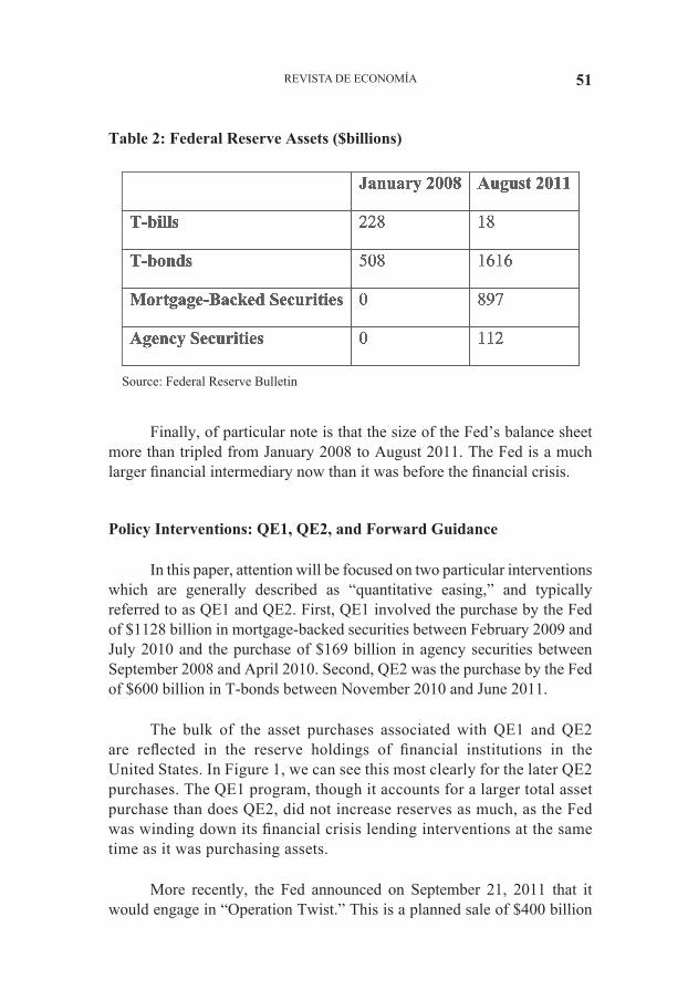
REVISTA DE ECONOMÍA 51
Table 2: Federal Reserve Assets ($billions)
Source: Federal Reserve Bulletin
Finally, of particular note is that the size of the Fed’s balance sheet more than tripled from January 2008 to August 2011. The Fed is a much larger financial intermediary now than it was before the financial crisis.
Policy Interventions: QE1, QE2, and Forward guidance
In this paper, attention will be focused on two particular interventions which are generally described as “quantitative easing,” and typically referred to as QE1 and QE2. First, QE1 involved the purchase by the Fed of $1128 billion in mortgage-backed securities between February 2009 and July 2010 and the purchase of $169 billion in agency securities between September 2008 and April 2010. Second, QE2 was the purchase by the Fed of $600 billion in T-bonds between November 2010 and June 2011.
The bulk of the asset purchases associated with QE1 and QE2 are reflected in the reserve holdings of financial institutions in the United States. In Figure 1, we can see this most clearly for the later QE2 purchases. The QE1 program, though it accounts for a larger total asset purchase than does QE2, did not increase reserves as much, as the Fed was winding down its financial crisis lending interventions at the same time as it was purchasing assets.
More recently, the Fed announced on September 21, 2011 that it would engage in “Operation Twist.” This is a planned sale of $400 billion

52
in T-bonds with remaining maturities of 3 years and less, in exchange for T-bonds with maturities of 6 to 30 years. The intervention will take place between September 2011 and June 2012. The result of operation twist will be to lengthen the average maturity of assets held by the Fed. While this may appear to be different from either QE1 or QE2, will show that, under current circumstances, Operation Twist is actually qualitatively identical to QE2.
Forward guidance, as discussed in the Introduction, involves statements by the central bank about the future course of policy. Prior to the financial crisis, Fed policy decisions concerned the setting of a target rate for the overnight fed funds rate, and communication with the public had evolved to the point where the FOMC policy statement would include some language which would signal the likely future path of the policy rate, and what that path might depend on. After the financial crisis, the Fed began to make more explicit statements about the future path for the policy rate, to the point where, in August 2011, the Fed essentially fixed the target policy rate for about two years.
How Does Fed Policy Work? Pre-Crisis and Post-Crisis
Most central bank intervention occurs roughly in the following way. If we focus just on overnight financial markets, the central bank lends to financial institutions overnight at a central bank lending rate, financial institutions can deposit funds (reserves) with the central bank overnight at a central bank deposit rate, and financial institutions can lend among themselves at a market overnight rate. There are basically three procedures that central banks typically exercise monetary control in the very short run. First, through open market operations, a central bank can intervene so as to target the overnight rate within bounds determined by the central bank lending rate (the upper bound) and the central bank deposit rate (the lower bound). This is a channel system, whereby the channel determined by the central bank lending and deposit rates “channels” the overnight rate. The Bank of Canada, for example, conforms to a channel system, and Figure 2 shows a forty-day period prior to early July 2011, illustrating the paths followed by the central bank lending rate, the central bank deposit rate, and the overnight market rate. In this case, the overnight rate was targeted at 1% over that period, and the Bank of Canada’s deposit and lending rates were set, respectively, at 0.75% and 1.25%. Further, note that the Bank of Canada
STEPHEN D. WILLIAMSON

REVISTA DE ECONOMÍA 53
managed, over this period, to conduct open market operations in such a way that there was little variability in the deviation of the overnight rate from the target. To accomplish this, the Bank needed to intervene so that funds were sufficiently tight in the system, with essentially zero reserves (deposits with the central bank) held overnight. As well, there needed to be sufficient availability of funds in the overnight market so that financial institutions did not want to borrow from the central bank at the lending rate. Under the Bank of Canada’s channel system, the overnight market rate essentially determines all short-term interest rates in Canadian financial markets.
A second way to control short-term nominal interest rates is under a regime such as what exists currently in the United States. In October 2008, the Fed announced that it would begin paying interest on reserve balances and, since December 2008, the fed funds rate (the overnight market rate) has been targeted at 0-0.25%, with the Fed paying interest on reserves at 0.25%. As we see in Figure 1, the Fed had a large and increasing stock of reserve liabilities over this period. Under these circumstances, one would expect the fed funds rate to be 0.25% over the entire period. As in the Bank of Canada’s channel system, the central bank’s deposit rate should bound the overnight rate from below. In Figure 3, this is clearly not the case, as the fed funds rate has typically been significantly less than the 0.25%. However, it is nevertheless true that the interest rate paid on reserves currently determines all short-term interest rates. This is because the GSEs, who hold reserve accounts with the Fed, do not receive interest on the balances in those accounts, and there is some lack of arbitrage.2 If the interest rate on reserves rises, we would expect the fed funds rate to rise with it.
A third alternative is for a central bank to control short-term market nominal interest rates by making the central bank lending rate the key policy rate. To do this, the central bank could essentially offer overnight loans at a particular interest rate, and then satisfy the demand for loans forthcoming at that rate. The central bank lending rate would then determine the overnight rate. The European Central Bank (ECB) operates somewhat like this through its refinancing operations, though it does not typically intervene daily to peg an overnight rate at the central bank lending rate.
2 The reasons for this lack of arbitrage appear to be something of a puzzle.

54
In conclusion, there are three ways for a central bank to influence short-term nominal interest rates, all working through the overnight market on which financial institutions trade. First, the central bank can intervene through open market operations to target the overnight rate such that it lies between the central bank’s lending rate and the central bank’s deposit rate. Second, the central bank can operate so that there is a positive quantity of central bank deposits (in excess of reserve requirements, if those exist) held overnight, in which case the central bank deposit rate determines the overnight rate. Third, the central bank could set a lending rate, and offer to satisfy all of the forthcoming demand at that rate and, further, set the rate in such a way that forthcoming demand is strictly positive. In this case, the central bank’s lending rate determines the overnight rate.
Currently, the Fed operates according to the second regime. The financial system is awash in reserves, and the interest rate on reserves (the deposit rate at the central bank) is the key policy rate. In later sections we will explore how monetary policy works under these conditions.
A New Monetarist Model
This section contains an outline of the model. For more details readers should consult Williamson (2011). The basic structure of the model is similar to Rocheteau and Wright (2005), which in turn is derived from Lagos and Wright (2005). There is an infinite horizon with time indexed by t=0,1,2,3,..., with each period having two subperiods. We will refer to the first subperiod as the decentralized market or DM, and the second as the centralized market or CM. The population consists of three types of economic agents. First, there is a continuum of buyers, with unit mass, each of whom has preferences
Here, 0 < β < 1, H1 denotes the difference between labor supply and consumption in the CM, x1 is consumption in the DM, and u(∙) is a strictly increasing, strictly concave, and twice continuously differentiable function with u (0) = 0, u’(0) = ∞ , u’(∞) = 0, – x[u’’(x) / u’(x)] < 1, for all x > 0, and with the property that there exists some x > 0 such that u (x) – x = 0. Define x* by u’ (x*) = 1. Second, there is also a continuum of sellers, with unit mass, each of whom has preferences
STEPHEN D. WILLIAMSON

REVISTA DE ECONOMÍA 55
where ht denotes labor supply in the DM and Xt is consumption in the CM. When a buyer or seller can produce (the buyer in the CM, the seller in the DM), one unit of labor input produces one unit of the perishable consumption good.
Finally, the third group of agents are entrepreneurs. In each CM, a mass of these agents is born, and they live until the next CM. An entrepreneur has an indivisible investment project with payoff w and distribution F(w), and payoffs are independent across entrepreneurs. For an individual entrepreneur, the realized payoff w is private information, but another agent can incur a verification cost γ to observe w. Entrepreneurs differ according to their observable verification cost, and G(γ) describes the distribution of verification costs across entrepreneurs. Entrepreneurs do not consume in the CM when they are born, but consume in the subsequent CM, and are risk-neutral. Since he or she has no endowment, an entrepreneur must borrow when he or she is born in order to fund his or her investment project, which is a necessary condition to consume in the next CM. This costly state verification structure is very similar to what is built into the model in Williamson (1987).
In the decentralized market, each buyer is matched at random with a seller, while in the CM everyone is in the same location. In addition to the costly-state-verification information friction that will operate in the loan market, there are elements of imperfect information in the model that inhibit other types of lending. In the DM, sellers do not know the histories (i.e. relevant credit records) of buyers, which makes credit arrangements infeasible in DM meetings between buyers and sellers. Further, market participants in the CM can only observe prices.
In the model, there are three basic assets. First, there are loans to entrepreneurs. As is detailed in Williamson (1987, 2011), costly state verification, under some restrictions, implies that intermediated debt contracts with entrepreneurs are optimal, with perfectly-diversified delegated-monitoring financial intermediaries that hold portfolios of loans to entrepreneurs. For convenience, call these financial intermediaries banks. A loan to an entrepreneur with verification cost γ
56
will in equilibrium pay a gross real loan interest rate R(γ), and R(γ) will in general reflect a default premium that is increasing in γ . In equilibrium, the expected payoff to a bank from a loan to any entrepreneur will be r, the gross market real interest rate.
Further, some entrepreneurs will receive loans in equilibrium, while others do not. There is some critical value γ* for the verification cost, such that some entrepreneurs with γ ≤ γ* receive a loan, while those with γ > γ* do not. The gross real interest rate r is an endogenous variable. If r is higher, then this will imply that the cutoff γ* is smaller, so that there is less lending. We can then write the aggregate loan quantity as L= L (r), where L(∙) is a decreasing function.
The other two assets are liabilities of the consolidated government (fiscal authority and central bank) - currency and one-period nominal government bonds. Let Mt denote the stock of money in period t, which trades at Øt price in the CM, and Bt the stock of one-period nominal government bonds, each of which sells in the period-t CM for one unit of money, and pays off q units of money in the next CM in equilibrium. Banks will be indifferent between government bonds and loans to entrepreneurs in
equilibrium, so in equilibrium we will have r = .
In the DM, in fraction ρ of meetings - non-monitored meetings - between buyers and sellers, the information technology is not available to trade loans, government bonds (account balances with the fiscal authority), or the liabilities of intermediaries holding these objects as assets. Currency is the only asset that is tradeable in non-monitored meetings. However, in fraction 1 – ρ of meetings - monitored meetings - buyers and sellers have access to an information technology that allows them to exchange claims on entrepreneurs, bonds, currency, or claims to a portfolio of those assets. In all DM meetings, goods produced by the seller can be acquired by the buyer only through an exchange of assets. For convenience, we assume that the buyer makes a take-it-or-leave-it offer to the seller.
A bank in this model has a role to play in efficiently allocating liquidity to its best uses. Effectively, in the model there are two types of liquidity: currency on the one hand, and loans and government bonds - interest-bearing assets - on the other. In non-monitored DM meetings where only currency is accepted, loans and government bonds, or claims to them,
STEPHEN D. WILLIAMSON

REVISTA DE ECONOMÍA 57
are useless. However, in monitored DM meetings where interest-bearing assets are accepted, it would be a poor choice to show up with currency. The currency would be accepted, but it will fetch fewer goods given its lower rate of return.
A problem a buyer faces in the CM is that, at the time production and consumption decisions are made, he or she does not know whether he or she will be in a non-monitored or a monitored meeting in the subsequent DM. However, this information will be revealed at the end of the CM. Thus a bank, in Diamond-Dybvig (1983) fashion, will be able to act to effectively provide liquidity insurance. Buyers each make a deposit in a bank in the CM when production and consumption occurs, the bank acquires a diversified portfolio of currency, government bonds, and loans to entrepreneurs, and then buyers learn what type of transaction they will need to make in the next DM. Buyers who will be in non-monitored meetings withdraw currency from the ATM, and buyers who will be in monitored meetings leave their deposit in the bank and then trade the deposit claim in the DM, i.e. they use their debit cards. In this way, currency is allocated to where it is needed - non-monitored meetings in the DM - while interest-bearing assets, which back bank deposits, are traded in monitored meetings.
To summarize, the timing of actions during a period is:
1. The CM opens.
2. Buyers work and acquire deposits in banks.
3. Banks acquire a portfolio of currency, government bonds, and loans to entrepreneurs.
4. Buyers each learn the type of meeting for the next DM.
5. Buyers requiring currency withdraw it from the ATM.
6. Buyers and sellers trade in the DM; non-monitored meetings involve exchanges of currency for goods; monitored meetings involve exchanges of bank deposits for goods.
7. In the next CM, banks dissolve and pay off their promises from the previous CM.
The last element of the model we need to specify is government policy. To keep things simple, restrict attention to a class of stationary policies, so that we can study the properties of stationary equilibria, in

58
which all real quantities are time-invariant. In particular, a government policy is defined by δ , μ where
1)
(2)
where Mt and Bt denote the nominal quantities of currency and government bonds, respectively, in the CM in period t. In (1), δ denotes the fraction of total consolidated government liabilities, Mt + Bt (currency plus government bonds held by the private sector), held as currency, and in (2), μ is the gross rate of growth of total consolidated government liabilities. The government can tax buyers lump-sum in the CM. See Williamson (2011) for details about the consolidated-government budget constraints and other elements of the relationship between fiscal and monetary policies.
Equilibrium
In a stationary equilibrium, a government policy (δ, μ) determines r,m, and a- the gross real interest rate, the real stock of currency, and the real stock of interest-bearing assets, respectively . The demands for currency and interest-bearing assets, m and a respectively, are determined by the behavior of banks, which acquire portfolios of currency and interest-bearing assets so as to maximize the expected utility of their depositors. Currency and government bonds are of course supplied by the government according to (1) and (2). The total demand for interest-bearing assets must equal the total supply of such assets, i.e. the bonds supplied by the government, m (1 / δ – 1) from (1) plus the quantity of loans made by banks L(r), or
(3)
In this equilibrium, the gross inflation rate is μ, the gross real rate of return on currency is 1 / μ, the nominal interest rate is r μ – 1, and arbitrage
implies that . A stationary equilibrium is unique, if it exists,
and it will be one of four types:
STEPHEN D. WILLIAMSON

REVISTA DE ECONOMÍA 59
1. Liquidity trap. In this equilibrium , so the nominal interest
rate is zero, and currency is not scarce relative to interest-bearing assets, but all assets are scarce.
2. Plentiful interest-bearing assets. In this equilibrium ,
so the nominal interest rate is greater than zero, currency is relatively scarce, and interest-bearing assets are not scarce.
3. Scarce interest-bearing assets. In this case , so the nominal
interest rate is positive, currency is relatively scarce, and interest-bearing assets are scarce.
4. Friedman rule. Here, we have , so the nominal interest rate
is zero, and no assets are scarce.
In equilibrium, there are essentially two types of assets: currency and interest-bearing assets, and a scarcity of either type of asset can exist. Scarcity of an asset is in general reflected in a gross rate of return that is less than 1 / β, which is the gross rate of return on an asset sold in the current CM, paying off one unit of consumption goods in the next CM, and not accepted in exchange in DM transactions. Thus, “scarcity” refers to a scarcity in exchange in the DM. When an asset is scarce, buyers are willing to hold it in spite of the fact that its return is low, a notion that is familiar from standard monetary theory. Economists have known for a long time that “money” is held, in spite of its low return, because of its usefulness in transactions. Scarcity is further reflected in inefficient exchange in the DM. If currency is scarce, then the quantity of goods exchanged in non-monitored meetings in the DM is less than x*, the surplus-maximizing quantity. If interest-bearing assets are scarce, then we get similarly-inefficient exchange in monitored DM meetings.
Liquidity Traps, Asset Scarcity, and Open Market Operations
The liquidity trap that most monetary economists are accustomed to thinking about arises in the Friedman rule equilibrium. When μ = β , so that the total quantity of consolidated-government debt is declining at the rate of time preference, generating a deflation where the rate of

60
deflation is 1 – μ, there is a continuum of values for δ that support the same equilibrium allocation. That is, an increase in δ is a one-time open-market swap by the central bank of currency for government bonds, and this is irrelevant for the determination of quantities and prices.
A novelty in this framework is that there is another - and more relevant - type of liquidity trap, which arises in an equilibrium where interest-bearing assets are scarce. If interest-bearing assets are sufficiently scarce - and δ can always be chosen by the central bank to make them so - then μ can be determined in such a way that the rates of return on currency and interest-bearing assets are equal, i.e. the nominal interest rate is zero. Put more precisely, as is shown in Williamson (2011), for any μ > β , δ can be chosen such that a liquidity trap equilibrium exists. Thus, the model tells us a liquidity trap is not an obscure phenomenon.
In a liquidity trap equilibrium, changing δ is irrelevant, i.e. at the margin a swap of outside money for interest-bearing assets has no effect on quantities or prices. The outside money injected is simply held by banks as reserves, replacing the interest-bearing assets one-for-one in banks’ asset portfolios.
Asset scarcity is critical for analyzing the effects of open market operations in a “scarce interest-bearing assets” equilibrium. In Figure 4, we can illustrate what happens when δ increases in such an equilibrium, holding μ constant. Here, D represents the demand for interest-bearing assets as a function of the real interest rate r. Note that r is bounded by 1 / μ , the gross rate of return on currency, and by 1 / β , the gross rate of return on a hypothetical safe asset that is not accepted in exchange. Start initially with curve S1, which denotes the supply of interest-bearing assets determined by equation (3). Then, the intersection of D and S1 determines the market gross rate of interest r and the quantity of interest-bearing assets a.
Increasing δ - a one-time open-market purchase of government bonds by the central bank - has the effect of shifting the supply curve to S2. The open market purchase acts to increase the price level and to reduce the supply of nominal bonds outstanding, thus reducing the real stock of bonds and the total quantity of liquid interest-bearing assets, a. The result is an illiquidity effect, in that interest-bearing assets are now more scarce, the
STEPHEN D. WILLIAMSON

REVISTA DE ECONOMÍA 61
real interest rate falls, and lending by banks to entrepreneurs expands, as the private sector responds to the scarcity of liquidity by producing more of it. Thus, there is a permanent nonneutrality of money, which is novel in the literature. This works much differently from, for example, typical Keynesian monetary transmission. In Keynesian frameworks, an open market purchase lowers the real interest rate and, under some circumstances that is a good thing. Here, the open market purchase makes interest-bearing assets more scarce, and that is bad for the efficiency of exchange.
The Financial Crisis
This is where the costly-state-verification delegated-monitoring intermediary structure becomes useful. That structure is an off-the-shelf piece of contracting/information/intermediation theory developed in the 1980s which can be put to work in understanding some features of the financial crisis, and in determining appropriate policy responses. In the model, it is possible to capture some elements of the financial crisis in terms of changes in the distributions F(w) and G(γ) . Recall that these two objects describe the distribution of payoffs on an investment project for an individual entrepreneur, and the distribution of verification costs across entrepreneurs, respectively. We can interpret the investment projects in the model in quite general ways, for example to include mortgage lending, with the intermediated intermediary liabilities traded in monitored transactions in the DM then representing mortgage-backed securities, for example.
We can think of the financial crisis as affecting the distribution F(∙) in two ways. First, anticipated returns on the underlying assets fell, which we can capture with a negative first-order-stochastic-dominance shift in F(∙). Second, perceived risk was higher, which we can capture with a mean-preserving spread in F(∙). Christiano, Motto, and Rostagno (2009) label this latter shock a “risk shock,” and argue that risk shocks are generally important in capturing features of the aggregate time series, including the pre-crisis period. Williamson (1987) discusses risk shocks in the context of an intermediation sector similar to the one in this model (though missing the Diamond-Dybvig role for banks). In spite of the fact that the economic agents in the model are risk-neutral with respect to payoffs in the CM, these agents care about riskiness in F(∙) because of the nature of debt contracts. A mean preserving spread tends to reduce the expected payoff for the bank conditional on the loan defaulting, but has no effect on the bank’s payoff

62
in non-default states, when the bank gets a constant amount. As a result, the bank must be compensated, given the market gross real interest rate r, with a higher loan interest rate. This then implies that the entrepreneur will default with higher probability, or that it will no longer be profitable for the bank to lend to the entrepreneur.
In equilibrium, both types of shocks to F(∙) act to increase the probability of default for borrowers, and to increase interest rate spreads (the difference between a gross loan interest rate and r). Further, these shocks act to shift the supply curve for interest-bearing assets, just as in Figure 4. The quantity of interest-bearing assets falls in equilibrium, because it is now more costly for the private sector to produce these assets, and r falls because interest-bearing assets are more scarce.
A third type of shock we can consider is a shift in F(∙), in particular a positive first-order-stochastic-dominance shift, which will act to effectively increase verification costs for all entrepreneurs. This captures elements of the financial crisis, in particular the increased costs of collecting on debts, and a perceived loss in the potential value of collateral to financial intermediaries. This shift in F(∙) has essentially the same effects as the two shocks to F(∙) discussed above. Default premia rise for borrowers, interest rate spreads rise, lending falls, liquid interest-bearing assets become more scarce, and the safe real rate of interest falls. All of these are key features of the financial crisis.
What should government policy do in response to the financial crisis we have created in this model? The increasing scarcity of liquid interest-bearing assets in exchange has made exchange less efficient in the DM. This can be counteracted by shifting the supply curve in Figure 4 to the right. This can be done through conventional open market sales of government bonds by the central bank. This runs counter to what might seem a standard prescription, which is to “increase liquidity” during a crisis through open market purchases of government bonds by the central bank. The key idea here is that the liquidity shortage in the recent financial crisis was not a currency shortage, as for example during the Great Depression in the United States, or during the US banking panics of the late 19th century and the pre-Fed 20th century. A currency shortage would indeed be something that would be corrected through open market purchases of government bonds. However, the shortage of liquid assets during the financial crisis was a shortage of the safe liquid assets used in large financial trades, not a currency shortage.
STEPHEN D. WILLIAMSON

REVISTA DE ECONOMÍA 63
Interest on Reserves
In analyzing Fed policy during and after the financial crisis, it is important to take account of the fact that the Fed has been paying interest on reserves since October of 2008. Incorporating interest on reserves in the model is actually very straightforward, provided we do not have to model the transactions role played by reserves during each day in large interbank transactions. For our purposes, leaving out the transactions role of reserve account balances is not a problem, since (as we showed in Figure 1) the financial system in the US is currently awash in reserves - the marginal transactions value of reserve balances is currently zero.
With interest on reserves, and positive reserve balances held by banks in equilibrium, in one sense the model behaves in exactly the same way, but policy works quite differently. In Figure 4, the central bank now determines r by setting the interest rate on reserves, i.e. given μ, the central bank sets Q, the gross nominal interest rate on reserves, and then r = Q / μ . The central bank also sets the ratio of outside money (currency plus reserves) to total consolidated government liabilities. Then, the behavior of banks and buyers (depositors) jointly determines how outside money is split between currency and reserves, i.e. the private sector determines δ.
In this policy regime, conventional open market operations are irrelevant, just as in the liquidity trap equilibrium discussed above, but here the irrelevance occurs no matter what the interest rate on reserves is - this interest rate can be positive and large. A swap of interest-bearing reserves for government bonds is irrelevant because these two assets are identical from the point of view of a bank. However, the central bank is not powerless in this regime, as it can change the interest rate on reserves. For example, in Figure 4, the central bank can lower the interest rate on reserves, which serves to lower r in equilibrium. The supply curve now shifts from S1 to S2, not because of a conventional open market purchase, but because the private sector now holds less reserves, in real terms, and the quantity of interest-bearing assets, a, falls.
QE1: Purchases of Private Assets
There are some differences in central bank operating procedure in the world, driven in part by institutional differences in the environments
64
in which central banks operate, but central banks typically restrict their asset purchases to the government debt of the central government(s) in their jurisdictions. As discussed earlier, QE1 in the United States was out of step with that tradition.
Why do central banks typically not purchase private assets? If asset purchases can indeed change asset prices, then the central bank can potentially move prices in a way that favors those who are holding the particular assets the central bank is purchasing. The central bank could for example increase the relative value of particular stocks, by purchasing those assets. Or it could increase the price of the debt issued by a particular corporation, while decreasing the price of the debt issued by other entities. Thus, the central bank can redistribute wealth and reallocate credit in ways that favor some individuals while hurting others. This leaves the central bank the potential subject of political influence, and threatens its independence.
In purchasing private assets, a central bank faces the same kinds of private information problems as do private sector intermediaries. The quality of private assets may be hard to discern, and there are moral hazard problems - private sector economic agents may be willing to dupe a naive central bank into accepting poor-quality assets.
In the case of QE1, it seems safe to rule out problems associated with private information frictions. The private asset purchases of the Fed were either direct obligations of the GSEs, or mortgage-backed securities created by the GSEs. At the time of the QE1 purchases, the GSEs were under US government conservatorship, and the quality of the assets appeared to be solid.
What happens in our model when the central bank purchases private assets? Capturing the nature of QE1, suppose that the central bank has the same costly-state-verification technology as do private banks, and acquires a portfolio of loans to entrepreneurs, with the contracts written in an identical fashion to how the private sector would write them. If the central bank were to acquire such a portfolio on the same terms as the private sector is offering, financing the purchases by issuing outside money, then this would have no effect on quantities or prices. The central bank intermediates private loans on the same terms as does the private sector, thus displacing private sector lending one-for-one. The stock of reserves (and thus outside
STEPHEN D. WILLIAMSON

REVISTA DE ECONOMÍA 65
money) increases one-for-one with the asset purchases, but there are no effects on prices, just as appeared to be the case in response to the real-world QE1 purchases. The central bank is always able to pay the interest on reserves with the returns on its portfolio. These results are of course contrary to Old Monetarism, under which increases in the measured money stock increase prices.
But what if the central bank buys assets on better terms than what the private sector is offering? In this case, the central bank is in fact able to expand the supply of credit, but it will now make a loss on its portfolio. How those losses are made up is critical, but in any case the central bank will bring about a reallocation of credit and a redistribution of wealth - some are better off as a result and some are worse off. The QE1 program indeed seemed intended to favor a particular sector of the economy - the housing sector. While there may have been some beneficial effects in terms of stemming the deadweight losses from defaults, our analysis indicates the possibility that QE1 was either ineffective, or had important unrecognized opportunity costs.
Following the end of the QE1 program, the Fed had been allowing the quantities of mortgage-backed securities and agency securities to fall, as prepayments and defaults occurred on the underlying mortgages. However, in at the September 21, 2011 meeting of the FOMC, the committee members decided to replace these maturing securities with new purchases of mortgage-backed securities for the foreseeable future. Given our analysis here, this seems to be a poor policy decision.
QE2: Purchases of Long-Maturity government Securities in Exchange for Reserves
The QE2 program discussed previously involved swaps by the Fed of reserves for long-maturity government securities. As such, our model is not quite equipped to deal with it, as we have not included long-maturity debt. However, we can argue informally, using the same principles that guided the construction of the basic model.
Central banking matters because of particular advantages the central bank has over the private sector in financial intermediation. In the United States, the Fed’s advantages stem from its monopolies in the

66
issue of currency and in the provision of payments system services. The liabilities of the Fed - currency and reserves - each serve a transactions role in exchange that private liabilities cannot. There is no substitute for currency in some types of retail transactions, and essentially all domestic large-value payments among financial institutions are settled on Fedwire, which permits the transfer of the balances in Fed reserve accounts.
In the context in which QE2 was executed, it had to be neutral, i.e. it had no effect on any quantities or prices. Why? As discussed above, at the time of the QE2 asset-purchase program, the Fed was paying interest on reserves, and there was a very large stock of excess reserves held by financial institutions. In that case, a swap of interest-bearing reserves for long-maturity Treasury bonds increased the quantity of a particular type of financial intermediation on the Fed’s part, i.e. the function of transforming long-maturity government debt into overnight-maturity assets. However, the private sector can perform that function as well as the Fed can. Any private sector financial institution can create a special-purpose-vehicle (SPV) that holds long-maturity Treasury securities and finances that asset portfolio with overnight repurchase agreements (overnight lending with the Treasury securities used as collateral) that the SPV rolls over every day. It is a general principle that, if there is a government activity that is a perfect substitute for a private activity, and the government engages in more of that activity, then the level of the private sector activity drops by a commensurate amount, and nothing changes as a result. The same applies to QE2.
This is essentially a kind of Modigliani-Miller result (see Modigliani and Miller 1958). Other types of Modigliani-Miller results in the literature on macroeconomics are the Ricardian equivalence theorem (Barro 1974) and Wallace (1981).
On September 21, 2011, the FOMC announced a new quantitative easing program, dubbed Operation Twist, after a similar intervention by the Fed in the early 1960s. From September 2011 to June 2012, the Fed plans to sell $400 billion in Treasury bonds with maturities of 3 years or less, in exchange for T-bonds with maturities of from 6 years to 30 years. In doing so, the Fed believes that it can lower long-term Treasury yields. Effectively, this program is qualitatively identical to QE2, i.e. it is a swap of short maturity consolidated-government debt for long-maturity government debt. As such, we would expect it to have no effect. Fed officials argue that
STEPHEN D. WILLIAMSON

REVISTA DE ECONOMÍA 67
Operation Twist will have the intended effects based on event studies and astructural regression results, but they do not have a serious theory nor structural econometric evidence to support the change in policy.
Forward guidance
Forward guidance could certainly be incorporated in our model, but we can use informal arguments here, as the ideas are not model-dependent. In the 1970s, macroeconomic research began to stress the importance of views of private-sector economic agents about the future for economic policy. Beginning with the work of Kydland and Prescott (1977), there was increasing stress on the role of commitment for macroeconomic policymaking. Macroeconomists have come to understand that their commitment to an explicit or implicit policy rule is key to the effects of monetary policy.
In some countries, the central bank is explicitly committed to a specific policy goal. For example, central banks in Australia, Canada, New Zealand, and the U.K., have explicit inflation targets. The Fed has never had an explicit target or targets of any kind, but is governed by the so-called “Humphrey Hawkins Act” of 1978. This specifies a “dual mandate,” which is typically interpreted in FOMC statements as a commitment to “maximum employment and price stability.” Statements by Fed officials tend to point to an implicit target for the inflation rate of about 2% per year.
It is widely recognized that, whatever the Fed’s implicit policy rule is, that it act in a manner that is consistent with that implicit rule, so that the private sector can come to understand it. Taking policy actions that are inconsistent with previous Fed actions can only lead to confusion in the private sector and poor macroeconomic performance. This is what makes the FOMC’s decision on August 9, 2011 troubling. As pointed out by Narayana Kocherlakota (2011), President of the Minneapolis Federal Reserve Bank, who dissented on August 9, the decision to commit to an interest rate on reserves of 0.25% for the next 2 years (roughly), was inconsistent with previous FOMC decisions, based on the state of the economy. Further, while that decision might be interpreted as providing more commitment by the Fed, it actually provided less. As long as the public clearly understands the relationship between central bank actions and the state of the economy, then the Fed is providing all the forward guidance that is necessary. By taking an action that departs from what would be dictated by the previous policy rule, the Fed only sows confusion, and defeats the purpose.

68
Conclusion: The Fed’s Monetary Policy Future
What can we conclude? In one sense the picture is somewhat reassuring. While an Old Monetarist might view the size of the Fed’s balance sheet and the huge recent growth in the stock of outside money as alarming, there is a sense in which the size of the balance sheet does not matter. Further, while asset swaps by the central bank that would normally matter are now ineffective, the Fed actually has all the monetary control it needs by setting the interest rate on reserves appropriately. However, the Fed is limited, in that the interest rate on reserves cannot go below zero, and the Fed was not granted the power by Congress to charge fees on reserve accounts, which would otherwise permit a negative net interest rate on reserves.
The Fed has committed errors. Those errors were in making confident claims concerning the effectiveness of QE1 and QE2, in the absence of sound theory and convincing empirical evidence, and in taking policy actions inconsistent with its previous behavior. Further, Fed officials continue to argue that they have a large toolbox - including the use of reverse repurchase agreements and term reserve accounts - that can be brought to bear in improving economic welfare, when in fact the Fed’s options are extremely limited.
The Fed has only one policy tool under current circumstances (a positive stock of excess reserves in the financial system), and that tool is the interest rate on reserves. A complication is that, when Congress permitted the payment of interest on reserves, it gave the Board of Governors the power to set the interest rate on reserves, when that power would have more appropriately rested with the FOMC. Potentially, there could be a conflict between the FOMC and the Board about changes in the policy rate, when the intent of the original Federal Reserve Act was to give decision-making power to the FOMC.
Currently, the Fed is doing significant harm to its credibility by engaging in interventions it does not understand well, and in arguing that it has tools that it does not in fact have. I am somewhat pessimistic about the Fed’s future, and I hope I am wrong.
STEPHEN D. WILLIAMSON

REVISTA DE ECONOMÍA 69
References
Barro, Robert (1974). “Are Government Bonds Net Wealth?” Journal of Political Economy 82, 1095-1117.
Bernanke, Ben and Mark Gertler (1989). “Agency Costs, Net Worth, and Business Fluctuations,” American Economic Review 79(1): 14-31.
Caballero, Ricardo (2011). “Macroeconomics after the Crisis: Time to Deal with the Pretense-of-Knowledge Syndrome,” forthcoming, Journal of Economic Perspectives.
Christiano, Larry, Roberto Motto, and Massimo Rostagno (2009). “Financial Factors in Economic Fluctuations.” working paper, Northwestern University.
Curdia, Vasco, and Michael Woodford (2010). “Conventional and Unconventional Monetary Policy,” Federal Reserve Bank of St. Louis Review 92(4): 229-264.
Diamond, Douglas (1984). “Financial Intermediation and Delegated Monitoring,” Review of Economic Studies 51(3): 393-414.
Diamond, Douglas, and Philip Dybvig (1983). “Bank Runs, Deposit Insurance, and Liquidity,” Journal of Political Economy 91(3): 401-419.
Kareken, John and Neil Wallace (1980). Models of Monetary Economies. Minneapolis: Federal Reserve Bank of Minneapolis.
Kehoe, Timothy, and Prescott, Edward (2007). Great Depressions of the Twentieth Century, eds., Federal Reserve Bank of Minneapolis, Minneapolis, MN.
Kiyotaki, Nobuhiro and Wright, Randall (1989). “On Money as a Medium of Exchange,” Journal of Political Economy 97, 927-954.
Kocherlakota, Narayana (2011). “Statement by Narayana Kocherlakota on Dissenting Vote at August 9, 2011, Meeting of the Federal Open Market Committee,” http://www.minneapolisfed.org/publications_papers/pub_display.cfm?id=4715
Krugman, Paul (2009). “How Did Economists Get It So Wrong?” The New York Times Magazine, September 2.

STEPHEN D. WILLIAMSON70
Kydland, Fynn, and Prescott, Edward (1977). “Rules Rather than Discretion: The Inconsistency of Optimal Plans,” Journal of Political Economy 85, 473-492.
Lagos, Ricardo, and Randall Wright (2005). “A Unified Framework for Monetary Theory and Policy Analysis.” Journal of Political Economy 113(3): 463--484.
Modigliani, Franco and Miller, Merton (1958). “The Cost of Capital, Corporation Finance, and the Theory of Investment,” American Economic Review 97, 261-297.
Rocheteau, Guillaume, and Randall Wright (2005). “Money in Search Equilibrium, in Competitive Equilibrium, and in Competitive Search Equilibrium.” Econometrica 73(1): 175-202.
Wallace, Neil (1981). “A Modigliani-Miller Theorem for Open-Market Operations,” American Economic Review 71, 267-274.
Williamson, Stephen (1986). “Costly Monitoring, Financial Intermediation, and Equilibrium Credit Rationing.” Journal of Monetary Economics 18(2): 159-179.
Williamson, Stephan (1987). “Financial Intermediation, Business Failures, and Real Business Cycles,” Journal of Political Economy 95, 1196-1216.
Williamson, Stephen and Randall Wright (2010). “New Monetarist Economics: Methods.” Federal Reserve Bank of St. Louis Review 92(4): 265-302.
Williamson, Stephen and Randall Wright (2011). “New Monetarist Economics: Models.” In Handbook of Monetary Economics, vol. 3A, ed. Benjamin Friedman and Michael Woodford, 25-96. Amsterdam: Elsevier, pp. 25-96.
Williamson, Stephen (2011). “Liquidity, Monetary Policy, and the Financial Crisis: A New Monetarist Approach,” working paper, Washington University in St. Louis.
Woodford, Michael (2003). Interest and Prices: Foundations of a Theory of Monetary Policy, Princeton University Press, Princeton N

ANÁLISIS DE LAS CALIFICACIONES DERIESgO SOBERANO: EL CASO URUgUAyO*
FERNANDO BORRAz**[email protected]
ALEJANDRO FRIED***[email protected]
DIEgO gIANELLI**
Versión: Agosto 2011
RESUMEN
Analizamos las calificaciones de deuda soberana a partir de modelos logit para una muestra de 53 países entre 2000 y 2010. Dado que la literatura sobre el tema omite un tratamiento diferencial para va-riables explicativas no estacionarias incorporamos un factor de ten-dencia que interactúa con el nivel de actividad para balancear las ecuaciones.
Concluimos que las calificaciones de deuda soberana dependen de un conjunto de variables macroeconómicas e institucionales y que Uru-guay al cierre del 2010 contaba con meritos suficientes para acceder al Grado Inversor. Sin perjuicio de ello, el alto nivel de dolarización interactuaría con los restantes fundamentos generándole a su califi-cación una alta volatilidad cíclica.
Palabras clave: deuda soberana, calificaciones, agencias de califica-ción, grado inversor
ClasificaciónJEL: E44, F37, G15
* Las opiniones expresadas son las de los autores y no necesariamente reflejan la posición oficial del Banco Central del Uruguay ni de la Universidad de la República. Agradecemos los comentarios recibidos de Gerardo Licandro y la eficiente colaboración de Bethany Mc Cain. Cualquier error es de responsabilidad exclusiva de los autores.
** Banco Central del Uruguay y Departamento de Economía, Facultad de Ciencias Sociales-Universidad de la República.
*** Banco Central del Uruguay.
Revista de Economía - Segunda Epoca Vol. 18 Nº 2 - Banco Central del Uruguay - Noviembre 2011

FERNANDO BORRAZ, ALEJANDRO FRIED y DIEGO GIANELLI72
ABSTRACT
We analyze the sovereign credit ratings trough logit model for 53 countries between 2000 and 2010. Because the literature does not discuss the inclusion of non stationary exploratory variables we in-corporate an interaction of the GDP with a trend factor to balance the equations.
We find that the sovereign credit ratings can be explained by a set of macroeconomics and institutional variables and that Uruguay pre-dicted rating is the Investment Grade. However, the high level of do-llarization is related to the other fundamentals and it implies ratings with high cycliclal volatility.
Keywords: sovereign debt, sovereign credit ratings, investment gra-de, credit ratings agencies
JELClassifications: E44, F37, G15

REVISTA DE ECONOMÍA 73
I. INTRODUCCIÓN
La calificación de deuda soberana es una representación alfa-numé-rica para la valoración de las agencias de calificación sobre la capacidad y voluntad de los gobiernos de hacer frente a los pagos de intereses y capital. A tales efectos, las agencias evalúan un conjunto de indicadores macroeco-nómicos, institucionales y de economía política y a partir de ello aplican su juicio en un comité de evaluación. Estas medidas de solvencia son emplea-das por agentes privados para valorizar activos financieros y para calcular el capital requerido por tipo de activo en el sistema financiero. Incluso, para cierto tipo de agente financiero institucional, como ser los fondos de pensiones, se imponen límites al tipo de activo que puede formar parte de su portafolio en función de dichas calificaciones. En particular, no les es permitido invertir en activos de renta fija con calificaciones inferiores al Grado Inversor.
Si bien las calificaciones de deuda soberana representan una referen-cia obligada en cuanto a la determinación del riesgo, la reputación de las agencias que las compilan se ha visto cuestionada por episodios recientes en que han mostrado cierta lentitud para ajustar sus calificaciones. En parti-cular, estas agencias han ido detrás de la curva en la crisis Asiática en 1998, en la crisis financiera de EEUU de 2007-2008 y en la de deuda Soberana Europea que enfrenta actualmente Grecia, Italia, España y Portugal. En ge-neral, las bajas de calificaciones fueron precedidas por ajustes de mercado en los spreads y CDS de los emisores involucrados.
Cavallo, Powell y Rigobón (2008) demuestran que si bien los spreads contribuyen a predecir las calificaciones, estos no son un estadístico sufi-ciente para determinarlas. Dicho estudio concluye que tanto las califica-ciones de deuda soberana como los spreads y CDS son señales ruidosas de la calidad crediticia de los agentes. Por ello, las calificaciones de riesgo continúan siendo una referencia central en el análisis de riesgo de incum-plimiento.
Estudios pioneros en la literatura como Cantor y Packer (1996) esti-man un modelo lineal por mínimos cuadrados ordinarios (MCO) con datos de corte vertical para un conjunto de países y concluyen que en general las calificaciones de riesgo pueden ser explicadas por un conjunto acotado de factores macroeconómicos institucionales, como ser: nivel de actividad,

74 FERNANDO BORRAZ, ALEJANDRO FRIED y DIEGO GIANELLI
crecimiento económico, inflación, nivel de endeudamiento y antecedentes de default. A partir de dicho trabajo, sucesivos estudios incorporaron nue-vos elementos a la matriz de determinantes, en donde sobresalen indicado-res cualitativos vinculados al diseño institucional y a la solidez del sistema político de los países.
En particular, se destaca la incorporación de modelos no lineales ya que los modelos lineales no resultan la mejor aproximación metodológica pues asumen que la distancia entre dos calificaciones es la misma inde-pendientemente de la posición relativa de ellas en la escala global. Este supuesto es particularmente cuestionable en el contexto discutido, en la medida en que existen umbrales cualitativamente más relevantes. Por ello, en la literatura se introdujo la estimación de modelos de variables ordena-das con errores de tipo logístico o normal. Así, sobresalen los estudios de Hu, et al. (2002), Alfonso, et al. (2007b), Pena (1999) y Pena y Rodríguez (2007). La virtud de estimar este tipo de modelos radica en la capacidad de identificar a partir de la información disponible los umbrales a partir de los cuales se cambia de categoría. La limitante que presenta este método en relación a MCO es que sus propiedades son asintóticas, por lo que se requiere de muestras grandes y un número elevado de observaciones para cada categoría. Es por ello que suele emplearse para estudios con datos de panel y puede ser recomendable limitar el número de umbrales, por ejemplo mediante la agrupación de aquellas categorías para las cuales se presentan pocas observaciones.
También debe tenerse presente que dichos modelos pueden no cap-tar completamente la esencia del proceso pues existe un importante factor cualitativo que es el juicio de los expertos del comité de evaluación de las agencias.
La motivación del presente estudio es actualizar las estimaciones de Pena y Rodríguez (2007), introduciendo nuevas variables explicativas y realizar una corrección por la no estacionariedad del nivel de actividad, analizando en detalle la posición actual de Uruguay. Para ello, se utilizarán los resultados de los modelos estimados contrastando la posición prevista al cierre de 2010 para Uruguay con la de economías Latinoamericanas que han obtenido recientemente el Grado Inversor (Brasil, Perú y Colombia) y con su propia posición a comienzos de la década pasada, período en el cual contó con el Grado Inversor.

REVISTA DE ECONOMÍA 75
La siguiente sección discute la metodología a emplear. A continua-ción se presenta la base de datos a utilizar y una descripción y comparación de las calificaciones de deuda soberana de las agencias Moody’s y Standard & Poors (S&P). La cuarta sección presenta los resultados de los modelos estimados para la calificación y las predicciones para Uruguay y para un conjunto de economías de la región que recientemente alcanzaron el Grado Inversor. Finalmente, en la quinta se presentan las conclusiones del estudio y sus limitantes.
II. METODOLOgÍA
II.A Modelo teórico
La literatura sobre el tema, en particular los trabajos de Cantor y Pac-ker (1996), Pena (1999), Alfonso et al. (2007a 2007b) y Pena y Rodríguez (2007) establecen que existe una relación entre las calificaciones de deuda soberana y un conjunto de variables. En base a ello plantemos el siguiente modelo:
donde i representa el país (i=1,….N), t al tiempo (t=1,….t), Rit es la cali-ficación asignada por las agencias calificadoras (Moody’s y Standard & Poor’s), Xit son un conjunto de variables determinantes de las calificaciones que varían en el tiempo y entre países y Wi son variables determinantes constantes en el tiempo. Finalmente, asumimos que el error εit se distribuye independiente entre países y en el tiempo.
Es de destacar que en la ecuación (1) no incluimos un efecto fijo por país pues dicha variable captaría gran parte de la volatilidad entre países, limitando la incidencia de los fundamentos como factores explicativos. En dicho sentido, si se incorporaran efectos fijos, se debería estimar en dos etapas en donde en la primer etapa se explicarían los dichos efectos fijos por los fundamentos. Es de destacar que la forma reducida sería idéntica a la que se propone utilizar en este estudio.
Como ya se adelantara, debido a la naturaleza discreta de la variable dependiente clasificación, la estimación por mínimos cuadrados ordinarios

76 FERNANDO BORRAZ, ALEJANDRO FRIED y DIEGO GIANELLI
no es apropiada en este caso y por lo tanto se estima un modelo logit orde-nado. Dicho modelo puede ser derivado a partir de variables latentes:
donde R* es la calificación latente inobservada, J es el número de cate-gorías de calificación y α1<α2<....<αJ-1 son umbrales no conocidos (y a estimar) tales que:
R = 1 si R* ≤ α1
R = 2 si α1 < R* ≤ α2
R = 3 si α2 < R* ≤ α3
....R = J-1 si αJ-2 < R*≤ αJ-1
R = J si R* > αJ-1
Si asumimos que los ε presentan una distribución logística (normal) tenemos el modelo logit (probit) ordenado en donde los parámetros β, δ y los umbrales α pueden ser estimados por máxima verosimilitud.
Finalmente, y considerando que nos interesa focalizarnos en los de-terminantes de la obtención del Grado Inversor en el análisis econométrico excluimos de nuestra muestra a aquellos países que siempre tuvieron la ca-tegoría más alta o la más baja. Dicha exclusión se basa en que dichos países no agregan contenido informacional con respecto a la obtención del Grado Inversor. Así mismo, los umbrales para la categoría de máxima calidad crediticia (AAA) podrían estar determinados por fundamentos alternativos a los que valoramos en el estudio, predominando factores de economía po-lítica.
II.B Variables determinantes de las calificaciones
Basados en los trabajos de Cantor y Parker (1996), Pena (1999), Moody’s (2004), Standard & Poor’s (2010) y Alfonso, et al. (2007a 2007b) utilizamos un conjunto de variables explicativas de las calificaciones:

REVISTA DE ECONOMÍA 77
a Producto Interno Bruto (PIB) ajustado por Paridad de Poderes de Com-pra (PPP). Su signo esperado es positivo ya que a mayor nivel de acti-vidad y desarrollo se asumen instituciones más sólidas que promueven una mayor voluntad y capacidad de pago así como una base impositiva más alta. Por otra parte, el costo de aislarse de los mercados financieros es mayor a medida que las economías crecen y se hacen más interde-pendientes de los flujos comerciales y financieros internacionales. El ajuste por PPP tiene la virtud de corregir el nivel de actividad por los efectos atribuibles a una mayor o menor capacidad de compra en dóla-res en cada economía.
Dado que el nivel de actividad es esencialmente una variable no esta-cionaria que se emplea en este caso para explicar las calificaciones de riesgo, las cuales tienen una media incondicional constante, se corregirá por tal efecto interactuando dicha variable con una tendencia. El signo previsto para esta interacción es negativo ya que corregiría por el au-mento en media del nivel de actividad en el tiempo.
a Tasa de crecimiento de la economía. En economías altamente endeu-dadas la relación entre tasa de crecimiento y tasa de interés real de la deuda determina la dinámica temporal del servicio de deuda sobre PIB y, por ende, su sostenibilidad.
a Inflación. Es un síntoma de desequilibrios a nivel doméstico. Altos ni-veles inflacionarios revelan en general la necesidad de financiamiento monetario del déficit fiscal y se traducen en mayores tasas nominales a largo. En términos más generales, una inflación alta revela un exceso de gasto que requerirá ajustes que podrían ser costosos para la economía. En el caso particular de ausencia de deuda denominada en moneda ex-tranjera, no obstante, la inflación permitiría licuar parte del costo de la misma y por ende su signo sería indeterminado.
a Razón de deuda a producto. Es la medida más empleada para reflejar el costo de la deuda en términos de la actividad de una economía. Su signo es inequívocamente negativo, en la medida en que un mayor stock de deuda a producto requerirá de un mayor desvió de recursos para el pago de intereses y principal.
a Efectividad del Gobierno. Es un indicador calculado por el Banco Mun-dial que da cuenta de la capacidad del gobierno para implementar sus

78 FERNANDO BORRAZ, ALEJANDRO FRIED y DIEGO GIANELLI
políticas. El índice varía de -2,5 a 2,5. Un mayor indicador daría cuenta de una mejor posición del sector público para implementar sus políticas y así enfrentar los compromisos crediticios. Este indicador aproxima la voluntad de pago.
a Dolarización de la economía. Se define como el porcentaje de deuda so-berana y depósitos y créditos del sistema financiero (por cuanto pueden encubrir riesgos sistémicos que generen pasivos contingentes) denomi-nados en dólares y es un indicador de fragilidad en la capacidad de pago de una economía. Cambios abruptos de magnitud en la cotización de la moneda pueden exponer las finanzas públicas a riesgos considerables, afectando seriamente la capacidad de pago de una economía.
a Reservas en relación al PIB. Es una medida de la capacidad de responder a las obligaciones de corto plazo, especialmente relevante para las econo-mías cuya deuda se encuentra denominada en moneda extranjera.
a Superávit fiscal como proporción del producto. Es un indicador del vo-lumen de recursos disponibles por la tesorería para hacer frente a sus obligaciones. Un mayor superávit fiscal será consistente con una mayor capacidad de pago por parte de los respectivos gobiernos. Del mismo modo, un Saldo en Cuenta Corriente positivo permite internar recursos líquidos. Un saldo negativo en cuenta corriente daría cuenta de un exce-so de consumo nacional que eventualmente requeriría de financiamien-to. El impacto de esta variable sobre la capacidad de pago dependerá del tipo de financiamiento que reciba el déficit de cuenta corriente a través de la cuenta de capitales.
a Historial de pago. Aquellas economías que declararon default en el pa-sado reciente tendrán, dado todo lo demás constante, una peor califica-ción. Para este propósito se construyo una variable dummy que toma el valor 1 a partir del último default de deuda soberana en los últimos 21 años. Esta serie fue construida a partir de la base de datos del estudio de Borensztein y Panizza (2008).
a Ingreso a la Unión Europea. Otra variable indicadora empleada para controlar por eventos específicos es la fecha de la incorporación a la Unión Europea. Esta variable es relevante para de economías emer-gentes de Europa del este. Su signo esperado es positivo indicando

REVISTA DE ECONOMÍA 79
una mayor capacidad de pago pues las políticas de las economías pasan a ser supervisadas por la de los otros miembros de la Unión Europea y se abriría el acceso a financiamiento por parte del Banco Central Europeo.
II.C Orden de integración de las variables
Dado que en la estimación de la ecuación (1) se incluye el nivel de actividad que presenta un orden de integración diferente a las restantes va-riables, se propone un método para controlar por sus cambios en media. Como la dimensión temporal de nuestra muestra limita la posibilidad de realizar pruebas de raíces unitarias en panel con niveles de potencia acep-table optamos por incluir como variable explicativa la interacción del PIB con una tendencia. El signo esperado de dicha variable es negativo por cuanto corregiría por el aumento en la esperanza incondicional del nivel de actividad. Esto nos permite balancear las ecuaciónes estimadas, eliminando un posible sesgo sistemático.
III. DATOS
La base de datos utilizada en este estudio tiene como fuente el Statis-tical Handbook de la calificadora de riesgo Moody’s para 108 países. Para el análisis econométrico posterior excluimos a aquellos países que siem-pre obtuvieron la máxima y mínima calificación, y se construyó un panel desbalanceado (según disponibilidad de información) de 53 países para el período 2000-20101. Es de destacar que la homogeneización de criterios realizada por la agencia Moody’s permite la comparación de indicadores entre países.
III.A Análisis descriptivo de las calificaciones
La calificación de la deuda soberana refiere al 31 de diciembre de cada año. Como se mencionó anteriormente las calificadoras de riesgo eva-lúan la capacidad y voluntad de pago de la deuda soberana por parte de los
1 En el Anexo I se detalla la lista de países.

80 FERNANDO BORRAZ, ALEJANDRO FRIED y DIEGO GIANELLI
gobiernos. Como las calificaciones de las agencias son alfa-numéricas, se transformaron a una escala numérica entre 1 y 21 siguiendo la propuesta de Afonso et al. (2007a). Además, dado que se trata de un número importante de categorías se añade una subclasificación y se dividen las calificaciones individuales mediante un índice con 7 categorías. Esta división permite ob-tener una medida resumen con mayor contenido cualitativo y menor dis-persión pues en la práctica puede resultar difícil para un modelo identificar los umbrales. Por último, se agrupa las clasificaciones en dos categorías excluyentes según se cuente o no con el Grado Inversor.
En lo que respecta a la distribución en las calificaciones para el total de la muestra de 108 países se observa que no es normal ni uniforme (ver Tabla 1). Se destaca la alta participación (aprox. 20%) de calificaciones AAA en la muestra, las cuales serán excluídas de nuestro análisis empiri-co por los motivos previamente discutidos. A nivel de sub-clasificaciones, excluyendo la relativa a default, se observa una mayor uniformidad en la densidad. Esto nos permitirá obtener resultados más robustos en las estima-ciones y es relevante dado que nuestro interés es determinar cual sería la clasificación adecuada para Uruguay y si este debiera o no recibir el Grado Inversor.
Los siguientes gráficos muestran que existe una alta correlación en-tre las calificaciones de las agencias. La correlación estadística entre las

REVISTA DE ECONOMÍA 81
notas de ambas agencias no es significativamente distinta de uno. Asimis-mo, existe una elevada sincronización en lo que respecta a los cambios de calificación en base anual para ambas agencias. Con excepción del caso de Rusia en 2008 donde Moody’s mejoró su calificación al tiempo que S&P la degradaba y Ecuador en 2007 y 2010, y Venezuela en 2010 en donde se dio la situación inversa, las agencias de calificación siempre se han movido en la misma dirección.
ComparacióndelascalificacionesdeMoody’syStandard&Poor’s
En términos de diferencias de calificaciones entre agencias, en el pe-ríodo 2000-2010 existe coincidencia en un 50% de los casos. En 37% de los casos observamos una diferencia de apenas una categoría, y en 11% en dos categorías. Apenas en menos de 2% de los casos se constata una diferencia de más de dos categorías entre las agencias. En lo que refiere a la catego-rización de Grado Inversor, menos del 4% de las observaciones difieren entre ambas calificadoras, lo cual anticipa resultados similares en el estudio empírico en lo que respecta a los pronósticos para ambas agencias.

82 FERNANDO BORRAZ, ALEJANDRO FRIED y DIEGO GIANELLI
La siguiente figura muestra el histograma de las diferencias de clasi-ficación entre Moody’s y S&P. A nivel de posición central, las diferencias no son significativamente distintas de cero y en ningún caso superan cuatro escalones.
DiferenciasentrelasclasificacionesdeMoody’syS&P
La Tabla 2 presenta la distribución conjunta de las sub-calificacio-nes2. Como se puede observar, excepto para el caso de Islandia en que S&P otorgaba la calificación 5 y Moody’s 7, no hay eventos en los que las sub-calificaciones de ambas agencias difieran en más de una categoría. Así mismo, la distribución de observaciones por categoría de sub-calificación, con excepción del nivel 1, es más uniforme que para la calificación.
2 En el Anexo II se presenta una Tabla similar para las todas las clasificaciones en escala de 1 a 21.

REVISTA DE ECONOMÍA 83
Por último, no parecería existir evidencia en términos de la oportu-nidad relativa en los ajustes de calificación. Concretamente, las pruebas de causalidad de Granger tanto para el nivel de calificaciones como para sus ajustes (incluso distinguiendo efectos asimétricos) rechazan la hipótesis de que no existe causalidad en ambos sentidos (ver Tabla 3). Esto último per-mitiría descartar la presencia de un líder y un seguidor sistemático en lo que respecta a la determinación del riesgo soberano.
III.B Variables determinantes de las calificaciones
La Tabla 4 presenta un conjunto de estadísticos descriptivos para las variables macroeconómicas empleadas en el análisis econométrico como determinantes de las calificaciones.
Es de destacar que desde un punto de visto teórico sería conveniente trabajar con las variables de corto plazo como el resultado fiscal, crecimien-to y saldo en cuenta corriente ajustadas por el ciclo económico. Lamenta-blemente, a la fecha no se dispone de una base de datos homogeneizada para un conjunto grande de países con dichas variables.

FERNANDO BORRAZ, ALEJANDRO FRIED y DIEGO GIANELLI84
IV. RESULTADOS
IV.A Logit ordenado calificaciones
La Tabla 5 presenta los resultados de la estimación de un modelo logit ordenado para las calificaciones de acuerdo a un índice numérico entre 2 y 20 y entre 1 y 6 para las subcalificaciones, excluyendose de ambas las calificaciones máximas (AAA) y mínimas para un mejor ajuste en lo que respecta a los umbrales relevantes para el estudio. Debe tenerse presente que como se trata de un modelo no lineal el coeficiente asociado a cada va-riable no representa el impacto de la misma sino simplemente la dirección del efecto.
En consistencia con los resultados obtenidos por Cantor y Packer (1996), Pena y Rodriguez (2007) y Alfonso, et al. (2007) se observa que las calificaciones de deuda pueden ser explicadas por un conjunto acotado de variables macroeconómicas e institucionales. Un mayor nivel de PIB per cápita ajustado por PPP se asocia a mayores evaluaciones. A su vez, el coeficiente asociado a la tendencia del PIB es negativo penalizando por el hecho de que simplemente por el paso del tiempo tenemos mayores niveles de producción. Este efecto, que permite corregir un sesgo sistemático en las proyecciones de calificación, hasta ahora y según lo mejor de nuestro conocimiento no había sido recogido en la literatura. Por otra parte la tasa de crecimiento del PIB únicamente en una de las estimaciones resulta sig-nificativa para explicar las calificaciones. Este resultado no es sorprendente pues esperamos que las calificaciones se relacionen con variables de largo plazo y la tasa de crecimiento del PIB puede estar afectada por condiciones puramente cíclicas sin incidencia en la capacidad de pago del país. Para este propósito hubiese sido deseable contar con la tasa de crecimiento potencial, a lo cual no hemos accedido para el conjunto de países en la muestra.
El grado de dolarización del país, la inflación, la deuda y la razón ser-vicio deuda se encuentran negativamente asociadas a las calificaciones. La efectividad del gobierno que capta el nivel de eficiencia en la recaudación de impuestos, en el gasto y la corrupción aparece positivamente asociada a las calificaciones. También y de manera esperable, la razón de reservas a PIB aparece positivamente correlacionada con las calificaciones. Final-mente, ingresar a la Unión Europea y haber caído en default en los últimos 21 años se asocia con mayores y menores calificaciones respectivamente.

REVISTA DE ECONOMÍA 85

86 FERNANDO BORRAZ, ALEJANDRO FRIED y DIEGO GIANELLI
IV.B Logit binario Grado Inversor
La Tabla 6 muestra los resultados de la estimación de un modelo logit binario para el Grado Inversor, los cuales son interpretados como la probabilidad condicional de obtener dicha categoría en función de los fun-damentos de cada economía para cada año. Los signos de los coeficientes están en concordancia con los encontrados previamente para el nivel de las calificaciones y son compatibles con la literatura y la intuición económica.

REVISTA DE ECONOMÍA 87
Finalmente, en el Anexo III presentamos la estimación de los um-brales y como prueba de bondad de ajuste las predicciones correctas del modelo. En el modelo binario para el Grado Inversor, se observa un acierto de 90% en las predicciones.
IV.C Predicciones para toda la muestra
En base a los modelos anteriormente estimados, calculamos la pre-dicción de tener Grado Inversor para todo el conjunto de paises que no cuentan con mismo en 2010 según la calificadora Moody´s. La siguien-te figura muestra que Uruguay cuenta con una probabilidad de obtener el Grado Inversor superior al 50% y es el país con mayor probabilidad solo por debajo de Montenegro. Este análisis para la Calificadora S&P sugiere un resultado similar en donde Uruguay es superado tan solo por Montene-gro, Turquia y Letonia, quien cuenta con el Grado Inversor por parte de Moody’s.
Probabilidad predicha de obtener grado Inversor según modelo logit

88 FERNANDO BORRAZ, ALEJANDRO FRIED y DIEGO GIANELLI
IV.D Predicciones para Uruguay, Brasil, Colombia y Perú
La Tabla 7 presenta las predicciones del modelo anteriormente es-timado para Uruguay, y otros tres países de la región como Brasil, Perú y Colombia que recientemente obtuvieron el Grado Inversor. Se obtienen los valores fitted (primer columna) de las estimaciones anteriores y se las com-para con los umbrales que estima el modelo logit ordenado, computando la calificación prdicha (segunda columna). Estos resultados se compararán con las calificaciones efectivas (tercera columna).
Para el caso de Uruguay se obtienen dos hechos estilizados y robus-tos a las variables empleadas y al método de estimación, en particular: (i) la calificación a 2010 debiera ser mayor a la exhibida en el 2000. (ii) De la comparación entre países surge claramente que Uruguay al menos no debiera estar peor calificado que sus pares Latinoamericanos. Un resulta-do interesante para validar las previsiones es que el modelo sugiere caídas transitorias en las calificaciones para Perú y Brasil durante 2009, lo cual se condice con el impacto relativo en estas economías de la crisis financiera.
En cuanto a la probabilidad de obtener el Grado Inversor, los resul-tados del modelo binomial para las cuatro economías se presentan en el siguiente gráfico. Las conclusiones generales del análisis no contradicen lo discutido para el caso del modelo para las categorías de calificación. En particular, se observa como las probabilidades de obtener el Grado Inversor han aumentado a partir de mediados de la década pasada, especialmente en lo que refiere a Uruguay, alcanzando a la fecha niveles superiores a los ob-

REVISTA DE ECONOMÍA 89
servados en 2000-2001 cuando contaba con dicha calificación. En el anexo se presenta la efectividad de las predicciones, la cual para los modelos bi-nomiales supera el 90%. Estas probabilidades, al estar calculadas sobre la base de la información efectiva, no incluirían la visión estratégica de las calificadoras sobre el futuro desempeño de las economías.
Probabilidad predicha de obtener grado Inversor según modelo logit
Un punto interesante es que las predicciones para Uruguay presentan una mayor volatilidad que sus pares Latinoamericanos. Esto también se ob-serva para los resultados de los modelos ordenados, tanto para las califica-ciones como para las sub-calificaciones. Esta volatilidad estaría vinculada con el nivel de dolarización del país. El alto nivel de dolarización podría exacerbar los factores que afectan positivamente la calificación y potenciar aquellos que la afectan negativamente en las fases alternativas del ciclo, ya que la deuda producto y el servicio de la misma serían endógenos a los precios relativos en que se encuentre pactada la deuda.
IV.E Las calificaciones y el mercado
A continuación y para reforzar el anterior análisis se presenta para estos países el spread y la calificación de deuda soberana. El siguiente grá-fico muestra como el mercado ha valorizado la deuda Uruguaya asignándo-le una probabilidad implícita de impago similar a la prevista para los bonos de Perú, Brasil y Colombia que cuentan con el Grado Inversor. La correla-ción entre calificaciones y spreads parece clara al comienzo de la muestra, cuando conforme el menor riesgo de mercado Uruguay se encontraba mejor

90 FERNANDO BORRAZ, ALEJANDRO FRIED y DIEGO GIANELLI
calificado que los restantes países latinoamericanos. Lo contrario se obser-va durante la crisis financiera de 2002-2003, en donde Uruguay y Brasil son penalizados en los precios de sus activos de renta fija en concordancia con una peor calificación de deuda soberana. Actualmente, los cuatro países han convergido a niveles de spread similares, ubicados en niveles mínimos his-tóricos; asimismo, con la excepción de Uruguay, también han convergido en su calificación de deuda soberana a sus máximos niveles históricos. Esto reforzaría el pronóstico de obtención del Grado Inversor a corto plazo.
Spreadycalificacióndedeudasoberana(Moody’s)
Para contextualizar los resultados previos se procede a comparar el desempeño de estas economías con énfasis en las variables empleadas en el modelo. Para incorporar en una misma figura las categorías relevantes para el análisis se procedió a normalizar cada variable en desvíos respecto a los valores de la muestra considerada y cambiar el signo a aquellas que afectan negativamente la calificación. Los resultados muestran que el nivel de actividad y la efectividad de las políticas publicas en Uruguay se encuen-tra en 2010 por sobre el de sus pares; mientras que se observa lo inverso en cuando a inflación y dolarización. Tanto en lo que se refiere al nivel de deuda como al servicio de la misma, Uruguay se encuentra en una posición intermedia entre Colombia y Brasil.

REVISTA DE ECONOMÍA 91
VariablesdeterminantesdelascalificacionesparaUruguay y países de la región
El mismo análisis puede realizarse exclusivamente para la econo-mía uruguaya. En este caso, se consideran los años 2000, 2003 y 2010. La comparación con el 2000 resulta relevante ya que a dicha fecha Uruguay contaba con el Grado Inversor. La base de comparación de 2003 permite identificar cuanto se ha avanzado a partir del momento más crítico de la crisis financiera vivida en 2002. En comparación con 2003 la situación es clara y precisas, todos los indicadores considerados se encuentran a varios desvíos estándar.
Respecto al año 2000, con excepción del guarismo inflacionario y el porcentaje de deuda a producto la economía se muestra mucho más sólida. Sobresale el menor servicio de la deuda, tanto por la maturity media de los instrumentos como por las tasas de interés a las que están colocados. El plazo residual para la deuda del sector público global a más de 5 años au-mento de 40% a más de 60% en los últimos diez años y la relativa al sector no financiero de 40% a más del 70%, con una duration promedio de 10 años. A su vez, actualmente se observa una menor vulnerabilidad asociada a cambios en las condiciones de liquidez ya que las operaciones a tasa flo-tante pasaron de representar un 40% del total a menos del 15%. Además, la deuda del sector público global en manos de no residentes pasó de 65% a 55% en la última década.

92 FERNANDO BORRAZ, ALEJANDRO FRIED y DIEGO GIANELLI
Así mismo, la dolarización se ha reducido tanto para la deuda pública como para los pasivos y activos del sistema financiero, al tiempo que han aumentado las colocaciones en Unidades Indexadas. A nivel de deuda del sector público global, el grado de dolarización de los pasivos se redujo de más de 85% a 55% y a nivel de la deuda del sector público no financiero de 90% a menos de 65% entre 2000 y 2010. Finalmente, el nivel de activos externos del sector público aumento de 3 a casi 11 mil millones de dólares entre 2000 y 2010 muy por encima del crecimiento de la actividad medida en dólares y de las obligaciones contraídas3.
VariablesdeterminantesdelascalificacionesparaUruguay en los años 2000, 2003 y 2010
3 Debe señalarse que una proporción importante de los activos externos fueron generados por intervenciones esterilizadas en el mercado de cambio; por lo cual, si bien aumentaron las reservas, también creció la deuda de corto plazo en moneda nacional, especialmente las Letras de Regulación Monetaria del Banco Central del Uruguay.

REVISTA DE ECONOMÍA 93
Estos cambios se procesaron en un contexto de crecimiento a partir de 2003, el cual tuvo como resultado un nivel de actividad per cápita ajus-tado por PPP al cierre de 2010 75% superior al del 2000. En términos de crecimiento real de la economía, las tasas promedio de los últimos 6 años superan el 6% interanual, lo cual contrasta con la tendencia histórica de cre-cimiento de aproximadamente 2,5%. Este proceso se ha visto potenciado por crecientes flujos de Inversión Extranjera Directa, especialmente en las cadenas productivas vinculadas al sector primario, lo cual ha contribuido al aumento de la tasa de inversión y ha confirmado la confianza de los inver-sores en la estabilidad macroeconómica y política de Uruguay. Se destaca así mismo, en el plano institucional la creación en 2005 de la Unidad de Gestión de Deuda en la esfera del Ministerio de Economía y Finanzas, lo cual habría contribuido a fortalecer el seguimiento de estos indicadores.
V. CONCLUSIONES y LIMITACIONES
Analizamos las calificaciones de deuda soberana a partir de datos de panel en modelos binomiales y multinomiales para un conjunto de 53 países. Los métodos empleados cumplen con el propósito de corregir por la no linealidad en las distancias entre calificaciones, identificando umbrales para ordenar las predicciones.
Según los diversos modelos estimados, las calificaciones de deuda soberana dependen positivamente del producto per capita ajustado por PPP, del saldo en cuenta corriente, el crecimiento real de la economía, la posi-ción fiscal, la efectividad del gobierno en cuanto a la implementación de políticas públicas y la relación de activos externos líquidos a producto. En cambio, dependen negativamente del nivel de inflación, del grado de dola-rización, del servicio de la deuda como indicador de liquidez, de la razón deuda a producto y de los antecedentes de impago.
Si bien estos factores se encuentran ampliamente discutidos en la literatura, el aporte metodológico de esté trabajo consistió en incorporar en las estimaciones un factor de tendencia que interactúa con el nivel de actividad para balancear las ecuaciones. Esta alternativa es, hasta donde sa-bemos, novedosa y permite corregir por factores con tendencia estocástica. En las estimaciones realizadas dicha variable fue significativa para todas las especificaciones y mostró siempre el signo esperado.

94 FERNANDO BORRAZ, ALEJANDRO FRIED y DIEGO GIANELLI
En lo que respecta a las conclusiones relativas a la calificación de deuda uruguaya, el análisis es concluyente en varios sentidos. En primer lugar, la posición al cierre de 2010 de los fundamentos es más robus-ta que en el período 2000-2001. En segundo lugar, la comparación de los resultados de Uruguay con los de Brasil, Perú y Colombia, señalan que, al menos, la calificación de Uruguay no debiera ser inferior a la de sus pares Latinoamericanos. Tanto el modelo multinomial, como el binomial para la probabilidad de obtener el Invesment Grade, coloca las predicciones de calificación para Uruguay al cierre de 2010 por sobre la de los mencionados países de la región. Los spreads en el mercado secundario son consistentes con este análisis, en la medida en que han tendido a converger a sus mínimos históricos.
Finalmente, con excepción de Montenegro para Moody’s -y para el modelo de S&P Turquía y Letonia- Uruguay se encuentra mejor po-sicionado que los restantes países que no cuentan con el Grado Inver-sor para acceder a dicho umbral. Al análisis anterior debe añadirse que durante 2011 la economía uruguaya, con excepción del guarismo infla-cionario, y en el margen la posición fiscal y la cuenta corriente, habría potenciado aún más sus fortalezas en lo que respecta a la predicción de su calificación de deuda soberana. Por ello, no sería extraño que actua-lizando la información al cierre de 2011 Uruguay mejore aún más sus perspectivas de obtener el Grado Inversor.
No obstante, Uruguay aún presenta debilidades estructurales, la más importante de las cuales continúa siendo el elevado ratio de dolari-zación. En segundo orden sobresale el nivel de endeudamiento respecto al PIB (el cual actualmente es superior al de 2000-2001), su posición fiscal ajustada por ciclo y la tasa de inflación, toda ellas muy vinculadas al propio nivel de dolarización de la deuda. Si bien la dolarización es una variable altamente significativa en los modelos estimados, su efecto en un panel podría estar subestimando su impacto para Uruguay por no recoger sus efectos sobre otras variables. Eso último validaría hasta cierto punto la lentitud con que las agencias han ajustado su visión para la calificación de la deuda soberana uruguaya.
Un hecho estilizado robusto que surge de las predicciones de los mo-delos multinomiales y binomiales es que Uruguay presenta mayor volatili-dad en su calificación prevista. Esto es, la sensibilidad de los resultados al ciclo sería más alta para Uruguay que para otros países en la muestra. Este

REVISTA DE ECONOMÍA 95
resultado guarda relación con el alto grado de dolarización de la deuda. En períodos de bonanza, en donde el tipo de cambio real muestra una tendencia a la apreciación por la vía de los efectos Salter-Swan y/o Ballassa-Samuel-son, la relación deuda producto, el servicio de la deuda y la dolarización descienden endogenamente.
Esto último pone cierta nota de cautela en las conclusiones del estu-dio. Un cambio en las condiciones de liquidez internacionales, o la even-tualidad de un shock doméstico o regional podrían tener consecuencias ad-versas sobre los fundamentos de la calificación soberana.
Sin perjuicio de otras vulnerabilidades, como la posición fiscal en el ciclo, la inflación y la flexibilidad de la economía para enfrentar shocks adversos, el nivel actual de dolarización en la deuda pública es sin duda el “talón de Aquiles” para obtener y mantener el Grado Inversor y es donde la política económica debería continuar realizando sus mayores esfuerzos.

96
REFERENCIAS BIBLIOgRÁFICAS
Alfonso, Antonio; Gomez, Pedro y Rother, Philipp (2007a): “What “Hides” Behind Sovereign Debt Ratings” European Central Bank – WP Nº 711.
Alfonso, Antonio; Gomez, Pedro y Rother, Philipp (2007b): “Short and Long-run Determinants of Sovereign Debt Credit Ratings”.
Borensztein, Eduardo y Panizza, Ugo (2008): “The Costs of Sovereign Default” IMF WP Nº WP/08/238.
Cantor, Richard y Packer, Frank (1996): “Determinants and Impact of Sovereign Credit Ratings” Economic Policy Review 2(2): 37-53. New York, United States: Federal Reserve Bank of New York.
Cavallo, Eduardo; Powell, Andy y Rigobón, Roberto (2008): “Do Credit Rating Agencies Add Value? Evidence from the Sovereign Rating Business Institutions” BID – WP Nº647.
Hu, Yen-Ting; Kiesel, Rudiger y Perraudin, William (2002): “The estimation of transition matrices for sovereign credit ratings”. Journal of Banking & Finance, 26 (7), 1383-1406.
Moody´s Investor Service (2004):“A Quantitative Model for Foreign Currency Government Bond Ratings” Página web de Moody’s.
Pena, Alejandro (1999): “La calificación de Riesgo Soberano: Análisis de sus determinantes”. Mimeo, Banco Central del Uruguay
Pena, Alejandro y Rodriguez, Analía (2007): “La metodología de rating -trhough the cycle- : aplicación para la estimación de ratings soberanos”, Jornadas Anuales de Economía del BCU 2007.
Standard & Poor´s (2010): “Sovereign Government Rating Methodolgy and Assumptions” Página web de Standard & Poor’s.
FERNANDO BORRAZ, ALEJANDRO FRIED y DIEGO GIANELLI

REVISTA DE ECONOMÍA 97
ANEXO I:LISTADO DE PAISES

98 FERNANDO BORRAZ, ALEJANDRO FRIED y DIEGO GIANELLI
ANEXO II:TABLAS DE DISTRIBUCIÓN DE
CALIFICACIONES POR AgENCIA

REVISTA DE ECONOMÍA 99
ANEXO III:UMBRALES y PREDICCIONES


LA DEMANDA DE DINERO EN UNAECONOMÍA DOLARIzADA:
UNA ESTIMACIÓN PARA URUgUAy1
CONRADO [email protected]
ELIzABETH [email protected]
PATRICIA [email protected]
Versión: Setiembre 2010
RESUMEN
En el régimen monetario aplicado en Uruguay desde 2007, que utiliza la tasa de interés interbancaria como instrumento, la gestión de la liquidez ha venido adquiriendo una importancia creciente. En este marco, la estimación de la demanda de dinero sigue resultando imprescindible para proyectar factores de oferta y demanda de liquidez.
En el presente trabajo se ajusta un modelo para la demanda real de dinero que incorpora a los factores explicativos tradicionales –producto y tasa de interés-, una variable que mide la volatilidad relativa de los rendimientos reales de un activo sustituto -nominado en dólares y de renta fija- y del propio dinero.
1 Esta investigación fue realizada en el marco del cumplimiento del objetivo institucional 1.2 del Plan Estratégico del Banco Central del Uruguay para el año 2010. En este trabajo participaron las siguientes Áreas: “Investigaciones Económicas” y “Política Monetaria y Programación Macroeconómica”.
Los conceptos involucrados en este documento son de estricta responsabilidad de los auto-res, no comprometiendo por tanto, la opinión institucional del Banco Central del Uruguay. Agradecemos a José Antonio Licandro, Adriana Induni, Gerardo Licandro, Alejandro Pena, Alejandro Fried, Diego Gianelli, Verónica España, Alejandro Aquino, Ana Caviglia, Silvia Cabrera, José Ignacio González y Andrea Machado, quienes de una u otra manera hicieron aportes valiosos a este trabajo. Cualquier error que pueda persistir es de nuestra entera res-ponsabilidad.
Revista de Economía - Segunda Epoca Vol. 18 Nº 2 - Banco Central del Uruguay - Noviembre 2011

102
En la relación de largo plazo encontrada, la cantidad real de dinero guarda una relación positiva y unitaria con el producto y una relación inversa con la tasa de interés. La variable volatilidad incide positivamente en la de-manda real de dinero operando como una variable exógena. A partir de la relación de cointegración hallada, se especificó un modelo de corrección de errores que cumple con los requisitos habituales de estabilidad.
Palabras clave: Demanda de dinero, portafolio, cointegración, Uruguay
ClasificaciónJEL: E41, G11, C22, N16.
ABSTRACT
Under the monetary regime put into practice since 2007 in Uruguay, which uses interbank interest rate as an instrument, liquidity management has be-come more and more important. As a result, money demand estimation is still essential in order to project supply and demand liquidity factors.
This paper adjusts a model for real money demand by adding to traditional explanatory variables – real output and nominal interest rate – an additional variable that measures relative volatility of real returns of a dollar-denomi-nated fixed-income substitute asset and money itself.
In the long-run relationship found, real money balances are positively rela-ted with real output with unitary elasticity and those balances are inversely related with nominal interest rate. Besides, the volatility variable has a po-sitive influence on money demand and acts as an exogenous variable. The error-correction model specified satisfies usual stability requisites.
Keywords: Money demand, portfolio, cointegration, Uruguay.
JELClassification: E41, G11, C22, N16.
CONRADO BRUM, ELIZABETH BUCACOS, PATRICIA CARBALLO

REVISTA DE ECONOMÍA 103
I. INTRODUCCIÓN
En el régimen monetario que se viene aplicando en Uruguay desde julio de 2007, en el que se utiliza a la tasa de interés a un día como instru-mento para alcanzar los objetivos intermedios y finales del Banco Central, la gestión de la liquidez interbancaria ha venido adquiriendo una importan-cia creciente2. En este marco, la estimación de la demanda de dinero sigue resultando imprescindible, en la medida que sirve para proyectar tanto la emisión en poder del público como los depósitos bancarios más líquidos3.
Si bien ya se habían realizado algunos trabajos previos sobre el tema en Uruguay, fue recién a mediados de 2002, cuando se pasó a un sistema cambiario de libre flotación, que la estimación de la demanda de dinero comenzó a tener mayor relevancia4.
Bucacos y Licandro (2002) presentaron una estimación de demanda de dinero, que comenzó a ser utilizada como referencia en el régimen de agregados monetarios que estaba vigente. En esa oportunidad se ajustó un modelo de corrección de errores a una función de demanda de dinero, y se encontró una relación básica de largo plazo con una dinámica que cumplía con los requisitos estadísticos de estabilidad.
Bucacos (2005) realizó una nueva aproximación a la demanda de di-nero en Uruguay, que ajustaba a la misma demanda de dinero que el trabajo anterior, un modelo de cointegración periódica, donde se encontraron rela-ciones estables pero estacionalmente variables entre la demanda de saldos reales y sus factores explicativos.
Fried y Trujillo (2006) realizaron un nuevo modelo para estimar la demanda de dinero en Uruguay considerando un agregado monetario más amplio que el que se había utilizado en trabajos anteriores. Al agregado M1, que incluye la emisión en poder del público y los depósitos a la vista, le fue-ron incorporando las cajas de ahorro en moneda nacional, a medida que las mismas fueron adquiriendo carácter más transaccional. Esto último se hizo a través de un índice de dinerabilidad elaborado por los mismos autores.
2 Inicialmente se buscaba que la tasa call interbancaria a un día se ubicara en torno a la Tasa de Política Monetaria (TPM), pero desde feb-2008 el objetivo se fijó sobre la Tasa Media de Mercado, que además de operaciones entre bancos, considera a las operaciones que estas instituciones realizan con el BCU.
3 Las variaciones de la emisión en poder del público afectan la oferta de liquidez, mientras que la evolución de los depósitos bancarios afecta la demanda de fondos para constituir encajes.
4 Ver Della Mea, U. (1991), Della Mea, U. y Dominioni D.(1992), Licandro G. (1992) y Fernández S.(1999).

104
En el presente trabajo se ajusta un modelo de corrección de errores para la demanda de dinero, utilizando un agregado monetario elaborado de acuerdo a la propuesta metodológica de Fried y Trujillo, e incorporando a los factores explicativos tradicionales –nivel de actividad y tasa de interés-, una variable que mide el riesgo relativo de los rendimientos reales de un activo sustituto (nominado en dólares y de renta fija) y el propio dinero. Para definir esta última variable se aplicaron elementos de la teoría del portafolio de Markowitz (1952) y los aportes de Tobin (1958).
Los resultados encontrados no permiten rechazar la hipótesis de es-tabilidad de la demanda de dinero. Se encontró evidencia de que existe una relación de largo plazo entre la demanda real de dinero, el producto y la tasa de interés. En dicha relación la variable que mide la volatilidad relativa aparece como exógena. La estabilidad del modelo dinámico de corto plazo se contrastó a través de diversos tests de residuos recursivos, de constancia de parámetros y de bondad de ajuste.
El trabajo se organiza de la siguiente manera. En la segunda sección se presenta el marco conceptual que permite especificar la función de de-manda de dinero. En la tercera se presenta el modelo de estimación y se muestran los principales resultados encontrados. Y en la cuarta se resumen las principales conclusiones.
II. MARCO CONCEPTUAL
Siguiendo a los antecedentes nacionales consultados, en este trabajo se utiliza una especificación de la demanda real de dinero de largo plazo consistente con el modelo de dinero en la función de utilidad (Sidraus-ki, 1967), modelos de costos de transacción (Wilson, 1989) y modelos de “cash-in advance” (Clower, 1967; Lucas, 1980). La forma general es la siguiente:
Tomando logaritmos puede expresarse así:
CONRADO BRUM, ELIZABETH BUCACOS, PATRICIA CARBALLO
REVISTA DE ECONOMÍA 105
Donde: md es la cantidad nominal de dinero en logaritmos p es el nivel general de precios en logaritmos y es el producto real en logaritmos i es la tasa de interés nominal
La demanda por saldos reales tiende a incrementarse a medida que se incrementa el nivel de actividad (demanda por motivo transacción) por lo que β1 > 0.El otro componente de la demanda real de dinero está dado por el motivo especulación. La tenencia de saldos reales varía de forma inversa a la tasa de interés nominal que pagan otros activos financieros, β2 < 0. En efecto, sean iM e i los rendimientos nominales del dinero y de los otros activos financieros respectivamente (en principio ambos están nominados en mo-neda nacional), rM y rOA sus rendimientos reales, y π e la inflación esperada, entonces:
Se verifica que el diferencial de rendimiento real es la tasa de interés nominal que paga el activo alternativo:
Si se cumple la paridad abierta de tasas de interés, la tasa de interés en moneda nacional tiende a estar arbitrada con la tasa de interés en moneda extranjera más la tasa de devaluación esperada. Es decir que implícitamente la tasa de interés en moneda extranjera y la tasa de devaluación esperada pueden interpretarse como argumentos de la función de demanda de dinero por motivo especulación. Esto no es para nada trivial, especialmente en el caso de economías abiertas y dolarizadas como la uruguaya, en el que la moneda extranjera, específicamente el dólar, se ha constituido histórica-mente en un activo utilizado por los agentes como un refugio para proteger-se de las fluctuaciones del rendimiento relativo del dinero en términos de su poder de compra.
No obstante, más allá del efecto directo de las tasas de interés sobre la demanda de saldos reales, existe otro efecto que opera a través de la incertidumbre implícita en los rendimientos reales del dinero y los activos

106 CONRADO BRUM, ELIZABETH BUCACOS, PATRICIA CARBALLO
competitivos. Este efecto tiene su génesis en la aplicación de la Teoría del portafolio a la demanda de dinero [Markowitz (1952) – Tobin(1958)].
Sea q un portafolio que sin pérdida de generalidad podemos su-poner compuesto por dos activos, el dinero M y un activo nominado en dólares ( U$S ). El rendimiento real esperado del portafolio es:
Rq = α rM + (1 – α ) rU$S donde α es la participación del dinero en el portafolio y rM y rU$S son las tasas de interés reales del dinero y el activo en dólares, respectivamente.
Estas tasas pueden expresarse de la siguiente forma:
rM = iM – π e
rU$S = iU$S + δ e – π e siendo iM e iU$S los retornos nominales δ e la tasa de devaluación esperada5
π e la tasa de inflación esperada
Sustituyendo, se llega a la siguiente expresión del rendimiento real esperado del portafolio:
Rq = – α π e + (1 – α ) [iU$S + δ e – π e ]
El rendimiento real esperado del portafolio tiene asociado un riesgo que se presenta en la siguiente expresión:
Siendo σq , σM y σU$S los desvíos estándar de los rendimientos reales del portafolio, del dinero y del activo en dólares, respectivamente. A su vez, ρ es el coeficiente de correlación entre los rendimientos de ambos activos.
Esto puede expresarse así:
5 La devaluación se define como la tasa de variación del tipo de cambio del peso con respecto al dólar estadounidense (es decir cantidad de pesos por dólares).

REVISTA DE ECONOMÍA 107
Suponiendo que la tasa de interés nominal del activo en dólares está incorrelacionada con las tasas de inflación y devaluación esperadas, y ope-rando convenientemente se llega a la siguiente expresión:
El rendimiento esperado del portafolio tiene un riesgo asociado a las varianzas de las tasas de devaluación e inflación y de la covarianza exis-tente entre ellas. A partir de un análisis ceteris paribus de cada uno de los términos y suponiendo que la tasa nominal que paga el activo en dólares esconocida, , se llega a que:
- La varianza de la tasa de inflación tiene un impacto unitario en la varian-za del portafolio ya que afecta por igual al rendimiento real de ambos activos.
- El impacto de la varianza de la tasa de devaluación esperada sobre la va-rianza del portafolio es positivo y decrece a medida que se incrementa la proporción de dinero en el portafolio. Esto implica que ante una mayor volatilidad de la tasa de devaluación el agente representativo reacciona reduciendo la participación del activo en dólares en el portafolio.
- El último término es negativo en el intervalo relevante ( 0 ≤ α ≤ 1), por lo que una covarianza positiva de la tasa de inflación con la tasa de deva-luación tiene un impacto amortiguador de la varianza del portafolio. En un contexto de alta covarianza entre las tasas de inflación y devaluación el agente representativo reacciona disminuyendo la participación del di-nero en el portafolio α.
Cuando α = 0 la varianza del portafolio se iguala a la varianza del activo sustituto del dinero. La expresión anterior se reduce entonces a:
Cuando α = 1 la varianza del portafolio se iguala a la varianza del rendimiento del dinero:

CONRADO BRUM, ELIZABETH BUCACOS, PATRICIA CARBALLO108
Sea v el diferencial de volatilidades de los rendimientos del activo sustituto y del dinero:
Ante un incremento de este diferencial es de esperar que los agentes aumenten su demanda de dinero. Al incorporar esta variable en la ecuación de demanda de dinero se llega a la siguiente especificación:
Donde β1 > 0 β2 < 0 β3 > 0
La racionalidad de la incorporación de la variable vt en la especifica-ción final del modelo de demanda de dinero es captar los fenómenos de des-monetización y remonetización experimentados por la economía uruguaya, que provocan fluctuaciones en la cantidad real de dinero que van más allá de las oscilaciones del producto y la tasa de interés. Esto se profundiza en el siguiente punto.
III. ANÁLISIS EMPÍRICO
III.1 Los datos
Se utilizaron datos trimestrales correspondientes al período 1981.1-2010.1 para la cantidad real de dinero, el nivel de actividad, la tasa de inte-rés nominal y la volatilidad relativa de los rendimientos reales del dinero y un activo sustituto.
La cantidad real de dinero fue calculada deflactando elagregado monetario M1 con el Índice de Precios al Consumo (IPC)6. El índice M1 utilizado incorpora las cajas de ahorro de acuerdo a la evolución
6 El agregado M1’ incluye emisión en poder del público, depósitos a la vista y cajas de ahorro. Los promedios trimestrales de esta variable fueron calculados con los datos a fin de mes.

REVISTA DE ECONOMÍA 109
del índice de dinerabilidad de estos depósitos calculado por Fried y Trujillo (2006). Este índice (IDCA) considera el efecto que han tenido, sobre el gra-do de dinerabilidad de las cajas de ahorro, ciertas innovaciones tecnológi-cas, tales como la introducción de cajeros automáticos y tarjetas de débito, concomitantemente con factores institucionales tendientes a generalizar el cobro de sueldos y pasividades mediante cajeros automáticos.
Gráfica1
Fuente: Fried y Trujillo (2006)
Con respecto al nivel de actividad económica, se utilizó el Producto Interno Bruto base 2005, empalmando hacia atrás con la serie con base 1983.
La tasa de interés nominal utilizada es la pasiva promedio para pla-zos de 1 a 89 días ( it ), representativa del costo de oportunidad del dinero en términos de rentabilidad.
La volatilidad relativa de los rendimientos reales del activo sustituto -de renta fija y nominado en dólares- y el propio dinero fue medida a través de la variable . Se consideraron expectativasadaptativas, es decir que las tasas esperadas de devaluación e inflación co-inciden con las variaciones pasadas de esas variables (tasas de variación promedio trimestral). A los efectos del cálculo de varianzas y covarianzas se tomaron ventanas de cuatro trimestres móviles.

110 CONRADO BRUM, ELIZABETH BUCACOS, PATRICIA CARBALLO
La incorporación de la variable vt buscó captar el fenómeno de des-monetización de los 80’s, la relativa recuperación de los 90’s y la fuerte re-monetización de los últimos seis años. Estos procesos experimentados por la economía uruguaya en el período de estudio han implicado fluctuaciones de la cantidad real de dinero que van más allá de las oscilaciones del pro-ducto y la tasa de interés, justificando la inclusión de vt . El gráfico siguiente muestra la evolución del grado de monetización y de la variable vt .
Gráfica2
Es evidente que ambas variables se encuentran asociadas positiva-mente. En particular, el último subperíodo marcado por una fuerte remo-netización coincide con un fuerte incremento de la variable vt , provocado sobre todo por una mayor volatilidad de la tasa de devaluación y, en menor medida por la reducción de la covarianza de las tasas de devaluación e in-flación.7 Estos elementos están directamente relacionados con el régimen de flotación cambiaria adoptado desde mediados de 2002:
7 En el cuadro siguiente se presentan las covarianzas muestrales entre las tasas de inflación y devaluación correspondientes a diferentes subperíodos. Se dejaron de lado los períodos de crisis para no distorsionar la lectura de los datos.

REVISTA DE ECONOMÍA 111
Gráfica3
El grado de integración de las series involucradas se analizó me-diante la aplicación el test Augmented Dickey-Fuller (ADF) a las series en niveles y en diferencias. De allí surge que las series , yt e (it) sonintegradas de orden 1 con un nivel de confianza del 95%. Esto implica que es posible encontrar una combinación lineal entre las variables en niveles, que presente residuos estacionarios y que permita especificar un modelo de corrección de errores. La variable (vt ), que en la especificación final apare-ce como exógena en la ecuación de largo plazo, es integrada de orden 0.
Gráfica4

112 CONRADO BRUM, ELIZABETH BUCACOS, PATRICIA CARBALLO
El gráfico 1 permite observar que en la mayoría del período consi-derado hubo un movimiento conjunto, sincronizado y en el mismo sentidoentre y ( yt )por un lado, y otro en sentido inverso entre e (it ) por el otro, lo que podría estar anticipando la existenciade una relación de cointegración entre estas tres variables. Para contrastar esta hipótesis se utilizó el test de Johansen, cuyos resultados se presentan al comienzo del apartado 3.2.
III.2 Análisis de Cointegración
Se utilizó el Test de Johansen para estudiar la cointegración entre la cantidad real de dinero y sus fundamentos, yt e it . El test serealizó incorporando como variables exógenas a la variable (vt ), las dum-mies estacionales, y algunos quiebres significativos en las series que inter-vienen en la relación de largo plazo.8 Se encontró una relación de cointegra-ción significativa al 5%, según los estadísticos de la traza y el máximo valor propio. En la relación de largo plazo encontrada la cantidad real de dinero guarda una relación positiva con el nivel de actividad -con una elasticidad unitaria-, y una relación inversa con la tasa de interés. La variable volatili-dad interviene en la relación de largo plazo como una variable exógena; La misma aporta información relevante para la estimación de la misma, pero no interviene directamente.
8 Los valores críticos de estos tests no toman en cuenta la presencia de variables exógenas. No obstante, la contundencia de los resultados inclina la balanza a favor de rechazar la no existencia de una relación de cointegración entre las variables.

REVISTA DE ECONOMÍA 113
III.3 El modelo
El modelo se estimó siguiendo el procedimiento de estimación à la Engle-Granger. En la primera etapa se estimó la relación de largo plazo utilizando las variables en niveles tal como se especifica en la siguiente ecuación:9
9 La cantidad real de dinero y el nivel de actividad están en logaritmos, no así el resto de las variables de la ecuación.

114 CONRADO BRUM, ELIZABETH BUCACOS, PATRICIA CARBALLO
Donde Fj denota variables deterministas que representan la estacio-nalidad, quiebres y otras intervenciones, y ut el residuo de la ecuación.
Los resultados de la ecuación se presentan en el siguiente cuadro:
La estimación de los parámetros muestra una demanda real de dinero con elasticidad-ingreso unitaria, y una semielasticidad-tasa de interés de -0.30. La variable volatilidad incide positivamente en la demanda real de dinero, en línea con la argumentación teórica explicada en la sección 2.
La variable “Rampa” capta aquella parte del proceso de remonetiza-ción de los últimos años, que no pudo ser captada por la variable vt . Entre los factores que pueden modificar el grado de monetización de una econo-mía, o su inverso que es la velocidad de circulación del dinero, se mencio-nan habitualmente en la literatura: cambios en la estructura productiva de la economía (grado de integración vertical), modificaciones en los hábitos de consumo de la población, innovaciones tecnológicas y culturales.

REVISTA DE ECONOMÍA 115
El resto de los cambios de nivel que se incluyen en la relación de largo plazo representan cambios en los criterios estadísticos en la forma de medir el dinero.
Como los residuos de esta estimación resultaron estacionarios, fue posible especificar un modelo de corrección de errores para la tasa de va-riación de la cantidad real de dinero, tal como se presenta en la siguiente ecuación:
donde: ResidLP corresponden a los residuos de la ecuación de largo plazo Fj denota variables deterministas que representan la estacionalidad e intervenciones ut es el residuo de la ecuación
El siguiente cuadro presenta los principales resultados de la estima-ción del Modelo de Corrección de Errores.

116 CONRADO BRUM, ELIZABETH BUCACOS, PATRICIA CARBALLO
Como puede observarse ante un desvío en la cantidad real de dinero con relación a su nivel de largo plazo, la tasa de variación de la cantidad real de dinero corrige en el trimestre siguiente un 35% de dicho desequi-librio, corrigiendo más del 80% del desvío al cabo de cuatro trimestres. Asimismo, la elasticidad-ingreso de corto plazo se estimó en 0.42 y la se-mielasticidad-tasa de interés en -0.12.
De esta estimación se obtuvieron residuos bien comportados: ruido blanco (estacionarios e incorrelacionados), normales y homocedásticos.
En cuanto a la varianza de los residuos, los resultados de los tests ARCH y White y el examen del correlograma de los residuos al cuadra-do aportan evidencia a favor del no rechazo de la hipótesis de homo-cedasticidad de los residuos. Asimismo, la estimación de la ecuación postulando residuos heterocedásticos no detecta estructura alguna en la varianza residual.

REVISTA DE ECONOMÍA 117
No se detectaron problemas de especificación del modelo de acuerdo a los resultados obtenidos a partir del Test de Ramsey con uno y dos rezagos. Por lo tanto, los estimadores obtenidos serían insesgados y consistentes. La estabilidad del modelo fue testeada a partir de los residuos recursivos, y de las pruebas de CUSUM y CUSUM-SQ. La evidencia obtenida se inclina hacia la hipótesis de homogeneidad temporal del modelo.10
Gráfica5
10 Los contrastes de homogeneidad temporal del modelo fueron realizados para el tramo final del período de estudio. Esto obedece a la presencia de variables dummies asociadas a in-tervenciones las que acotan el período muestral para el cual es posible realizar los tests en EViews 7.
Gráfica6

118 CONRADO BRUM, ELIZABETH BUCACOS, PATRICIA CARBALLO
Gráfica7
Por otra parte, la estabilidad de los parámetros se contrastó a través del test de coeficientes recursivos. En todos los casos, los coeficientes es-timados no varían significativamente a medida que se agrega información muestral, mientras que las bandas de confianza tienden a estrecharse.
Grafica8

REVISTA DE ECONOMÍA 119
Otro indicador de la estabilidad del modelo se obtuvo a partir del Test de Bondad de Ajuste. Para analizar si el valor de la variable depen-diente en el momento t pudo haber provenido del modelo ajustado para los datos hasta ese momento, se compara el error con la desviación estándar en toda la muestra. En la parte inferior de la gráfica se presentan los puntos en los que la hipótesis nula de constancia de parámetros sería rechazada a niveles de significación del 5%, 10% y 15%.
Gráfica9
En los últimos 20 trimestres el ajuste del modelo no ha sido bueno en sólo 2 ocasiones. No obstante, si consideramos un nivel de significación del 5% no fue posible rechazar la hipótesis nula de constancia de parámetros.
Adicionalmente, se realizó el test de Chow considerando una serie de puntos de quiebre correspondientes a cambios de regímenes y otros eventos relevantes que implicaron intervenciones en la ecuación estimada. En todos los casos la evidencia recolectada se inclina hacia el no rechazo de hipótesis nula de ausencia cambio estructural.

120 CONRADO BRUM, ELIZABETH BUCACOS, PATRICIA CARBALLO
Se probó la exogeneidad débil de las variables explicativas de la de-manda de dinero que participan en la ecuación de corto plazo. Para ello se hicieron dos regresiones auxiliares en las en las que el residuo cointegrador no aporta información sobre la dinámica de las variables explicativas.
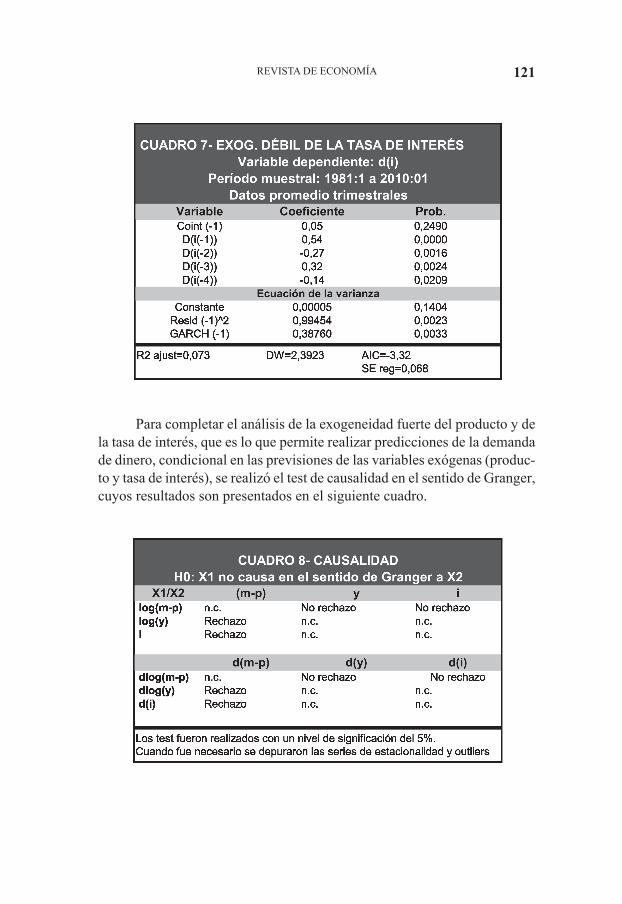
REVISTA DE ECONOMÍA 121
Para completar el análisis de la exogeneidad fuerte del producto y de la tasa de interés, que es lo que permite realizar predicciones de la demanda de dinero, condicional en las previsiones de las variables exógenas (produc-to y tasa de interés), se realizó el test de causalidad en el sentido de Granger, cuyos resultados son presentados en el siguiente cuadro.

122 CONRADO BRUM, ELIZABETH BUCACOS, PATRICIA CARBALLO
Como puede observarse la evidencia encontrada apunta a rechazar las hipótesis de que el producto y la tasa de interés no causan en el sentido de Granger a la cantidad real de dinero. Esto se cumple tanto en niveles como en diferencias de las variables.11 Asimismo, no fue posible rechazar las hipótesis de que la cantidad real de dinero no causa en el sentido de Granger al producto y a la tasa de interés.
III.4 Principales Resultados
El modelo especificado implica una serie de avances en materia de modelización de la demanda de dinero en Uruguay.
En primer lugar, la incorporación de la variable vt logró captar, al menos en parte, el proceso de desmonetización que experimentó la econo-mía uruguaya durante los años ochenta, la recuperación moderada de los noventa, y la fuerte remonetización de los últimos años. No resultó signifi-cativa la tendencia determinista que los antecedentes consultados asociaban a innovaciones tecnológicas. Es muy probable que parte del efecto de esta variable haya sido captado por la propia variable vt .
En segundo lugar, se estimó una elasticidad-ingreso de largo plazo de la demanda de dinero unitaria, en línea con lo postulado por la teoría económica.
Por otra parte, la exogeneidad fuerte del producto y la tasa de interés, que son las variables explicativas de la demanda de dinero y además forman parte del vector cointegrador, habilita a realizar predicciones de la demanda de dinero.
Los errores de predicción pueden provenir de tres fuentes distintas: errores en la estimación de los estimadores, errores en las proyecciones de las variables exógenas y errores estocásticos inherentes al propio modelo. El no rechazo de la hipótesis de estabilidad del modelo, y el hecho de que las proyecciones de las variables exógenas provengan de otros modelos externos a la demanda de dinero, permiten concentrarse en los errores de previsión inherentes al propio modelo. Para ello se tomaron como dados los valores de las variables exógenas y se mantuvieron constantes las estima-ciones de los parámetros realizadas para toda la muestra.
11 Si bien el Test de Causalidad en el sentido de Granger debe realizarse con variables esta-cionarias, el hecho de que las mismas estén cointegradas llevó a que además se realizara el contraste con las variables en nivel.

REVISTA DE ECONOMÍA 123
Siguiendo esta línea, se evaluó la capacidad predictiva del modelo a partir de los estadísticos habituales que se construyen para tal fin: la Raíz del Error Cuadrático Medio (RECM), Error Medio (EM) y Error Absoluto Medio (EAM).
En primer lugar, el comportamiento del error medio, que para todos los horizontes se ubica cercano a cero, sugiere que los errores de proyec-ción, como era de esperar, no tienen un sesgo sistemático en el período evaluado.
Por otra parte, los resultados que surgen de los estadísticos RECM y EAM sugieren que el error de predicción se reduce a medida que se aleja el horizonte de proyección. Esto era esperable por tratarse de un modelo de corrección de errores. Al considerar el horizonte de proyección de la políti-ca monetaria -6 trimestres- estos estadísticos arrojan un error promedio que se ubica entre 3% y 4%. Estos hallazgos justifican la utilización del modelo de demanda de dinero para la programación monetaria de mediano plazo.

124 CONRADO BRUM, ELIZABETH BUCACOS, PATRICIA CARBALLO
IV. CONCLUSIONES
En este documento se presentó un modelo de corrección de errores para la demanda real de dinero para el período 1981.1-2010.1. Este mode-lo, además de los fundamentos tradicionales –producto y tasa de interés-, incluye una variable que mide la volatilidad relativa de los rendimientos reales del dinero y un activo sustituto.
El modelo se estimó siguiendo el procedimiento de estimación à la Engle-Granger. En una primera etapa, se encontró una relación de largo plazo entre la cantidad real de dinero, el nivel de actividad económica y la tasa de interés, estimándose una elasticidad-ingreso unitaria y una semie-lasticidad-tasa de interés negativa, en línea con lo postulado por la teoría económica. La participación de la variable “volatilidad” en la estimación de la relación de largo plazo resultó relevante para captar, al menos en parte, el fenómeno de desmonetización de los 80’s, la relativa recuperación de los 90’s y la fuerte remonetización de los últimos seis años.
Una vez obtenidos los residuos de la relación de cointegración y contrastada la exogeneidad débil del producto y la tasa de interés, se especificó un modelo de corrección de errores para la tasa de crecimien-to de la cantidad real de dinero. Ante un desvío en la cantidad real de dinero con relación a su nivel de largo plazo, la tasa de variación de la cantidad real de dinero reacciona corrigiendo dicho desequilibrio a una velocidad relativamente alta. La demanda real de dinero estimada cum-ple con los requisitos habituales de estabilidad, obteniéndose residuos bien comportados.
Adicionalmente, se analizó la exogeneidad fuerte de las variables consideradas obteniéndose evidencia de que el producto y la tasa de interés tienden a anticipar temporalmente a la cantidad real de dinero, no existien-do retroalimentación. Esto, sumado a la exogeneidad débil, implica la exo-geneidad fuerte de las variables explicativas consideradas, lo que habilita la utilización del modelo con fines predictivos de la demanda de dinero.

REVISTA DE ECONOMÍA 125
Finalmente, se evaluó la capacidad predictiva del modelo a distintos horizontes. Los resultados encontrados sugieren que el modelo es adecuado para ser utilizado en la programación monetaria de mediano plazo.
Del modelo de demanda de dinero estimado se derivan algunos ele-mentos que permiten ser optimistas en cuanto al futuro de la política mone-taria. El fenómeno de desmonetización que atravesó la economía uruguaya durante los años ochenta, que en su momento fuera pensado como perma-nente, fue finalmente revertido, iniciándose luego un fuerte y sostenido pro-ceso de remonetización. Este fenómeno fue viabilizado por la aplicación de una política monetaria orientada a alcanzar una inflación baja y estable, y sin compromisos cambiarios. La profundización de esta política permitiría entrar en un círculo virtuoso que ayude a consolidar la desdolarización de la economía, potenciando a la propia política monetaria.

126 CONRADO BRUM, ELIZABETH BUCACOS, PATRICIA CARBALLO
V. REFERENCIAS BIBLIOgRÁFICAS
Bucacos, Elizabeth y Gerardo Licandro (2002). “La demanda de dinero en Uruguay: 1980.1 -2002.4”. Revista de Economía del BCU, noviembre de 2003.
Bucacos, Elizabeth (2005). “Acerca de la estacionalidad estocástica. Una aplicación para la demanda de dinero en Uruguay”. Revista de Economía del BCU, noviembre de 2005.
Clower, Robert W., (1967). “A reconsideration of the microfoundations of monetary theory”. Western Economic Journal, 6, 1-8.
Della Mea, Umberto (1990). “La demanda por medios de pago, revisitada”, Revista de Economía, Vol. V, Nº 2-3, Diciembre 1990-Abril 1991, Banco Central del Uruguay.
Della Mea, Umberto y Daniel Dominioni (1992). “Tendencias y predicti-bilidad de la base monetaria uruguaya: los años recientes”. Trabajo presen-tado en las séptimas Jornadas Anuales de Economía del Banco Central del Uruguay.
Fernández, S., (1999). “Un modelo para la demanda de dinero en Uruguay (1983-1998)”. Trabajo de Investigación Monográfica. Licenciatura en Eco-nomía. Facultad de Ciencias Económicas y Administración, Universidad de la República.
Fried, Alejandro y José M. Trujillo (2006). “Demanda de dinero en Uru-guay: una nueva aproximación”. Documento presentado en las Jornadas de Economía 2006 del BCU.
Gagliardi, Enrique (2007). “Macroeconomía de economías pequeñas y abiertas”. Tomo I, Segunda Edición. Universidad ORT, Central de Impre-siones Ltda.

REVISTA DE ECONOMÍA 127
Lucas Jr., Robert, (1980). “Two illustrations of the quantity of money”. American Economic Review, 70 (5), 1005-1014.
Markowitz, Harry M. (1952). “Portfolio Selection”. The Journal of Finan-ce, marzo de 1952.
Novales, Alfonso (1993). “Econometría”. Segunda Edición.
Pascale, Ricardo. “Decisiones Financieras” (2003). Ediciones de la Plaza. 4ª Edición Revisada.
Sidrauski, Miguel (1967). “Inflation and economic growth”. Journal of Po-litical Economy, 75, 534-544.
Tobin James (1958). “Liquidity preference as a behaviour toward risk”, Review of Economic Studies, Febrero de 1958.
Wilson, Charles (1989). “An infinite horizon model with money”, in Green and J.A. Scheinkman (eds.), General Equilibrium, growth and trade, New York, Academic Press.

Gráfica Industrial Uruguaya Ltda.Soriano 1128
Tel.: 2900 0108 - Fax: 2902 2576E-mail: [email protected]
ISSN: 0797-5546D.L. 356968 - Noviembre de 2011